Resumming the color-octet contribution to $e^{+}e^{-}\to J/\psi+X$

Abstract

Recent observations of the spectrum of $J/\psi$ produced in $e^{+}e^{-}$ collisions at the $\Upsilon(4S)$ resonance are in conflict with fixed-order calculations using the Non-Relativistic QCD (NRQCD) effective field theory. One problem is that leading order color-octet mechanisms predict an enhancement of the cross section for $J/\psi$ with maximal energy that is not observed in the data. However, in this region of phase space large perturbative corrections (Sudakov logarithms) as well as enhanced nonperturbative effects are important. In this paper we use the newly developed Soft-Collinear Effective Theory (SCET) to systematically include these effects. We find that these corrections significantly broaden the color-octet contribution to the $J/\psi$ spectrum. Our calculation employs a one-stage renormalization group evolution rather than the two-stage evolution used in previous SCET calculations. We give a simple argument for why the two methods yield identical results to lowest order in the SCET power counting.

I Introduction

Bound states of heavy quarks and antiquarks have been of great interest since the discovery of the $J/\psi$ psi . In particular the production of quarkonium is an interesting probe of both perturbative and nonperturbative aspects of QCD dynamics. Production requires the creation of a heavy $Q\bar{Q}$ pair with energy greater than $2m_{Q}$, a scale at which the strong coupling constant is small enough that perturbation theory can be used. However, hadronization probes much smaller mass scales of order $m_{Q}v^{2}$, where $v$ is the typical velocity of the quarks in the quarkonium. For $J/\psi$, $m_{Q}v^{2}$ is numerically of order $\Lambda_{\rm QCD}$ so the production process is sensitive to nonperturbative physics as well.

A systematic theoretical framework for handling the different scales characterizing both the decay and production of quarkonium is Non-Relativistic Quantum Chromodynamics (NRQCD) Bodwin:1995jh ; Luke:2000kz . NRQCD solves important conceptual as well as phenomenological problems in quarkonium theory. For instance, perturbative calculations of the inclusive decay rates for $\chi_{c}$ mesons in the color-singlet model suffer from nonfactorizable infrared divergences Barbieri:1976fp . NRQCD provides a generalized factorization theorem that includes nonperturbative corrections to the color-singlet model, including color-octet decay mechanisms. All infrared divergences can be factored into nonperturbative matrix elements, so that infrared safe calculations of inclusive decay rates are possible Bodwin:1992ye . In addition, color-octet production mechanisms are critical for understanding the production of $J/\psi$ at large transverse momentum, $p_{\perp}$, at the Fermilab Tevatron tevatron . NRQCD has been applied to the production and decay of quarkonium in various experimental settings. However, there are still many challenging problems in quarkonium physics that remain to be solved Bodwin:2002mr . One important problem is the polarization of $J/\psi$ at the Tevatron. NRQCD predicts the $J/\psi$ should become transversely polarized as the $p_{\perp}$ of the $J/\psi$ becomes much larger than $2m_{c}$ psipol . The theoretical prediction is consistent with the experimental data at intermediate $p_{\perp}$, but at the largest measured values of $p_{\perp}$ the $J/\psi$ is observed to be slightly longitudinally polarized. At these $p_{\perp}$, discrepancies at the 3$\sigma$ level are seen in both prompt $J/\psi$ and $\psi^{\prime}$ polarization measurements poldata .

New problems have arisen as a result of recent measurements of the spectra of $J/\psi$ produced at the $\Upsilon(4S)$ resonance in $e^{+}e^{-}$ collisions by the BaBar and Belle experiments Abe:2001za ; Aubert:2001pd . Leading order NRQCD calculations predict that for most of the range of allowed energies prompt $J/\psi$ production should be dominated by color-singlet production mechanisms, while color-octet contributions dominate when the $J/\psi$ energy is nearly maximal. Furthermore, as pointed out in Ref. Braaten:1995ez , color-octet processes predict a dramatically different angular distribution for the $J/\psi$. Writing the differential cross section as

$$\frac{d\sigma}{dp_{\psi}\,d\cos\theta}=S(p_{\psi})(1+A(p_{\psi})\cos^{2}\theta)\,,$$ (1)

where $p_{\psi}$ is the $J/\psi$ momentum and $\cos\theta$ is the angle of the $J/\psi$ with respect to the axis defined by the $e^{+}e^{-}$ beams, one finds the color-singlet mechanism gives $A(p_{\psi})\approx 0$ except for large $p_{\psi}$, where $A(p_{\psi})$ becomes large and negative. On the other hand, color-octet production predicts $A(p_{\psi})\approx 1$. The significant enhancement of the cross section accompanied by the change in angular distribution were proposed as a distinctive signal of color-octet mechanisms in Ref. Braaten:1995ez . It was expected that these effects would be confined to $J/\psi$ whose momentum is within a few hundred MeV of the maximum allowed.

Experimental results do not agree with these expectations. The cross section data as a function of momentum is binned in intervals of 300 or 500 MeV, depending on the experiment, and the data does not exhibit any enhancement in the bins closest to the endpoint. However, the total cross section measured by the two experiments exceeds predictions based on the color-singlet model alone. The total prompt $J/\psi$ cross section, which includes feeddown from $\psi^{\prime}$ and $\chi_{c}$ states but not from $B$ decays, is measured to be $\sigma_{tot}=2.52\pm 0.21\pm 0.21$ pb by BaBar, while Belle measures $\sigma_{tot}=1.47\pm 0.10\pm 0.13$ pb. Estimates of the color-singlet contribution range from $0.4-0.9$ pb Cho:1996cg ; Yuan:1996ep ; Baek:1998yf ; Schuler:1998az . Furthermore, $A(p_{\psi})$ is measured to be consistent with $1$ (with large errors) for $p_{\psi}>2.6\,{\rm GeV}$ (Belle) and $p_{\psi}>3.5\,{\rm GeV}$ (BaBar). These aspects of the data suggest that there is a substantial color-octet contribution which is not confined to the very endpoint of the momentum spectrum but spread over a substantially broader range of momentum.

In this paper, we will argue that higher order perturbative and nonperturbative corrections that are enhanced near the endpoint give rise to a broad color-octet contribution. The calculation depends on a nonperturbative function, called a shape function, which parametrizes the distribution of lightcone momentum of the $J/\psi$ carried by the color-octet $c\bar{c}$ pair produced in the short-distance process. Since the shape function is nonperturbative, our calculation is not predictive. However, moments of the shape function are NRQCD operators whose size is constrained by the velocity scaling rules of NRQCD. Choosing a simple ansatz for the shape function whose moments are consistent with velocity scaling rules, we find that the combined perturbative and nonperturbative effects lead to substantial broadening of the color-octet spectrum in a manner that is consistent with data. Since the shape function that appears in this calculation also appears in other processes, it could be extracted from $e^{+}e^{-}$ data and used to make predictions for photoproduction and electroproduction once resummed calculations for these processes become available. Ref. Beneke:1999gq presents a calculation of $J/\psi$ photoproduction which includes a nonperturbative shape function but not the resummation of large perturbative corrections. An important point of this paper is that nonperturbative and perturbative corrections combine to produce a spectrum that is broader than that obtained when only one of the corrections is included. Therefore it would be interesting to revisit the calculation of photoproduction using the methods of this paper.

While the calculations of this paper show that the leading color-octet contribution is broad enough to be compatible with the observed $p_{\psi}$ distributions, other features of the $e^{+}e^{-}$ data remain puzzling. In particular, Belle reports a large cross section for $J/\psi$ produced along with open charm Abe:2002rb :

$$\frac{\sigma(e^{+}e^{-}\rightarrow J/\psi c\bar{c})}{\sigma(e^{+}e^{-}\rightarrow J/\psi X)}=0.59^{+0.15}_{-0.13}\pm 0.12\,.$$

The predicted ratio from leading order color-singlet production mechanisms alone is about $0.2$ Cho:1996cg ; Baek:1998yf and a large color-octet contribution makes this ratio even smaller. In addition to the inclusive measurements, Belle reports a cross section for exclusive double charmonium production which exceeds previous theoretical estimates. Recent attempts to address the latter problem can be found in Ref. double .

The experiments also measure the polarization of the $J/\psi$, which can provide important information about the production mechanism. Unfortunately the current experimental situation is unclear. Polarization is studied by measuring

$$\alpha=\frac{1-3\eta_{L}}{1+\eta_{L}}\,,$$

where $\eta_{L}$ is the fraction of $J/\psi$ which are longitudinally polarized. Both BaBar and Belle measure $\alpha\approx-0.5$ for $p_{\psi}<3.5$ GeV. However, for $p_{\psi}>3.5$ GeV BaBar measures $\alpha=-0.8\pm 0.09$, corresponding to almost completely longitudinally polarized $J/\psi$, while Belle measures $\alpha=-0.2\pm 0.2$, which is consistent with no polarization. Neither measurement attempts to correct for feeddown effects on the polarization of the $J/\psi$. Measurements of the polarization of directly produced $J/\psi$ can discriminate between various production mechanisms Baek:1998yf . The color-singlet process $e^{+}e^{-}\rightarrow J/\psi\overline{c}c$ produces $J/\psi$ with $\alpha$ rising from zero at $p_{\psi}=0$ to 1 at the kinematic endpoint for this process. The color-singlet process $e^{+}e^{-}\rightarrow J/\psi gg$ prefers longitudinally polarized $J/\psi$ with $\alpha$ decreasing to almost $-1$ at the kinematic endpoint. Finally, the leading order color-octet diagrams produce $J/\psi$ with $\alpha$ between 0 and -0.07, depending on the relative importance of $S$-wave and $P$-wave production mechanisms.

The NRQCD factorization formalism shows that the differential $J/\psi$ cross section can be written as

$$d\sigma(e^{+}e^{-}\rightarrow J/\psi+X)=\sum_{n}d\hat{\sigma}(e^{+}e^{-}\rightarrow c\bar{c}[n]+X)\langle{\cal O}^{J/\psi}_{n}\rangle\,,$$ (2)

where $d\hat{\sigma}$ is the inclusive cross section for producing a $c\bar{c}$ pair in a color and angular momentum state labeled by $[n]={}^{2S+1}L_{J}^{(i)}$. In this notation, the spectroscopic notation for angular momentum quantum numbers is standard and $i=1(8)$ for color-singlet(-octet) production matrix elements. The short-distance coefficients are calculable in a perturbation series in $\alpha_{s}$. The long-distance matrix elements $\langle{\cal O}^{J/\psi}_{n}\rangle$ are vacuum matrix elements of four-fermion operators in NRQCD Bodwin:1995jh . These matrix elements scale as some power of the relative velocity $v\ll 1$ of the $c$ and $\bar{c}$ quarks as given by the NRQCD power-counting rules.

At lowest order in $v$ the only term in Eq. (2) is the color-singlet contribution, $[n]={}^{3}S_{1}^{(1)}$, which scales as $v^{3}$. The coefficient for this contribution starts at $O(\alpha^{2}_{s})$ csrate . Away from the kinematic endpoint $E_{max}=(s+M_{\psi}^{2})/(2\sqrt{s})$, where $s$ is the center-of-mass energy squared, color-octet contributions also start at $O(\alpha_{s}^{2})$. Since the color-octet contributions are suppressed by $v^{4}\approx 0.1$ relative to the leading color-singlet contribution, they are negligible throughout most of the allowed phase-space at leading order in perturbation theory. However, as pointed out in Ref. Braaten:1995ez , there is an $O(\alpha_{s})$ contribution to color-octet production from the diagrams shown in Fig. 1.

Figure 1: Leading order short distance amplitudes for $e^{+}e^{-}\to c\bar{c}+g$ in QCD.

In this process the $c\bar{c}$ are in either a ${}^{1}S_{0}^{(8)}$ or ${}^{3}P_{J}^{(8)}$ configuration. The resulting cross sections are proportional to a $\delta-$function which forces the energy of the $c\bar{c}$ pair to be maximal Braaten:1995ez :

$$\frac{d\hat{\sigma}[^{1}S_{0}^{(8)}]}{dz\,d\cos{\theta}} = \delta(1-z)\frac{4\pi^{2}\alpha^{2}\alpha_{s}e^{2}_{c}}{s^{2}m_{c}}(1-r)(1+\cos^{2}{\theta}),$$ (3)

$$\frac{d\hat{\sigma}[{}^{3}P_{0}^{(8)}]}{dz\,d\cos{\theta}} = \delta(1-z)\frac{8\pi^{2}\alpha^{2}\alpha_{s}e^{2}_{c}}{s^{2}m_{c}^{3}}\frac{(3+6r+7r^{2})+(3-10r+7r^{2})\cos^{2}{\theta}}{2(1-r)}\,,$$

where $r=4m^{2}_{c}/s$, and $z=E_{c\bar{c}}/E^{max}_{c\bar{c}}$ with $E^{max}_{c\bar{c}}=\sqrt{s}(1+r)/2$. Here we have used $\langle{\cal O}^{\psi}_{8}(^{3}P_{J})\rangle=(2J+1)\langle{\cal O}^{\psi}_{8}(^{3}P_{0})\rangle$ and combined the short-distance cross sections for the three $P$-wave contributions. For comparison, in this region of phase space the color-singlet contribution approaches a constant

$$\lim_{z\rightarrow 1}\frac{d\hat{\sigma}[{}^{3}S_{1}^{(1)}]}{dz\,d\cos{\theta}}=\frac{64\pi\alpha^{2}\alpha^{2}_{s}e^{2}_{c}}{27s^{2}m_{c}}(1+r)\Bigg{(}\frac{1+r}{1-r}-\cos^{2}{\theta}\Bigg{)}\,.$$ (4)

We see that the $v^{4}$ suppression of the color-octet contribution is compensated by one power of $\alpha_{s}$. In addition, the numerical coefficient of the color-octet contributions is bigger by a factor of $\approx 4\pi$ which is due to the difference between two- and three-body phase space. Since the color-octet contribution is proportional to a singular distribution, sensible comparison with data requires that we integrate the cross section over a region in $z$ of finite size. It is important to know what range of $z$ must be integrated over in order for the leading order calculation to be reliable. Ref. Beneke:1997qw has identified a class of nonperturbative corrections which are suppressed by powers of $v^{2}$ but are enhanced by factors of $1/(1-z)$, so we must integrate from a lower limit no larger than $z_{min}\sim 1-v^{2}$. For $z_{min}\sim 1-v^{2}$ , the integrated color-singlet cross section gets an additional $v^{2}$ suppression relative to the color-octet contribution so the ratio of the integrated color-octet to integrated color-singlet is $\sim 4\pi v^{2}/\alpha_{s}$ which is roughly a factor of 10.

Note that because $v^{2}\approx 0.3$ for $J/\psi$, the cross section must be integrated over a substantial region. For production at the $\Upsilon(4S)$, $E_{max}=5.74$ GeV, corresponding to $p_{max}=4.84$ GeV, so we must integrate above $E\approx 4.0$ GeV, which corresponds to $p_{\psi}\approx 2.5$ GeV. These numbers show that the spectrum reported in Refs. Abe:2001za ; Aubert:2001pd , which plot the data as a function of $p_{\psi}$, cannot be directly compared to the leading order NRQCD calculation. Nonperturbative effects smear the color-octet contribution over nearly half the range of allowed momenta, so the color-octet contribution is not confined to the last momentum bin. Higher order perturbative corrections are also important. The next-to-leading order radiative correction to color-octet production has a contribution proportional to $\alpha_{s}\log(1-z)/(1-z)$, so perturbative corrections require a resummation when $1-z\sim\alpha_{s}$. Since $\alpha_{s}\sim v^{2}$, similar conclusions regarding the reliability of the leading order calculation arise from purely perturbative considerations.

Large perturbative and nonperturbative corrections signal that the NRQCD factorization theorem of Eq. (2) is no longer valid. The problem is that near the endpoint the $J/\psi$ is recoiling against a gluon jet with energy of order $M_{\Upsilon}$ but mass of order $M_{\Upsilon}\sqrt{\Lambda_{\rm QCD}/M_{\psi}}$. These degrees of freedom are integrated out of NRQCD, but when we probe the endpoint region they must be kept as explicit degrees of freedom. The effective theory which correctly describes this kinematic regime is a combination of NRQCD for the heavy degrees of freedom, and the Soft-Collinear Effective Theory (SCET) Bauer:2001ew ; Bauer:2001yr ; Bauer:2001ct ; Bauer:2001yt for the light energetic degrees of freedom. The factorization theorem derived using NRQCD and SCET will include a nonperturbative distribution that incorporates the $v^{2n}/(1-z)^{n}$ nonperturbative corrections to all orders. In addition, renormalization group equations of SCET can be used to resum large perturbative corrections. A similar treatment of nonperturbative and perturbative endpoint corrections to the color-octet contributions in the inclusive decay $\Upsilon\rightarrow X+\gamma$ can be found in Ref. Bauer:2001rh .

II Factorization

In this section, we present the factorization theorem for $J/\psi$ production near the kinematic endpoint. We begin by studying the kinematics of the process to determine when NRQCD breaks down and SCET must be used instead. In the $e^{+}e^{-}$ center-of-mass (COM) frame, the $c\bar{c}$ pair has momentum $p_{c\bar{c}}^{\mu}=Mv^{\mu}+\ell^{\mu}$, where $M=2m_{c}$, $\ell^{\mu}$ is the residual momentum of the $c\bar{c}$ pair and the four-velocity of the $J/\psi$ is

$$v^{\mu}=\frac{1}{2}\Bigg{(}\frac{M_{\psi}}{x\sqrt{s}}n^{\mu}+\frac{x\sqrt{s}}{M_{\psi}}{\bar{n}}^{\mu}\Bigg{)}\,.$$ (5)

Here $M_{\psi}$ is the $J/\psi$ mass and $x=(E_{\psi}+p_{\psi})/\sqrt{s}$. The residual momentum arises because the $c\bar{c}$ pair is produced along with ultrasoft (usoft) quanta which carry $O(\Lambda_{\rm QCD})$ momentum in the rest frame of the $J/\psi$. The lightlike vectors are ${\bar{n}}^{\mu}=(1,0,0,1)$ and $n^{\mu}=(1,0,0,-1)$, where the $J/\psi$ is moving in the $z$ direction in the COM frame. It is sometimes helpful to write $\ell^{\mu}$ in terms of the boost that takes one from the $J/\psi$ rest frame to the COM frame: $\ell^{\mu}=\Lambda^{\mu}{}_{\nu}\hat{\ell}^{\nu}$. The components of $\hat{\ell}^{\mu}$ are ${O}(\Lambda_{\rm QCD})$ while the components of $\ell^{\mu}$ scale as: $\bar{n}\cdot\ell\sim M_{\psi}\Lambda_{\rm QCD}/(x\sqrt{s}),n\cdot\ell\sim x\sqrt{s}\Lambda_{\rm QCD}/M_{\psi}$ and $\ell_{\perp}\sim\Lambda_{\rm QCD}$. The momentum of the virtual photon is $q^{\mu}=\sqrt{s}/2(n^{\mu}+{\bar{n}}^{\mu})$ and the gluon jet has momentum

$$p^{\mu}_{X}=\frac{\sqrt{s}}{2}\Bigg{[}\Bigg{(}1-\frac{r}{\hat{x}}\Bigg{)}n^{\mu}+(1-\hat{x})\bar{n}^{\mu}\Bigg{]}-\ell^{\mu}\,,$$ (6)

where $\hat{x}=xM/M_{\psi}$. Away from the endpoint region ($x\ll 1$) the recoiling gluon jet momentum and invariant mass are both of order $\sqrt{s}$. Therefore, the jet can be integrated out of the theory and one obtains the NRQCD factorization formula in Eq. (2). In this region $\ell^{\mu}$ is negligible compared to the large components of $p_{X}^{\mu}$ and $p_{c\bar{c}}^{\mu}$ and can be set to zero. Therefore the cross section is not sensitive to motion of the $c\bar{c}$ within the $J/\psi$. This is evident from the NRQCD factorization formula which depends on a single nonperturbative parameter, $\langle{\cal O}(^{1}S_{0}^{(8)})\rangle$ or $\langle{\cal O}(^{3}P_{0}^{(8)})\rangle$. When $1-x\sim\Lambda_{\rm QCD}/M\sim v^{2}$, $\sqrt{s}(1-x)$ is the same size as $n\cdot\ell$, so the residual momentum cannot be neglected. In the endpoint region, the NRQCD factorization formula breaks down. A new factorization theorem is needed which includes a distribution function that parametrizes the nonperturbative motion of the $c\bar{c}$ pair within the jet containing the $J/\psi$. For $1-x=1/3$, $p_{\psi}=2.8$ GeV, so the new factorization theorem is relevant for a significant part of the measured $p_{\psi}$ spectrum. The failure of NRQCD factorization can also be understood by considering the gluon jet which was integrated out. When $1-x\sim\Lambda_{\rm QCD}/M$ the jet is no longer highly virtual:

$$m_{X}^{2}\sim\Lambda_{\rm QCD}s/M\,.$$ (7)

Since $m_{X}^{2}/E_{X}^{2}\sim\Lambda_{\rm QCD}/M\ll 1$, the gluon jet is composed of energetic particles with small invariant mass that must be included explicitly in the effective theory.

SCET has collinear degrees of freedom whose momentum scales as $\bar{n}\cdot p\sim Q$, $n\cdot p\sim\lambda^{2}Q$, and $p^{\perp}\sim\lambda Q$. For the process under consideration, $Q$ is of order $\sqrt{s}$, while $\lambda\sim\sqrt{1-x}\sim(\Lambda_{\rm QCD}/M)^{1/2}$. SCET also has soft degrees of freedom whose momentum scales as $\lambda$ and usoft degrees of freedom whose momentum scales as $\lambda^{2}$. Heavy quark fields in SCET are the same as in NRQCD when considering quarkonium. Since a field redefinition removes the large $O(m_{c},m_{c}v)$ part of their momentum, derivatives on these fields scale as $\Lambda_{\rm QCD}$ and therefore they are usoft fields in SCET. Thus the endpoint region of $J/\psi$ production is mediated by SCET operators involving usoft (heavy) quark fields and collinear gluon fields. Soft fields do not enter to the order we are working, so are neglected.

To match onto SCET, matrix elements in QCD are evaluated at the scale $Q$ and expanded in powers of $\lambda$. Each order in the $\lambda$ expansion is reproduced in the effective theory by a product of Wilson coefficients (which depend only on the large scale $Q$) and SCET operators. At each order, one must include all SCET operators which can contribute to the process under consideration, subject to the restriction that the operators respect the symmetries of the effective theory. In SCET, gauge transformations can be classified by their scaling with $\lambda$ just like fields Bauer:2001yt . For $e^{+}e^{-}\rightarrow J/\psi+X$, the relevant operators must be invariant under collinear and usoft gauge transformations Bauer:2001yt . SCET is not Lorentz invariant, but the Lorentz invariance of QCD is realized in the form of constraints on the possible operators which appear in the Lagrangian and in matching calculations. These constraints are called reparametrization invariance (RPI) Manohar:2002fd . Usoft and collinear gauge invariance and RPI uniquely fix the form of the lowest order operators contributing to $e^{+}e^{-}\rightarrow J/\psi+X$.

In the collinear sector of SCET there is a collinear fermion field $\xi_{n,p}$, a collinear gluon field $A_{n,q}^{\mu}$, and a collinear Wilson line

$$W_{n}(x)=\bigg{[}\sum_{\rm perms}{\rm exp}\left(-g_{s}\frac{1}{\bar{\cal P}}{\bar{n}}\cdot A_{n,q}(x)\right)\bigg{]}\,.$$ (8)

The subscripts on the collinear fields are the lightcone direction $n^{\mu}$, and the large components of the lightcone momentum (${\bar{n}}\cdot q,q_{\perp}$). The operator ${\cal P}^{\mu}$ projects out the momentum label Bauer:2001ct . For example ${\bar{n}}\cdot{\cal P}\xi_{n,p}\equiv\bar{\cal P}\xi_{n,p}={\bar{n}}\cdot p\,\xi_{n,p}$. Likewise in the usoft sector there is a usoft fermion field $q_{us}$, a usoft gluon field $A^{\mu}_{us}$, and a usoft Wilson line $Y$. Using the transformations for each of these fields under collinear and usoft gauge transformations given in Ref. Bauer:2001yt , we can build invariant operators. The collinear-gauge invariant field strength is

$$G^{\mu\nu}_{n}\equiv-\frac{i}{g_{s}}W^{\dagger}[i{\cal D}_{n}^{\mu}+g_{s}A_{n,q}^{\mu},i{\cal D}_{n}^{\nu}+g_{s}A_{n,q^{\prime}}^{\nu}]W,$$ (9)

where

$$i{\cal D}_{n}^{\mu}=\frac{n^{\mu}}{2}\bar{\cal P}+{\cal P}_{\perp}^{\mu}+\frac{{\bar{n}}^{\mu}}{2}in\cdot D,$$ (10)

and $iD^{\mu}=i\partial^{\mu}+g_{s}A^{\mu}_{us}$ is the usoft covariant derivative. RPI invariance requires the label operators and the usoft covariant derivatives, which scale differently with $\lambda$, to appear in the linear combination appearing in $i{\cal D}_{n}^{\mu}$. The leading piece of $G^{\nu\mu}_{n}$ is order $\lambda$ and can be written as ${\bar{n}}_{\nu}G^{\nu\mu}_{n}=i[\bar{\cal P},B^{\mu}_{\perp}]$, where

$$B^{\mu}_{\perp}=\frac{1}{g_{s}}W^{\dagger}({\cal P}_{\perp}^{\mu}+g_{s}(A^{\mu}_{n,q})_{\perp})W.$$ (11)

The subscript $\perp$ on $B_{\perp}^{\mu}$ indicates that $\mu$ must be a perpendicular direction. The leading operator for $e^{+}e^{-}\rightarrow c\bar{c}g$ must have a $(A^{\mu}_{n,q})_{\perp}$ field operator to create the collinear gluon in the final state. $B^{\mu}_{\perp}$ is the collinear gauge invariant generalization of this field.

The $O(\lambda)$ operator which creates a heavy quark and antiquark in a ${}^{1}S_{0}$ state with a collinear gluon is

$$\psi^{\dagger}_{{\bf p}}\,\Gamma^{(8,{}^{1}S_{0})}_{\alpha\mu}(-n\cdot v\,\bar{\cal P};\mu)B^{\alpha}_{\perp}\chi_{-\bf p}\,.$$ (12)

This is collinear gauge invariant because $B_{\perp}^{\mu}$ is invariant and the heavy quark fields do not transform under collinear gauge transformation. It is also usoft gauge invariant since

$$\chi_{-{\bf p}}\rightarrow V_{\rm us}\chi_{-{\bf p}},\qquad\psi_{\bf p}\rightarrow V_{\rm us}\psi_{\bf p},\qquad B^{\alpha}_{\perp}\rightarrow V_{\rm us}B^{\alpha}_{\perp}V^{\dagger}_{\rm us}\,,$$ (13)

under usoft gauge transformations. Type-III reparametrization invariance Manohar:2002fd requires $\bar{\cal P}$ to appear multiplied by $n\cdot v$ Pirjol:2002km . The operator is not invariant under type-I and -II transformations but can be made invariant by adding $\lambda$ suppressed operators which are not needed at the order we are working. The factor of $-\bar{\cal P}$ in Eq. (12) gives the large component of the momentum of the jet at the endpoint. This is the part of ${\bar{n}}\cdot p_{X}$ that survives as $\Lambda_{\rm QCD}/M$ and $1-x\rightarrow 0$, so that $-n\cdot v\,\bar{\cal P}=s(1-r)/M$. At leading order, the function $\Gamma^{(8,{}^{1}S_{0})}_{\alpha\mu}$ is determined by requiring the SCET matrix element of Eq. (12) to agree with the lowest order QCD diagrams for $e^{+}e^{-}\rightarrow c\bar{c}g$, shown in Fig. 2:

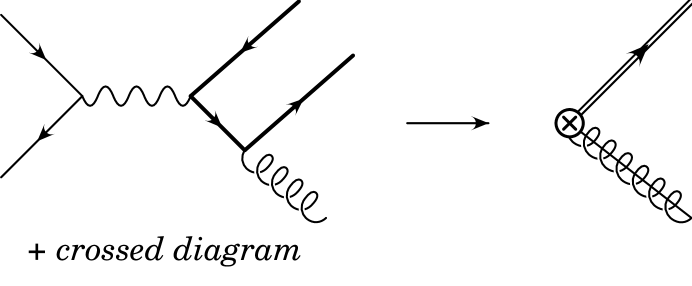
Figure 2: Matching the production amplitude for $e^{+}e^{-}\to c\bar{c}+g$ in QCD and SCET. Collinear gluons are represented by a spring with a line through it.

$$\Gamma^{(8,{}^{1}S_{0})}_{\alpha\mu}=\frac{2g_{s}ee_{c}}{M}\epsilon_{\alpha\mu}^{\perp}\,,$$ (14)

where $\epsilon_{\alpha\mu}^{\perp}=\epsilon^{\perp}_{\alpha\mu\rho\beta}{\bar{n}}^{\rho}n^{\beta}/2$. The leading SCET color-octet ${}^{3}P_{J}$ operator is

$$\psi^{\dagger}_{{\bf p}}\Gamma^{(8,{}^{3}P_{J})}_{\alpha\mu\sigma\delta}(-n\cdot v\bar{\cal P};\mu)B^{\alpha}_{\perp}\Lambda\cdot\widehat{{\bf p}}^{\sigma}\Lambda\cdot\mbox{\boldmath$\sigma$}^{\delta}\chi_{-\bf p}\,,$$ (15)

where $\widehat{{\bf p}}={\bf p}/M$ and the leading order matching coefficient is

$$\Gamma^{(8,{}^{3}P_{J})}_{\alpha\mu\sigma\delta} = \frac{2ig_{s}ee_{c}}{M}\bigg{\{}g^{\perp}_{\alpha\sigma}\bigg{[}2\bigg{(}\frac{1+r}{1-r}\bigg{)}g_{\mu\delta}-\frac{1}{r}(1-r){\bar{n}}_{\delta}n_{\mu}\bigg{]}$$ (16)

$$\phantom{4g_{s}ee_{b}\bigg{\{}}-g^{\perp}_{\alpha\delta}\bigg{[}2g_{\mu\sigma}-\frac{1}{r}(1+r)n_{\mu}{\bar{n}}_{\sigma}\bigg{]}-g^{\perp}_{\alpha\mu}(n_{\delta}{\bar{n}}_{\sigma}+{\bar{n}}_{\delta}n_{\sigma})\bigg{\}},$$

where $g^{\perp}_{\mu\nu}=g_{\mu\nu}-(n_{\mu}{\bar{n}}_{\nu}+n_{\nu}{\bar{n}}_{\mu})/2$.

It is possible to show that the rate $e^{+}e^{-}\to J/\psi+X$ in the endpoint region can be factored into a hard coefficient $\sigma_{0}$, a collinear jet function $J$, and a usoft function $S$, as

$$\frac{d\sigma^{[n]}}{dz}=P[r,z]\sigma_{0}^{[n]}\int_{z}^{1}d\xi\,S^{[n]}(\xi)\,J(s(1+r)(\xi-z)),$$ (17)

where $z=E_{\psi}/E^{max}_{\psi}$, and

$$P[r,z]=\frac{\sqrt{(1+r)^{2}z^{2}-4r}}{1-r}$$ (18)

is a phase space factor. Note that $P[r,1]=1$. The derivation is given in Appendix A. For convenience we have integrated over $\theta$. The $\theta$ dependence of the resummed cross sections are the same as in Eq. (3).

The jet function in Eq. (17) is independent of the state of the $c\bar{c}$ pair in the $J/\psi$, and is defined as

$$J(\bar{n}\cdot p\,n\cdot k+p_{\perp}^{2}) =$$

$$-\frac{s(1+r)}{4\pi}\,{\rm Im}\left[i\int d^{4}y\,e^{ik\cdot y}\,\langle 0|T\left({\rm Tr}\left[T^{B}B^{(0)\beta}_{\perp}(y)\right]{\rm Tr}\left[T^{B}B^{(0)}_{\perp\,\beta}(0)\right]\right)|0\rangle\right],$$

where the factor $s(1+r)$ is chosen to provide a convenient normalization for the process we are interested in. $J({\bar{n}}\cdot p\,n\cdot k+p_{\perp}^{2})$ is a function of the label momenta ${\bar{n}}\cdot p$ and $p_{\perp}^{2}$, and the usoft momentum $n\cdot k$, which follows from the collinear Lagrangian containing only the $n\cdot\partial$ derivative Bauer:2001yt . Furthermore RPI requires that the jet function depends on the combination $\bar{n}\cdot p\,n\cdot k+p_{\perp}^{2}$. Here we parameterize the jet momentum so that $\bar{n}\cdot p=-\bar{n}\cdot p_{X}$ and $p_{\perp}=0$. The jet function is perturbatively calculable since it is determined by physics at the scale $\sqrt{s\Lambda_{\rm QCD}/m_{c}}\gg\Lambda_{\rm QCD}$. The $O(\alpha_{s})$ calculation of the jet function, as well as the derivation of the leading order renormalization group equations, is given in Appendix B.

The shape functions, defined in terms of usoft fields, depend on the state of the $c\bar{c}$ pair, so there are different shape functions for the ${}^{1}S_{0}^{(8)}$ and ${}^{3}P_{J}^{(8)}$ contributions. They are

$$S^{(8,^{1}S_{0})}(\ell^{+}) = \frac{\langle 0|\chi^{\dagger}_{-{\bf p}}T^{B}\psi_{\bf p}\,a_{\psi}^{\dagger}a_{\psi}\,\delta(\ell^{+}-in\cdot D)\psi^{\dagger}_{\bf p}T^{B}\chi_{-{\bf p}}|0\rangle}{4m_{c}\langle{\cal O}^{\psi}_{8}(^{1}S_{0})\rangle},$$ (20)

$$S^{(8,^{3}P_{0})}(\ell^{+}) = \frac{\langle 0|\chi^{\dagger}_{-{\bf p}}\left(-\frac{i}{2}D\cdot\sigma T^{B}\right)\psi_{\bf p}\,a_{\psi}^{\dagger}a_{\psi}\,\delta(\ell^{+}-in\cdot D)\psi^{\dagger}_{\bf p}\left(-\frac{i}{2}D\cdot\sigma T^{B}\right)\chi_{-{\bf p}}|0\rangle}{4m_{c}\langle{\cal O}^{\psi}_{8}(^{3}P_{0})\rangle},$$ (21)

where $\ell^{+}=n\cdot\ell$. Note that the combination $d\ell^{+}S^{[n]}(\ell^{+})$ is boost invariant, so $d\ell^{+}S^{[n]}(\ell^{+})=d\hat{\ell}^{+}S^{[n]}(\hat{\ell}^{+})$, where $\hat{\ell}^{+}$ is the residual momentum in the $J/\psi$ rest frame. It is useful to go to the $J/\psi$ rest frame when evaluating the shape functions, since in that frame derivatives acting on the heavy quark fields scale as $m_{c}v^{2}$. The normalizations of these functions are defined so that $\int d\ell^{+}S^{(8,^{2S+1}L_{J})}(\ell^{+})=1$. The jet function normalization is chosen so that the hard coefficients correspond to the lowest order total cross section for the color-octet contributions:

$$\sigma_{0}^{(8,^{1}S_{0})} = \frac{32\pi^{2}\alpha_{s}\alpha^{2}e_{c}^{2}}{3s^{2}}\frac{\langle{\cal O}^{\psi}_{8}(^{1}S_{0})\rangle}{m_{c}}(1-r),$$ (22)

$$\sigma_{0}^{(8,^{3}P_{0})} = \frac{32\pi^{2}\alpha_{s}\alpha^{2}e_{c}^{2}}{3s^{2}}\frac{\langle{\cal O}^{\psi}_{8}(^{3}P_{0})\rangle}{m_{c}^{3}}\frac{3+2r+7r^{2}}{1-r}.$$ (23)

To see how the factorization theorem in Eq. (17) reduces to the leading order cross section in the appropriate limit, we use the result in Appendix B for the lowest order jet function,

$$J({\bar{n}}\cdot p\,n\cdot k+p_{\perp}^{2})=\delta(\xi-z)\,,$$ (24)

where $\xi$ is defined by

$$p_{X}^{2} = s(1+r)\left[1-z+\frac{1-r}{1+r}\left(\frac{\bar{\Lambda}}{M}-\frac{\hat{\ell}^{+}}{M}\right)\right]$$ (25)

$$\equiv s(1+r)(\xi-z),$$

and $\bar{\Lambda}=M_{\psi}-M$. Then we combine Eqs. (17), (20) and (24), where $S^{[n]}$ as a function of $\xi$ is defined as

$$S^{[n]}(\xi)\equiv M\frac{1+r}{1-r}S^{[n]}(\hat{\ell}^{+}),$$ (26)

so that $\int d\xi S^{[n]}(\xi)=1$, to obtain

$$\frac{d\sigma^{(8,^{1}S_{0})}}{dz}=\frac{P[r,z]\sigma_{0}^{(8,^{1}S_{0})}}{4m_{c}\langle{\cal O}^{\psi}_{8}(^{1}S_{0})\rangle}\langle 0|\chi^{\dagger}_{-{\bf p}}T^{B}\psi_{\bf p}\,a_{\psi}^{\dagger}a_{\psi}\,\delta\left[1-z-\left(\frac{1-r}{1+r}\right)\frac{in\cdot\hat{D}-\bar{\Lambda}}{M}\right]\psi^{\dagger}_{\bf p}T^{B}\chi_{-{\bf p}}|0\rangle$$ (27)

for the ${}^{1}S_{0}^{(8)}$ contribution, for example. Here, $n\cdot\hat{D}=M_{\psi}/(x\sqrt{s})\,n\cdot D$ and scales like $m_{c}v^{2}$ or $\Lambda_{\rm QCD}$. When $1-z\gg(in\cdot\hat{D}-\bar{\Lambda})/M$, we can drop the derivatives inside the $\delta$-function and pull the $\delta$-function outside the matrix element. The final result is $d\sigma^{(8,^{2S+1}L_{J})}/dz=\sigma_{0}^{(8,^{2S+1}L_{J})}\delta(1-z)$, which agrees with Eq. (3).

III Resumming Sudakov Logarithms

The leading order color-octet contribution is proportional to $\delta(1-z)$. The next-to-leading order radiative corrections have contributions of the form $\alpha_{s}\ln(1-z)/(1-z)$. Clearly when $z\sim 1-\alpha_{s}$ these corrections are large and must be resummed. This can be accomplished in a straightforward manner by using the renormalization group equations of SCET. The resummation is most easily carried out by taking moments with respect to $z$, then the large corrections as $z\rightarrow 1$ become large logs of $N$ in the expression for the $N$th moment. In this section, the resummation for the color-octet ${}^{1}S_{0}$ production mechanism will be described explicitly. The moments of the cross section in Eq. (17) are

$$\int_{0}^{1}dzz^{N}\frac{d\sigma^{(8,^{1}S_{0})}}{dz} = \sigma_{0}^{(8,^{1}S_{0})}(\mu)\int_{0}^{1}dz\,z^{N}\int_{z}^{1}d\xi\,S^{(8,^{1}S_{0})}(\xi,\mu)\,J(s(1+r)(\xi-z),\mu)$$

$$= \sigma_{0}^{(8,^{1}S_{0})}(\mu)\int_{0}^{1}d\xi\int_{0}^{\xi}dz\,z^{N}\,S^{(8,^{1}S_{0})}(\xi,\mu)\,J(s(1+r)(\xi-z),\mu)$$

$$= \sigma_{0}^{(8,^{1}S_{0})}(\mu)\int_{0}^{1}d\xi\,\xi^{N+1}\int_{0}^{1}du\,u^{N}\,S^{(8,^{1}S_{0})}(\xi,\mu)\,J(s(1+r)\xi(1-u),\mu).$$

In the last line of Eq. (III), we have made the substitution $z=u\,\xi$. Since the large logs come from the region $\xi,z\approx 1$, $P[r,z]$ can be replaced with $P[r,1]=1$ and the factor of $\xi$ in the argument of the jet function can be set equal to 1. Then the moments factorize:

$$\sigma^{(8,^{1}S_{0})}_{N}=\sigma_{0}^{(8^{1}S_{0})}(\mu)\,S_{N}^{(8,^{1}S_{0})}(\mu)\,J_{N}(\mu)\,,$$ (29)

where

$$\sigma^{(8,^{1}S_{0})}_{N} = \int_{0}^{1}dz\,z^{N}\,\frac{d\sigma^{(8,^{1}S_{0})}}{dz}\,,$$ (30)

$$S_{N}^{(8,^{1}S_{0})}(\mu) = \int_{0}^{1}d\xi\,\xi^{N}\,S^{(8,^{1}S_{0})}(\xi,\mu)\,,$$

$$J_{N}(\mu) = \int_{0}^{1}du\,u^{N}\,J(s(1+r)(1-u),\mu)\,.$$

Note that we are only interested in the large $N$ moments, so have used $S_{N+1}=S_{N}+O(1/N)$.

To resum logarithms we must find the renormalization group equations for the three terms on the right hand side of Eq. (29). $\sigma_{0}^{(8,^{1}S_{0})}(\mu)$ is proportional to the square of the matching coefficient for the lowest order ${}^{1}S_{0}^{(8)}$ operator Eq. (12), so its anomalous dimension is simply twice the anomalous dimension of that operator, which is calculated in Ref. Bauer:2001rh :

$$\mu\frac{d}{d\mu}\sigma_{0}^{(8^{1}S_{0})}(\mu)=\left[-\frac{2C_{A}\alpha_{s}}{\pi}\log\left(\frac{M\,\bar{\mu}}{s(1-r)}\right)-\frac{2\alpha_{s}}{\pi}\left(\frac{17}{12}C_{A}-\frac{n_{f}}{6}\right)\right]\sigma_{0}^{(8^{1}S_{0})}(\mu)\,,$$ (31)

where ${\bar{\mu}}^{2}=4\pi e^{-\gamma}\mu^{2}$. $\sigma_{0}^{(8,^{3}P_{0})}(\mu)$ has the same anomalous dimension. The scale appearing in the logarithm is $-n\cdot v\bar{\cal P}=s(1-r)/M$.

The renormalization group equations for the moments of the jet function are calculated in Appendix B. The result is

$$\mu\frac{d}{d\mu}J_{N}(\mu)=\left[\frac{2C_{A}\alpha_{s}}{\pi}\log\left(\frac{\bar{\mu}^{2}}{s(1+r)}\frac{N}{N_{0}}\right)+\frac{2\alpha_{s}}{\pi}\left(\frac{11}{12}C_{A}-\frac{n_{f}}{6}\right)\right]J_{N}(\mu)\,,$$ (32)

where $N_{0}=e^{-\gamma}$. From Eq. (30) it is clear that the only dimensional quantity appearing in the definition of $J_{N}$ is $s(1+r)$, so this is the scale that appears in the logarithm of the anomalous dimension in Eq. (32).

Since the moments $\sigma^{(8,^{1}S_{0})}_{N}$ are physical and therefore $\mu$ independent, the renormalization group equation for $S_{N}$ immediately follows:

$$\mu\frac{d}{d\mu}S_{N}(\mu)=\left[-\frac{2C_{A}\alpha_{s}}{\pi}\log\left(\frac{\bar{\mu}}{M}\frac{1-r}{1+r}\frac{N}{N_{0}}\right)+\frac{\alpha_{s}C_{A}}{\pi}\right]S_{N}(\mu)\,.$$ (33)

The anomalous dimension of $S_{N}$ does not depend on the angular momentum quantum number of the $c\bar{c}$ state, so the resummation is identical for both ${}^{1}S_{0}$ and ${}^{3}P_{0}$ production mechanisms. Note that the scale $M(1+r)/(1-r)$ appearing in Eq. (33) also appears dividing $in\cdot\hat{D}$ in Eq. (27).

We are able to obtain the anomalous dimension for $S_{N}$ because we can calculate the renormalization group equations for the hard coefficient and jet function, and because the moments of the cross section are $\mu$ independent. Direct evaluation of the anomalous dimension for the shape function from the definition in Eq. (20) is complicated by the projection operator $a_{\psi}^{\dagger}a_{\psi}$. In quarkonium decays there is no such projection operator, and the derivation of the evolution equation for the decay shape function is straightforward Bauer:2001rh ; Bauer:2001yt . The result is remarkably similar to Eq. (33). The only difference is that the scale appearing in the logarithm is $2m_{Q}$ in decay as opposed $M(1+r)/(1-r)$ above. Thus the coefficient of the logarithm, often referred to as the cusp anomalous dimension, and the second term in the square brackets of Eq. (33) is the same in production and decay. This holds to all orders $\alpha_{s}$ because both processes obey a similar factorization theorem. Specifically the jet functions are identical in the two processes, and the hard functions obey the same renormalization group equation since the same SCET operator mediates production and decay. The only differences between the renormalization group equations for the two processes are the scales appearing in logarithms.

Defining $\mu_{H}=(s/M)(1-r)$ and $y_{0}=r(1+r)/(1-r)^{2}(N_{0}/N)$, we see that the logarithms in the hard, jet and usoft functions are minimized at the scales $\mu_{H},\mu_{H}\sqrt{y_{0}}$ and $\mu_{H}y_{0}$ respectively. Large logarithms of $N$ are resummed by evolving the jet and usoft functions to their respective scales. The evolution can also be done in one step by defining separate renormalization scales for collinear and usoft loops. Loops whose momenta scale like $(1,\lambda^{2},\lambda)$ come with a factor of $\mu_{c}^{4-D}$ and loops whose momenta scales like $(\lambda^{2},\lambda^{2},\lambda^{2})$ come with a factor $\mu_{u}^{4-D}$. This idea is similar to the velocity renormalization group in NRQCD Luke:2000kz . The renormalization group equations for $J_{N}$ and $S_{N}$ take the form

$$\mu_{c}\frac{d}{d\mu_{c}}J_{N} = \gamma_{J}^{N}(\mu_{c})J_{N}\,,$$ (34)

$$\mu_{u}\frac{d}{d\mu_{u}}S_{N} = \gamma_{S}^{N}(\mu_{u})S_{N}\,.$$

Factorization of usoft and collinear degrees of freedom guarantees that $\gamma_{J}$ is a function of $\mu_{c}$ only and that $\gamma_{S}$ is a function of $\mu_{u}$ only. The scales are however correlated, so that $\mu_{c}=\mu_{H}\sqrt{y}$ and $\mu_{u}=\mu_{H}y$. Evolving the variable $y$ from $1$ to $y_{0}$ simultaneously resums large logs in both $J_{N}$ and $S_{N}$.

Defining $\tilde{\Gamma}_{N}=J_{N}S_{N}$, the evolution equation for $\tilde{\Gamma}_{N}$ as function of $y$ is

$$y\frac{d}{dy}\tilde{\Gamma}_{N}=\left(\frac{1}{2}\gamma_{J}^{N}(\mu_{H}\sqrt{y})+\gamma_{S}^{N}(\mu_{H}y)\right)\tilde{\Gamma}_{N}\,.$$ (35)

This equation is easily integrated to obtain the following expression for the resummed moments:

$$\sigma_{N}^{(8,^{1}S_{0})}=\sigma_{0}^{(8,^{1}S_{0})}S_{N}^{(8,^{1}S_{0})}(\mu_{H}y_{0})\,e^{\log(N)g_{1}(\chi)+g_{2}(\chi)},$$ (36)

where

$$g_{1}(\chi) = -\frac{2C_{A}}{\beta_{0}\chi}\left[(1-2\chi)\log(1-2\chi)-2(1-\chi)\log(1-\chi)\right],$$ (37)

$$g_{2}(\chi) = -\frac{8\Gamma^{\rm adj}_{2}}{\beta_{0}^{2}}\left[-\log(1-2\chi)+2\log(1-\chi)\right]-\log(1-\chi)$$

$$-\frac{2C_{A}\beta_{1}}{\beta_{0}^{3}}\left[\log(1-2\chi)-2\log(1-\chi)+\frac{1}{2}\log^{2}(1-2\chi)-\log^{2}(1-\chi)\right]$$

$$-\frac{2C_{A}}{\beta_{0}}\log(1-2\chi)-\frac{4C_{A}}{\beta_{0}}\log\left(r\frac{1+r}{(1-r)^{2}}N_{0}\right)\left[\log(1-2\chi)-\log(1-\chi)\right]\,,$$

$\chi=\log(N)\,\alpha_{s}(\mu_{H})\beta_{0}/4\pi$, $\Gamma^{\rm adj}_{2}=C_{A}[C_{A}(67/36-\pi^{2}/12)-5n_{f}/18]$, $\beta_{0}=(11C_{A}-2n_{f})/3$, and $\beta_{1}=(34C_{A}^{2}-10C_{A}n_{f}-6C_{F}n_{f})/3$. $\Gamma^{\rm adj}_{2}$ is the $O(\alpha_{s}^{2})$ piece of the cusp anomalous dimension, which was taken from Ref. cusprefs .

The expression in Eq. (36) gives the resummed expression for the moments of the differential cross section to next-to-leading logarithmic order. To obtain the differential cross section, the inverse-Mellin transform of Eq. (36) must be taken. Using the results of Ref. Leibovich:1999xf , we find:

$$\frac{d\sigma^{(8,^{1}S_{0})}}{dz} = -\int_{z}^{1}\frac{d\xi}{\xi}\,P[r,z]\,\sigma_{0}^{(8,^{1}S_{0})}\,S^{(8,^{1}S_{0})}\left(\xi\right)$$

$$\phantom{-\int_{z}^{1}d\xi\,}z\frac{d}{dz}\left\{\theta(\xi-z)\;\frac{\exp[lg_{1}[\alpha_{s}\beta_{0}l/(4\pi)]+g_{2}[\alpha_{s}\beta_{0}l/(4\pi)]]}{\Gamma[1-g_{1}[\alpha_{s}\beta_{0}l/(4\pi)]-\alpha_{s}\beta_{0}l/(4\pi)g_{1}^{\prime}[\alpha_{s}\beta_{0}l/(4\pi)]]}\right\}\,,$$

where $l\approx-\log(\xi-z)$, $\alpha_{s}\equiv\alpha_{s}(\mu_{H})$, and the shape function contains no large logarithms. To obtain the octet ${}^{3}P_{0}$ contribution let $\sigma^{(8,^{1}S_{0})}\to\sigma^{(8,^{3}P_{0})}$ and $S^{(8,^{1}S_{0})}\to S^{(8,^{3}P_{0})}$.

In this paper, the jet function and soft functions are first factorized and then run down to their appropriate scales. By linking the scales through the introduction of the variable $y$, large logarithms have been resummed in a single step using Eq. (35). This approach to renormalization group evolution, which we will refer to as one-stage running, is identical to the method employed in Ref. ks for the resummation of $b\rightarrow s\gamma$. Early applications of SCET Bauer:2001ew adopt a two-stage running approach. First, operators in SCET are evolved from the hard scale, $\mu_{H}$, to the intermediate scale, which for the process under consideration is $\mu_{H}\sqrt{y_{0}}$. Then collinear degrees of freedom are integrated out, leaving only usoft degrees of freedom. Nonlocal operators in the usoft effective theory are then further evolved to the scale $\mu_{H}y_{0}$. This approach to resummation in the process $b\rightarrow s\gamma$ Bauer:2001ew has been shown to yield identical results at the next-to-leading log accuracy as one-stage running ks . Applications of SCET to quarkonium decay in Refs. Bauer:2001rh ; Fleming:2002rv ; Fleming:2002sr also use a two-stage approach.

To see why the two methods yield equivalent results (to leading order in $\lambda$) we first note that the two-stage running approach of Ref. Bauer:2001rh leads to the following evolution equations for $\tilde{\Gamma}_{N}=J_{N}S_{N}$:

$$\mu\frac{d}{d\mu}\tilde{\Gamma}_{N} = (\gamma_{J}^{N}+\gamma_{S}^{N})\tilde{\Gamma}_{N}\qquad\qquad\qquad\mu_{H}\sqrt{y_{0}}\leq\mu\leq\mu_{H}$$

$$\equiv -2\gamma_{H}\tilde{\Gamma}_{N}\$$

$$\mu\frac{d}{d\mu}\tilde{\Gamma}_{N} = \gamma_{S}^{N}\tilde{\Gamma}_{N}\qquad\qquad\qquad\mu_{H}\,y_{0}\leq\mu\leq\mu_{H}\sqrt{y_{0}}\,.$$

The first stage corresponds to running the coefficient of the SCET operator from the scale $\mu_{H}$ down to the scale $\mu_{H}\sqrt{y_{0}}$. Note the evolution in this stage does not depend on the moment $N$. The second corresponds to the evolution of the usoft function in the purely usoft theory down to the scale $\mu_{H}y_{0}$. The difference in the two-stage running in Eq. (III) and the one stage running in Eq. (35) can be visualized geometrically as integrating Eq. (34) along two different paths in the $(\mu_{u},\mu_{c})$ plane mss . The evolution in Eq. (III) corresponds to the path

$$(\mu_{u},\mu_{c}) = \mu_{H}(y,y)\qquad\qquad\qquad\sqrt{y_{0}}<y<1$$

$$= \mu_{H}(y,\sqrt{y_{0}})\qquad\qquad y_{0}<y<\sqrt{y_{0}}\,,$$

while integrating Eq. (35) corresponds to the path

$$(\mu_{u},\mu_{c}) = \mu_{H}(y,\sqrt{y})\qquad\qquad y_{0}<y<1\,.$$ (41)

Since the paths begin and end on the same point the difference can be expressed as an integral over a closed loop in the $(\mu_{u},\mu_{c})$ plane, and will be zero if the anomalous dimension vector, $\vec{\gamma}=(\gamma_{S}^{N},\gamma_{J}^{N})$ has a vanishing curl: $\vec{\nabla}\times\vec{\gamma}=0$ where $\vec{\nabla}=(\mu_{u}d/d\mu_{u},\mu_{c}d/d\mu_{c})$, or equivalently,

$$\mu_{c}\frac{d}{d\mu_{c}}\gamma_{S}^{N}=\mu_{u}\frac{d}{d\mu_{u}}\gamma_{J}^{N}\,.$$ (42)

At leading order in $\lambda$, this equation is trivially satisfied due to factorization, so the two-stage and one-stage evolution will give identical results. This may not be true for operators appearing at higher orders in $\lambda$ since the factorization only holds to lowest order in $\lambda$.

IV Phenomenology

Before we can investigate the phenomenological consequences of our analysis we must determine the shape function. Unfortunately not much is known about the octet shape functions in $J/\psi$ production. They also arise in photo- and electroproduction Beneke:1997qw , so once the resummed calculations of these processes are available the universality of the shape functions could be tested. In this paper we use a model of the shape function to fit the available data so our calculation is not predictive. However, the shape function is not completely arbitrary because the moments of the shape function are NRQCD operators whose sizes are constrained by NRQCD power counting rules. For example, taking moments of Eq. (20) gives:

$$S_{N}^{(8,^{1}S_{0})} = \int d\hat{\ell}^{+}(\hat{\ell}^{+})^{N}\,S^{(8,^{1}S_{0})}(\hat{\ell}^{+})$$ (43)

$$= \frac{\langle 0|\chi^{\dagger}_{-{\bf p}^{\prime}}T^{A}\psi_{{\bf p}^{\prime}}a^{\dagger}_{\psi}a_{\psi}(in\cdot\hat{D})^{N}\psi^{\dagger}_{\bf p}T^{A}\chi_{-{\bf p}}|0\rangle}{4m_{c}\langle{\cal O}^{\psi}_{8}(^{1}S_{0})\rangle}\,.$$

Each derivative is of order $m_{c}v^{2}\sim\Lambda_{\rm QCD}$, so the $N^{\rm th}$ moment is ${\cal O}(\Lambda^{N}_{\rm QCD})$.

For our model of the shape function we adopt a modified version of a model used in the decay of $B$ mesons Leibovich:2002ys ,

$$f(\hat{\ell}^{+})=\frac{1}{\bar{\Lambda}}\frac{a^{ab}}{\Gamma(ab)}(x-1)^{ab-1}e^{-a(x-1)}\,,\hskip 43.05542ptx=\frac{\hat{\ell}^{+}}{\Lambda}\,,$$ (44)

where $a$ and $b$ are adjustable parameters and $\bar{\Lambda}=M_{\psi}-M$ . Note $\hat{\ell}^{+}$ is the residual momentum of the $c\bar{c}$ pair in the rest frame of the $J/\psi$. The first three moments of Eq. (44) are

$$m_{0}=\int_{\bar{\Lambda}}^{\infty}d\hat{\ell}^{+}\,f(\hat{\ell}^{+})=1, m_{1}=\int_{\bar{\Lambda}}^{\infty}d\hat{\ell}^{+}\,\hat{\ell}^{+}\,f(\hat{\ell}^{+})=\bar{\Lambda}(b+1),$$

$$m_{2}=\int_{\bar{\Lambda}}^{\infty}d\hat{\ell}^{+}\,(\hat{\ell}^{+})^{2}\,f(\hat{\ell}^{+}) = \bar{\Lambda}^{2}\bigg{(}\frac{b}{a}+(b+1)^{2}\bigg{)}\,.$$ (45)

Since $\bar{\Lambda}\sim{\cal O}(\Lambda_{\rm QCD})$, any choice with $a\sim b\sim{\cal O}(1)$ gives the desired scaling for the moments. For the sake of simplicity, we assume that the parameters in the shape function model are the same for both of the color-octet contributions. The data from both BaBar and Belle include feeddown from $\psi^{\prime}$ and $\chi_{cJ}$ so these contributions must be taken into account. Because the $\chi_{c}$ are $P$-wave states, the cross section for their production is $v^{2}$ suppressed relative to $J/\psi$ and the feeddown to $J/\psi$ is further suppressed by relatively small branching fractions. For this reason, we neglect feeddown from $\chi_{c}$ in our analysis. However, feeddown from $\psi^{\prime}$ states is not suppressed and must be included. The shape function for $\psi^{\prime}$ can be different from that of $J/\psi$ but for simplicity we will assume the same form for both shape functions. Feeddown will affect the overall normalization of the color-octet cross section which is given by the linear combination $\langle{\cal O}^{\psi}_{8}(^{1}S_{0})\rangle+3.8\langle{\cal O}^{\psi}_{8}(^{3}P_{0})\rangle/m_{c}^{2}$, where $\langle{\cal O}^{\psi}_{8}(^{2S+1}L_{J})\rangle=\langle{\cal O}^{J/\psi}_{8}(^{2S+1}L_{J})\rangle+{\rm Br}(\psi^{\prime}\to J/\psi)\langle{\cal O}^{\psi^{\prime}}_{8}(^{2S+1}L_{J})\rangle$. Likewise, the normalization of the color-singlet contribution is given by

$$\langle{\cal O}^{\psi}_{1}(^{3}S_{1})\rangle=\langle{\cal O}^{J/\psi}_{1}(^{3}S_{1})\rangle+{\rm Br}(\psi^{\prime}\to J/\psi)\langle{\cal O}^{\psi^{\prime}}_{1}(^{3}S_{1})\rangle=1.45{\rm\ GeV}^{3}\,.$$ (46)

In Fig. 3 we show as the solid line the shape function in Eq. (44) convoluted with the perturbative resummed result, normalized to $\sigma_{0}$.

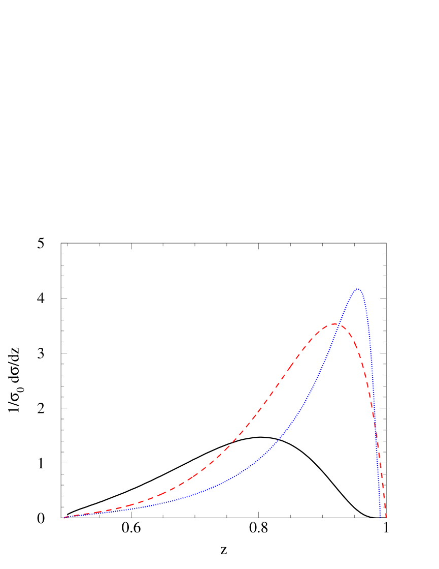
Figure 3: The color-octet contribution at the endpoint normalized to $\sigma_{0}$. The solid line is the perturbative resummation convoluted with the shape function. The dotted line is perturbative resummation only, and the dashed line is no resummation, but including a shape function.

The dashed line is a plot of the shape function alone, and the dotted line includes only the perturbative resummation. Here we use $m_{c}=1.4$ GeV, the one loop coupling constant is evaluated at the hard scale $\mu_{H}=(s/M)(1-r)$, with $\Lambda_{\rm QCD}=190\,{\rm MeV}$, and $a=1$ and $b=2$. The value of the first and second moments of the shape function for this choice of parameters are $890{\rm\ MeV}$ and $(985{\rm\ MeV})^{2}$ respectively. We have chosen the shape function parameters to give a reasonable description of the $p_{\psi}$ distributions measured by BaBar and Belle. Since $m_{c}v^{2}\approx 500$ MeV the moments are consistent with the velocity scaling rules. Fig. 3 gives a picture of the effects of both the perturbative resummation and the shape function. The perturbative resummation gives a result that is highly peaked in the endpoint region. The shape function is also peaked close to the endpoint, though at a lower value, and is broader. It is interesting to note that the convoluted result is broader yet, and its peak is shifted to the left of both the perturbative resummed peak and the shape function peak.

In order to make a consistent comparison of theory to data one needs to treat the endpoint of the color-singlet contribution in SCET and NRQCD. We leave this for future work, and will use the leading order NRQCD calculation of the color-singlet contribution over the full range of momenta. In Fig. 4 we show the sum of the color-octet and color-singlet contributions as the upper line, and the color-singlet contribution only as the lower line. The color-octet matrix elements which set the normalization are chosen to be $\langle{\cal O}^{\psi}_{8}(^{1}S_{0})\rangle=\langle{\cal O}^{\psi}_{8}(^{3}P_{0})\rangle/m_{c}^{2}=1.3\times 10^{-1}{\rm\ GeV}^{3}$. This is plotted against the BaBar data Aubert:2001pd .

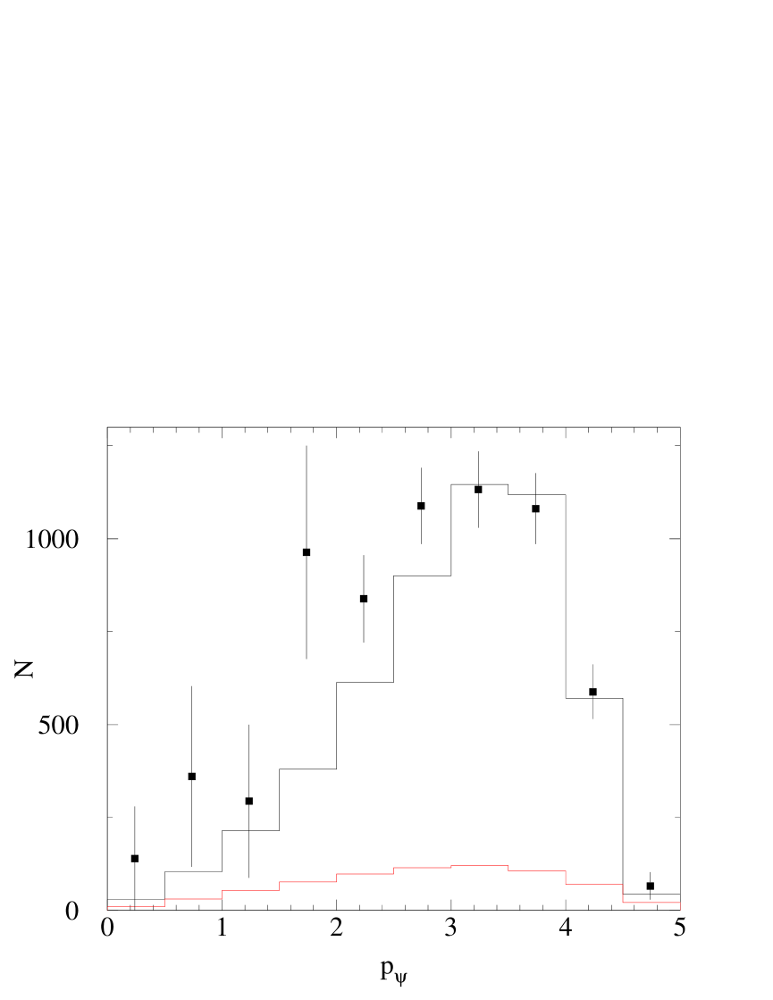
Figure 4: The sum of the color-octet and color-singlet contributions are plotted as the upper line. The lower line is the color-singlet contribution only, and the data are from the BaBar collaboration Aubert:2001pd .

In Fig. 5 we show the same comparison to the Belle data Abe:2001za . The shape function parameters are the same, only the color-octet matrix elements are smaller: $\langle{\cal O}^{\psi}_{8}(^{1}S_{0})\rangle=\langle{\cal O}^{\psi}_{8}(^{3}P_{0})\rangle/m_{c}^{2}=6.6\times 10^{-2}{\rm\ GeV}^{3}$. These values of the color-octet matrix elements are consistent with data from photo- and hadroproduction mefit .

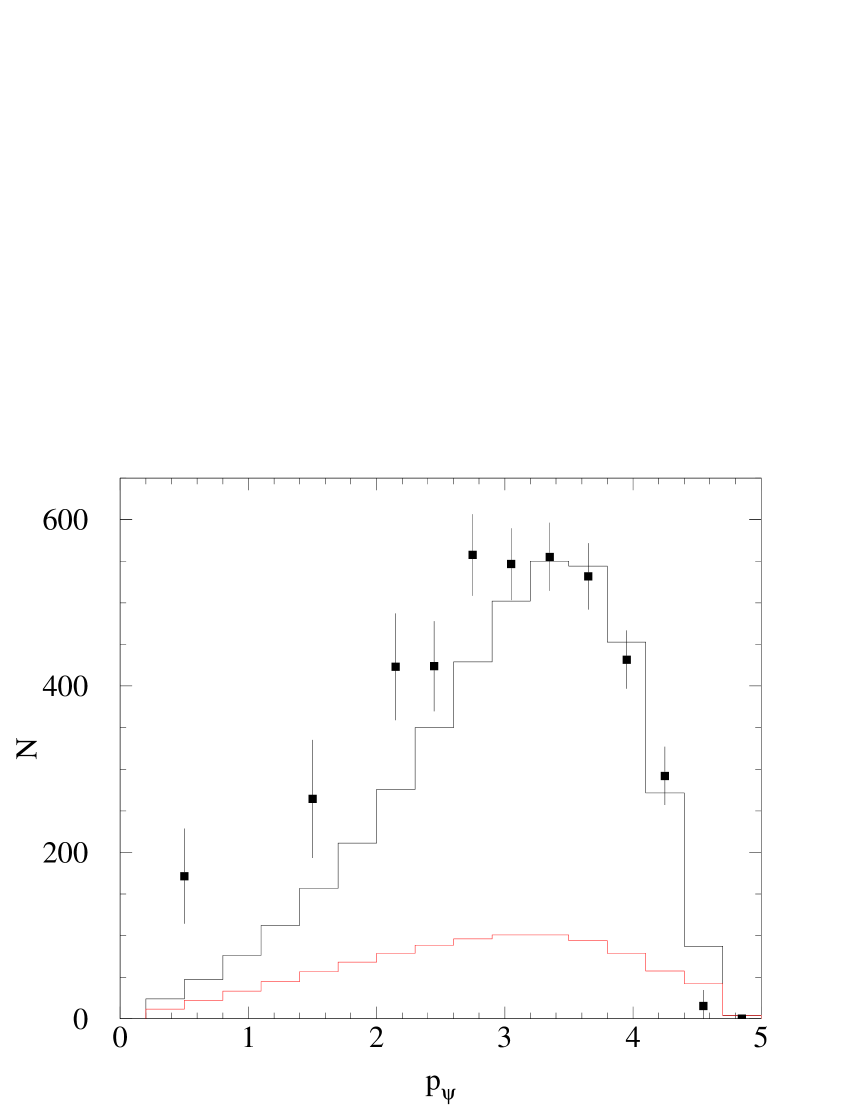
Figure 5: The sum of the color-octet and color-singlet contributions are plotted as the upper line. The lower line is the color-singlet contribution only, and the data are from the Belle collaboration Abe:2001za .

Figs. 4 and 5 concisely present the central point of this work: when perturbative logarithms are resummed and the non-perturbative shape function is included the color-octet contribution becomes a broad distribution as a function of the $J/\psi$ momentum. Furthermore, for a reasonable choice of parameters including the color-octet contribution gives a fairly good description of the $p_{\psi}$ distribution. The color-singlet contribution alone cannot describe the data on $J/\psi$ production at BaBar and Belle.

The effect of the resummation on the angular distibution of the $J/\psi$ is shown in Fig. 6 where we plot $A(p_{\psi})$. The circles with error bars are data from Belle Abe:2001za while the triangles with error bars are data from BaBar Aubert:2001pd . Note that the central value of one data point lies outside the physical range, $-1\leq A(p_{\psi})\leq 1$. The solid line is the color-singlet prediction and the shaded band includes the resummed color-octet contribution. The color-octet ${}^{1}S_{0}$ production mechanism gives $A=1$ while the ${}^{3}P_{J}$ mechanisms gives $A\approx 0.7$. The band shown in Fig. 6 is obtained by varying the two matrix elements $\langle{\cal O}^{\psi}_{8}(^{1}S_{0})\rangle$ and $\langle{\cal O}^{\psi}_{8}(^{3}P_{0})\rangle$ subject to the constraint that both matrix elements are positive and that

$$\langle{\cal O}^{\psi}_{8}(^{1}S_{0})\rangle+3.8\langle{\cal O}^{\psi}_{8}(^{3}P_{0})\rangle/m_{c}^{2}=3.2\times 10^{-2}{\rm\ GeV}^{3},$$ (47)

which is the normalization of the curve shown in Fig. 5. If the normalization in Fig. 4 is used instead, the prediction for $A(p_{\psi})$ is basically the same. The resummed color-octet contributions give $A(p_{\psi})\approx 1$ for nearly the entire $p_{\psi}$ range. This is because for our choice shape function parameters the color-octet dominates color-singlet over the entire range of $p$. The resummed color-octet calculation agrees with the Belle data as well as the BaBar measurement for $p_{\psi}>3.5$ GeV. However, the BaBar measurement for $p_{\psi}<3.5$ GeV is about 2$\sigma$ below theory.

Note that the factorization theorem we derive in this paper is only valid in the endpoint region and the predictions in the region $p_{\psi}<2$ GeV should not be taken too seriously. The effects that are being resummed are no longer dominant in this region and other color-octet production mechanisms may be important. On the other hand, the small value of $A(p_{\psi})$ could indicate the color-octet shape function we are using is too broad and some other mechanism accounts for the observed $J/\psi$ production at these lower values of $p_{\psi}$.

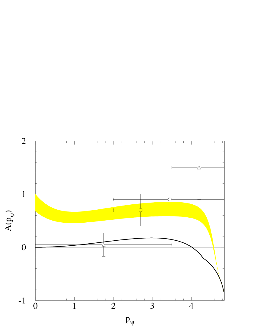
Figure 6: The angular distribution variable $A(p_{\psi})$. The circles represent data from Belle Abe:2001za and the triangle data from BaBar Aubert:2001pd . The solid line is the color-singlet contirbution alone while the shaded band includes the resummed color-octet contribution.

Though the results presented here give a fair description of the $p_{\psi}$ distribution, the Belle collaboration finds that roughly 60% of the cross section comes from the production of a $J/\psi$ in association with another $c\bar{c}$ pair. The theoretical prediction is that this contribution is less than 10% of the cross section. Clearly we do not resolve this issue here, and the mechanism responsible for the copious production of $J/\psi+D\bar{D}$ must be understood before any measurements of the octet shape function parameters can be made at BaBar or Belle.

V Conclusion

Leading order NRQCD calculations of the $J/\psi$ spectrum in NRQCD predict an enhancement at maximal energy due to color-octet contributions. Furthermore, the angular dependence of the $J/\psi$ production due to color-octet contributions is markedly different than the color-singlet. Recent experimental investigations Abe:2001za ; Aubert:2001pd of $e^{+}e^{-}\to J/\psi+X$ are at odds with the leading order predictions. Large Sudakov logarithms appear in the higher order corrections to the color-octet production mechanism which invalidate the perturbative expansion. In addition, as pointed out by Beneke, Rothstein, and Wise Beneke:1997qw , the nonperturbative $v^{2}$ expansion of NRQCD also breaks down at the endpoint, which necessitates the introduction of nonperturbative shape functions to resum these large corrections.

We have studied the color-octet contribution to $e^{+}e^{-}\to J/\psi+X$ using SCET coupled to NRQCD. First we showed how the differential rate factorizes into a hard coefficient, a jet function containing collinear degrees of freedom, and a shape function. The renormalization group equations of SCET were used to move all large logarithms out of operators and into coefficient functions. This allowed the resummation of leading and next-to-leading Sudakov logarithms, and naturally introduced the shape function into the differential spectrum. While previous calculations of Sudakov logarithms in SCET have employed a two-step evolution, we did a one-step evolution, similar to the velocity renormalization group in NRQCD Luke:2000kz . Due to the factorization of collinear and usoft degrees of freedom Bauer:2001yt , these two methods give identical results at leading order in the SCET power counting.

Unfortunately, the shape functions for $J/\psi$ production are not known, so our calculation is not predictive. In the future it may be possible to extract the shape functions from either this spectrum, or from photo- or electroproduction, to be used as input in an analysis of one of the other processes. Until that time, the best we can do is to make a phenomenological model. We are guided in this effort by knowledge of the scalings of the moments of the shape function, which are given by NRQCD power counting rules.

Using a simple model, we can obtain a qualitative feeling for the effects of the perturbative and nonperturbative resummations. We found that both the perturbative resummation or the inclusion of a shape function cause the differential spectrum to be lowered and shifted to smaller energies. Together, the spectrum is very broad, extending the color-octet contribution to very low energies. Qualitatively, this could improve agreement with experimental data for the total rate, the $p_{\psi}$ distribution, and the angular dependence of the spectrum. However, there are still many puzzles with the $J/\psi$ data, in particular the large cross section for $J/\psi$ produced along with open charm and the exclusive double charmonium production Abe:2002rb , both of which exceed existing theoretical estimates. In addition, there are discrepancies between the existing measurements by Belle and BaBar regarding the overall normalization of the cross section as well as the polarization of the $J/\psi$ at largest values of $p_{\psi}$. These discrepancies must be resolved and an understanding of the production mehanism which gives rise to the large $J/\psi c\bar{c}$ cross section is needed before color-octet shape functions can be reliably extracted from the data.

Appendix A Deriving Factorization Theorem for the Endpoint

In this Appendix we show that the rate $e^{+}e^{-}\to J/\psi+X$ in the endpoint region can be factored into a hard coefficient, a jet function, and a shape function. The jet and shape function involve only collinear and usoft fields, respectively. The analysis is similar to the derivation of factorization for $b\to X_{s}\gamma$ Bauer:2001yt ; Bauer:2002nz . We begin by writing the differential cross section as

$$2E_{\psi}\frac{d\sigma}{d^{3}p_{\psi}} = \frac{e^{2}}{16\pi^{3}s^{3}}L^{\mu\nu}\sum_{X}\langle 0|J^{\dagger}_{\nu}(0)|J/\psi+X\rangle\langle J/\psi+X|J_{\mu}(0)|0\rangle(2\pi)^{4}\delta^{4}(q-p_{\psi}-p_{X})$$ (48)

$$= \frac{e^{2}}{16\pi^{3}s^{3}}L^{\mu\nu}\int d^{4}y\,e^{-iq\cdot y}\sum_{X}\langle 0|J^{\dagger}_{\nu}(y)|J/\psi+X\rangle\langle J/\psi+X|J_{\mu}(0)|0\rangle$$

$$\equiv \frac{e^{2}}{16\pi^{3}s^{3}}L^{\mu\nu}T_{\mu\nu},$$

where the sum includes integration over the phase space of $X$. The lepton tensor is

$$L^{\mu\nu}=p_{1}^{\mu}p_{2}^{\nu}+p_{1}^{\nu}p_{2}^{\mu}-g^{\mu\nu}p_{1}\cdot p_{2},$$ (49)

where $p_{1,2}$ are the momenta of the electron and positron, respectively.

Matching the QCD current $J_{\mu}$ onto SCET operators to leading order in $\lambda$ is discussed in Section II. Note that $J^{\dagger}_{\nu}(y)$ picks up an additional phase due to the field redefinition relating QCD fields and SCET/NRQCD effective theory fields:

$$J^{\dagger}_{\nu}(y)=e^{i(Mv-\bar{\cal P}\,n/2)\cdot y}\left[\psi^{\dagger}_{\bf p}\,\Gamma^{\dagger(8,{}^{1}S_{0})}_{\beta\nu}\,B^{\beta}_{\perp}\,\chi_{-{\bf p}}+\psi^{\dagger}_{\bf p}\,\Gamma^{\dagger(8,{}^{3}P_{J})}_{\beta\nu\sigma\delta}B^{\beta}_{\perp}\Lambda\cdot\widehat{{\bf p}}^{\sigma}\Lambda\cdot\mbox{\boldmath$\sigma$}^{\delta}\chi_{-{\bf p}}\right].$$ (50)

The currents in Eq. (50) are the same that appear in inclusive radiative $\Upsilon$ decay Bauer:2001rh . To lowest order in $\alpha_{s}$, $\Gamma^{\dagger(8,{}^{1}S_{0})}_{\beta\nu}$ is the same as in radiative $\Upsilon$ decay, while $\Gamma^{\dagger(8,{}^{3}P_{J})}_{\beta\nu\sigma\delta}$ is different.

We will only derive the factorization theorem for the ${}^{1}S_{0}$ contribution. The generalization to the ${}^{3}P_{J}$ contribution is straightforward. The ${}^{1}S_{0}$ contribution to the hadronic tensor $T_{\mu\nu}$ can be written as

$$T_{\mu\nu} = \int d^{4}y\,e^{-i\sqrt{s}/2(1-\hat{x}){\bar{n}}\cdot y}\Gamma^{(8,{}^{1}S_{0})}_{\alpha\mu}\Gamma^{\dagger(8,{}^{1}S_{0})}_{\beta\nu}$$ (51)

$$\phantom{\int d^{4}y\,e^{i\sqrt{s}/2(1-x){\bar{n}}\cdot y}}\times\sum_{X}\langle 0|\chi^{\dagger}_{-{\bf p}}B^{\beta}_{\perp}\psi_{\bf p}(y)|J/\psi+X\rangle\langle J/\psi+X|\psi^{\dagger}_{\bf p^{\prime}}B^{\alpha}_{\perp}\chi_{-{\bf p^{\prime}}}(0)|0\rangle$$

$$\equiv \Gamma^{(8,{}^{1}S_{0})}_{\alpha\mu}\Gamma^{\dagger(8,{}^{1}S_{0})}_{\beta\nu}T^{\beta\alpha}_{\rm eff}.$$

In the exponent of Eq. (51), we have used $\bar{\cal P}B_{\perp}^{\alpha}=-\sqrt{s}(1-r)B_{\perp}^{\alpha}$ so

$$q^{\mu}-Mv^{\mu}+\bar{\cal P}\frac{n^{\mu}}{2}=\sqrt{s}(1-\hat{x})\frac{\bar{n}^{\mu}}{2}-\frac{r\sqrt{s}}{\hat{x}}(1-\hat{x})\frac{n^{\mu}}{2}\,.$$ (52)

The term proportional to $n^{\mu}$ is suppressed by $r\approx 0.08$ and can be neglected. We can now decouple the usoft gluons in $T_{\rm eff}^{\beta\alpha}$ using the field redefinition Bauer:2001yt

$$A^{\mu}_{n,q}=YA^{(0)\mu}_{n,q}Y^{\dagger}\hskip 14.22636pt\to\hskip 14.22636ptW_{n}=YW_{n}^{(0)}Y^{\dagger}\,,$$ (53)

where the first identity implies the second. The collinear fields with the superscript $(0)$ do not interact with usoft fields to lowest order in $\lambda$. After this field redefinition the color-octet ${}^{1}S_{0}$ current becomes

$$\tilde{J}^{\alpha}_{(8,{}^{1}S_{0})}=\psi^{\dagger}_{\bf p}YB^{(0)\alpha}_{\perp}Y^{\dagger}\chi_{-{\bf p}}\,.$$ (54)

The $J/\psi$ does not contain any collinear quanta, so we can write

$$T^{\beta\alpha}_{\rm eff} =$$ (55)

$$\int d^{4}y\,e^{-i\sqrt{s}/2(1-\hat{x}){\bar{n}}\cdot y}\langle 0|\chi^{\dagger}_{-{\bf p}}YT^{A}Y^{\dagger}\psi_{\bf p}(y)\sum_{X_{u}}|J/\psi+X_{u}\rangle\langle J/\psi+X_{u}|\psi^{\dagger}_{\bf p}YT^{A}Y^{\dagger}\chi_{-{\bf p}}(0)|0\rangle$$

$$\phantom{\int d^{4}y\,e^{i\sqrt{s}/2(1-\hat{x}){\bar{n}}\cdot y}}\times\frac{1}{2}\langle 0|{\rm Tr}\left[T^{B}B^{(0)\beta}_{\perp}(y)\right]\sum_{X_{c}}|X_{c}\rangle\langle X_{c}|{\rm Tr}\left[T^{B}B^{(0)\alpha}_{\perp}(0)\right]|0\rangle\,,$$

where $X_{u}$ contains only usoft particles and $X_{c}$ contains collinear particles. This is possible since interpolating fields for all final state particles can be written with either all collinear or all usoft quanta. By introducing an interpolating field, $a_{\psi}$, for the $J/\psi$, we can use the completeness of states in the usoft and collinear sectors to write

$$\sum_{X_{u}}|J/\psi+X_{u}\rangle\langle J/\psi+X_{u}| = a_{\psi}^{\dagger}\sum_{X_{u}}|X_{u}\rangle\langle X_{u}|a_{\psi}=a_{\psi}^{\dagger}a_{\psi},$$ (56)

$$\sum_{X_{c}}|X_{c}\rangle\langle X_{c}| = 1.$$ (57)

Using Eqs. (56) and (57) in Eq. (55), we get

$$T^{\beta\alpha}_{\rm eff} = \frac{1}{2}\int d^{4}y\,e^{-i\sqrt{s}/2(1-\hat{x}){\bar{n}}\cdot y}\langle 0|\chi^{\dagger}_{-{\bf p}}YT^{A}Y^{\dagger}\psi_{\bf p}(y)\,a_{\psi}^{\dagger}a_{\psi}\,\psi^{\dagger}_{\bf p}YT^{A}Y^{\dagger}\chi_{-{\bf p}}(0)|0\rangle$$ (58)

$$\phantom{\frac{1}{2}\int d^{4}y\,e^{i\sqrt{s}/2(1-x){\bar{n}}\cdot y}}\times\langle 0|{\rm Tr}\left[T^{B}B^{(0)\beta}_{\perp}(y)\right]{\rm Tr}\left[T^{B}B^{(0)\alpha}_{\perp}(0)\right]|0\rangle\,.$$

Next it is useful to define the jet and shape functions. The jet function is defined by

$$\langle 0|{\rm Tr}\left[T^{B}B^{(0)\beta}_{\perp}(y)\right]{\rm Tr}\left[T^{B}B^{(0)\alpha}_{\perp}(0)\right]|0\rangle\equiv-\frac{4\pi g_{\perp}^{\alpha\beta}}{s(1+r)}\int\frac{d^{4}k}{(2\pi)^{4}}e^{-ik\cdot y}J({\bar{n}}\cdot p\,n\cdot k+p_{\perp}^{2}).$$ (59)

Note that the jet function is a function of the labels $\bar{n}\cdot p$ and $p_{\perp}$ of the collinear fields in $B_{\perp}^{(0)\alpha}$, and the residual momentum $n\cdot k$. For the process we are interested in $\bar{n}\cdot p=-\bar{n}\cdot p_{X}$ and $p_{\perp}=0$. Since the jet function is independent of $k_{\perp}$ and $\bar{n}\cdot k$, the momentum integration over these components yields $\delta(n\cdot y)$ and $\delta^{2}(y_{\perp})$. The identity (valid for $q_{0}>0$)

$$\int d^{4}y\,e^{iq\cdot y}\,\langle 0\!\!\!\! | \!\!\!\!{\rm Tr}\left[T^{B}B^{(0)\beta}_{\perp}(y)\right]{\rm Tr}\left[T^{B}B^{(0)\alpha}_{\perp}(0)\right]|0\rangle$$ (60)

$$= 2\,{\rm Im}\left[i\int d^{4}y\,e^{iq\cdot y}\,\langle 0|T\left({\rm Tr}\left[T^{B}B^{(0)\beta}_{\perp}(y)\right]{\rm Tr}\left[T^{B}B^{(0)\alpha}_{\perp}(0)\right]\right)|0\rangle\right],$$

shows that the jet function is related to the imaginary part of $T-$ordered products of the composite field $B_{\perp}^{(0)\alpha}$, which is useful for explicit computations.

The shape function is

$$S^{(8,^{1}S_{0})}(\ell^{+}) = \int\frac{dy^{-}}{4\pi}e^{-\frac{i}{2}\ell^{+}y^{-}}\frac{\langle 0|\chi^{\dagger}_{-{\bf p}}YT^{B}Y^{\dagger}\psi_{\bf p}(y^{-})\,a_{\psi}^{\dagger}a_{\psi}\,\psi^{\dagger}_{\bf p}YT^{B}Y^{\dagger}\chi_{-{\bf p}}(0)|0\rangle}{4m_{c}\langle{\cal O}^{\psi}_{8}(^{1}S_{0})\rangle}$$

$$= \frac{\langle 0|\chi^{\dagger}_{-{\bf p}}T^{B}\psi_{\bf p}\,a_{\psi}^{\dagger}a_{\psi}\,\delta(\ell^{+}-in\cdot D)\psi^{\dagger}_{\bf p}T^{B}\chi_{-{\bf p}}|0\rangle}{4m_{c}\langle{\cal O}^{\psi}_{8}(^{1}S_{0})\rangle}\,.$$

The second line of Eq. (A) is most easily derived by evaluating the first expression in $n\cdot A_{us}=0$ gauge (where $Y=Y^{\dagger}=1$), then replacing ordinary derivatives by usoft gauge covariant derivatives to restore usoft gauge invariance. The normalization is defined so that

$$\int d\ell^{+}S^{(8,^{1}S_{0})}(\ell^{+})=\frac{\langle 0|\chi^{\dagger}_{-{\bf p}}T^{B}\psi_{\bf p}\,a_{\psi}^{\dagger}a_{\psi}\,\psi^{\dagger}_{\bf p}T^{B}\chi_{-{\bf p}}|0\rangle}{4m_{c}\langle{\cal O}^{\psi}_{8}(^{1}S_{0})\rangle}=1.$$ (62)

This function depends on the state of the $c\bar{c}$ pair in the $J/\psi$, and thus there will be a different shape function for the ${}^{3}P_{J}^{(8)}$ contribution.

We substitute these expressions into Eq. (58), then use

$$\int\frac{d^{3}p_{\psi}}{2E_{\psi}}(1+\cos^{2}\theta)=\frac{2\pi}{3}{s(1-r^{2})}P[r,z]dz\,,$$ (63)

where $\cos\theta$ is the angle of the $J/\psi$ with the $e^{+}e^{-}$ beam and $P[r,z]=\sqrt{(1+r)^{2}z^{2}-4r}/(1-r)$. Note that $P[r,1]=1$. In the phase space we use the short distance mass $2m_{c}$ not $M_{\psi}$. The result for the differential cross section is

$$\frac{d\sigma^{(8,^{1}S_{0})}}{dz} = \sigma_{0}^{(8,^{1}S_{0})}P[r,z]\int d\ell^{+}S^{(8,^{1}S_{0})}(\ell^{+})J\left(\sqrt{s}(1-r)[\sqrt{s}(1-x+\bar{\Lambda}/M)-\ell^{+}]\right)$$ (64)

$$= \sigma_{0}^{(8,^{1}S_{0})}P[r,z]\int d\hat{\ell}^{+}S^{(8,^{1}S_{0})}(\hat{\ell}^{+})J\left[s(1-r)(1-x+\bar{\Lambda}/M-\hat{\ell}^{+}/M)\right].$$

Here we have used the fact that $d\ell^{+}S^{(8,^{1}S_{0})}(\ell^{+})$ is boost invariant, and

$$p^{\mu}_{X}=\frac{\sqrt{s}}{2}\Bigg{[}\Bigg{(}1-\frac{r}{\hat{x}}\Bigg{)}n^{\mu}+(1-\hat{x})\bar{n}^{\mu}\Bigg{]}-\ell^{\mu}\,,$$ (65)

so

$$p_{X}^{2} = \sqrt{s}\Bigg{(}1-\frac{r}{\hat{x}}\Bigg{)}\left(\sqrt{s}(1-\hat{x})-\ell^{+}\right)$$ (66)

$$= s(1-r)\left(1-x+\frac{\bar{\Lambda}}{M}-\frac{\hat{\ell}^{+}}{M}\right)\,,$$

where $\ell^{+}=\hat{\ell}^{+}x\sqrt{s}/M_{\psi}$. In the last line we have expanded $p_{X}^{2}$ to lowest order in $1-x$ and $\bar{\Lambda}/M$. Finally, writing $z$ in terms of $x$

$$z=\frac{sx+M_{\psi}^{2}/x}{s+M_{\psi}^{2}}\approx 1-\frac{1-r}{1+r}(1-x),$$ (67)

where again we have expanded to lowest order in $1-x$ and $\bar{\Lambda}/M$, and defining

$$\hat{\ell}^{+}=\bar{\Lambda}+M\frac{1+r}{1-r}(1-\xi),$$ (68)

we find $p_{X}^{2}=s(1+r)(\xi-z)$ . The factorization theorem can then be written as

$$\frac{d\sigma^{(8,^{1}S_{0})}}{dz} = \sigma_{0}^{(8,^{1}S_{0})}P[r,z]\,M\frac{1+r}{1-r}\int_{z}^{1}d\xi\,S^{(8,^{1}S_{0})}\left[M\frac{1+r}{1-r}(1-\xi)+\bar{\Lambda}\right]J(s(1+r)(\xi-z))$$ (69)

$$\equiv \sigma_{0}^{(8,^{1}S_{0})}P[r,z]\int_{z}^{1}d\xi\,S^{(8,^{1}S_{0})}(\xi)J(s(1+r)(\xi-z)),$$

where $S^{(8,^{1}S_{0})}$ as a function of $\xi$ is defined such that $\int d\xi{S}^{(8,^{1}S_{0})}(\xi)=1$. The integration limits on $\xi$ are easy to understand: $p_{X}^{2}>0$ requires $\xi>z$ and the upper limit comes from the requirement that $d\sigma/dz$ vanish at the kinematic limit $z=1$.

Appendix B The Jet Function

In this section we discuss the jet function and its renormalization. We show how to renormalize the moments of the jet function and evaluate these moments to $O(\alpha_{s})$. We derive the renormalization group equation (RGE) for the moments needed for the resummation of endpoint logarithms. We will assume that the usoft fields have already been decoupled by the field redefinition, Eq. (53), and will use the superscript $(0)$ to denote bare fields instead.

We can invert Eq. (59) to obtain

$$J(\bar{n}\cdot p\,n\cdot k+p_{\perp}^{2}) = -\frac{s(1+r)}{4\pi}$$

$$\times{\rm Im}\left[i\int d^{4}y\,e^{ik\cdot y}\,\langle 0|T\left({\rm Tr}\left[T^{B}B^{\beta}_{\perp}(y)\right]{\rm Tr}\left[T^{B}B_{\perp\,\beta}(0)\right]\right)|0\rangle\right].$$

To lowest order in $\alpha_{s}$, we replace the $B_{\perp}^{\alpha}$ with $A_{\perp}^{\alpha}$, so up to a numerical factor the jet function is given by the discontinuity of the SCET collinear gluon propagator. Therefore,

$$J(\bar{n}\cdot p\,n\cdot k+p_{\perp}^{2}) = -\frac{s(1+r)}{\pi}\,{\rm Im}\frac{1}{\bar{n}\cdot p\,n\cdot k+p_{\perp}^{2}+i\epsilon}$$

$$= s(1+r)\delta(\bar{n}\cdot p\,n\cdot k+p_{\perp}^{2})$$

$$= \delta(\xi-z)\,.$$

In the last line we have used $p_{X}^{2}=\bar{n}\cdot p\,n\cdot k+p_{\perp}^{2}=s(1+r)(\xi-z)$.

To calculate the renormalization group equations for the moments of the jet function, we begin with the definition in Eq. (B). The moments as defined in Eq. (30) do not correspond to local SCET operators, so it is easiest to compute the time-ordered product to one-loop then take moments of the result. Since the divergence depends on the moment variable, $N$, we need to introduce an $N$ dependent renormalization for the moments of the jet function: $J_{N}=Z_{N}J_{N}^{(0)}$, where $J_{N}^{(0)}$ is the $N$th moment of the bare jet function. The field appearing in the definition of $J_{N}$ is the composite field $B_{\perp}$. For computing the $O(\alpha_{s})$ anomalous dimension one can simply ignore the $Z$ factors for the fields in the Wilson lines since these counterterms will only contribute at $O(\alpha_{s}^{2})$. Therefore, $B_{\perp}=\sqrt{Z_{3}}B^{(0)}_{\perp}$, and

$$J_{N} = -\frac{s(1+r)}{4\pi}Z_{N}Z_{3}$$

$$\times\int_{0}^{1}dz\,z^{N}\,{\rm Im}\left[i\int d^{4}y\,e^{ik\cdot y}\,\langle 0|T\left({\rm Tr}\left[T^{B}B^{(0)\beta}_{\perp}(y)\right]{\rm Tr}\left[T^{B}B^{(0)}_{\perp\,\beta}(0)\right]\right)|0\rangle\right],$$

where $Z_{3}$ is the wavefunction renormalization of the gluon field,

$$Z_{3}=1+\frac{\alpha_{s}}{4\pi}\frac{1}{\epsilon}\left(C_{A}\frac{5}{3}-n_{f}\frac{2}{3}\right).$$ (73)

The $O(\alpha_{s})$ corrections to the time-ordered product are shown in Fig. 7. In addition to the one-loop graphs there are three

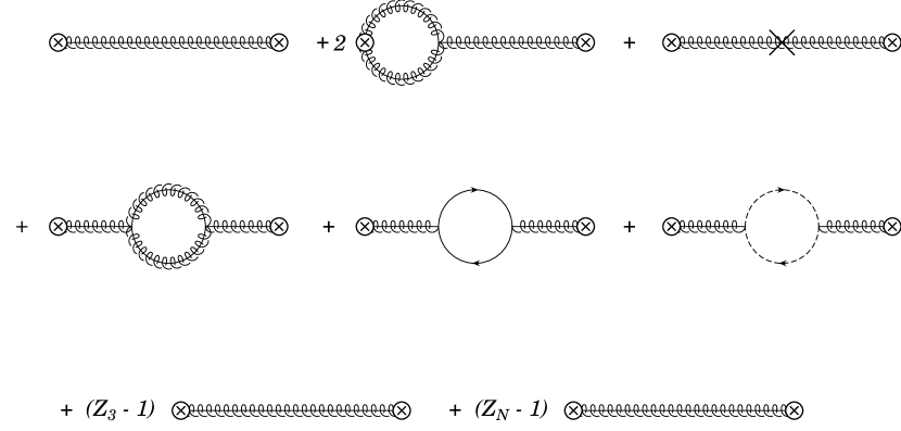
Figure 7: Graphs contributing to $J_{N}$ up to $O(\alpha_{s})$.

counterterm contributions. Two come from the $Z$ factors in Eq. (B) and correspond to the last two diagrams in Fig. 7. There is also a tree level insertion of the $O(\alpha_{s})$ wavefunction counterterm for the collinear gluons, shown as a cross in the third diagram of the first line of Fig. 7. This contribution cancels against the term proportional to $Z_{3}-1$ in the third line of Fig. 7.

Therefore, the divergences from the one-loop graphs must be canceled by the diagram proportonal to $Z_{N}-1$ in the last line of Fig. 7. Evaluation of the graphs and derivation of the renormalization group equation is straightforward. We already calculated the tree-level diagram in Eq. (B) and the self energy corrections are standard. The only remaining graph to calculate is the second diagram in Fig. 7, which has a divergent contribution of

$$-\frac{s(1+r)}{\pi}\int_{0}^{1}dz\,z^{N}\,\frac{\alpha_{s}C_{A}}{2\pi}{\rm Im}\left\{\frac{1}{p_{X}^{2}+i\delta}\left[\frac{2}{\epsilon^{2}}+\frac{1}{\epsilon}\left(1+2\log\frac{\bar{\mu}^{2}}{(-1-i\delta)p_{X}^{2}}\right)\right]\right\}.$$ (74)

Taking the imaginary part, using

$${\rm Im}\left[\frac{1}{p_{X}^{2}+i\delta}\log\frac{\bar{\mu}^{2}}{(-1-i\delta)p_{X}^{2}}\right]=\frac{\pi}{s(1+r)}\left[\frac{1}{(1-z)_{+}}-\delta(1-z)\log\frac{\bar{\mu}^{2}}{s(1+r)}\right],$$ (75)

we can easily integrate over $z$. Setting the divergent part to zero gives

$$Z_{N}-1=-\frac{\alpha_{s}C_{A}}{\pi\epsilon^{2}}-\frac{\alpha_{s}}{2\pi\epsilon}\left(\frac{11C_{A}}{6}-\frac{n_{f}}{3}+2C_{A}\log\frac{\bar{\mu}^{2}N}{s(1+r)N_{0}}\right).$$ (76)

Calculating the anomalous dimension in the usual way, we get Eq. (32) for the renormalization of the jet function. We can also evaluate the one-loop expression for the renormalized jet function from the diagrams in Fig. 7:

$$J_{N}=1+\frac{C_{A}\alpha_{s}}{2\pi}\log^{2}\left(\frac{{\bar{\mu}}^{2}N}{s(1+r)N_{0}}\right)+\frac{\alpha_{s}}{\pi}\left(\frac{11}{12}C_{A}-\frac{1}{6}n_{f}\right)\log\left(\frac{{\bar{\mu}}^{2}N}{s(1+r)N_{0}}\right)+...\,$$ (77)

The ellipsis represents contributions which are not enhanced by large logarithms. Note that the result of explicit evaluation of $J_{N}$ agrees with the solution of the renormalization group equation to $O(\alpha_{s})$. It is clear that the large logs in the moments of the jet function are minimized when ${\bar{\mu}}^{2}=s(1+r)N_{0}/N$.

References

• (1) J. J. Aubert et al., Phys. Rev. Lett.  33, 1404 (1974); J. E. Augustin et al., Phys. Rev. Lett.  33, 1406 (1974).
• (2) G. T. Bodwin, E. Braaten and G. P. Lepage, Phys. Rev. D 51, 1125 (1995) [Erratum-ibid. D 55, 5853 (1995)].
• (3) M. E. Luke, A. V. Manohar and I. Z. Rothstein, Phys. Rev. D 61, 074025 (2000).
• (4) R. Barbieri, R. Gatto and E. Remiddi, Phys. Lett. B 61, 465 (1976); Phys. Lett. B 106, 497 (1981); R. Barbieri, M. Caffo, R. Gatto and E. Remiddi, Nucl. Phys. B 192, 61 (1981).
• (5) G. T. Bodwin, E. Braaten and G. P. Lepage, Phys. Rev. D 46, 1914 (1992).
• (6) E. Braaten and S. Fleming, Phys. Rev. Lett.  74, 3327 (1995); P. L. Cho and A. K. Leibovich, Phys. Rev. D 53, 150 (1996); Phys. Rev. D 53, 6203 (1996).
• (7) G. T. Bodwin, hep-ph/0212203.
• (8) P. L. Cho and M. B. Wise, Phys. Lett. B 346, 129 (1995); A. K. Leibovich, Phys. Rev. D 56, 4412 (1997); M. Beneke and M. Kramer, Phys. Rev. D 55, 5269 (1997); E. Braaten, B. A. Kniehl and J. Lee, Phys. Rev. D 62, 094005 (2000).
• (9) T. Affolder et al. [CDF Collaboration], Phys. Rev. Lett.  85, 2886 (2000).
• (10) K. Abe et al. [BELLE Collaboration], Phys. Rev. Lett.  88, 052001 (2002).
• (11) B. Aubert et al. [BABAR Collaboration], Phys. Rev. Lett.  87, 162002 (2001).
• (12) E. Braaten and Y. Q. Chen, Phys. Rev. Lett.  76, 730 (1996).
• (13) P. L. Cho and A. K. Leibovich, Phys. Rev. D 54, 6690 (1996).
• (14) F. Yuan, C. F. Qiao and K. T. Chao, Phys. Rev. D 56, 321 (1997).
• (15) S. Baek, P. Ko, J. Lee and H. S. Song, J. Korean Phys. Soc.  33, 97 (1998).
• (16) G. A. Schuler, Eur. Phys. J. C 8, 273 (1999).
• (17) M. Beneke, G. A. Schuler and S. Wolf, Phys. Rev. D 62, 034004 (2000).
• (18) K. Abe et al. [Belle Collaboration], Phys. Rev. Lett.  89, 142001 (2002)
• (19) A. V. Luchinsky, hep-ph/0301190; G. T. Bodwin, J. Lee and E. Braaten, Phys. Rev. D 67, 054023 (2003); Phys. Rev. Lett.  90, 162001 (2003); K. Y. Liu, Z. G. He and K. T. Chao, Phys. Lett. B 557, 45 (2003); E. Braaten and J. Lee, Phys. Rev. D 67, 054007 (2003); S. J. Brodsky, A. S. Goldhaber and J. Lee, hep-ph/0305269; B. L. Ioffe and D. E. Kharzeev, hep-ph/0306062.
• (20) J. H. Kuhn and H. Schneider, Phys. Rev. D 24, 2996 (1981); Z. Phys. C 11, 263 (1981); V. M. Driesen, J. H. Kuhn and E. Mirkes, Phys. Rev. D 49, 3197 (1994); L. Clavelli, Phys. Rev. D 26, 1610 (1982).
• (21) M. Beneke, I. Z. Rothstein and M. B. Wise, Phys. Lett. B 408, 373 (1997).
• (22) C. W. Bauer, S. Fleming and M. Luke, Phys. Rev. D 63, 014006 (2001).
• (23) C. W. Bauer, S. Fleming, D. Pirjol and I. W. Stewart, Phys. Rev. D 63, 114020 (2001).
• (24) C. W. Bauer and I. W. Stewart, Phys. Lett. B 516, 134 (2001).
• (25) C. W. Bauer, D. Pirjol and I. W. Stewart, Phys. Rev. D 65, 054022 (2002).
• (26) C. W. Bauer, C. W. Chiang, S. Fleming, A. K. Leibovich and I. Low, Phys. Rev. D 64, 114014 (2001).
• (27) A. V. Manohar, T. Mehen, D. Pirjol and I. W. Stewart, Phys. Lett. B 539, 59 (2002).
• (28) D. Pirjol and I. W. Stewart, Phys. Rev. D 67, 094005 (2003).
• (29) G. P. Korchemsky and A. V. Radyushkin, Sov. J. Nucl. Phys.  45, 127 (1987) [Yad. Fiz.  45, 198 (1987)]; G. P. Korchemsky and G. Marchesini, Nucl. Phys. B 406, 225 (1993) [arXiv:hep-ph/9210281].
• (30) A. K. Leibovich, I. Low and I. Z. Rothstein, Phys. Rev. D 61, 053006 (2000).
• (31) A. K. Leibovich, I. Low and I. Z. Rothstein, Phys. Lett. B 513, 83 (2001).
• (32) G. P. Korchemsky and G. Sterman, Phys. Lett. B 340, 96 (1994); R. Akhoury and I. Z. Rothstein, Phys. Rev. D 54, 2349 (1996).
• (33) S. Fleming and A. K. Leibovich, Phys. Rev. D 67, 074035 (2003).
• (34) S. Fleming and A. K. Leibovich, Phys. Rev. Lett.  90, 032001 (2003).
• (35) A. V. Manohar, J. Soto and I. W. Stewart, Phys. Lett. B 486, 400 (2000).
• (36) A. K. Leibovich, Z. Ligeti and M. B. Wise, Phys. Lett. B 539, 242 (2002).
• (37) M. Beneke and I. Z. Rothstein, Phys. Rev. D 54, 2005 (1996) [Erratum-ibid. D 54, 7082 (1996)]; J. Amundson, S. Fleming and I. Maksymyk, Phys. Rev. D 56, 5844 (1997).
• (38) C. W. Bauer, S. Fleming, D. Pirjol, I. Z. Rothstein and I. W. Stewart, Phys. Rev. D 66, 014017 (2002).
• (39) A. K. Leibovich, Z. Ligeti and M. B. Wise, hep-ph/0303099.
• (40) K. m. Cheung, W. Y. Keung and T. C. Yuan, Phys. Rev. Lett.  76, 877 (1996); P. L. Cho, Phys. Lett. B 368, 171 (1996); C. G. Boyd, A. K. Leibovich and I. Z. Rothstein, Phys. Rev. D 59, 054016 (1999).