HD-THEP-02-35

hep-ph/0306137

The Odderon in Quantum Chromodynamics

Carlo Ewerz

Institut für Theoretische Physik, Universität Heidelberg
Philosophenweg 16, D-69120 Heidelberg, Germany
         
email: carlo@thphys.uni-heidelberg.de

The Odderon is the leading exchange in hadronic scattering processes at high energies in which negative charge conjugation and parity quantum numbers are transferred in the $t$-channel. We review the origin of the Odderon in Regge theory, its status in perturbative and nonperturbative Quantum Chromodynamics, as well as its phenomenology.

1 Introduction

Quantum Chromodynamics (QCD) is one of the cornerstones of the Standard Model of particle physics. It is the gauge theory of color charges describing the interactions of quarks and gluons. By now it is beyond any reasonable doubt that QCD is the correct microscopic theory of the strong interaction. Quarks and gluons interact strongly at large distances which makes it intrinsically difficult to calculate observables in QCD to a high precision. Therefore the experimental tests of QCD remained on a qualitative level for quite some time. The last decade has seen steady progress in the area of calculational techniques and many aspects of QCD have since been tested experimentally at a really quantitative level of a few per cent. We have thus entered an era of precision tests of QCD. It can be considered a great success of QCD that it has passed all these tests. Moreover, the investigation of QCD has taught us a lot about quantum field theory in general. QCD is thus not only interesting from a phenomenological point of view but also because it can serve as a model field theory which exhibits an amazingly rich structure.

Despite the enormous success of QCD there remains a number of deep questions to be answered in the field of strong interaction physics. The most fundamental problem is why quarks and gluons cannot be observed as free particles and how exactly they form the observable hadronic bound states. A slightly less fundamental but equally challenging problem is to understand the high energy behavior of hadronic scattering processes. The Regge limit of large center–of–mass energy and small momentum transfer attracted a lot of interest already long before the advent of QCD. In pre–QCD times Regge theory was developed and successfully applied to high energy scattering. The findings of Regge theory in fact belong to the deep truths of high energy physics. Regge theory is based on a few fundamental assumptions about the scattering amplitude like unitarity and analyticity. The interaction of the colliding particles is interpreted in terms of exchanges between them corresponding to so–called Regge poles and Regge cuts. At large center–of–mass energy $\sqrt{s}$ the leading contribution is given by the exchange of the Pomeron (or Pomeranchuk pole) which carries vacuum quantum numbers, in particular positive charge parity $C=+1$. This exchange was found to result in a slow growth of cross sections with energy, $\sigma\sim s^{\alpha_{\mbox{\tiny{\rm I\kern-1.25ptP}}}-1}$, with the Pomeron intercept $\alpha_{\mbox{\scriptsize{\rm I\kern-1.75ptP}}}\simeq 1.08$. In the 1960’s a field theory of interacting Pomerons was formulated and widely studied. After the discovery of QCD in 1973 the interest shifted somewhat away from Regge theory towards hard scattering processes which due to asymptotic freedom can be described in perturbative QCD. The interest in the Regge limit was revived during the last decade by new experimental data obtained at the HERA collider at DESY. Now the main focus is on attempts to derive Regge theory from the underlying dynamics of QCD, i. e. in terms of quarks and gluons. Although remarkable progress has been made, we are still far from a full understanding of the high energy limit of QCD.

It was for a long time assumed that the cross sections for particle and antiparticle scattering become equal at very high energies, for example for proton–proton and antiproton–proton scattering. This became widely known as the Pomeranchuk theorem [1]. Already in 1970 the possibility of processes violating the Pomeranchuk theorem was discussed, and the corresponding amplitudes were studied in detail for the case of asymptotically constant cross sections. Motivated by the experimental observation of rising cross sections at the highest available energies Łukaszuk and Nicolescu [2] in 1973 considered this possibility also in the case of asymptotically rising cross sections and established the concept of a Regge exchange with an intercept close to one which – in contrast to the Pomeron – carries odd charge parity $C=-1$. Accordingly, the name Odderon was coined for this exchange in [3]. The Odderon has experienced a quite varied history. It was soon shown that the possible existence of the Odderon does not contradict the fundamental theorems of Regge theory as was previously often assumed. Nevertheless, the Odderon was for a long time widely considered a doubtful concept. Even if its existence was possible it was thought not to exist or at least to be of little importance in reality. This scepticism was supported by the experimental results which showed only little evidence for the Odderon. The search concentrated on finding differences between particle cross sections and the corresponding antiparticle cross sections at high energy. Since the Odderon couples differently to particles and antiparticles due to its negative charge parity such differences would indicate an Odderon exchange. The only trace of the Odderon was found in a small difference of the elastic proton–proton and proton–antiproton differential cross sections. Unfortunately, the statistics of the $p\bar{p}$ data was low and the results were thus not unambiguous. Other hints were even less convincing and seemed to be rather controversial.

Today the experimental evidence for the Odderon is still very unsatisfactory, the best sign still being the difference in the differential cross sections for elastic $pp$ and $p\bar{p}$ scattering measured at the CERN Intersecting Storage Rings (ISR). But the theoretical perspective on the Odderon has changed completely. Instead of being thought of as a doubtful concept the Odderon is now considered a firm prediction of QCD. Our QCD–motivated picture of high energy scattering is largely based on gluon exchange, the Pomeron being a mainly gluonic object which in the simplest picture is composed of two gluons in a colorless state. Although nonperturbative effects necessarily play an important rôle this picture is well established also experimentally. From this point of view it would be very surprising if the exchange of three gluons in a colorless $C=-1$ state, i. e. an Odderon, would not exist. Formally, this picture was supported by the investigation of the Regge limit in perturbative QCD: In 1980 the existence of a colorless three–gluon exchange at high energies with negative charge parity was established by Bartels [4], Jaroszewicz [5], and Kwieciński and Praszałowicz [6]. But even after that it took almost twenty years before the corresponding intercept $\alpha_{\mbox{\scriptsize{\rm\kern 1.68004pt\vrule width=0.14003pt,height=4.37012pt,depth=-0.1507pt\kern-1.81996ptO}}}$ was shown to be close to one, thus proving the existence of an Odderon at least in perturbative QCD. In addition to this important result the investigation of the Odderon in perturbative QCD has led to the discovery of beautiful and unexpected relations of high energy QCD to the theory of integrable models. In this respect the Odderon turned out to be a highly interesting object also from a theoretical point of view.

The rapid progress in the study of the perturbative Odderon was in the last few years paralleled by a new development in the phenomenology of the Odderon. Earlier investigations had mainly concentrated on processes in which the Odderon exchange gives one of several contributions to the cross section. The corresponding predictions were often plagued by the large uncertainties due to the unknowns of the other possible exchanges. Now the interest has shifted towards more exclusive processes in which the Odderon is the only possible exchange, typically with the exception of an additional photon contribution which is theoretically well under control. Hence already the observation of such processes would clearly indicate the existence of the Odderon. A typical example of such processes is the diffractive production of pseudoscalar mesons in electron–proton scattering at high energy. The photon which is radiated off the electron carries negative charge parity. The positive charge parity of the pseudoscalar meson thus requires a colorless $C=-1$ exchange producing a rapidity gap between the meson and the proton, hence an Odderon. The first experimental study [7] of this process has just been performed by the H1 collaboration at the DESY HERA collider, and further results are expected for the near future. Similar diffractive processes have also been proposed in other reactions like proton–(anti)proton collisions or photon–photon scattering at high energies. The expected cross sections for many of these processes are in a range which should make it possible to find the Odderon and to study its properties at current and future accelerators.

The high energy limit of QCD has in the recent past attracted much interest in a wider context and is presently a field in rapid development. At high energies the quarks and gluons inside the colliding hadrons form a very dense system which is largely dominated by nonperturbative effects. When probed with sufficiently high momentum, however, the partons interact only weakly. QCD matter under these conditions has recently been termed a color glass condensate: colored partons are in a very dense state that resembles a glass because its quantum fluctuations are frozen over rather long timescales in a frame in which the colliding hadrons move very fast. It is expected that such a system exhibits new and very interesting phenomena. Although the partons interact only weakly the usual methods of fixed order perturbation theory cannot be applied because of the density of the system. Of particular importance is the effect of recombinations of different parton cascades in the hadrons. Such effects will eventually also tame the growth of hadronic cross sections which according to unitarity can at most be logarithmic in the high energy limit. To understand the details of unitarity restoration poses a big challenge. New techniques and different approaches to this problem are currently developed. Many of them lead to similar results corresponding to the perturbative Pomeron when the limit of low densities is taken. It will therefore be very important to determine and understand the characteristic differences between these approaches by going beyond the simplest case of two–gluon exchange. It is very likely that the study of the Odderon will be very helpful in this context. Although being a more theoretical aspect this issue is certainly very important for a full understanding of QCD in the high energy limit.

It is the aim of this article to review the present status of the Odderon from a theoretical as well as from a phenomenological perspective. We will especially emphasize the importance of the recent developments regarding the perturbative description of the Odderon and of the new strategies in its phenomenology. It is our strong belief that these aspects offer the most promising possibilities for further progress in the near future. We start by giving a brief introduction to Regge theory in section 2 where we discuss in particular the asymptotic theorems and their relevance to the Odderon. We then turn to the theoretical aspects of the Odderon in section 3. A large portion of that section is devoted to the Odderon in perturbative QCD. The discussion of this subject is facilitated by some familiarity with the perturbative description of the Pomeron of which we present the relevant aspects. We then proceed to the Bartels–Kwieciński–Praszałowicz (BKP) equation describing the perturbative Odderon and explain its relation to integrable models. We present the known solutions to the BKP equation and discuss the important question of the Odderon intercept. Also in that section we discuss which rôle the Odderon plays in the more general context of high energy QCD. We conclude the section with a discussion of some results and ideas concerning nonperturbative aspects of the Odderon. Section 4 deals with the phenomenology of the Odderon. After presenting general considerations we discuss in some detail the experimental evidence for the Odderon as it is found in the differential cross sections for elastic $pp$ and $p\bar{p}$ scattering. We then proceed to review the different observables which have been proposed for observing the Odderon and describe their advantages and the uncertainties involved in the corresponding theoretical predictions. Finally, we present our conclusions and some possible directions for further study.

The choice of the material covered in this review is influenced by my own interests and prejudices, and by the will to keep the review finite. I still hope that my attempts at giving fair mention to the relevant contributions to the field have not failed too badly. I apologize to all those whose important work is not adequately represented.

2 Pomeron and Odderon in Regge Theory

The Odderon as well as the Pomeron are objects which originate in Regge theory. We will therefore give a brief account of the basic concepts of Regge theory, with particular emphasis on those issues that are directly relevant to the physics of the Odderon. We will then briefly discuss the basic theorems of Regge theory and some aspects of the Pomeron. Finally, we describe which place the Odderon finds in Regge theory. In particular, we will describe the so–called maximal Odderon, that is the maximal energy dependence that the Odderon can have without violating the Pomeranchuk theorem.

It should be pointed out that the main focus of the present review is on the more recent development related to the Odderon, namely its nature in perturbative QCD and its phenomenology which will be discussed in the subsequent sections. In favor of those aspects we concentrate on the essential issues only in the present section on Regge theory – despite the great importance that Regge theory has had, and still has, for the understanding of high energy scattering and for the development of the concept of the Odderon. Therefore no attempt on completeness is made. For detailed accounts of Regge theory we refer the reader to [8]-[11].

2.1 Regge Theory and the Pomeron

Already before the advent of QCD, hadronic scattering processes at high center–of–mass energy were successfully described in the framework of Regge theory. More specifically, Regge theory is designed to describe scattering processes at high center–of–mass energy $\sqrt{s}$ much larger than the momentum transfer $\sqrt{-t}$ in the reaction. The latter is supposed to be of the order of some hadronic mass scale $m_{H}$,

$$s\gg|t|\simeq m_{H}^{2}\,.$$ (2.1)

This limit is known as the Regge limit. Regge theory is based on very general properties of the scattering matrix, namely its Lorentz invariance, its unitarity, and its analyticity. The latter postulate determines also the properties of the scattering matrix under the crossing of initial and final state particles. The basic object of interest in Regge theory is the scattering amplitude $A$. For a two–to–two scattering process $a+b\to c+d$, it is pictorially given by

(2.2)

It depends on two of the three Mandelstam variables $s,t,u$ defined by the momenta $p_{i}$ of the four particles as

$$s = (p_{a}+p_{b})^{2}$$ (2.3)

$$t = (p_{a}-p_{c})^{2}$$ (2.4)

$$u = (p_{a}-p_{d})^{2}\,,$$ (2.5)

which are related via

$$s+t+u=\sum_{i=a}^{d}m_{i}^{2}\,.$$ (2.6)

One usually chooses as variables the squared center–of–mass energy $s$ and the squared momentum transfer $t$, and hence considers the scattering amplitude $A(s,t)$. The total cross section is related to the elastic forward scattering amplitude $A(s,t=0)$ via the optical theorem

$$\sigma_{T}=\frac{1}{s}\,\mbox{Im}\,A_{\mbox{\scriptsize el}}(s,t=0)\,.$$ (2.7)

Another observable of interest is the differential cross section $d\sigma/dt$ which is obtained from the scattering amplitude via

$$\frac{d\sigma}{dt}=\frac{1}{16\pi s^{2}}\,|A(s,t)|^{2}\,.$$ (2.8)

The scattering amplitude can be written in a $t$-channel partial wave expansion

$$A(s,t)=16\pi\sum_{l=0}^{\infty}(2l+1)A_{l}(t)P_{l}(z_{t})$$ (2.9)

with the Legendre polynomials $P_{l}$ and

$$z_{t}=1+\frac{2s}{t-4m^{2}}\simeq 1+\frac{2s}{t}\,,$$ (2.10)

where we have neglected the masses of the scattering particles in the last step. The $A_{l}(t)$ are called the partial waves. One then applies the Sommerfeld–Watson transformation to write the scattering amplitude as an integral over the $t$-channel angular momentum $l$ which is understood now as a complex variable,

$$A(s,t)=\frac{1}{2i}\int_{C}dl(2l+1)\frac{A(l,t)}{\sin\pi l}P(l,z_{t})\,.$$ (2.11)

The contour $C$ surrounds the real axis from $0$ to $\infty$. The Legendre polynomials $P_{l}$ have a natural analytic continuation to complex $l$, $P_{l}(z_{t})\to P(l,z_{t})$ when they are written in terms of hypergeometric functions. In addition, one has to find an analytic continuation $A(l,t)$ of the functions $A_{l}$. In order to find a unique continuation of these one has to impose a large $|l|$ behavior in the complex $l$-plane. It turns out that this is not possible for a single function $A(l,t)$. Instead one has to introduce signatured partial wave amplitudes $A^{(+1)}(l,t)$ and $A^{(-1)}(l,t)$ that are the analytic continuations for even and odd partial wave amplitudes, respectively. The Sommerfeld–Watson integral then becomes

$$A(s,t)=\frac{1}{2i}\int_{C}dl\frac{(2l+1)}{\sin\pi l}\sum_{\eta=\pm 1}\frac{\eta+e^{-i\pi l}}{2}\,A^{(\eta)}(l,t)P(l,z_{t})\,,$$ (2.12)

where $\eta=\pm 1$ is called the signature of the partial wave. We now deform the contour $C$ to a contour $C^{\prime}$ that runs parallel to the imaginary axis with $\mbox{Re}\,{l}=-1/2$. In general the function $A^{(\eta)}(l,t)$ may have singularities in the complex $l$-plane, for example simple poles situated at $l=\alpha^{(\eta)}_{i}(t)$. For the moment we will consider only simple poles, but will discuss other types of singularities later. When deforming the contour $C$ to $C^{\prime}$ we collect $2\pi i$ times the residue of a pole when the contour crosses it. Accordingly, we get

$$A(s,t) = \frac{1}{2i}\int_{-\frac{1}{2}-i\infty}^{-\frac{1}{2}+i\infty}dl\frac{(2l+1)}{\sin\pi l}\sum_{\eta=\pm 1}\frac{\eta+e^{-i\pi l}}{2}\,A^{(\eta)}(l,t)P(l,z_{t})$$ (2.13)

$$+\sum_{\eta=\pm 1}\sum_{i}\frac{\eta+e^{-i\pi\alpha^{(\eta)}_{i}(t)}}{2}\frac{\tilde{\beta}^{(\eta)}_{i}(t)}{\sin\pi\alpha^{(\eta)}_{i}(t)}P(\alpha^{(\eta)}_{i}(t),z_{t})\,.$$

The $\tilde{\beta}^{(\eta)}_{i}(t)$ are $\pi(2\alpha^{(\eta)}_{i}(t)+1)$ times the residues of the poles. The simple poles are called Regge poles with signature $\eta$. It turns out that the remaining integral in the first line of (2.13) vanishes in the limit $s\gg|t|$ due to the behavior of the Legendre polynomials in this limit. Using that behavior one can also simplify the second line in (2.13) and obtains for the amplitude

$$A(s,t)=\sum_{\eta=\pm 1}\sum_{i}A_{i}^{(\eta)}(s,t)\,,$$ (2.14)

and $A_{i}^{(\eta)}$ denotes the contribution of a pole of signature $\eta$ located at $\alpha_{i}(t)$. Its contribution to $A(s,t)$ is (dropping the index $i$)

$$A^{(\eta)}(s,t)=\beta^{(\eta)}(t)\,\Gamma(-\alpha^{(\eta)}(t))\,\eta\,\xi^{(\eta)}(t)\left(\frac{s}{s_{0}}\right)^{\alpha^{(\eta)}(t)}\,,$$ (2.15)

where $\Gamma$ is the Euler gamma function. The factors

$$\xi^{(\pm 1)}(t)=1\pm e^{-i\pi\alpha(t)}$$ (2.16)

are called signature factors. In eq. (2.15) we have for simplicity absorbed several $t$-dependent factors into the factor $\beta$. It can be shown that the $\beta(t)$ are real–valued and contain as one factor the residue of the pole. In addition we have introduced a scale $s_{0}$ with respect to which the squared energy $s$ is measured. A priori $s_{0}$ cannot be fixed, often one chooses $s_{0}=1\,\mbox{GeV}^{2}$. Note that instead of $l$ one often uses $\omega$ or $J$ to denote the complex angular momentum, and one then speaks of the $J$-plane or $\omega$-plane etc. We will make use of both notations depending on the context.

The high energy limit of the amplitude (2.15) can be understood as the exchange of a so–called reggeon, namely an object of angular momentum $\alpha(t)$ in the $t$-channel. In general this is not a particle since it occurs only as an exchange, and in general it has non–integer spin. The general definition of a reggeon is that its exchange in the $t$-channel leads to a power–like growth of the amplitude with $s$ with exponent $\alpha(t)$. It turns out that the amplitude can be written in factorized form, that means that $\beta$ in (2.15) is a product of two factors which depend only on the coupling of the exchanged object to the scattering particles

$$\beta(t)=\beta_{ac}(t)\beta_{bd}(t)\,,$$ (2.17)

pictorially,

  (2.18)

These couplings can be taken from one process to another when for example the $a\to c$ transition is present also in that process and the exchanged object is the same. The remaining part of the amplitude (2.15) is universal and only associated with the exchanged object.

If one now considers the $t$-channel of the above scattering process one would expect to find poles in the amplitude reflecting the resonant production of real particles with integer spin. It is in fact found that the known light mesons ($\rho$, $\omega$, $f_{2}$, $a_{2}$, etc.) can be associated with Regge trajectories (and the same actually holds for baryons as well). Their masses $m_{i}$ and spins $J_{i}$ are related via $\alpha_{R}(m_{i}^{2})=J_{i}$, and it is found empirically that the function $\alpha_{R}$ is to a remarkable accuracy linear,

$$\alpha_{R}(t)=\alpha_{R}(0)+\alpha^{\prime}_{R}t\,.$$ (2.19)

Experimentally one finds the parameters

$$\alpha_{R}(0) = 0.5$$ (2.20)

$$\alpha^{\prime}_{R} = 0.9\,\mbox{GeV}^{-2}\,.$$ (2.21)

$\alpha_{R}(0)$ is called the intercept of the Regge trajectory, and $\alpha^{\prime}_{R}$ is its slope. The exchange in the $s$-channel process associated with a reggeon comprises the whole Regge trajectory $\alpha_{R}(t)$, and thus contains all possible meson exchanges with the quantum numbers of that Regge trajectory. The $\rho$-trajectory for example contains mesons of isospin $I=1$ and even parity related via the trajectory $\alpha_{R}$.

From the optical theorem one can find the energy dependence that a Regge pole at $\alpha(t)$ implies for the total cross section,

$$\sigma_{T}\sim s^{\alpha(0)-1}\,.$$ (2.22)

The exchange of mesonic Regge trajectories with intercept $\alpha_{R}(0)=0.5$ hence decreases with increasing energy. Among the known mesons there is no family of mesons that would belong to a Regge trajectory of higher intercept. It is empirically found, however, that at high energy total hadronic cross sections rise slowly with energy. This rise cannot be associated with a mesonic reggeon exchange. Instead, it is attributed to the Pomeron (${\rm I\kern-2.5ptP}$) which is by definition the leading $t$-channel exchange with vacuum quantum numbers. If the Pomeron is assumed to be a simple Regge pole it corresponds to the rightmost singularity with vacuum quantum numbers in the complex angular momentum plane. One finds that the data for total hadronic cross sections are excellently described by a reggeon pole (see above) plus a Pomeron pole with trajectory

$$\alpha_{\mbox{\scriptsize{\rm I\kern-1.75ptP}}}(t)=\alpha_{\mbox{\scriptsize{\rm I\kern-1.75ptP}}}(0)+\alpha^{\prime}_{\mbox{\scriptsize{\rm I\kern-1.75ptP}}}t$$ (2.23)

with $\alpha_{\mbox{\tiny{\rm I\kern-1.25ptP}}}=1.09$ [12], and this is identified with the soft Pomeron [13]. The value of the Pomeron slope was found [14] to be $\alpha^{\prime}_{\mbox{\scriptsize{\rm I\kern-1.75ptP}}}=0.25\,\mbox{GeV}^{-2}$. This Pomeron slope and the linearity were confirmed at least at low values of $t$ in the measured shrinkage of the forward peak in elastic $pp$ and $p\bar{p}$ scattering at the ISR and at the Tevatron. We will come back to questions related to the Pomeron trajectory in section 3.4 when we discuss the possible behavior of the Odderon trajectory. More recently it was found that actually two Pomeron poles are required to fit all presently available data, where in addition to the soft Pomeron one introduces a hard Pomeron with intercept close to $1.4$ [15, 16]. Note however that a wide range of models for the behavior of the scattering amplitude were investigated and fitted to the data in [17] with the result that the best fit to all available forward ($t=0$) data corresponds to a logarithmic behavior of the scattering amplitude. This fit is slightly better than the one corresponding to the power–like behavior of the Pomeron pole. In our opinion the current data cannot really distinguish both possibilities, and the question of the nature of the Pomeron singularity remains open.

The Pomeron pole is situated near $1$ and has positive signature. Starting from (2.15) one can show that its contribution to the scattering amplitude is predominantly imaginary at small $t$, in accordance with the fact that it dominates the total hadronic cross section via the optical theorem (2.7) into which the imaginary part of the scattering amplitude enters. As a Feynman rule for the exchange of a Pomeron pole in (2.18) one finds the universal behavior

$$(-i)i\left(\frac{-is}{s_{0}}\right)^{\alpha_{\mbox{\tiny{\rm I\kern-1.25ptP}}}(t)-1}\,,$$ (2.24)

which has to be multiplied by suitable (real–valued) couplings to the external particles. In (2.24) we have left the factors of $i$ for later comparison with the Odderon propagator. The overall sign of the Pomeron amplitude is fixed by the requirement that cross sections are positive.

Let us briefly turn to the question of other types of Regge singularities. So far we have considered simple poles in the complex angular momentum plane that give rise to a power–like behavior of the scattering amplitude. Besides the simple pole the most important possibility is that of a Regge cut. Also a cut gives a contribution to the scattering amplitude when we go from (2.12) to (2.13) by deforming the integration contour. If the cut starts at $\alpha_{c}(t)$ in the high energy limit its contribution is obtained from the discontinuity across the cut,

$$A_{c}(s,t)\sim\int^{\alpha_{c}(t)}dl(2l+1)\frac{\mbox{disc}A(l,t)}{\sin\pi l}s^{l}\,,$$ (2.25)

which leads to a large-$s$ behavior

$$A_{c}(s,t)\sim s^{\alpha_{c}(t)}\log^{-\gamma(t)}s\,.$$ (2.26)

The power $\gamma$ can be related to the behavior of $A(l,t)$ in the vicinity of $\alpha_{c}(t)$. The power–like behavior thus receives logarithmic corrections in the case of a Regge cut. The case of a double or triple pole will be discussed in section 2.4 where we will be concerned with the so–called maximal Odderon.

2.2 Crossing and the Odderon

A very important consequence of analyticity is crossing symmetry. Let us write the amplitude for the scattering process

$$a+b\to c+d$$ (2.27)

as $A^{a+b\to c+d}(s,t,u)$, where we have reinstated the dependence on all three Mandelstam variables with the understanding that they are not independent, see (2.6). In the physical region of the process (2.27) we have $s>0$ and $t,u<0$. The amplitude is an analytic function of the three variables and we can analytically continue it to the physical region of the $t$-channel process

$$a+\bar{c}\to\bar{b}+d\,,$$ (2.28)

or to the physical region for the $u$-channel process

$$a+\bar{d}\to\bar{b}+c\,.$$ (2.29)

We will be especially interested in the latter case, where the physical region is $u>0$ and $s,t<0$. Analyticity then implies that

$$A^{a+\bar{d}\to\bar{b}+c}(s,t,u)=A^{a+b\to c+d}(u,t,s)\,.$$ (2.30)

The amplitude $A(s,t)$ for the process (2.27) has branch cuts corresponding to particle thresholds. If the masses of the scattering particles are equal, $m_{i}=m$ for example, there will be thresholds at $s=4m^{2},9m^{2},\dots$ with branch cuts starting at these points. At high $s$ one therefore has to specify how the physical amplitude is obtained in the $s$-plane. The prescription is to approach the cut along the positive axis from above, and the physical amplitude is obtained as

$$\lim_{\epsilon\to 0}A(s+i\epsilon,t)\,.$$ (2.31)

In addition to the thresholds mentioned above the amplitude will have cuts on the negative real axis in the $s$-plane related to $u$-channel effects starting at $u=4m^{2},\dots$, which translates into their position in $s$ via (2.6). A prescription analogous to (2.31) holds for the $t$- and $u$-channel processes.

Let us now consider an elastic scattering process,

$$a+b\to a+b\,,$$ (2.32)

with the corresponding amplitude $A^{ab}(s,t)$. The elastic process

$$a+\bar{b}\to a+\bar{b}$$ (2.33)

with amplitude $A^{a\bar{b}}(s,t)$ can be obtained from the former by crossing to the $u$-channel. We now define two amplitudes $A_{\pm}$ by

$$A_{\pm}(s,t)=\frac{1}{2}\,(A^{ab}(s,t)\pm A^{a\bar{b}}(s,t))\,.$$ (2.34)

Under the crossing from the $s$-channel process (2.32) to the $u$-channel process (2.33) the amplitude $A_{+}$ evidently remains unchanged whereas the amplitude $A_{-}$ changes sign. Accordingly they are called even–under–crossing and odd–under–crossing amplitudes.

We observe that the amplitude $A_{+}$ is the same for particle–particle and particle–antiparticle scattering and thus corresponds to an exchange of even (or positive) $C$ parity, $C=+1$. The amplitude $A_{-}$ changes sign when going from the particle–particle to the particle–antiparticle scattering process and can hence be understood to have odd (or negative) $C$-parity, $C=-1$. The amplitude $A_{+}$ hence has vacuum quantum numbers, and we have already seen that it is dominated at high energy by the Pomeron. It can be shown that the exchange of the $\rho$ or $\omega$ reggeon trajectory (2.19) is odd under crossing and hence contributes to the amplitude $A_{-}$. The mesonic Regge trajectory has an intercept of $\alpha_{R}(0)=0.5$ and if it were the leading contribution to $A_{-}$ the odd–under–crossing amplitude would become negligible in the Regge limit. Analogously to $A_{+}$ it is possible that there is in addition another Regge singularity in $A_{-}$ whose contribution does not vanish rapidly at high energy, i. e. which has an intercept close to $1$. This contribution is called the Odderon (${\rm\kern 2.40005pt\vrule width=0.20004pt,height=6.24301pt,depth=-0.21529pt\kern-2.59995ptO}$), and is defined as a contribution to the odd–under–crossing ($C=-1$) amplitude $A_{-}$ that does not vanish relative to the Pomeron contribution or does so only slowly with a small power of $s$ or logarithmically in $s$. Besides negative charge parity $C$ the Odderon also carries negative parity $P=-1$. The Odderon was for the first time discussed for the case of a theory with asymptotically increasing cross sections in [2]. Originally the name Odderon was attributed only to a simple Regge pole at $J=1$ [3], but it is now used for any type of singularity with those properties.

Let us now consider the phase of the Odderon amplitude. When we perform the analytic continuation $s\to se^{i\pi}$ in the amplitude $A^{ab}(s,t)$ we arrive at the complex conjugate of the amplitude $A^{a\bar{b}}(s,t)$ for the $u$-channel process,

$$A^{ab}(se^{i\pi},t)=(A^{a\bar{b}}(s,t))^{*}\,.$$ (2.35)

This can be easily seen from (2.30) when we take into account the relation (2.6) between $s,t$ and $u$. In the Regge limit of both reactions $t$ is small as are the masses $m_{i}$. That the analytic continuation $s\to se^{i\pi}$ brings us to the complex conjugate of the $u$-channel amplitude is then readily seen from the way in which the physical amplitude is defined for the two processes, see (2.31), and from the fact that for the physical amplitude we have $A(s+i\epsilon,t)=(A(s-i\epsilon,t))^{*}$. Let us assume that the amplitude $A_{-}(s,t)$ is in fact dominated by a simple Regge pole situated close to $1$. One can now apply (2.35) to the amplitude $A^{ab}$ and use its decomposition into $A_{+}$ and $A_{-}$. If one further takes into account that the amplitude $A_{+}$ is dominated by the Pomeron and hence predominantly imaginary one can derive that the amplitude $A_{-}$ associated to the Odderon is predominantly real, which is also in agreement with the negative signature of the Odderon according to (2.15). Stated more generally, any pole with negative $C$ parity leads to an additional phase $e^{i\pi/2}$ in the amplitude compared to a pole of positive $C$ parity at the same position. Accordingly, the Feynman rule for Odderon exchange is

$$(-i)\eta_{\mbox{\scriptsize{\rm\kern 1.68004pt\vrule width=0.14003pt,height=4.37012pt,depth=-0.1507pt\kern-1.81996ptO}}}\left(\frac{-is}{s_{0}}\right)^{\alpha_{\mbox{\tiny{\rm\kern 1.20003pt\vrule width=0.10002pt,height=3.1215pt,depth=-0.10764pt\kern-1.29997ptO}}}(t)-1}\,,$$ (2.36)

to be compared with the rule (2.24) for Pomeron exchange. Here we have an additional phase factor $\eta_{\mbox{\scriptsize{\rm\kern 1.68004pt\vrule width=0.14003pt,height=4.37012pt,depth=-0.1507pt\kern-1.81996ptO}}}=\pm 1$ which a priori cannot be fixed. This is because for the Odderon there is no positivity constraint as there was for the Pomeron.

The first discussion of an Odderon in [2] did not refer to a simple Regge pole but rather to a more complicated singularity of $A_{-}$ at $J=1$ in the complex angular momentum plane which we will describe in section 2.4. In [18] the case of a general singularity exactly at $J=1$ was considered and an interesting derivative relation for $A_{-}$ of the form

$$\frac{\pi}{2}\frac{\partial}{\partial\ln s}\mbox{Re}\,\left[\frac{A_{-}(s,t)}{s}\right]=-\left[1-\frac{1}{3}\left(\frac{\pi}{2}\frac{\partial}{\partial\ln s}\right)^{2}-\frac{1}{45}\left(\frac{\pi}{2}\frac{\partial}{\partial\ln s}\right)^{4}-\cdots\right]\mbox{Im}\,\left[\frac{A_{-}(s,t)}{s}\right]$$ (2.37)

was found from the Sommerfeld–Watson transformation together with a relation for the amplitude $A_{+}$,

$$\mbox{Re}\,\left[\frac{A_{+}(s,t)}{s}\right]=\left[\frac{\pi}{2}\frac{\partial}{\partial\ln s}+\frac{1}{3}\left(\frac{\pi}{2}\frac{\partial}{\partial\ln s}\right)^{3}+\frac{2}{15}\left(\frac{\pi}{2}\frac{\partial}{\partial\ln s}\right)^{5}+\cdots\right]\mbox{Im}\,\left[\frac{A_{+}(s,t)}{s}\right]\,.$$ (2.38)

From these relations one can derive a number of constraints, for example on the high energy behavior of the cross section differences of particle–particle and particle–antiparticle scattering. We will encounter some of these relations in the next section as special cases of asymptotic theorems.

2.3 Asymptotic Theorems and the Odderon

Let us now come to the general theorems that have been derived in the framework of Regge theory and axiomatic field theory, and to their relation to the Odderon in particular. Many of these theorems have been derived at a time when the Odderon had not yet been invented or was still an almost unknown concept. At that time it was therefore often naturally assumed that the mesonic reggeon trajectory is the leading contribution to the odd–under–crossing amplitude $A_{-}$, and it was hence assumed that necessarily $A_{-}\to 0$ in the Regge limit. Obviously, this assumption excludes the existence of an Odderon. Unfortunately, many theorems are still widespread in the literature in their simplified form which uses that assumption. Especially when the Odderon is discussed a very precise formulation of the asymptotic theorems is needed.

In this section we will state and discuss the theorems for the case of $pp$ and $p\bar{p}$ scattering only. In most cases the theorems also hold for other particle–particle and the corresponding antiparticle–particle processes.

A very important theorem is the Froissart–Martin theorem [19, 20, 21] which is a consequence of unitarity. It states that the growth of total hadronic cross sections is at most logarithmic with the energy. Specifically,

$$\sigma_{T}(s)\leq\frac{\pi}{m_{\pi}^{2}}\log^{2}\left(\frac{s}{s_{0}}\right)\,,$$ (2.39)

where $s_{0}$ is an a priori unknown scale. If we assume a reasonable hadronic scale, $s_{0}\simeq 1\,\mbox{GeV}^{2}$ we find that (2.39) implies an extremely high upper bound of $\sim 10\,\mbox{barns}$ at Tevatron energies, for example, which is far away from the actual cross sections. It should be pointed out that the Froissart–Martin bound applies only to the scattering of stable hadrons. Strictly speaking, it does not apply to real or virtual photons, for example. It is widely assumed though that a similar bound holds also in this case. The Froissart–Martin theorem applies to particle as well as to antiparticle scattering.

The idea of Regge poles at $\alpha(t)$ larger than one seems to be incompatible with the Froissart–Martin theorem. As we have seen in (2.22) such a Regge pole induces an energy dependence of the total cross section $\sigma_{T}\sim s^{\alpha(0)-1}$, and hence grows with energy like a power of $s$ if $\alpha(0)-1>0$. Eventually this will violate the asymptotic bound (2.39), although in practice only at extremely high energies. However, at higher energies one has to take into account not only the single exchange of that Regge pole in the $t$-channel but also the contribution of its iterated (double, triple, etc.) exchange to the amplitude. It is the widely accepted, though not strictly proven, understanding that the multiple exchange of Regge poles (and cuts) will eventually unitarize the scattering amplitude, and will lead to a structure in which all singularities in the complex angular momentum plane lie below $1$. A model of how this might happen was described for example in [22].

Next we turn to the Pomeranchuk theorem. The original formulation of the theorem by Pomeranchuk [1] was made under the assumption that $A_{-}\to 0$ at high energies. With this assumption he showed that

$$\Delta\sigma=\sigma_{T}^{\bar{p}p}-\sigma_{T}^{pp}\mathop{\longrightarrow}_{s\to\infty}0\,.$$ (2.40)

Note that

$$\Delta\sigma\sim\frac{1}{s}\,\mbox{Im}\,A_{-}\,,$$ (2.41)

so that the assumption $A_{-}\to 0$ is in fact crucial for the original form of the Pomeranchuk theorem. Already in 1970 possible violations of the Pomeranchuk theorem were discussed [23]–[26], and the corresponding amplitudes were investigated in detail for the case of asymptotically constant cross sections in [27, 28, 29]. Later the Pomeranchuk theorem was investigated in more detail and also formulated for the case that $A_{-}$ does not vanish at high energies. It was shown [30, 31, 32] that

$$\frac{\sigma_{T}^{\bar{p}p}}{\sigma_{T}^{pp}}\,\mathop{\longrightarrow}_{s\to\infty}\,1\,,$$ (2.42)

which can be called the general Pomeranchuk theorem. That the two forms (2.40) and (2.42) are not equivalent can be easily seen. Consider the following example which assumes a simple behavior of the cross sections:

$$\sigma_{T}^{pp} = A\log^{2}s+B\log s+C$$ (2.43)

$$\sigma_{T}^{\bar{p}p} = A\log^{2}s+B^{\prime}\log s+C^{\prime}\,.$$ (2.44)

This example actually gives rise to the idea of the maximal Odderon which we will discuss in the next section. If $B\neq B^{\prime}$ the general Pomeranchuk theorem (2.42) is satisfied, but the original Pomeranchuk theorem (2.40) is violated, and instead in this particular example one even has $|\Delta\sigma|\to\infty$ for $s\to\infty$. In general one can use the Froissart–Martin theorem to show [33, 34] that the growth of $|\Delta\sigma|$ can be at most single–logarithmic at $s\to\infty$

$$\left|\Delta\sigma\right|\leq\mbox{const}\cdot\log s\,.$$ (2.45)

It is further clear that the difference $\Delta\sigma$ of the $pp$ and $p\bar{p}$ total cross sections has to stay smaller than the cross sections themselves,

$$\Delta\sigma<\sigma^{pp}_{T},\,\sigma^{p\bar{p}}_{T}\,.$$ (2.46)

Assuming simple Regge poles for the Pomeron and for the Odderon with intercepts $\alpha_{\mbox{\scriptsize{\rm I\kern-1.75ptP}}}$ and $\alpha_{\mbox{\scriptsize{\rm\kern 1.68004pt\vrule width=0.14003pt,height=4.37012pt,depth=-0.1507pt\kern-1.81996ptO}}}$, respectively, we can then conclude that $\alpha_{\mbox{\scriptsize{\rm\kern 1.68004pt\vrule width=0.14003pt,height=4.37012pt,depth=-0.1507pt\kern-1.81996ptO}}}\leq\alpha_{\mbox{\scriptsize{\rm I\kern-1.75ptP}}}$.

The Cornille–Martin theorem is the analogue of the Pomeranchuk theorem for the differential cross sections. Assuming again $A_{-}\to 0$ at large energies one finds

$$\Delta\left(\frac{d\sigma}{dt}\right)=\frac{d\sigma^{\bar{p}p}}{dt}-\frac{d\sigma^{pp}}{dt}\,\mathop{\longrightarrow}_{s\to\infty}\,0\,,$$ (2.47)

whereas the actual Cornille–Martin theorem [35] again holds for the ratio of the two differential cross sections and reads

$$\frac{d\sigma^{\bar{p}p}/dt}{d\sigma^{pp}/dt}\,\mathop{\longrightarrow}_{s\to\infty}\,1\,.$$ (2.48)

It holds for $t$-values inside the diffraction peak (which in turn shrinks with increasing energy).

The Khuri–Kinoshita theorem [36] deals with the so–called $\rho$-parameter which is defined as the ratio of the real and imaginary parts of the forward scattering amplitude,

$$\rho(s)=\frac{\mbox{Re}\,A(s,t=0)}{\mbox{Im}\,A(s,t=0)}\,.$$ (2.49)

One defines the difference of the $\rho$ parameters for $\bar{p}p$ and $pp$ scattering as $\Delta\rho$,

$$\Delta\rho(s)=\rho\,^{\bar{p}p}(s)-\rho\,^{pp}(s)\,.$$ (2.50)

The Khuri–Kinoshita theorem makes statements about the possible asymptotic values of $\Delta\rho$ for different possible behaviors of the scattering amplitudes. Under the assumption $A_{-}\to 0$ at $s\to\infty$ one finds that $\Delta\rho\to 0$. If, however, $A_{-}\not\to 0$ it is possible that

$$\Delta\rho\mathop{\not\rightarrow}_{s\to\infty}0\,,$$ (2.51)

although it is not necessary.

Finally, there is an interesting theorem on the correlation of the signs of $\Delta\sigma$ and $\Delta\rho$. It was proposed in [37] for a restricted class of asymptotic behaviors and generalized in [38]. The authors make the rather general but still non–trivial assumption that the scattering amplitudes do not oscillate indefinitely, i. e. that they approach their limiting behavior monotonically above some energy $s_{1}$. With this assumption the following result holds. If

$$|\mbox{Re}\,A_{-}(s)|>\,\mbox{const.}\cdot s\,,$$ (2.52)

as is for instance the case for an Odderon pole, one finds that

$$\delta(s)=\Delta\sigma(s)\cdot\Delta\rho(s)<0\,.$$ (2.53)

If on the other hand the leading singularity in $A_{-}$ is a Regge pole with intercept $\alpha$, and if $0<\alpha<1$ (as is the case for the mesonic Regge trajectory), then $\delta(s)>0$. In this way a measurement of the sign of $\delta(s)$ can help identify the Odderon in forward scattering data and total cross sections.

2.4 The Maximal Odderon

The concept of the maximal Odderon is based on a the idea of a maximality principle for the strong interaction. This principle postulates that the strong interactions are at high energies as strong as the asymptotic theorems allow them to be. According to this idea the cross sections should at high energies saturate the asymptotic bounds in their functional form. This means for example that according to the maximality principle the behavior of the total cross section should be

$$\sigma_{T}\longrightarrow C\log^{2}s$$ (2.54)

for $s\to\infty$ with a positive constant $C$. Similarly, one would expect that

$$\Delta\sigma\longrightarrow C_{\Delta}\log s$$ (2.55)

as $s\to\infty$. The maximality principle was first formulated in [2] where it was motivated by the discovery of rising total $pp$ cross section at the CERN ISR. The authors applied the idea of maximality then also to the odd–under–crossing amplitude $A_{-}$ and suggested that it could grow at high energies as rapidly as $A_{-}(s)\sim s\log^{2}s$ which clearly corresponds to an Odderon. Historically the concept of the Odderon hence goes back to the assumption of the maximality of the strong interaction. This idea was studied further in [18], and in [3] also other types of asymptotic behaviors were studied like for example an Odderon of Regge pole type. The type of Odderon that follows from the assumption of the maximality principle has been further elaborated in [39, 40, 41] and is now known as the maximal Odderon. In [42] it was shown that the maximal Odderon hypothesis is consistent with all general principles of axiomatic field theory.

Here we will describe the amplitudes associated with the maximal Odderon in the form suggested in [40, 41]. The idea of the approach is to have two types of contributions to the scattering amplitude. One type of contribution is given by simple Regge poles and Regge cuts with an intercept not larger than one. These terms are supposed to be the most important ones at energies up to ISR energies of about $\sqrt{s}\simeq 50\,\mbox{GeV}$. In addition there is another contribution that functionally saturates the asymptotic bounds and is supposed to become the dominant one at energies in or above the TeV range. The principle of maximality in this sense is applied not only to the amplitude $A_{-}$ but also to the amplitude $A_{+}$ which is conventionally thought to be dominated by a Pomeron pole with intercept above one. Here, however, one assumes the Pomeron pole to be situated exactly at one, and the second type of contribution saturates the asymptotic bound which follows from the Froissart–Martin theorem. Accordingly, the latter contribution has been termed the Froissaron.

Specifically, the amplitudes $A_{+}$ and $A_{-}$ are split into their normal part $A_{\pm}^{N}$ containing the conventional Regge poles and cuts (though here only with intercept at or below one), and their asymptotic parts $A_{\pm}^{AS}$ which contain the Froissaron and maximal Odderon terms,

$$A_{\pm}=A_{\pm}^{N}+A_{\pm}^{AS}\,.$$ (2.56)

The amplitudes $A_{\pm}^{AS}$ are then constructed in such a way that at $t=0$ they have the form

$$A_{+}^{AS} = is\left(F_{1}\log^{2}\bar{s}+F_{2}\log\bar{s}+F_{3}\right)$$ (2.57)

$$A_{-}^{AS} = s\left(O_{1}\log^{2}\bar{s}+O_{2}\log\bar{s}+O_{3}\right)\,,$$ (2.58)

where the $F_{i}$ and $O_{i}$ are constants and

$$\bar{s}=\frac{s}{s_{0}}\exp\left(-\frac{1}{2}i\pi\right)\,,$$ (2.59)

with the choice $s_{0}=1\,\mbox{GeV}^{2}$. The term (2.57) refers to the Froissaron, whereas (2.58) refers to the maximal Odderon term. At $t=0$ the Froissaron corresponds to a triple pole at $J=1$ in the complex angular momentum plane, and the maximal Odderon term corresponds to a double pole at $J=1$. In [39] the amplitudes were extended to $t\neq 0$ by choosing appropriate $t$-dependent $J$-plane singularities that collapse at $t=0$ to the triple and double pole of the Froissaron and maximal Odderon, respectively. This cannot be done arbitrarily. Instead, the $t$-dependence away from the forward direction is controlled by the Auberson–Kinoshita–Martin (AKM) theorem [43]. Originally, it is formulated for general amplitudes having Froissart growth, but it can also be applied to amplitudes with definite crossing symmetry. It then states that in the limit $s\to\infty$

$$A_{\pm}(s,t)\longrightarrow A_{\pm}(s,0)g_{\pm}(\tau)\,,$$ (2.60)

where $g_{\pm}(\tau)$ are entire functions of order $1/2$ of $\tau^{2}$ with the scaling variable

$$\tau=\mbox{const}\cdot\sqrt{-t}\,\log s\,.$$ (2.61)

In [39, 40] it was shown that the simplest possible choice in agreement with the AKM theorem is obtained by choosing the following singularities in the complex angular momentum plane:

$$A^{AS}_{+}(J,t) = \frac{\beta_{+}(J,t)}{\left[(J-1)^{2}-tR_{+}^{2}\right]^{\frac{3}{2}}}$$ (2.62)

$$A^{AS}_{-}(J,t) = \frac{\beta_{-}(J,t)}{(J-1)^{2}-tR_{-}^{2}}\,,$$ (2.63)

with real and positive constants $R_{\pm}$. The residue functions $\beta_{\pm}$ are assumed to be slowly varying functions of $J$ and to have a simple exponential $t$-dependence. With a suitable choice for the branch cuts in (2.62) one can then perform the Mellin transformation leading to the amplitudes as functions of $s$. They become

$$\frac{1}{is}A_{+}^{AS}(s,t) = F_{1}\log^{2}\bar{s}\,\frac{2J_{1}(K_{+}\bar{\tau})}{K_{+}\bar{\tau}}\exp(b_{1}^{+}t)+F_{2}\log\bar{s}\,J_{0}(K_{+}\bar{\tau})\exp(b_{2}^{+}t)$$ (2.64)

$$+F_{3}[J_{0}(K_{+}\bar{\tau})-K_{+}\bar{\tau}J_{1}(K_{+}\bar{\tau})]\exp(b_{3}^{+}t)$$

$$\frac{1}{s}A_{-}^{AS}(s,t) = O_{1}\log^{2}\bar{s}\,\frac{\sin(K_{-}\bar{\tau})}{K_{-}\bar{\tau}}\exp(b_{1}^{-}t)+O_{2}\log\bar{s}\,\cos(K_{-}\bar{\tau})\exp(b_{2}^{-}t)$$ (2.65)

$$+O_{3}\exp(b_{3}^{-}t)\,,$$

where $J_{0}$, $J_{1}$ are Bessel functions,

$$\bar{\tau}=\sqrt{-\frac{t}{t_{0}}}\log\bar{s}$$ (2.66)

with $t_{0}=1\,\mbox{GeV}^{2}$, and we have constants $F_{i}$, $O_{i}$ and $b^{\pm}_{i}$.

In addition to these asymptotic terms one has also the normal terms $A_{\pm}^{N}$ which contain different Regge pole and Regge cut contributions to the amplitude. In the version of the maximal Odderon [41] which is mostly used these were chosen to be a Pomeron pole and a Pomeron–Pomeron cut for $A_{+}^{N}$, and an Odderon pole, a Pomeron–Odderon cut as well as the usual reggeon contributions and reggeon–Pomeron cuts for $A_{-}^{N}$. Both the Pomeron and the Odderon pole have an intercept of exactly one, and we will discuss the reason for this choice momentarily. Also the terms in the normal amplitudes come with a number of parameters so that the total number of parameters of the maximal Odderon model (when used together with the maximality principle for $A_{+}$) exceeds 20 already without the reggeon terms. With the reggeon terms the total number of parameters of the model is almost 40. These parameters can then be fitted using a variety of data for different observables.

In adding different asymptotic and Regge pole contributions one might wonder whether there is some double counting inherent in this procedure. This question is closely related to the question of how the fulfillment of the Froissart–Martin theorem works here as compared to the usual approach that uses only Regge poles and Regge cuts. There we have seen that Regge poles are in general allowed to have intercepts larger than one, and it is their iterated exchange which is supposed to lead to a unitarization of the amplitude, i. e. leads to a unitarized amplitude with singularities only at or below one. The iterated exchange of Regge poles appears very natural in conjunction with their interpretation as Regge trajectories relating their exchange to resonances in the crossed channel. In the case of the maximal Odderon approach the situation is quite different. Here the asymptotic terms (the Froissaron and the maximal Odderon term) are not simple poles and thus cannot be associated with any particles in the crossed channel at $t>0$. The asymptotic terms hence cannot simply be interpreted in terms of a $t$-channel exchange, and they must not be iterated in the maximal Odderon approach. Instead the amplitudes fulfill the asymptotic theorems by construction. The normal Regge contributions in the amplitudes $A_{\pm}^{N}$ on the other hand are usual Regge poles, and should eventually be iterated. In order that this iteration does not interfere with the asymptotic terms these normal Regge singularities have to be situated at exactly one (for the Pomeron and Odderon poles) or below one (for the reggeon pole trajectory) in the complex angular momentum plane. It is then argued that with these requirements any double counting of terms in the two contributions $A_{\pm}^{N}$ and $A_{\pm}^{AS}$ to the amplitudes is avoided. Further general discussion of unitarity constraints on the Odderon in the framework of Regge theory can be found for instance in [44]–[48].

The energy dependence of the maximal Odderon is quite different from that of an Odderon of Regge pole type. These two possible types of Odderon can in some sense be viewed as two extreme cases of models for the Odderon. Among different models for the Odderon the maximal Odderon predicts the most dramatic phenomenological effects due to its strong energy dependence. Some phenomenological aspects of the maximal Odderon will be discussed in sections 4.3.2 and 4.3.3.

3 Theoretical Aspects of the Odderon in QCD

With the knowledge that QCD is the correct microscopic theory of the strong interactions it is natural to ask whether the Regge limit can be understood in terms of the elementary degrees of freedom of QCD. The ultimate goal would of course be to derive Regge theory from QCD and especially to determine the positions of Regge singularities from first principles. The first step towards an understanding of the high energy limit in terms of quarks and gluons was made by Low [49] and Nussinov [50] who proposed a simple model of the Pomeron in which it consists of a colorless state of two gluons. Since their proposal the theoretical picture of the Pomeron has been refined in many ways, but we are still far from a full understanding. The basic problem is that most hadronic scattering processes at high energy are dominated by low momentum scales and thus by soft interactions. Our understanding of QCD on the other hand is best in situations in which we can apply perturbation theory, namely in hard scattering processes involving large momentum scales, or equivalently small distances. At low momenta the strong coupling constant $\alpha_{s}$ becomes large and one cannot apply perturbation theory.

Fortunately, there are a few scattering processes which can be approached in perturbation theory also at high energies. These processes can be characterized as scattering processes of two small color dipoles. Examples are heavy onium scattering or collisions of highly virtual photons. These processes involve a large momentum scale (the heavy quark mass or the photon virtuality, respectively) and can be treated perturbatively even at high energy. One therefore hopes that by studying these processes some essential features of the dynamics of high energy QCD can be discovered using perturbative methods. Of course one has to be careful in using the results in situations in which the applicability of the perturbative approach is less certain. But even apart from the phenomenological applicability the study of the Regge limit in perturbative QCD has proven to be so rich that it is already an interesting subject on its own.

The perturbative approach to the high energy limit is based on the concept of resummation. In a perturbative situation the coupling constant $\alpha_{s}$ is small. However, at large energies there are configurations in which the smallness of the coupling constant can be compensated by large logarithms of the energy, $\log s$. The aim of resummation, when applied to high energy scattering, is to include all contributions of the order $(\alpha_{s}\log s)^{n}$. The corresponding approximation scheme is called the leading logarithmic approximation (LLA). For QCD this resummation has been performed by Balitzkii, Fadin, Kuraev and Lipatov [51, 52], and the result is known as the BFKL Pomeron. It describes the exchange of colorless state of two interacting reggeized gluons in the $t$-channel. In fact it can be shown that the exchange of quarks is suppressed by powers of the energy and does not play any rôle in the high energy limit of hadronic scattering in this approximation.

The Odderon can in QCD be described in a similar way. It can be obtained as a colorless exchange of three interacting reggeized gluons in the $t$-channel. The corresponding resummation collects terms which are suppressed by an additional factor of $\alpha_{s}$ as compared to the LLA, and the resummation is cast into the form of the Bartels–Kwieciński–Praszałowicz (BKP) equation. The approximation scheme is known as the generalized leading logarithmic approximation (GLLA) and has also been extended to exchanges with more than three gluons. These compound states of $N$ reggeized gluons have an amazingly rich structure. Quite unexpected relations have been found with the theory of integrable models and conformal field theory, for example. The Odderon is a special case of these results. Using them it was now possible to solve a longstanding problem, namely to find exact solutions of the BKP equation and to determine the Odderon intercept in perturbative QCD. The result is that the intercept is close to one (or exactly one, depending on the scattering process). This can be interpreted as strong indication that the Odderon should also be present at least in semiperturbative situations at high energy.

In this section we will present the BKP equation for the Odderon and its known solutions. The BKP equation can be understood as a generalization of the BFKL equation and shares with it many features, and we explain most of them first for the simpler case of the BFKL equation in section 3.1. One of the central properties of perturbative QCD in the high energy limit is the reggeization of the gluon. A recently found exact solution of the BKP equation indicates that reggeization is of vital importance for a full understanding of the perturbative Odderon. We therefore try to give in section 3.1.4 an unconventional view of reggeization which in our opinion is particularly helpful for understanding the structure of certain solutions of the BKP equation.

One of the main findings concerning the perturbative Odderon is its integrability. In fact it was shown, that the Odderon in the GLLA is equivalent to a completely integrable system, namely the XXX Heisenberg model of $\mbox{SL}(2,{\rm\kern 2.40005pt\vrule width=0.20004pt,height=6.02773pt,depth=-0.21529pt\kern-2.59995ptC})$ spin zero. This result has opened the possibility of applying the powerful tools that have been developed in mathematical physics for the investigation of integrable models. In fact it was the application of these methods which has led to a much better understanding of the perturbative Odderon and its spectrum. A full account of these interesting results would go beyond the scope of the present review, and we therefore restrict ourselves to the presentation of the main results. We will however make one exception, namely we will explain in some detail the equivalence of the Odderon with the XXX Heisenberg model. Since this equivalence holds in general in the large-$N_{c}$ limit of the GLLA we will discuss it for the general case of compound states of $N$ reggeized gluons in section 3.3.1. It should be emphasized that in the case of the Odderon, that is for $N=3$, the equivalence is exact and holds also for finite $N_{c}$.

In the GLLA one considers only exchanges in the $t$-channel in which the number of gluons stays constant. More difficult to describe but also more interesting is the case in which the number of gluons is allowed to fluctuate during the $t$-channel evolution. The corresponding amplitudes are obtained in the extended GLLA. Also here the Odderon is an important object. An interesting result that is directly relevant to the Odderon and also to its phenomenology is the existence of a perturbative Pomeron–Odderon–Odderon vertex. This vertex has been calculated in the extended GLLA and we will explain how it emerges there. Both the GLLA and the extended GLLA are discussed in section 3.3 where we also explain their relation to the unitarity of high energy scattering.

It should be emphasized that the use of perturbation theory in high energy scattering has its limitations even if the scattering particles provide hard momentum scales in the process. It can be shown that eventually there will be a large contribution from the nonperturbative small–momentum region in the limit $s\to\infty$ — no matter how hard the external momentum scales are. This effect is related to the diffusion of transverse gluon momenta. It has been studied in detail in the context of the BFKL Pomeron, but is of more general nature and applies also to the Odderon. This effect is very important conceptually, and we therefore describe it in some detail for the simplest and best–studied case of the BFKL Pomeron in section 3.1.5. It is not only of theoretical interest but also relevant to the phenomenological applicability of the BFKL Pomeron and of the BKP Odderon.

In general the understanding of nonperturbative QCD effects in high energy scattering is still rather poor. This is particularly unfortunate since the wealth of hadronic scattering processes is in fact dominated by soft momenta. This is also true for many processes involving the Odderon. A number of models has been devised to approach this difficult problem of soft high energy processes, and we describe in section 3.4 especially those methods and models which can also be applied to the Odderon.

3.1 High Energy Scattering in Perturbative QCD and the BFKL Pomeron

The aim of this section is to present the basic notions and results of the leading logarithmic approximation. We will put some emphasis on those aspects that are immediately relevant to the Odderon. For more detailed accounts of the BFKL approach we refer the reader to [53, 54, 55].

3.1.1 The BFKL Equation

Let us briefly recall the concept of resummation in the more familiar case of the Dokshitzer–Gribov–Lipatov–Altarelli–Parisi (DGLAP) evolution equation [56, 57, 58]. In a high energy scattering process the colliding particles have light–like momenta $p_{1}$ and $p_{2}$, $p_{1}^{2}=p_{2}^{2}=0$, where we neglect here the particle masses. Any momentum $k$ can be decomposed into longitudinal momenta in the $p_{1}$-$p_{2}$ plane and a transverse momentum ${\bf k}$ according to a Sudakov decomposition

$$k=xp_{1}+wp_{2}+{\bf k}\,,$$ (3.1)

where $x$ and $w$ are the longitudinal momentum fractions.

In a hard process in which a gluon is exchanged other gluons can be radiated off this gluon, see figure 1.

Figure 1: Real gluon emissions from the $t$-channel gluon

In order to calculate the cross section for such a process one has to square the amplitude. The DGLAP resummation collects all diagrams which give a contribution of the form $(\alpha_{s}\log Q^{2})^{n}$, where $Q^{2}$ is the external momentum scale at which the exchanged gluon is probed. In these terms the smallness of the coupling constant is compensated by large logarithms of the momentum scale. It can be shown that these terms are exactly given by those diagrams in which the transverse gluon momenta along the ladder are strongly ordered,

$${\bf k}_{1}^{2}\gg{\bf k}_{2}^{2}\gg\dots\gg{\bf k}_{n}^{2}\,.$$ (3.2)

Precisely these configurations of gluon momenta lead to a logarithmic enhancement of the phase space integration. The corresponding diagrams for the cross section have the famous ladder structure.

Let us now turn to the BFKL resummation of leading logarithms of the energy. Here one also assumes that the coupling constant is small, but logarithms of the energy can compensate this smallness,

$$\alpha_{s}\ll 1\,;\>\>\>\alpha_{s}\log(s)\sim 1\,.$$ (3.3)

Now one collects all contributions of the order $(\alpha_{s}\log s)^{n}$. It turns out that these contributions correspond to diagrams in which the longitudinal momenta of the gluons along the ladder are strongly ordered,

$$x_{1}\gg x_{2}\gg\dots\gg x_{n}\,,$$ (3.4)

where the $x_{i}$ are the longitudinal momentum fractions of the gluons in the ladder, see figure 1. Here it is the integration over the longitudinal phase space that leads to the logarithmic enhancement.

In the high energy limit the longitudinal and transverse degrees of freedom decouple and the dynamics takes place in transverse space only. Perturbative high energy factorization ensures that the amplitude can be written in factorized form,

$$A(\omega,t)=\int\frac{d^{2}{\bf k}}{(2\pi)^{3}}\frac{d^{2}{\bf k}^{\prime}}{(2\pi)^{3}}\phi_{\mbox{\scriptsize{\rm I\kern-1.75ptP}}}({\bf k},{\bf k}^{\prime};{\bf q})\phi_{1}({\bf k},{\bf q}-{\bf k})\phi_{2}({\bf k}^{\prime},{\bf q}-{\bf k}^{\prime})\,.$$ (3.5)

This is illustrated in figure 2.

Figure 2: Factorization of the perturbative Pomeron amplitude in the high energy limit

Here ${\bf q}$ is the transverse momentum transferred in the $t$-channel, and we have $t=-{\bf q}^{2}$. The functions $\phi_{1}$, $\phi_{2}$ are the impact factors of the scattering colorless states and describe their coupling to the two gluons. The color neutrality implies

$$\phi_{1,2}({\bf k}=0,{\bf q})=\phi_{1,2}({\bf k}={\bf q},{\bf q})=0\,,$$ (3.6)

which means that gluons of zero momentum (and hence of infinitely long wavelength) cannot resolve the color neutral scattering states. This property is important for the infrared finiteness of the amplitude. The function $\phi_{\mbox{\scriptsize{\rm I\kern-1.75ptP}}}$ can be interpreted as the partial wave amplitude for the scattering of two virtual gluons with virtualities $-{\bf k}^{2}$, $-({\bf q}-{\bf k})^{2}$ to two virtual gluons with virtualities $-{\bf k}^{\prime 2}$, and $-({\bf q}-{\bf k}^{\prime})^{2}$. It depends on the complex angular momentum $\omega$, but for brevity we do not write out this dependence explicitly. The partial wave amplitude $\phi_{\mbox{\scriptsize{\rm I\kern-1.75ptP}}}$ is described by the BFKL equation. In momentum space it will be more convenient to write the BFKL equation for the amputated amplitude $f_{\mbox{\scriptsize{\rm I\kern-1.75ptP}}}$,

$$f_{\mbox{\scriptsize{\rm I\kern-1.75ptP}}}({\bf k},{\bf k}^{\prime};{\bf q})={\bf k}^{2}({\bf q}-{\bf k})^{2}\phi_{\mbox{\scriptsize{\rm I\kern-1.75ptP}}}({\bf k},{\bf k}^{\prime};{\bf q})\,.$$ (3.7)

The BFKL equation is an integral equation in the two–dimensional space of transverse momenta and of Bethe–Salpeter type. In detail, the BFKL equation has the form

$$\omega f_{\mbox{\scriptsize{\rm I\kern-1.75ptP}}}({\bf k},{\bf k}^{\prime};{\bf q})=f^{0}({\bf k},{\bf k}^{\prime};{\bf q})+\int\frac{d^{2}{\bf l}}{(2\pi)^{3}}\,\frac{1}{{\bf l}^{2}({\bf q}-{\bf l})^{2}}K_{\mbox{\scriptsize BFKL}}({\bf l},{\bf q}-{\bf l};{\bf k},{\bf q}-{\bf k})\,f_{\mbox{\scriptsize{\rm I\kern-1.75ptP}}}({\bf l},{\bf k}^{\prime};{\bf q})\,.$$ (3.8)

For the convolution in this equation we will later use a shorthand notation,

$$K_{\mbox{\scriptsize BFKL}}\otimes f_{\mbox{\scriptsize{\rm I\kern-1.75ptP}}}({\bf k},{\bf k}^{\prime};{\bf q})=\int\frac{d^{2}{\bf l}}{(2\pi)^{3}}\,\frac{1}{{\bf l}^{2}({\bf q}-{\bf l})^{2}}K_{\mbox{\scriptsize BFKL}}({\bf l},{\bf q}-{\bf l};{\bf k},{\bf q}-{\bf k})\,f_{\mbox{\scriptsize{\rm I\kern-1.75ptP}}}({\bf l},{\bf k}^{\prime};{\bf q})\,.$$ (3.9)

In the BFKL equation $f^{0}$ is an inhomogeneous term. It is the amputated version of

$$\phi^{0}({\bf k},{\bf k}^{\prime};{\bf q})=\frac{1}{{\bf k}^{2}({\bf q}-{\bf k})^{2}}\,f^{0}({\bf k},{\bf k}^{\prime};{\bf q})=\frac{\delta({\bf k}-{\bf k}^{\prime})}{{\bf k}^{2}({\bf q}-{\bf k})^{2}}\,,$$ (3.10)

which describes the free propagation of two elementary gluons. The integral kernel, the so–called BFKL kernel or Lipatov kernel, is given by

$$K_{\mbox{\scriptsize BFKL}}({\bf l},{\bf q}-{\bf l};{\bf k},{\bf q}-{\bf k}) = -N_{c}g^{2}\left[{\bf q}^{2}-\frac{{\bf k}^{2}({\bf q}-{\bf l})^{2}}{({\bf k}-{\bf l})^{2}}-\frac{({\bf q}-{\bf k})^{2}{\bf l}^{2}}{({\bf k}-{\bf l})^{2}}\right]$$

$$+(2\pi)^{3}{\bf k}^{2}({\bf q}-{\bf k})^{2}\left[\,\beta({\bf k})+\beta({\bf q}-{\bf k})\right]\delta^{(2)}({\bf k}-{\bf l})\,.$$

The first of the two terms in this sum corresponds to real gluon emission, whereas the second term corresponds to virtual corrections. The latter are closely related to the phenomenon of gluon reggeization which we will discuss further below. The strong coupling constant is normalized to $\alpha_{s}=\frac{g^{2}}{4\pi}$. The function $\beta$ in the kernel is defined as

$$\beta({\bf k}^{2})=-\frac{N_{c}}{2}g^{2}\int\frac{d^{2}{\bf l}}{(2\pi)^{3}}\frac{{\bf k}^{2}}{{\bf l}^{2}({\bf l}-{\bf k})^{2}}\,.$$ (3.12)

The function

$$\alpha({\bf k}^{2})=1+\beta({\bf k}^{2})$$ (3.13)

is known as the gluon trajectory function. It passes through the physical spin $1$ of the gluon at vanishing argument ${\bf k}^{2}=0$ because $\beta({\bf k}^{2}=0)=0$.

The factor $(-N_{c})$ which comes with the term describing real gluon emission in the BFKL kernel, i. e. with the first term in square brackets in (3.1.1), is a color factor. If the two gluons entering the amplitude $\phi_{\mbox{\scriptsize{\rm I\kern-1.75ptP}}}$ are not in a color singlet state the color factor $C_{I}$ will be different. (If the two gluons are not in a color singlet state the amplitude is not infrared finite. It is then necessary to introduce a regularization. When dimensional regularization is used, for example, the calculation has to be performed in $2+\epsilon$ dimensions.) In general $C_{I}$ depends on the irreducible representation $I$ of the two gluons. If $N_{c}=3$ the factor $C_{I}$ equals $-3$, $-\frac{3}{2}$, $-\frac{3}{2}$, $0$, $1$ for the irreducible representations ${\bf 1}$, ${\bf 8_{A}}$, ${\bf 8_{S}}$, ${\bf 10}+{\bf\overline{10}}$, ${\bf 27}$, respectively.

The general form of the solution of the BFKL equation can be derived from the integral equation by iteration. Accordingly, we find exactly the ladder structure that we have already mentioned before,

$$\lim_{s\to\infty}\quad\hbox{\raise-15.79065pt\hbox{\begin{picture}(0.0,0.0)\end{picture}\begin{picture}(624.0,624.0)(1489.0,-1498.0)\end{picture} }}=\sum_{\mbox{\tiny number}\atop\mbox{\tiny of rungs}}\,\,\hbox{\raise-26.51096pt\hbox{\begin{picture}(0.0,0.0)\end{picture}\begin{picture}(502.0,980.0)(3486.0,-1715.0)\end{picture} }}\,,$$ (3.14)

and the ladder rungs represent BFKL kernels. The vertical gluons in the ladder are not elementary but reggeized gluons. Further, the part of the BFKL kernel corresponding to real gluon emissions contains not only simple triple–gluon vertices but represents an infinite number of elementary diagrams as a result of resummation.

For vanishing momentum transfer $t$ one obtains the BFKL equation in the forward direction. Using polar coordinates ${\bf k}=(|{\bf k}|,\phi)$ in the transverse momentum plane the BFKL equation can be diagonalized by power functions

$$e^{(\nu,n)}({\bf k})=\frac{1}{\pi\sqrt{2}}\,({\bf k}^{2})^{-\frac{1}{2}+i\nu}e^{in\phi}$$ (3.15)

with $\nu\in{\rm I\kern-2.10007ptR}$ and $n\in{\rm\kern 2.59995pt\vrule width=0.20004pt,height=2.15277pt,depth=0.0pt\kern 0.39993pt\vrule width=0.20004pt,height=6.32915pt,depth=-4.30554pt\kern-3.39996ptZ}$. The corresponding eigenvalues are

$$\frac{N_{c}\alpha_{s}}{\pi}\chi(\nu,n)=\frac{N_{c}\alpha_{s}}{\pi}\left[2\psi(1)-\psi\left(\frac{1+|n|}{2}+i\nu\right)-\psi\left(\frac{1+|n|}{2}-i\nu\right)\right]\,,$$ (3.16)

where $\psi$ is the logarithmic derivative of the Euler $\Gamma$-function. The function $\chi(\nu,n)$ is often called the Lipatov characteristic function. The full solution of the BFKL equation in the case of forward scattering reads

$$f_{\mbox{\scriptsize{\rm I\kern-1.75ptP}}}({\bf k},{\bf k}^{\prime},{\bf q}=0)=\sum_{n=-\infty}^{+\infty}\int_{-\infty}^{+\infty}\frac{d\nu}{2\pi}\frac{1}{\omega-\frac{N_{c}\alpha_{s}}{\pi}\chi(\nu,n)}e^{(\nu,n)}({\bf k})e^{(\nu,n)*}({\bf k}^{\prime})\,.$$ (3.17)

The eigenfunctions for non–vanishing momentum transfer $t$ have a very complicated structure in momentum space. In order to study that case it is far more convenient to treat the BFKL equation in impact parameter space.

The high energy asymptotics of the BFKL amplitude is determined by the rightmost singularity in the plane of complex angular momentum $\omega$. Since the function $\chi(\nu,n)$ (see (3.16)) decreases with increasing $|n|$ one can neglect the contributions with $n\neq 0$ in the high energy limit. Further it is possible to make an expansion of $\chi(\nu,0)$ in $\nu$ around zero,

$$\chi(\nu,0)=4\ln 2-14\,\zeta(3)\nu^{2}+{\cal O}(\nu^{4})\,,$$ (3.18)

to find the leading singularity in (3.17). Due to the continuous parameter $\nu$ the spectrum of the BFKL kernel is gapless and the BFKL Pomeron corresponds to a fixed cut singularity in the complex angular momentum plane. It leads to a power–like growth of the amplitude

$$A\sim s^{(1+\omega_{\mbox{\tiny BFKL}})}\,,$$ (3.19)

and the exponent as obtained from that calculation is

$$\omega_{{\mbox{\scriptsize BFKL}}}=\frac{\alpha_{s}N_{c}}{\pi}\,4\ln 2\simeq 0.5\,,$$ (3.20)

where the latter value is obtained when assuming that the strong coupling constant has a value of $\alpha_{s}\simeq 0.2$, typical for the momentum scales involved in high energy reactions. Consequently, the total cross section in the leading logarithmic approximation grows like

$$\sigma_{\mbox{\scriptsize tot}}\sim s^{\omega_{\mbox{\tiny BFKL}}}\,.$$ (3.21)

It should be noted that the cross section resulting from the BFKL resummation violates the Froissart theorem (2.39). We will come back to that problem in section 3.3 below.

In an effort that lasted for almost a decade the BFKL equation has been extended to next–to–leading logarithmic approximation (NLLA), now including terms of the order $\alpha_{s}(\alpha_{s}\log s)^{n}$, see [59, 60] and references therein. The corrections were found to be rather large, giving for the characteristic exponent $\omega_{\mbox{\scriptsize BFKL}}=\alpha_{\mbox{\tiny{\rm I\kern-1.25ptP}}}-1$ of the energy dependence

$$\omega_{{\mbox{\scriptsize BFKL}}}\simeq 2.65\,\alpha_{s}(1-6.18\,\alpha_{s})\,,$$ (3.22)

where the first term corresponds to the intercept in LLA. The large correction indicates a poor convergence of the perturbative series in this case. Initially this result led to serious doubts about the BFKL approach in NLLA. These doubts have been considerably weakened after the problem was subsequently studied in more detail. The large corrections were found to originate from collinear divergences due to the emission of real gluons that are close to each other in rapidity. Several methods have been proposed to circumvent this problem, among them a renormalization group improvement of the BFKL equation resumming additional large logarithms of the transverse momentum [61], the application of a Brodsky–Lepage–Mackenzie (BLM) scale setting procedure [62], and a method to veto the emission of gluon pairs close in rapidity in a Monte Carlo implementation of the BFKL equation [63]. Those methods lead to stable results for the intercept, although the precise values differ slightly for the different methods. With those improvements the NLL BFKL equation is now widely considered a reasonable approximation scheme. For typical values of $\alpha_{s}$ around $0.2$ one now obtains an intercept of $1.2$ to $1.3$, to be compared with the LLA intercept of $1.5$.

3.1.2 Conformal Invariance of the BFKL Equation

A remarkable property of the BFKL Pomeron is its conformal invariance in two–dimensional impact parameter space [64]. A practical consequence of this symmetry is the possibility to find the solutions of the BFKL equation also in the non–forward direction $t\neq 0$. The Fourier transformation of the partial wave amplitude $\phi_{\mbox{\scriptsize{\rm I\kern-1.75ptP}}}$ is defined as

$$\delta({\bf q}-{\bf q}^{\prime})\phi_{\mbox{\scriptsize{\rm I\kern-1.75ptP}}}({\bf k},{\bf k}^{\prime};{\bf q}) = \int d^{2}\rho_{1}d^{2}\rho_{2}d^{2}\rho_{1^{\prime}}d^{2}\rho_{2^{\prime}}\phi_{\mbox{\scriptsize{\rm I\kern-1.75ptP}}}(\rho_{1},\rho_{2};\rho_{1^{\prime}},\rho_{2^{\prime}})\times$$

$$\quad\times\exp\left(i{\bf k}\rho_{1}+i({\bf q}-{\bf k})\rho_{2}-i{\bf k}^{\prime}\rho_{1^{\prime}}-i({\bf q}^{\prime}-{\bf k}^{\prime})\rho_{2^{\prime}}\right)\,.$$

Fourier transformation then also defines the BFKL equation in two–dimensional impact parameter space. It is convenient to write the vectors in this space in complex notation,

$$\rho=\rho_{x}+i\rho_{y}\,.$$ (3.24)

Accordingly, the notation in (3.1.2) should be understood as ${\bf k}\rho=k_{x}\rho_{x}+k_{y}\rho_{y}$. The complex numbers $\rho$ are the holomorphic coordinates, and we define antiholomorphic coordinates by

$$\bar{\rho}=\rho_{x}-i\rho_{y}\,.$$ (3.25)

We also define the derivatives $\partial=\partial/\partial\rho$ and $\bar{\partial}=\partial/\partial\bar{\rho}$.

The BFKL equation in impact parameter space reads

$$\omega\phi_{\mbox{\scriptsize{\rm I\kern-1.75ptP}}}=\phi_{\mbox{\scriptsize{\rm I\kern-1.75ptP}}}^{(0)}+{\cal H}_{\mbox{\scriptsize{\rm I\kern-1.75ptP}}}\phi_{\mbox{\scriptsize{\rm I\kern-1.75ptP}}}\,$$ (3.26)

and the Hamiltonian ${\cal H}_{\mbox{\scriptsize{\rm I\kern-1.75ptP}}}$ obtained from the BFKL kernel can be split into two parts,

$${\cal H}_{\mbox{\scriptsize{\rm I\kern-1.75ptP}}}=\frac{\alpha_{s}N_{c}}{2\pi}(H_{\mbox{\scriptsize{\rm I\kern-1.75ptP}}}+\bar{H}_{\mbox{\scriptsize{\rm I\kern-1.75ptP}}})\,,$$ (3.27)

with the operator

$$H_{\mbox{\scriptsize{\rm I\kern-1.75ptP}}}(\rho_{1},\rho_{2})=\log[(\rho_{1}-\rho_{2})^{2}\partial_{1}]+\log[(\rho_{1}-\rho_{2})^{2}\partial_{2}]-2\log(\rho_{1}-\rho_{2})-2\psi(1)\,.$$ (3.28)

Here $\psi$ denotes the logarithmic derivative of the Euler gamma function. The operator $\bar{H}_{\mbox{\scriptsize{\rm I\kern-1.75ptP}}}$ is defined in analogy to $H_{\mbox{\scriptsize{\rm I\kern-1.75ptP}}}$ but with the antiholomorphic coordinates $\bar{\rho}_{i}$. The BFKL Hamiltonian can hence be decomposed into one part which acts only on the holomorphic coordinates $\rho_{i}$ and one that acts only on the antiholomorphic coordinates $\bar{\rho}_{i}$. This holomorphic separability implies that the eigenfunctions of the Hamiltonian are products of factors which depend only on holomorphic and antiholomorphic coordinates, as will in fact be the case, see (3.34) below.

The BFKL Hamiltonian can be shown to be invariant under Möbius transformations

$$\rho\rightarrow\rho^{\prime}=\frac{a\rho+b}{c\rho+d}\,;\>\>\>\>ad-bc=1\,,$$ (3.29)

and similar transformations for $\bar{\rho}$. These transformations are characterized by the group

$$\left(\begin{array}[]{cc}{a}&{b}\\ {c}&{d}\end{array}\right)\in\mbox{SL}(2,{\rm\kern 2.40005pt\vrule width=0.20004pt,height=6.02773pt,depth=-0.21529pt\kern-2.59995ptC})/Z_{2}\,,$$ (3.30)

i. e. the group of projective conformal transformations. An arbitrary conformal transformation can always be obtained as the superposition of the following basic transformations:

translations:	$\rho\rightarrow\rho+b$
rotations:	$\rho\rightarrow a\rho;\quad|a|=1$
dilatations:	$\rho\rightarrow\lambda\rho;\quad\lambda\in{\rm I\kern-2.10007ptR}_{+}$
inversions:	$\rho\rightarrow\rho^{-1}$  .

We should point out that the conformal invariance of the BFKL equation is broken when one includes NLL corrections. But it has been found that this breaking is mild in the sense that it occurs only due to the running of the gauge coupling $\alpha_{s}$ which in NLLA is no longer constant but receives corrections reflecting its running according to the renormalization group equation in one loop approximation. The conformal invariance of the BFKL equation in LLA therefore remains very valuable for the understanding of the high energy limit in perturbative QCD even when NLL corrections are included.

3.1.3 Solutions of the BFKL Equation in Impact Parameter Space

A formal solution of the BFKL equation (3.26) is

$$\phi_{\mbox{\scriptsize{\rm I\kern-1.75ptP}}}=\frac{1}{\omega-{\cal H}_{\mbox{\scriptsize{\rm I\kern-1.75ptP}}}}\,\phi_{\mbox{\scriptsize{\rm I\kern-1.75ptP}}}^{(0)}\,.$$ (3.31)

The problem of finding the solution can therefore be reduced to finding the eigenstates $\varphi_{\mbox{\scriptsize{\rm I\kern-1.75ptP}}}$ of the Hamiltionian ${\cal H}_{\mbox{\scriptsize{\rm I\kern-1.75ptP}}}$,

$${\cal H}_{\mbox{\scriptsize{\rm I\kern-1.75ptP}}}\varphi_{\mbox{\scriptsize{\rm I\kern-1.75ptP}}}(\rho,\bar{\rho})=E\varphi_{\mbox{\scriptsize{\rm I\kern-1.75ptP}}}(\rho,\bar{\rho})\,,$$ (3.32)

where by $\rho$ we denote the set of holomorphic coordinates, $\rho_{1}$ and $\rho_{2}$, and analogously for $\bar{\rho}$. With a complete set of two–gluon states $\varphi_{{\mbox{\scriptsize{\rm I\kern-1.75ptP}}}\alpha}$, with $\alpha$ denoting the quantum numbers of the states, the full solution of the BFKL equation can be found as a superposition of solutions obtained from the eigenstates of ${\cal H}_{\mbox{\scriptsize{\rm I\kern-1.75ptP}}}$. With a suitably defined scalar product we can write

$$\phi_{\mbox{\scriptsize{\rm I\kern-1.75ptP}}}=\sum_{\alpha}\frac{1}{\omega-E_{\alpha}}\left|\varphi_{{\mbox{\scriptsize{\rm I\kern-1.75ptP}}}\alpha}\right\rangle\left\langle\varphi_{{\mbox{\scriptsize{\rm I\kern-1.75ptP}}}\alpha}\right|\,\phi_{\mbox{\scriptsize{\rm I\kern-1.75ptP}}}^{(0)}\,.$$ (3.33)

The summation symbol indicates the sum over all discrete and the integration over continuous quantum numbers.

Due to the conformal invariance of the BFKL Hamiltonian ${\cal H}_{\mbox{\scriptsize{\rm I\kern-1.75ptP}}}$ the eigenstates correspond to the principal series representation of the group $\mbox{SL}(2,{\rm\kern 2.40005pt\vrule width=0.20004pt,height=6.02773pt,depth=-0.21529pt\kern-2.59995ptC})$. The eigenfunctions $\varphi_{\mbox{\scriptsize{\rm I\kern-1.75ptP}}}$ can therefore be identified with the representation functions $E^{(\nu,n)}$ given by

$$E^{(\nu,n)}(\rho_{10},\rho_{20})=\left(\frac{\rho_{12}}{\rho_{10}\rho_{20}}\right)^{h}\left(\frac{\bar{\rho}_{12}}{\bar{\rho}_{10}\bar{\rho}_{20}}\right)^{\bar{h}}\,.$$ (3.34)

Here we use

$$\rho_{ij}=\rho_{i}-\rho_{j}\,,$$ (3.35)

and an analogous definition for $\bar{\rho}_{ij}$. The coordinate $\rho_{0}$ represents an additional parameter of the functions $E^{(\nu,n)}$. Note that, as is implied by the holomorphic separability (3.27) of the Hamiltonian, the eigenfunctions are products of factors depending only on holomorphic and antiholomorphic coordintes, respectively. The parameters $h$ and $\bar{h}$ are the conformal weights of the representation, and we have

$$\bar{h}=1-h^{*}\,.$$ (3.36)

The representation theory of the group $\mbox{SL}(2,{\rm\kern 2.40005pt\vrule width=0.20004pt,height=6.02773pt,depth=-0.21529pt\kern-2.59995ptC})$ implies that the conformal weight $h$ is quantized as

$$h=\frac{1+n}{2}+i\nu,\hskip 28.45274ptn\in{\rm\kern 2.59995pt\vrule width=0.20004pt,height=2.15277pt,depth=0.0pt\kern 0.39993pt\vrule width=0.20004pt,height=6.32915pt,depth=-4.30554pt\kern-3.39996ptZ},\,\,\,\,\nu\in{\rm I\kern-2.10007ptR}\,.$$ (3.37)

The combination

$$h-\bar{h}=n\in{\rm\kern 2.59995pt\vrule width=0.20004pt,height=2.15277pt,depth=0.0pt\kern 0.39993pt\vrule width=0.20004pt,height=6.32915pt,depth=-4.30554pt\kern-3.39996ptZ}$$ (3.38)

is the integer conformal spin of the state and its scaling dimension is given by

$$h+\bar{h}=1+2\nu\in{\rm I\kern-2.10007ptR}\,.$$ (3.39)

These two relations also explain the notation $E^{(\nu,n)}$ for the representation functions. The eigenvalues corresponding to the representation functions $E^{(\nu,n)}$ are exactly the ones given in eq. (3.16).

The full solution of the BFKL equation expanded in conformal partial waves then reads (with a suitable normalization of the eigenfunctions)

$$\phi_{\mbox{\scriptsize{\rm I\kern-1.75ptP}}}(\rho_{1},\rho_{2};\rho_{1^{\prime}},\rho_{2^{\prime}}) = \sum_{n=-\infty}^{+\infty}\int_{-\infty}^{+\infty}\frac{d\nu}{2\pi}\frac{16\nu^{2}+4n^{2}}{[4\nu^{2}+(n-1)^{2}][4\nu^{2}+(n+1)^{2}]}\times$$

$$\times\frac{1}{\omega-\frac{N_{c}\alpha_{s}}{\pi}\chi(\nu,n)}\int d^{2}\rho_{0}E^{(\nu,n)}(\rho_{10},\rho_{20})E^{(\nu,n)*}(\rho_{1^{\prime}0},\rho_{2^{\prime}0})\,.$$

The leading singularity of the BFKL amplitude is obtained for $h=\bar{h}=\frac{1}{2}$, as discussed in section 3.1.1.

The representation functions can be understood as three–point correlation functions of a conformal field theory [65] (for a review see [66]),

$$E^{(\nu,n)}(\rho_{10},\rho_{20})=\langle\phi_{0,0}(\rho_{1},\bar{\rho}_{1})\phi_{0,0}(\rho_{2},\bar{\rho}_{2})O_{h,\bar{h}}(\rho_{0},\bar{\rho}_{0})\rangle\,,$$ (3.41)

with the identities (3.38),(3.39) relating $\nu$, $n$, and $h$. Conformal invariance in fact fixes the form of the three–point function in a conformal field theory up to an overall normalization factor. Pictorially, the three–point function can be represented as

$$E^{(\nu,n)}\>\>\>=\>\>\>\hbox{\raise-29.65955pt\hbox{\begin{picture}(0.0,0.0)\includegraphics{poperator.pstex}\end{picture}\begin{picture}(417.0,1033.0)(1261.0,-704.0)\put(1261.0,-646.0){\makebox(0.0,0.0)[lb]{\smash{$\phi_{1}$}}} \put(1666.0,-646.0){\makebox(0.0,0.0)[lb]{\smash{$\phi_{2}$}}} \put(1576.0,164.0){\makebox(0.0,0.0)[lb]{\smash{${\rm I\kern-2.5ptP}$}}} \end{picture} }}\>\>\>=\>\>\>\langle\,\phi_{1}\,\phi_{2}\,\,{\cal O}^{\mbox{\scriptsize{\rm I\kern-1.75ptP}}}\,\rangle\,.$$ (3.42)

The operators $\phi_{0,0}$ can be interpreteted as elementary fields representing reggeized gluons. They have conformal weight zero. The operator $O_{h,\bar{h}}$ represents a composite state of two reggeized gluons that emerges from the dynamics of the theory. Similarly, one can interpret the solution (3.1.3) of the BFKL equation as a four–point function,

$$\phi_{\mbox{\scriptsize{\rm I\kern-1.75ptP}}}\>\>\>=\>\>\>\hbox{\raise-39.3341pt\hbox{\begin{picture}(0.0,0.0)\includegraphics{pgreen.pstex}\end{picture}\begin{picture}(417.0,1339.0)(1261.0,-704.0)\put(1261.0,-646.0){\makebox(0.0,0.0)[lb]{\smash{$\phi_{1^{\prime}}$}}} \put(1666.0,-646.0){\makebox(0.0,0.0)[lb]{\smash{$\phi_{2^{\prime}}$}}} \put(1261.0,479.0){\makebox(0.0,0.0)[lb]{\smash{$\phi_{1}$}}} \put(1666.0,479.0){\makebox(0.0,0.0)[lb]{\smash{$\phi_{2}$}}} \end{picture} }}\>\>\>=\>\>\>\langle\,\phi_{1}\,\phi_{2}\,\phi_{1^{\prime}}\,\phi_{2^{\prime}}\,\rangle\,.$$ (3.43)

3.1.4 Reggeization of the Gluon

We have seen the phenomenon of reggeization already in section 2.1. Basically, the reggeization of a particle of mass $M$ and spin $J$ means that the amplitude $A$ for a scattering process corresponding to the $t$-channel exchange of the quantum numbers of that particle behaves at large energy $\sqrt{s}$ as

$$A\sim s^{\alpha(t)}\,,$$ (3.44)

where the trajectory $\alpha(t)$ satisfies $\alpha(M^{2})=J$. The latter condition just means that the particle itself lies on the trajectory. In a perturbative approach the particles exchanged in hadronic scattering processes are quarks and gluons, and one can expect that also these particles reggeize at high energy. This expectation has been confirmed for both quarks and gluons. Of particular interest in the context of the Odderon is the reggeization of the gluon. Gluon reggeization was first shown to two– and three–loop order [67]–[70] and then also to all orders [71] in the leading logarithmic approximation (and using somewhat different methods also in [72, 73]).

To see how the reggeization of the gluon emerges let us consider the BFKL equation in the color octet channel, i. e. for two gluons in an antisymmetric color octet state. It should be noted that in this color representation the amplitude is not infrared finite and a regularization has to be applied. For antisymmetric color octet exchange the color factor in the BFKL kernel (3.1.1) is $N_{c}/2$ instead of $N_{c}$. Let us further assume that the inhomogeneous term $\phi^{(0)}$ is a function of $({\bf k}_{1}+{\bf k}_{2})$. In this situation the BFKL equation exhibits a special solution,

$$\phi_{\bf 8_{A}}({\bf k}_{1}+{\bf k}_{2})=\frac{\phi_{\bf 8_{A}}^{(0)}({\bf k}_{1}+{\bf k}_{2})}{\omega-\beta({\bf k}_{1}+{\bf k}_{2})}\,,$$ (3.45)

as is easily verified. This solution has a pole and can be interpreted as describing the propagation of a single particle with momentum $({\bf k}_{1}+{\bf k}_{2})$ and the quantum numbers of a gluon. The gluon can hence be associated with the trajectory $\alpha_{g}({\bf k}^{2})=1+\beta({\bf k}^{2})$ with $t=-{\bf k}^{2}$ and $\beta({\bf k}^{2})$ is given in (3.12). In particular, the gluon reggeizes. As expected the gluon trajectory $\alpha_{g}$ passes through the physical spin $1$ of gluon at $t=0$.

For the understanding of the Odderon and in particular of the Bartels–Lipatov–Vacca solution (see section 3.2.6) it will be helpful to look at this result from another perspective. We started from the BFKL equation describing two gluons in a color octet state which are exchanged in the $t$-channel. The solution (3.45), however, describes the propagation of a single particle in a color octet state, hence with gluon quantum numbers. The above result (3.45) can therefore be interpreted in the sense that the gluon turns out to be a bound state of two gluons here. Actually already the two gluons in the BFKL equation are reggeized gluons representing an infinite set of Feynman diagrams involving elementary gluons. The fact that the gluon is a composite state of gluons is often termed ’bootstrap’. It indicates that the correct degrees of freedom in high energy QCD are not elementary gluons but rather reggeized gluons. From this perspective the reggeized gluon can be understood as a collective excitation of the gauge field. The reggeized gluon contains an infinite number of what can be interpreted as higher Fock states. In eq. (3.45) we see the first nontrivial Fock state of the reggeized gluon, namely the two–gluon state. In [74] it was shown that this picture can be consistently extended to higher Fock states of the reggeized gluon which appear in the study of amplitudes with more than two gluons in the $t$-channel in the (extended) generalized logarithmic approximation, see section 3.3. There also other color channels have been studied, including in particular the symmetric color octet channel.

An important result related to the reggeization of the gluon concerns the exchange of three gluons in a $C=+1$ state. When such a state is coupled to a virtual photon impact factor consisting of a quark loop, the three–gluon state has the same analytic properties as a Pomeron consisting of two gluons [75]. We will address this point in a bit more detail in section 3.3.2 in the context of unitarity corrections to the BFKL Pomeron and its phenomenological implications also in section 4.

As an aside let us point out another interesting property of the reggeized gluon that can be extracted from the discussion above. When we interchange the two gluons in the amplitude above we find that due to the antisymmetric color state the amplitude changes sign. This fact gives rise to the notion of signature which has turned out to be very useful in the investigation of scattering amplitudes in the high energy limit in general. It characterizes the behavior under the exchange of two gluons, that is the simultaneous interchange of color and momentum labels. The reggeized gluons obviously carries negative signature.

3.1.5 Applicability of the BFKL Pomeron

The resummation of leading logarithms of the energy which defines the BFKL Pomeron is a particular approximation scheme. As such it has a certain range of applicability which needs to be determined. This is primarily a phenomenological question, but in the case of the BFKL Pomeron the limitations have an origin which is also very interesting from a theoretical point of view. It is related to the contribution that the BFKL evolution receives from the infrared (IR) region of low transverse gluon momenta. Similar effects will be relevant for the perturbative Odderon as well. In view of later applications of the Odderon we will concentrate on rather direct applications of the BFKL Pomeron. By this we mean processes in which the Pomeron is exchanged on the level of the amplitude or the cross section (the squared amplitude). It should be pointed out that notwithstanding the following discussion of IR effects the BFKL equation is a valuable tool for computing the small-$x$ anomalous dimension of the gluon. Let us first collect the obvious requirements for the application of the BFKL Pomeron which have already been stated more or less explicitly. First of all, the scattering process in which we want to apply the BFKL Pomeron should be determined by hard momentum scales in order to make the use of perturbation theory possible. Next it is required that the total energy $\sqrt{s}$ of the scattering process is much larger than the momentum transfer $\sqrt{-t}$. This point is crucial for the validity of the high energy factorization of the amplitude (see eq. (3.5)). Which energy is required for this factorization to hold depends in general on the process and is not always easy to determine. The cleanest but often rather cumbersome way to answer this question is to compare with a fixed order calculation that naturally contains also terms which break factorization. The BFKL equation is an evolution equation in the energy, or equivalently in the rapidity or the longitudinal momentum of the exchanged gluon in the ladder. In contrast to the DGLAP equation there is no evolution in the transverse momentum. From this we have to conclude that the BFKL equation should only be applied to processes that are governed by only one hard momentum scale. In short this can be phrased in the condition to have two small color dipoles of the same size colliding. That ensures that there is no evolution in transverse momentum that is not described properly by the BFKL Pomeron. The above requirements in fact reduce the number of ideal processes for the observation of the BFKL Pomeron drastically. The following are examples of processes that meet all requirements and are in fact the ones that are most actively studied in the context of the perturbative Pomeron: the total hadronic cross section in the collision of two virtual photons [76]–[79], Mueller–Navelet jets in hadron–hadron collisions [80], forward jets in deep inelastic scattering [81], and the quasi–diffractive process $\gamma^{*}\gamma^{*}\to J/\psi\,J/\psi$ [82] in which the photons can be virtual or real (in the latter case the hard scale is given by the mass of the $J/\psi$). The total hadronic $\gamma^{*}\gamma^{*}$ cross section for example can be measured in $e^{+}e^{-}$ collisions in which both the scattered electron and positron are tagged. In this way the virtualities of the two virtual photons can be measured, and suitable cuts can be chosen to fix them at (roughly) the same value. Then the process is indeed a one–scale process as required. The requirement of large energy would clearly favor to study this process at a future linear collider, but it has already been studied at LEP [83, 84]. In this process the Pomeron is exchanged on the level of the squared amplitude whereas the other three processes involve Pomeron exchange on the amplitude level. Also those processes are one–scale processes after suitable cuts are applied. One can of course try to use the BFKL Pomeron also in cases in which the above requirements are only partially fulfilled. But then one obviously has to expect corrections to the result which might be difficult to control in the BFKL framework.

The above conditions for the applicability of the BFKL Pomeron can at least in principle be fufilled by carefully choosing the observable and the corresponding experimental cuts. Now we turn to a problem that can only be suppressed but not completely avoided. The leading logarithms of the energy to be resummed in the BFKL equation are obtained from configurations in which the emitted gluons along the ladder are strongly ordered in longitudinal momentum. At the same time there is no ordering in the transverse momenta of those gluons, and there is in principle no restriction preventing them from having arbitrarily small transverse momenta. Let us consider a process in which the external particles provide hard scales, for example in the scattering of two virtual photons of equal virtualities $Q^{2}$. One can then perform a numerical simulation of the BFKL evolution and observe the behavior of the emitted gluons along the ladder. This is illustrated in figure 3.

Figure 3: Diffusion of transverse momenta in the BFKL Pomeron

The horizontal axis represents the rapidity interval between the ends of the ladder, $\Delta Y\sim\ln(s)$. The vertical axis shows the logarithm of the squared transverse gluon momenta, $\ln{\bf k}^{2}$. At the ends of the ladder the gluon momenta are fixed by the external particles, $t=t^{\prime}=\ln Q^{2}$. Along the ladder the real gluon emissions lead to a random walk in $\ln{\bf k}^{2}$. In fact one can show analytically that the BFKL becomes equivalent to a diffusion equation in the limit of large energy. Sampling a large number of such random walks one can find the probability distribution of the typical transverse momenta along the BFKL ladder. The contour corresponding to the mean width of the distribution is given by the shaded area in the figure. The exact shape of the probability distribution has been studied for a number of processes, including cases in which $t\neq t^{\prime}$, in [85, 86]. For obvious reasons the probability distribution is known as the Bartels cigar. As the energy $\sqrt{s}$ and thus $\Delta Y$ becomes larger the cigar becomes wider in the middle. Eventually, the cigar will touch the nonperturbative (NP) region. In other words, the probability of finding gluons with very low transverse momenta in the ladder will become large. But in this situation the perturbative approach on which the BFKL equation is based is no longer valid. In realistic situations it turns out that the contribution of small transverse momenta is considerable. That IR contribution can only be suppressed by fixing $t$ and $t^{\prime}$ at large values experimentally (which however implies a much smaller cross section). But even for large $t$ and $t^{\prime}$ the momenta will eventually move into the NP region in the limit of large $\sqrt{s}$. The problem could even be much more severe as was shown in [87]. When running coupling effects are taken into account the diffusion process is no longer symmetric. Since $\alpha_{s}$ is larger at low momenta the probability of small gluon momenta becomes larger, and the cigar is deformed into a banana–like momentum distribution along the ladder. At very large rapidity separations there can even be a tunneling transition: the first emission brings the $t$-channel gluon into the NP region where it stays for the whole evolution up to the last emission. The transition from the cigar–type evolution to the tunneling–type evolution is shown in figure 4.

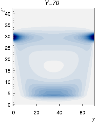
Figure 4: Transition from cigar–type evolution to tunneling–type evolution, figure from [87]

In such a situation the whole perturbative approach breaks down and the process is completely determined by the soft Pomeron.

The problem of diffusion in the BFKL Pomeron should always be kept in mind in phenomenological applications, in particular when the momentum scales of the external particles are only moderately large. So far the diffusion problem in the BFKL equation has only been studied in the LLA. It would be very interesting to see how the phenomenon is possibly modified in NLLA, and whether and at which energies the transition to a tunneling–like evolution occurs.

3.2 The Odderon in Perturbative QCD

In perturbative QCD the Odderon is a state of three interacting reggeized gluons exchanged in the $t$-channel. Let us first see how and why it is possible that an Odderon can be constructed as an object consisting of three gluons. Consider for simplicity a purely perturbative situation with small gluon fields $\mbox{\bf A}_{\mu}(x)=A^{a}_{\mu}(x)t^{a}$ where $t^{a}$ are the generators of the gauge group, and we consider the general case that the gauge group is $\mbox{SU}(N_{c})$. Under a charge conjugation transformation the behavior of the gluon fields is

$$\mbox{\bf A}_{\mu}(x)\longrightarrow-\mbox{\bf A}_{\mu}^{T}(x)\,.$$ (3.46)

It is quite obvious that there is only one possibility to form a color singlet state of two gluon operators, namely

$${\cal P}_{\mu\nu}(x,y) = \mbox{tr}\,(\mbox{\bf A}_{\mu}(x)\mbox{\bf A}_{\nu}(y))$$ (3.47)

$$= \frac{1}{2}\,\delta_{ab}A_{\mu}(x)A_{\nu}(y)\,.$$

From (3.46) we see that this state remains unchanged under charge conjugation and thus has $C=+1$. The exchange of two gluons in a color singlet state is then described by the free–field correlation function of the product of two such operators,

$$\langle\mbox{T}\,{\cal P}_{\mu^{\prime}\nu^{\prime}}(x^{\prime},y^{\prime}){\cal P}_{\mu\nu}(x,y)\rangle\,,$$ (3.48)

This is what we have called the Green function of the Pomeron in eq. (3.43). The exchange carries $C=+1$ and can be associated with the Pomeron. In the case of three gluons there are two ways of constructing a color singlet state. The first possibility is

$${\cal P}_{\mu\nu\rho}(x,y,z) = -i\,\mbox{tr}\,([\mbox{\bf A}_{\mu}(x),\mbox{\bf A}_{\nu}(y)]\mbox{\bf A}_{\rho}(z))$$ (3.49)

$$= \frac{1}{2}\,f_{abc}A^{a}_{\mu}(x)A^{b}_{\nu}(y)A^{c}_{\rho}(z)$$

with the structure constants $f_{abc}$ defined via the Lie algebra of $\mbox{SU}(N_{c})$

$$[t^{a},t^{b}]=if_{abc}t^{c}\,.$$ (3.50)

The $f_{abc}$ are totally antisymmetric, and one finds that also the operator ${\cal P}_{\mu\nu\rho}(x,y,z)$ is even under charge conjugation. Hence the corresponding exchange of three gluons has $C=+1$. (For a discussion of this exchange see the last paragraphs of sections 3.2.1 and 4.1.) The other possibility to form a color singlet state out of three gluon operators is

$${\cal O}_{\mu\nu\rho}(x,y,z) = \mbox{tr}\,(\{\mbox{\bf A}_{\mu}(x),\mbox{\bf A}_{\nu}(y)\}\mbox{\bf A}_{\rho}(z))$$ (3.51)

$$= \frac{1}{2}\,d_{abc}A^{a}_{\mu}(x)A^{b}_{\nu}(y)A^{c}_{\rho}(z)\,,$$

with the totally symmetric tensors

$$d_{abc}=2\,[\mbox{tr}(t^{a}t^{b}t^{c})+\mbox{tr}(t^{c}t^{b}t^{a})]\,.$$ (3.52)

Now one finds from (3.46) that this state is odd under charge conjugation, and the corresponding exchange carries $C=-1$. It can hence be associated with an Odderon. The crucial point is that the existence of the symmetric tensor $d_{abc}$ requires that the gauge group has a rank higher than one. This is the case for $\mbox{SU}(N_{c})$ as soon as $N_{c}\geq 3$, and hence the operator corresponding to the Odderon exists in QCD. In an $\mbox{SU}(2)$ gauge theory, however, it would not be possible to construct an operator corresponding to (3.51) since there the analogue of the tensor (3.52) vanishes, such that the antisymmetric $\epsilon_{ijk}$ is the only tensor that can be constructed of three generators of $\mbox{SU}(2)$.

Note that in the argument above we only made use of very general properties of the gluon fields, namely their behavior under a charge conjugation (3.46). This behavior will also hold for large fields $A$, and the argument should therefore also apply to nonperturbative situations. However, here the interpretation of the operator constructed from nonperturbative gluon fields might be ambiguous without specifying a nonperturbative framework for their exact definition and use.

Obviously, the above argument works for three elementary and non–interacting gluons. Accordingly, the use of a simple three–gluon exchange model satisfies the requirements for an Odderon. But the exchange of three non–interacting gluons leads to an Odderon intercept of exactly one, and it corresponds to a pole in the complex angular momentum plane. In the case of the BFKL Pomeron we have seen that resummation can lead to a quite different energy behavior and can hence have very significant effects. It is therefore obviously desirable to study resummation also in the case of the Odderon.

3.2.1 The Bartels-Kwieciński-Praszałowicz Equation

The resummation of large logarithms of the energy has for the Odderon been performed by Bartels [4], Jaroszewicz [5], and Kwieciński and Praszałowicz [6]. The corresponding equation is known as the Bartels–Kwieciński–Praszałowicz (BKP) equation.

The conceptual basis is again perturbative high energy factorization which separates the dynamics in transverse space from the longitudinal degrees of freedom. The amplitude is given as a convolution of the Odderon as a three–gluon compound state with the impact factors coupling it to the external particles. Diagrammatically this is shown in figure 5.

Figure 5: Factorization of the perturbative Odderon amplitude in the high energy limit

The corresponding equation will be given in eq. (4.2) further below when we turn to phenomenological applications. Here we will first concentrate on the amplitude $\phi_{\mbox{\scriptsize{\rm\kern 1.68004pt\vrule width=0.14003pt,height=4.37012pt,depth=-0.1507pt\kern-1.81996ptO}}}$ describing the Odderon exchanged between the scattering particles.

The BKP equation resums terms of the order $\alpha_{s}(\alpha_{s}\log s)^{n}$ with arbitrary $n$ in which three gluons in a $C=-1$ state are exchanged in the $t$-channel. It is in many respects very similar to the BFKL equation. It is an integral equation for the Green function of three reggeized gluons in the $t$-channel. It acts in two–dimensional transverse space and describes the pairwise interaction of the three gluons. As in the case of the BFKL equation we again consider partial wave amplitudes which are functions of the complex angular momentum $\omega$. (This dependence will always be understood but not written out explicitly.) The energy dependence of the amplitude at high energies can then be inferred from the singularities in the $\omega$-plane.

Let $\phi_{\mbox{\scriptsize{\rm\kern 1.68004pt\vrule width=0.14003pt,height=4.37012pt,depth=-0.1507pt\kern-1.81996ptO}}}({\bf k}_{1},{\bf k}_{2},{\bf k}_{3};{\bf k}^{\prime}_{1},{\bf k}^{\prime}_{2},{\bf k}^{\prime}_{3})$ be the amplitude for the scattering of three reggeized gluons with momenta ${\bf k}^{\prime}_{1}$, ${\bf k}^{\prime}_{2}$, ${\bf k}^{\prime}_{3}$ to three reggeized gluons with momenta ${\bf k}_{1}$, ${\bf k}_{2}$, ${\bf k}_{3}$. We again denote the transverse momentum transferred in the $t$-channel by ${\bf q}$, such that we have $\sum_{i=1}^{3}{\bf k}^{\prime}_{i}=\sum_{i=1}^{3}{\bf k}_{i}={\bf q}$. For brevity we will sometimes suppress the arguments ${\bf k}^{\prime}_{1},{\bf k}^{\prime}_{2},{\bf k}^{\prime}_{3}$ of the amplitude $\phi_{\mbox{\scriptsize{\rm\kern 1.68004pt\vrule width=0.14003pt,height=4.37012pt,depth=-0.1507pt\kern-1.81996ptO}}}$ in our notation. The amplitude $\phi_{\mbox{\scriptsize{\rm\kern 1.68004pt\vrule width=0.14003pt,height=4.37012pt,depth=-0.1507pt\kern-1.81996ptO}}}$ carries color labels $a_{1}$, $a_{2}$, $a_{3}$ for the three outgoing gluons. As we will see momentarily we do not need a second set of color labels for the incoming gluons.

We now give the BKP equation in momentum space in a form which can be easily generalized to the case of more than three gluons in the $t$-channel. That case will be discussed in more detail in section 3.3. Further below we will see that the BKP equation can be written in simpler notation in impact parameter space. In momentum space it is convenient to use the amputated amplitude $f_{\mbox{\scriptsize{\rm\kern 1.68004pt\vrule width=0.14003pt,height=4.37012pt,depth=-0.1507pt\kern-1.81996ptO}}}$ defined as

$$f_{\mbox{\scriptsize{\rm\kern 1.68004pt\vrule width=0.14003pt,height=4.37012pt,depth=-0.1507pt\kern-1.81996ptO}}}({\bf k}_{1},{\bf k}_{2},{\bf k}_{3})={\bf k}_{1}^{2}{\bf k}_{2}^{2}{\bf k}_{3}^{2}\,\phi_{\mbox{\scriptsize{\rm\kern 1.68004pt\vrule width=0.14003pt,height=4.37012pt,depth=-0.1507pt\kern-1.81996ptO}}}({\bf k}_{1},{\bf k}_{2},{\bf k}_{3})\,.$$ (3.53)

The BKP equation for $f_{\mbox{\scriptsize{\rm\kern 1.68004pt\vrule width=0.14003pt,height=4.37012pt,depth=-0.1507pt\kern-1.81996ptO}}}$ then reads

$$\left(\omega-\sum_{i=1}^{3}\beta({\bf k}_{i}^{2})\right)f_{\mbox{\scriptsize{\rm\kern 1.68004pt\vrule width=0.14003pt,height=4.37012pt,depth=-0.1507pt\kern-1.81996ptO}}}^{a_{1}a_{2}a_{3}}({\bf k}_{1},{\bf k}_{2},{\bf k}_{3}) = f_{\mbox{\scriptsize{\rm\kern 1.68004pt\vrule width=0.14003pt,height=4.37012pt,depth=-0.1507pt\kern-1.81996ptO}}}^{(0)\,a_{1}a_{2}a_{3}}({\bf k}_{1},{\bf k}_{2},{\bf k}_{3})$$

$$+\sum K^{\{b\}\rightarrow\{a\}}_{2\rightarrow 2}\otimes f_{\mbox{\scriptsize{\rm\kern 1.68004pt\vrule width=0.14003pt,height=4.37012pt,depth=-0.1507pt\kern-1.81996ptO}}}^{b_{1}b_{2}b_{3}}({\bf k}_{1},{\bf k}_{2},{\bf k}_{3})\,.$$

The function $\beta$ corresponds to the Regge trajectory of the gluon and is given explicitly in (3.12). We choose the inhomogeneous term $f_{\mbox{\scriptsize{\rm\kern 1.68004pt\vrule width=0.14003pt,height=4.37012pt,depth=-0.1507pt\kern-1.81996ptO}}}^{(0)}$ as

$$f_{\mbox{\scriptsize{\rm\kern 1.68004pt\vrule width=0.14003pt,height=4.37012pt,depth=-0.1507pt\kern-1.81996ptO}}}^{(0)\,a_{1}a_{2}a_{3}}({\bf k}_{1},{\bf k}_{2},{\bf k}_{3})=d_{a_{1}a_{2}a_{3}}\delta({\bf k}^{\prime}_{1}-{\bf k}_{1})\delta({\bf k}^{\prime}_{2}-{\bf k}_{2})\delta({\bf k}^{\prime}_{3}-{\bf k}_{3})$$ (3.55)

such that the lowest order term $\phi_{\mbox{\scriptsize{\rm\kern 1.68004pt\vrule width=0.14003pt,height=4.37012pt,depth=-0.1507pt\kern-1.81996ptO}}}^{(0)}$ of the Odderon amplitude $\phi_{\mbox{\scriptsize{\rm\kern 1.68004pt\vrule width=0.14003pt,height=4.37012pt,depth=-0.1507pt\kern-1.81996ptO}}}$ describes the free propagation of three gluons,

$$\phi_{\mbox{\scriptsize{\rm\kern 1.68004pt\vrule width=0.14003pt,height=4.37012pt,depth=-0.1507pt\kern-1.81996ptO}}}^{(0)\,a_{1}a_{2}a_{3}}({\bf k}_{1},{\bf k}_{2},{\bf k}_{3};{\bf k}^{\prime}_{1},{\bf k}^{\prime}_{2},{\bf k}^{\prime}_{3})=d_{a_{1}a_{2}a_{3}}\prod_{i=1}^{3}\frac{1}{{\bf k}_{i}^{2}}\,\delta({\bf k}^{\prime}_{i}-{\bf k}_{i})\,.$$ (3.56)

Here we have already specified the color tensor for the Odderon state. As discussed in the previous section the three gluons in the Odderon are in a symmetric color singlet state, hence the color tensor for the inhomogeneous term is $d_{a_{1}a_{2}a_{3}}$, and the same is true for the full amplitude,

$$\phi_{\mbox{\scriptsize{\rm\kern 1.68004pt\vrule width=0.14003pt,height=4.37012pt,depth=-0.1507pt\kern-1.81996ptO}}}^{a_{1}a_{2}a_{3}}({\bf k}_{1},{\bf k}_{2},{\bf k}_{3})=d_{a_{1}a_{2}a_{3}}\phi_{\mbox{\scriptsize{\rm\kern 1.68004pt\vrule width=0.14003pt,height=4.37012pt,depth=-0.1507pt\kern-1.81996ptO}}}({\bf k}_{1},{\bf k}_{2},{\bf k}_{3})\,,$$ (3.57)

and we use an analogous notation for the amputated amplitude $f_{\mbox{\scriptsize{\rm\kern 1.68004pt\vrule width=0.14003pt,height=4.37012pt,depth=-0.1507pt\kern-1.81996ptO}}}$. The color tensor remains (up to a constant factor) unchanged under the action of the kernel in the last term of the BKP equation to which we now turn. The interaction of the three gluons in the Odderon is pairwise, and the sum in the last term of the BKP equation (3.2.1) extends over all three pairs of gluons. We will give the kernel $K^{\{b\}\rightarrow\{a\}}_{2\rightarrow 2}$ explicitly for the case that the first two gluons interact, the other two combinations are readily obtained by a permutation of the labels. The superscript $\{b\}\rightarrow\{a\}$ of the kernel refers to the color part of the interaction of two reggeized gluons. The color structure of the kernel is

$$K^{\{b\}\rightarrow\{a\}}_{2\rightarrow 2}=f_{b_{1}a_{1}c}f_{ca_{2}b_{2}}\delta_{b_{3}a_{3}}K_{2\rightarrow 2}({\bf l}_{1},{\bf l}_{2};{\bf k}_{1},{\bf k}_{2})\,.$$ (3.58)

When contracted with the color tensor of the Odderon amplitude this yields a factor of $-N_{c}/2$,

$$f_{b_{1}a_{1}c}f_{ca_{2}b_{2}}\delta_{b_{3}a_{3}}d_{b_{1}b_{2}b_{3}}=-\frac{N_{c}}{2}\,d_{a_{1}a_{2}a_{3}}\,,$$ (3.59)

which is one half of the color factor occurring in the BFKL equation. As a side remark we note that the same factor $-N_{c}/2$ would be obtained if the three gluons were in an antisymmetric color state.

The momentum part $K_{2\rightarrow 2}({\bf l}_{1},{\bf l}_{2};{\bf k}_{1},{\bf k}_{2})$ of the kernel is given by

$$K_{2\rightarrow 2}({\bf l}_{1},{\bf l}_{2};{\bf k}_{1},{\bf k}_{2})=g^{2}\left[({\bf k}_{1}+{\bf k}_{2})^{2}-\frac{{\bf k}_{1}^{2}{\bf l}_{2}^{2}}{({\bf k}_{2}-{\bf l}_{2})^{2}}-\frac{{\bf k}_{2}^{2}{\bf l}_{1}^{2}}{({\bf k}_{1}-{\bf l}_{1})^{2}}\right]\,,$$ (3.60)

and is up to the color factor identical to the part of the BFKL kernel (3.1.1) corresponding to real gluon emission. The convolution $\otimes$ is the same as in the case of the BFKL kernel in (3.9), i. e. stands for a two–dimensional integration over the momentum ${\bf l}_{2}-{\bf l}_{1}$ with measure $1/(2\pi)^{3}$ and the propagators $1/({\bf l}_{1}^{2}{\bf l}_{2}^{2})$ of the two gluons involved in the interaction.

In the BKP equation (3.2.1) the terms containing the function $\beta$ correspond to virtual corrections, whereas the terms containing the kernel $K_{2\rightarrow 2}$ correspond to real gluon emission. They are not infrared finite separately, but the divergenes cancel between them. It turns out that the BKP equation can be written in terms of full BFKL kernels in which the cancellation of infrared divergences is already known. To see this we start from eq. (3.2.1) and bring the terms involving the function $\beta$ to the RHS. There is one of these terms for each reggeized gluon. There are three terms with kernels $K_{2\rightarrow 2}$ on the RHS, and the latter are up to the color factor identical to the real gluon emission part of the BFKL kernel. Each gluon is affected by the interaction described by two of these terms. We can hence distribute the functions $\beta$ in such a way that each kernel is associated with a term $\beta/2$ for each of the two gluons entering the kernel. The factor $1/2$ matches exactly the additional factor $1/2$ in the color factor of the kernel in the case of the Odderon. The interaction between two gluons is therefore given by $1/2$ times a full BFKL kernel (including virtual corrections) as given in (3.1.1).

The diagrammatic structure of the perturbative Odderon can be inferred by iteration of the BKP equation. That iteration yields ladder type diagrams in which the vertical lines represent reggeized gluons, and the ladder rungs represent BFKL kernels (now multiplied by $1/2$), see figure 6.

\begin{picture}(924.0,1284.0)(799.0,-793.0)\end{picture}

Figure 6: Ladder structure of the BKP Odderon

It is again very convenient to write the BKP equation in two–dimensional impact parameter space instead of transverse momentum space. We use the same notation as introduced in the previous section, in particular we have a set of holomorphic coordinates, denoted by $\rho$, and a set of antiholomorphic coordinates $\bar{\rho}$ for the three incoming and outgoing gluons. The partial wave amplitude $\phi_{\mbox{\scriptsize{\rm\kern 1.68004pt\vrule width=0.14003pt,height=4.37012pt,depth=-0.1507pt\kern-1.81996ptO}}}(\rho_{i},\bar{\rho}_{i};\rho_{j^{\prime}},\bar{\rho}_{j^{\prime}})$ in impact parameter is obtained via Fourier transformation in complete analogy to eq. (3.1.2). The coordinates $\rho_{i}$ ($i=1,2,3$) refer to the gluons with momenta ${\bf k}_{i}$, and analogously for the primed coordinates and momenta.

The BKP equation in impact parameter space becomes

$$\omega\phi_{\mbox{\scriptsize{\rm\kern 1.68004pt\vrule width=0.14003pt,height=4.37012pt,depth=-0.1507pt\kern-1.81996ptO}}}=\phi_{\mbox{\scriptsize{\rm\kern 1.68004pt\vrule width=0.14003pt,height=4.37012pt,depth=-0.1507pt\kern-1.81996ptO}}}^{(0)}+{\cal H}_{\mbox{\scriptsize{\rm\kern 1.68004pt\vrule width=0.14003pt,height=4.37012pt,depth=-0.1507pt\kern-1.81996ptO}}}\phi_{\mbox{\scriptsize{\rm\kern 1.68004pt\vrule width=0.14003pt,height=4.37012pt,depth=-0.1507pt\kern-1.81996ptO}}}\,.$$ (3.61)

The Hamiltonian ${\cal H}_{\mbox{\scriptsize{\rm\kern 1.68004pt\vrule width=0.14003pt,height=4.37012pt,depth=-0.1507pt\kern-1.81996ptO}}}$ can be split into two parts which act only on the holomorphic or antiholomorphic coordinates, respectively,

$${\cal H}_{\mbox{\scriptsize{\rm\kern 1.68004pt\vrule width=0.14003pt,height=4.37012pt,depth=-0.1507pt\kern-1.81996ptO}}}=\frac{\alpha_{s}N_{c}}{4\pi}\left(H_{\mbox{\scriptsize{\rm\kern 1.68004pt\vrule width=0.14003pt,height=4.37012pt,depth=-0.1507pt\kern-1.81996ptO}}}+\bar{H}_{\mbox{\scriptsize{\rm\kern 1.68004pt\vrule width=0.14003pt,height=4.37012pt,depth=-0.1507pt\kern-1.81996ptO}}}\right)\,,$$ (3.62)

and the two Hamiltonians $H_{\mbox{\scriptsize{\rm\kern 1.68004pt\vrule width=0.14003pt,height=4.37012pt,depth=-0.1507pt\kern-1.81996ptO}}}$ and $\bar{H}_{\mbox{\scriptsize{\rm\kern 1.68004pt\vrule width=0.14003pt,height=4.37012pt,depth=-0.1507pt\kern-1.81996ptO}}}$ commute with each other, $[H_{\mbox{\scriptsize{\rm\kern 1.68004pt\vrule width=0.14003pt,height=4.37012pt,depth=-0.1507pt\kern-1.81996ptO}}},\bar{H}_{\mbox{\scriptsize{\rm\kern 1.68004pt\vrule width=0.14003pt,height=4.37012pt,depth=-0.1507pt\kern-1.81996ptO}}}]=0$. The Hamiltonian hence exhibits holomorphic separability. The part acting on the holomorphic coordinates $\rho$ consists of three terms,

$$H_{\mbox{\scriptsize{\rm\kern 1.68004pt\vrule width=0.14003pt,height=4.37012pt,depth=-0.1507pt\kern-1.81996ptO}}}=H_{12}+H_{23}+H_{31}\,,$$ (3.63)

describing the pairwise interaction of the three reggeized gluons. The pairwise interaction is given by BFKL kernels up to a factor of $1/2$ which we have already taken into account in the prefactor in (3.62). Hence each of the three terms in $H_{\mbox{\scriptsize{\rm\kern 1.68004pt\vrule width=0.14003pt,height=4.37012pt,depth=-0.1507pt\kern-1.81996ptO}}}$ is given by the BFKL kernel (3.28) which can also be written as

$$H_{ij}=H_{\mbox{\scriptsize{\rm I\kern-1.75ptP}}}(\rho_{i},\rho_{j})=-\psi(-J_{ij})-\psi(1+J_{ij})+2\psi(1)\,.$$ (3.64)

The operator $J_{ij}$ is defined as an operator solution of the equation

$$J_{ij}(1+J_{ij})=L_{ij}=-(\rho_{i}-\rho_{j})^{2}\partial_{i}\partial_{j}\,.$$ (3.65)

Analogous relations hold for the part $\bar{H}_{\mbox{\scriptsize{\rm\kern 1.68004pt\vrule width=0.14003pt,height=4.37012pt,depth=-0.1507pt\kern-1.81996ptO}}}$ of the Hamiltionian that acts on the antiholomorphic coordinates.

In analogy to the case of the BFKL equation a formal solution of the BKP equation (3.61) is obtained via

$$\phi_{\mbox{\scriptsize{\rm\kern 1.68004pt\vrule width=0.14003pt,height=4.37012pt,depth=-0.1507pt\kern-1.81996ptO}}}=\frac{1}{\omega-{\cal H}_{\mbox{\scriptsize{\rm\kern 1.68004pt\vrule width=0.14003pt,height=4.37012pt,depth=-0.1507pt\kern-1.81996ptO}}}}\,\phi_{\mbox{\scriptsize{\rm\kern 1.68004pt\vrule width=0.14003pt,height=4.37012pt,depth=-0.1507pt\kern-1.81996ptO}}}^{(0)}\,.$$ (3.66)

The problem of finding the full solution $\phi_{\mbox{\scriptsize{\rm\kern 1.68004pt\vrule width=0.14003pt,height=4.37012pt,depth=-0.1507pt\kern-1.81996ptO}}}$ can therefore be formulated as the simpler problem of finding the eigenstates of the BKP Hamiltonian ${\cal H}_{\mbox{\scriptsize{\rm\kern 1.68004pt\vrule width=0.14003pt,height=4.37012pt,depth=-0.1507pt\kern-1.81996ptO}}}$,

$${\cal H}_{\mbox{\scriptsize{\rm\kern 1.68004pt\vrule width=0.14003pt,height=4.37012pt,depth=-0.1507pt\kern-1.81996ptO}}}\varphi_{\mbox{\scriptsize{\rm\kern 1.68004pt\vrule width=0.14003pt,height=4.37012pt,depth=-0.1507pt\kern-1.81996ptO}}}(\rho,\bar{\rho})=E\varphi_{\mbox{\scriptsize{\rm\kern 1.68004pt\vrule width=0.14003pt,height=4.37012pt,depth=-0.1507pt\kern-1.81996ptO}}}(\rho,\bar{\rho})\,,$$ (3.67)

and according to (3.66) the Odderon intercept is given by the largest eigenvalue $E$. Let us denote the set of quantum numbers of the three–gluon states satisfying this eigenvalue equation by $\{\alpha\}$ and the corresponding eigenvalues by $E_{\{\alpha\}}$. With a complete set of such eigenstates $\varphi_{{\mbox{\scriptsize{\rm\kern 1.68004pt\vrule width=0.14003pt,height=4.37012pt,depth=-0.1507pt\kern-1.81996ptO}}}\{\alpha\}}$ and a suitable scalar product on the corresponding Hilbert space the solution of the BKP equation can then be written as

$$\phi_{\mbox{\scriptsize{\rm\kern 1.68004pt\vrule width=0.14003pt,height=4.37012pt,depth=-0.1507pt\kern-1.81996ptO}}}=\sum_{\{\alpha\}}\frac{1}{\omega-E_{\{\alpha\}}}\left|\varphi_{{\mbox{\scriptsize{\rm\kern 1.68004pt\vrule width=0.14003pt,height=4.37012pt,depth=-0.1507pt\kern-1.81996ptO}}}\{\alpha\}}\right\rangle\left\langle\varphi_{{\mbox{\scriptsize{\rm\kern 1.68004pt\vrule width=0.14003pt,height=4.37012pt,depth=-0.1507pt\kern-1.81996ptO}}}\{\alpha\}}\right|\,\phi_{\mbox{\scriptsize{\rm\kern 1.68004pt\vrule width=0.14003pt,height=4.37012pt,depth=-0.1507pt\kern-1.81996ptO}}}^{(0)}\,,$$ (3.68)

with the summation symbol indicating the sum over discrete and the integration over continuous quantum numbers and parameters. In the case of the BFKL equation the quantum numbers of the eigenstates are given by the conformal weight $h$, see (3.34). In the case of the BKP equation the situation is more complicated. As we will discuss in detail in section 3.2.3 below the eigenstates of the BKP Hamiltonian carry an additional quantum number corresponding to the operator $q_{3}$. It turns out to be a non–trivial problem to identify those eigenstates of $q_{3}$ which are physically meaningful and should hence be included in the full solution (3.68). Although considerable progress has been made recently, a generally accepted answer to this question has yet to be found. We will discuss this problem in the following sections, see in particular section 3.2.7.

Due to the holomorphic separability of the BKP Hamiltonian ${\cal H}_{\mbox{\scriptsize{\rm\kern 1.68004pt\vrule width=0.14003pt,height=4.37012pt,depth=-0.1507pt\kern-1.81996ptO}}}$ the three–gluon eigenstates $\varphi_{\mbox{\scriptsize{\rm\kern 1.68004pt\vrule width=0.14003pt,height=4.37012pt,depth=-0.1507pt\kern-1.81996ptO}}}$ can be factorized into a product of functions depending only on holomorphic or antiholomorphic coordinates,

$$\varphi_{\mbox{\scriptsize{\rm\kern 1.68004pt\vrule width=0.14003pt,height=4.37012pt,depth=-0.1507pt\kern-1.81996ptO}}}(\rho,\bar{\rho})=\varphi(\rho)\bar{\varphi}(\bar{\rho})\,.$$ (3.69)

The Schrödinger equation (3.67) can hence be replaced by two separate equations for $\varphi$ and $\bar{\varphi}$,

$$H_{\mbox{\scriptsize{\rm\kern 1.68004pt\vrule width=0.14003pt,height=4.37012pt,depth=-0.1507pt\kern-1.81996ptO}}}\varphi(\rho) = \epsilon\varphi(\rho)$$ (3.70)

$$\bar{H}_{\mbox{\scriptsize{\rm\kern 1.68004pt\vrule width=0.14003pt,height=4.37012pt,depth=-0.1507pt\kern-1.81996ptO}}}\bar{\varphi}(\bar{\rho}) = \bar{\epsilon}\bar{\varphi}(\bar{\rho})\,,$$ (3.71)

and we have

$$E=\frac{\alpha_{s}N_{c}}{4\pi}(\epsilon+\bar{\epsilon})\,.$$ (3.72)

Thereby the description of the perturbative Odderon has been reduced to the problem of solving two (identical) eigenvalue problems for the holomorphic and antiholomorphic Hamiltonians $H_{\mbox{\scriptsize{\rm\kern 1.68004pt\vrule width=0.14003pt,height=4.37012pt,depth=-0.1507pt\kern-1.81996ptO}}}$ and $\bar{H}_{\mbox{\scriptsize{\rm\kern 1.68004pt\vrule width=0.14003pt,height=4.37012pt,depth=-0.1507pt\kern-1.81996ptO}}}$.

Concluding this section a remark is in order concerning the exchange of three gluons in the $t$-channel carrying positive charge parity $C=+1$. We have already seen the corresponding three–gluon operator in (3.49). Because of its quantum numbers this state can be considered a Pomeron state. It has not yet been studied in much detail so far, but we expect it to be quite interesting and important. In contrast to the Odderon, the three gluons are in an antisymmetric color state given by the color tensor $f_{abc}$ of su(3). In perturbation theory this state is described by a BKP equation in the $C=+1$ sector. The color factors in the kernels of the BKP equation are the same for symmetric and antisymmetric octet states, and therefore the resulting BKP equation for the momentum part of the $C=+1$ three–gluon state is identical to the one for the Odderon, but the solutions have different symmetry properties. The energy levels of the corresponding Hamiltonian are therefore not identical to those of the Odderon, although some degeneracies are not excluded. The contribution of the three–gluon Pomeron or Odderon state to scattering cross sections strongly depends on the particular scattering process even in cases where both exchanges are present. The latter is the case when the initial and final states are not eigenstates of $C$-parity. In general the impact factors describing the coupling to the external particles project out different contributions in the $C=+1$ and $C=-1$ channels. For further discussion of the $C=+1$ three–gluon exchange we refer the reader to section 3.3.2 and to the last paragraph of section 4.1.

3.2.2 Conformal Invariance of the BKP Equation

As we have just seen the BKP Hamiltonian can be decomposed into BFKL Hamiltonians. The latter are invariant under conformal transformations in two–dimensional impact parameter space, and so is hence the BKP Hamiltonian. Technically speaking, the Hamiltonian ${\cal H}_{\mbox{\scriptsize{\rm\kern 1.68004pt\vrule width=0.14003pt,height=4.37012pt,depth=-0.1507pt\kern-1.81996ptO}}}$ commutes with the operator

$$q_{2}=L^{2}=L_{12}^{2}+L_{23}^{2}+L_{31}^{2}$$ (3.73)

with $L_{ij}$ defined in (3.65) and an operator $\bar{q}_{2}$ defined similarly in the antiholomorphic sector. This holds separately for the holomorphic part of ${\cal H}_{\mbox{\scriptsize{\rm\kern 1.68004pt\vrule width=0.14003pt,height=4.37012pt,depth=-0.1507pt\kern-1.81996ptO}}}$,

$$[q_{2},H_{\mbox{\scriptsize{\rm\kern 1.68004pt\vrule width=0.14003pt,height=4.37012pt,depth=-0.1507pt\kern-1.81996ptO}}}]=[\bar{q}_{2},H_{\mbox{\scriptsize{\rm\kern 1.68004pt\vrule width=0.14003pt,height=4.37012pt,depth=-0.1507pt\kern-1.81996ptO}}}]=0\,,$$ (3.74)

and its antiholomorphic counterpart $\bar{H}_{\mbox{\scriptsize{\rm\kern 1.68004pt\vrule width=0.14003pt,height=4.37012pt,depth=-0.1507pt\kern-1.81996ptO}}}$. The operator $q_{2}$ is the quadratic Casimir operator of $\mbox{SL}(2,{\rm\kern 2.40005pt\vrule width=0.20004pt,height=6.02773pt,depth=-0.21529pt\kern-2.59995ptC})$ on the space of three–gluon states, and according to the group theory of $\mbox{SL}(2,{\rm\kern 2.40005pt\vrule width=0.20004pt,height=6.02773pt,depth=-0.21529pt\kern-2.59995ptC})$ its eigenvalues can take the values

$$q_{2}=-h(h-1)\,,$$ (3.75)

where $h$ is the conformal weight of the corresponding eigenstate. The conformal weight is again quantized as $h=(1+n)/2+i\nu$ with $n\in{\rm\kern 2.59995pt\vrule width=0.20004pt,height=2.15277pt,depth=0.0pt\kern 0.39993pt\vrule width=0.20004pt,height=6.32915pt,depth=-4.30554pt\kern-3.39996ptZ}$ and $\nu\in{\rm I\kern-2.10007ptR}$.

Conformal invariance places very strong constraints on the eigenfunctions of the Hamiltonian ${\cal H}_{\mbox{\scriptsize{\rm\kern 1.68004pt\vrule width=0.14003pt,height=4.37012pt,depth=-0.1507pt\kern-1.81996ptO}}}$. We recall that in the case of the BFKL equation the eigenfunctions with given conformal weight are fixed up to a normalization, see (3.34). In the case of the three–gluon states of the Odderon there is slightly more freedom in the dependence of the eigenstates on the coordinates. Here the eigenfunctions of ${\cal H}_{\mbox{\scriptsize{\rm\kern 1.68004pt\vrule width=0.14003pt,height=4.37012pt,depth=-0.1507pt\kern-1.81996ptO}}}$ parametrized by conformal weights $h$ and $\bar{h}=1-h^{*}$ have the general form [88, 89, 90]

$$\varphi^{(h,\bar{h})}_{\mbox{\scriptsize{\rm\kern 1.68004pt\vrule width=0.14003pt,height=4.37012pt,depth=-0.1507pt\kern-1.81996ptO}}}(\rho,\bar{\rho};\rho_{0})=\left(\frac{\rho_{12}\rho_{13}\rho_{23}}{\rho_{10}^{2}\rho_{20}^{2}\rho_{30}^{2}}\right)^{h/3}\left(\frac{\bar{\rho}_{12}\bar{\rho}_{13}\bar{\rho}_{23}}{\bar{\rho}_{10}^{2}\bar{\rho}_{20}^{2}\bar{\rho}_{30}^{2}}\right)^{\bar{h}/3}\phi^{(h,\bar{h})}(z,\bar{z})\,,$$ (3.76)

in which the dependence on the coordinates is fixed up to a function of the anharmonic ratio

$$z=\frac{\rho_{12}\rho_{30}}{\rho_{13}\rho_{20}}$$ (3.77)

and the similarly defined ratio $\bar{z}$. As in the case of the BFKL equation the coordinate $\rho_{0}$ is an additional parameter of the eigenstates. Due to the holomorphic separability of the Odderon Hamiltonian ${\cal H}_{\mbox{\scriptsize{\rm\kern 1.68004pt\vrule width=0.14003pt,height=4.37012pt,depth=-0.1507pt\kern-1.81996ptO}}}$ the function $\phi^{(h,\bar{h})}(z,\bar{z})$ in (3.76) can be further factorized as

$$\phi^{(h,\bar{h})}(z,\bar{z})=\phi^{(h)}(z)\,\bar{\phi}^{(\bar{h})}(\bar{z})\,.$$ (3.78)

The function $\phi^{(h,\bar{h})}(z,\bar{z})$ is not arbitrary but has to satisfy constraints related to the operator $q_{3}$ to which we turn in the next section. Assuming a non–singular behavior of $\phi^{(h,\bar{h})}(z,\bar{z})$ one can deduce from (3.76) that the Odderon state $\varphi^{(h,\bar{h})}_{\mbox{\scriptsize{\rm\kern 1.68004pt\vrule width=0.14003pt,height=4.37012pt,depth=-0.1507pt\kern-1.81996ptO}}}$ vanishes if two of the gluon coordinates $\rho_{i}$ coincide. This is in fact true for the case that the eigenvalue of the operator $q_{3}$ does not vanish. In the case that $q_{3}=0$, however, the function $\varphi^{(h,\bar{h})}_{\mbox{\scriptsize{\rm\kern 1.68004pt\vrule width=0.14003pt,height=4.37012pt,depth=-0.1507pt\kern-1.81996ptO}}}$ can be highly singular and can even be a distribution rather than a function. We will discuss a solution of that type in section 3.2.6.

The eigenfunctions $\varphi^{(h,\bar{h})}_{\mbox{\scriptsize{\rm\kern 1.68004pt\vrule width=0.14003pt,height=4.37012pt,depth=-0.1507pt\kern-1.81996ptO}}}$ can be interpreted as four–point functions of a conformal field theory. This can be illustrated pictorially as

$$\varphi^{(h,\bar{h})}_{\mbox{\scriptsize{\rm\kern 1.68004pt\vrule width=0.14003pt,height=4.37012pt,depth=-0.1507pt\kern-1.81996ptO}}}\>\>\>=\>\>\>\hbox{\raise-29.65955pt\hbox{\begin{picture}(0.0,0.0)\includegraphics{oddioperator.pstex}\end{picture}\begin{picture}(540.0,1033.0)(1216.0,-704.0)\put(1576.0,164.0){\makebox(0.0,0.0)[lb]{\smash{${\rm\kern 2.40005pt\vrule width=0.20004pt,height=6.24301pt,depth=-0.21529pt\kern-2.59995ptO}$}}} \put(1756.0,-646.0){\makebox(0.0,0.0)[lb]{\smash{$\phi_{3}$}}} \put(1216.0,-646.0){\makebox(0.0,0.0)[lb]{\smash{$\phi_{1}$}}} \put(1486.0,-646.0){\makebox(0.0,0.0)[lb]{\smash{$\phi_{2}$}}} \end{picture} }}\>\>\>=\>\>\>\langle\phi_{1}\,\phi_{2}\,\phi_{3}\,{\cal O}^{\mbox{\scriptsize{\rm\kern 1.68004pt\vrule width=0.14003pt,height=4.37012pt,depth=-0.1507pt\kern-1.81996ptO}}}\rangle$$ (3.79)

where $\rho_{0}$ can be identified with the coordinate of the three–gluon compound state corresponding to the operator ${\cal O}^{\mbox{\scriptsize{\rm\kern 1.68004pt\vrule width=0.14003pt,height=4.37012pt,depth=-0.1507pt\kern-1.81996ptO}}}$. The full Green function $\phi_{\mbox{\scriptsize{\rm\kern 1.68004pt\vrule width=0.14003pt,height=4.37012pt,depth=-0.1507pt\kern-1.81996ptO}}}$ of the Odderon can then be understood as a six–point function, pictorially

$$\phi_{\mbox{\scriptsize{\rm\kern 1.68004pt\vrule width=0.14003pt,height=4.37012pt,depth=-0.1507pt\kern-1.81996ptO}}}\>\>\>=\>\>\>\hbox{\raise-39.3341pt\hbox{\begin{picture}(0.0,0.0)\includegraphics{oddigreen.pstex}\end{picture}\begin{picture}(540.0,1339.0)(1216.0,-704.0)\put(1486.0,479.0){\makebox(0.0,0.0)[lb]{\smash{$\phi_{2}$}}} \put(1756.0,-646.0){\makebox(0.0,0.0)[lb]{\smash{$\phi_{3^{\prime}}$}}} \put(1216.0,-646.0){\makebox(0.0,0.0)[lb]{\smash{$\phi_{1^{\prime}}$}}} \put(1216.0,479.0){\makebox(0.0,0.0)[lb]{\smash{$\phi_{1}$}}} \put(1756.0,479.0){\makebox(0.0,0.0)[lb]{\smash{$\phi_{3}$}}} \put(1486.0,-646.0){\makebox(0.0,0.0)[lb]{\smash{$\phi_{2^{\prime}}$}}} \end{picture} }}\>\>\>=\>\>\>\langle\,\phi_{1}\,\phi_{2}\,\phi_{3}\,\phi_{1^{\prime}}\,\phi_{2^{\prime}}\,\phi_{3^{\prime}}\,\rangle\,.$$ (3.80)

This can also be interpreted as a diagrammatic form of eq. (3.68).

3.2.3 The Odderon as an Integrable Model

Remarkably, the Hamiltonian ${\cal H}_{\mbox{\scriptsize{\rm\kern 1.68004pt\vrule width=0.14003pt,height=4.37012pt,depth=-0.1507pt\kern-1.81996ptO}}}$ associated with the perturbative Odderon possesses an additional hidden symmetry and turns out to be equivalent to a completely integrable model. The discovery of this equivalence was an important breakthrough in the understanding of the perturbative Odderon. In fact most of the recent results on the Odderon rest on its integrability. Most importantly, the development triggered by that discovery has lead to the precise determination of the perturbative Odderon intercept.

We have already seen in the previous section that the Odderon Hamiltonian ${\cal H}_{\mbox{\scriptsize{\rm\kern 1.68004pt\vrule width=0.14003pt,height=4.37012pt,depth=-0.1507pt\kern-1.81996ptO}}}$ possesses an integral of motion $q_{2}$ related to the conformal invariance in impact parameter space. In addition, the total transverse momentum of the three reggeized gluons,

$$P=-i\partial_{1}-i\partial_{2}-i\partial_{3}\,,$$ (3.81)

is a conserved quantity in the $t$-channel evolution, i. e. under the action of the Odderon Hamiltonian, $[P,{\cal H}_{\mbox{\scriptsize{\rm\kern 1.68004pt\vrule width=0.14003pt,height=4.37012pt,depth=-0.1507pt\kern-1.81996ptO}}}]=0$. With $q_{2}$ and $P$ we have two conserved charges in the holomorphic sector, and also the corresponding operators $\bar{q}_{2}$ and $\bar{P}$ in the antiholomorphic sector are conserved. For the complete integrability of the problem one more integral of motion and its antiholomorphic counterpart are required. It was discovered in [91] that the Odderon indeed has an additional conserved charge associated with the operator $q_{3}$ defined as

$$q_{3}=-i\rho_{12}\rho_{23}\rho_{31}\partial_{1}\partial_{2}\partial_{3}\,,$$ (3.82)

and a similarly defined operator $\bar{q}_{3}$ in the antiholomorphic sector. These operators commute with the Hamiltonian $H_{\mbox{\scriptsize{\rm\kern 1.68004pt\vrule width=0.14003pt,height=4.37012pt,depth=-0.1507pt\kern-1.81996ptO}}}$,

$$[q_{3},H_{\mbox{\scriptsize{\rm\kern 1.68004pt\vrule width=0.14003pt,height=4.37012pt,depth=-0.1507pt\kern-1.81996ptO}}}]=[\bar{q}_{3},H_{\mbox{\scriptsize{\rm\kern 1.68004pt\vrule width=0.14003pt,height=4.37012pt,depth=-0.1507pt\kern-1.81996ptO}}}]=0\,,$$ (3.83)

as well as with $\bar{H}_{\mbox{\scriptsize{\rm\kern 1.68004pt\vrule width=0.14003pt,height=4.37012pt,depth=-0.1507pt\kern-1.81996ptO}}}$ and hence with the full Odderon Hamiltonian ${\cal H}_{\mbox{\scriptsize{\rm\kern 1.68004pt\vrule width=0.14003pt,height=4.37012pt,depth=-0.1507pt\kern-1.81996ptO}}}$.

In [92] (see also [93]) it was subsequently shown that the origin of the conserved charge is the equivalence of the perturbative Odderon with the XXX Heisenberg model of spin $s=0$, consisting of a closed spin chain containing three sites. It was found that this equivalence actually goes far beyond the Odderon itself. It extends to the large-$N_{c}$ limit of the general case of an arbitrary but fixed number of reggeized gluons in the generalized leading logarithmic approximation. Such a system is described by a straightforward generalization of the BKP equation for the Odderon to a larger number of reggeized gluons. That system will be the subject of section 3.3.1, where we will also give a detailed account of the equivalence with the XXX Heisenberg model. It is important to note that for an arbitrary number of reggeized gluons the equivalence holds only in the large-$N_{c}$ limit. But in the case of the Odderon, i. e. for three reggeized gluons, the equivalence is exact already for finite $N_{c}$ and does not require any further assumptions.

The complete integrability implies that the Odderon Hamiltonian is a function of the conserved charges $P$, $q_{2}$, $q_{3}$ and their antiholomorphic counterparts. As a consequence of the Möbius invariance the Hamiltonian does not depend on the total momentum $P$ of the three reggeized gluons, and we have for example for the holomorphic sector

$$H_{\mbox{\scriptsize{\rm\kern 1.68004pt\vrule width=0.14003pt,height=4.37012pt,depth=-0.1507pt\kern-1.81996ptO}}}=H_{\mbox{\scriptsize{\rm\kern 1.68004pt\vrule width=0.14003pt,height=4.37012pt,depth=-0.1507pt\kern-1.81996ptO}}}(q_{2},q_{3})\,.$$ (3.84)

Hence the determination of the eigenvalues of the Hamiltonian is equivalent to the simultaneous diagonalization of the operators $P$, $q_{2}$, and $q_{3}$. The possible eigenvalues of the operator $q_{2}$ are fixed by the representation theory of the symmetry group $\mbox{SL}(2,{\rm\kern 2.40005pt\vrule width=0.20004pt,height=6.02773pt,depth=-0.21529pt\kern-2.59995ptC})$ as discussed above. Therefore the spectrum of the Odderon Hamiltonian can be found by calculating the spectrum of the operator $q_{3}$. We should add though that the dependence of the Hamiltonian $H_{\mbox{\scriptsize{\rm\kern 1.68004pt\vrule width=0.14003pt,height=4.37012pt,depth=-0.1507pt\kern-1.81996ptO}}}$ on the conserved charges is very complicated, and there is no simple explicit form of (3.84).

The quantization condition for the possible eigenvalues of the operator $q_{3}$ comes from the requirement that the Odderon wave function has to be single–valued. So far we have considered the holomorphic and antiholomorphic parts of the Odderon Hamiltonian separately. But the physical wave function of the Odderon must clearly be single–valued in the complete transverse impact parameter plane, i. e. for the physical region in which $\bar{\rho}=\rho^{*}$, and by this condition the holomorphic and the antiholomorphic sector are tied together. Two further requirements are the normalizability of the wave function and its Bose symmetry. It turns out that the latter two requirements are easily fulfilled, and it is the single–valuedness condition which is instrumental in finding the quantization condition for the conserved charge $q_{3}$.

Motivated by the complete integrability of the Odderon the use of a generalized Bethe ansatz was suggested for this problem in [92, 93]. That method is based on the Baxter $Q$-operator and the separation of variables in the Sklyanin representation of the wave function. It can be successfully applied also to the more general case of a state of a fixed number of reggeized gluons in the large-$N_{c}$ limit of the generalized leading logarithmic approximation, see section 3.3.1. Again we emphasize that in the case of the Odderon the method works also for finite $N_{c}$. The method relies on the existence of the Baxter $Q$-operator ${\bf Q}(\lambda)$. It depends on a complex spectral parameter $\lambda$, and commutes with itself for different values of the spectral parameter, $[{\bf Q}(\mu),{\bf Q}(\lambda)]=0$, as well as with the conserved charges, $[{\bf Q}(\lambda),q_{2}]=[{\bf Q}(\lambda),q_{3}]=0$. The eigenvalues $Q(\lambda)$ of the Baxter $Q$-operator satisfy the Baxter equation which in the case of the Odderon reads

$$(2\lambda^{3}+q_{2}\lambda+q_{3})Q(\lambda)=(\lambda+i)^{3}Q(\lambda+i)+(\lambda-i)^{3}Q(\lambda-i)\,,$$ (3.85)

where $q_{2}$ and $q_{3}$ here denote the eigenvalues of the corresponding operators. In addition to the Baxter equation there are two more conditions which the Baxter $Q$-operator has to fulfill: it is a meromorphic function with known pole structure, and it has to exhibit a known asymptotic behavior at infinity. Analogous conditions hold for the Baxter operator in the antiholomorphic sector. It can be shown that the Baxter equation (3.85) and the other two conditions fix the Baxter $Q$-operator uniquely, and consequently also determine the quantization of the conserved charges $q_{2}$ and $q_{3}$. For given eigenvalues $q_{2}$ and $q_{3}$ one can then obtain the eigenvalue $\epsilon$ of the Hamiltonian $H_{\mbox{\scriptsize{\rm\kern 1.68004pt\vrule width=0.14003pt,height=4.37012pt,depth=-0.1507pt\kern-1.81996ptO}}}$ via

$$\epsilon(q_{2},q_{3})=-6+i\frac{d}{d\lambda}\log\left.\frac{Q(\lambda-i)}{Q(\lambda+i)}\right|_{\lambda=0}\,,$$ (3.86)

and one can hence compute the intercept as well as the full spectrum of the Odderon from the eigenvalues of the Baxter operator. A useful way to deal with the Baxter equation is to write $Q(\lambda)$ in terms of a contour integral [92]

$$Q(\lambda)=\int_{C}\frac{dx}{2\pi i}\,x^{-i\lambda-1}(x-1)^{i\lambda-1}\tilde{Q}(x)\,,$$ (3.87)

with a closed path $C$ in the complex $x$-plane, after which the Baxter equation (3.85) is transformed into a third–order differential equation for $\tilde{Q}$. The condition on the asymptotic behavior of $Q$ mentioned above implies that $\tilde{Q}(x)\to x^{h-2}$ as $x\to\infty$.

The problem of the quantization condition for the conserved charge $q_{3}$ has been considered in a number of papers [93]–[109]. Of these the papers [93]–[96] deal with different aspects of the Baxter equation in the Bethe ansatz approach. In [102] the quantization condition was studied in a more direct approach. Here the single–valuedness condition for the wave function was discussed in the context of a further duality symmetry of the Odderon Hamiltonian to which we will turn in more detail in the next section. Also the investigation of the perturbative Odderon problem in the quasiclassical (WKB) approximation in [95, 96, 98, 99] was fruitful in several respects. Firstly, it has turned out that the exact spectra of the conserved charge $q_{3}$ and of the Odderon Hamiltonian ${\cal H}_{\mbox{\scriptsize{\rm\kern 1.68004pt\vrule width=0.14003pt,height=4.37012pt,depth=-0.1507pt\kern-1.81996ptO}}}$ are reproduced to surprising accuracy in that approximation [107, 109]. This renders the WKB approximation a very valuable tool in the study of the perturbative Odderon problem. Secondly, the WKB approximation has made it possible to establish that the perturbative Odderon bears interesting relations to the integrable structures found in Seiberg–Witten dynamics of ${\cal N}=2$ supersymmetric QCD [96] as well as to the dynamics of solitonic waves [98].

The intercept of the solutions with $q_{3}\neq 0$ was first found in [97] and [100]. In [97] an exact method was devised to solve the Baxter equation for arbitrary values of the conserved charges $q_{2}$ and $q_{3}$. This method uses a double contour integral representation of the eigenvalue of the Baxter operator in which the latter is written as the sum of two terms of the form (3.87). With suitably chosen contours this allows one to implement the cancellation of boundary terms arising from integration by parts. That cancellation is not possible in a single–contour integral representation due to the particular structure of the Riemann surface of the integrand. In this way it is possible to find a unique solution of the Baxter equation within the ansatz of the double–contour integration. A more direct approach was then used in [100] to construct the quantization condition for the conserved charge $q_{3}$ and to determine the corresponding eigenfunction of the Odderon Hamiltonian. That construction will be described in section 3.2.5 below. From the values for $q_{3}$ found by this construction it was then possible to compute the Odderon intercept via the method of [97] outlined above. In these studies it was assumed that the maximal eigenvalue of the Odderon Hamiltonian is obtained for the conformal weight $h=1/2$. Subsequent studies of the Odderon intercept for arbitrary conformal weights $h$ in [101, 105] have confirmed that assumption.

In [103, 108] and in [104, 106, 107] finally the full spectrum of the operator $q_{3}$ and of the Odderon Hamiltonian ${\cal H}_{\mbox{\scriptsize{\rm\kern 1.68004pt\vrule width=0.14003pt,height=4.37012pt,depth=-0.1507pt\kern-1.81996ptO}}}$ was computed using the method of the Baxter ${\bf Q}$-operator. The results for the spectrum were compared to the corresponding results in the WKB approximation in [109], and again a good agreement was found. There is, however, a fundamental difference between [108] and [106, 107] concerning the physical interpretation of the results which we will discuss momentarily.

A detailed account of all studies of the integrability properties of the Odderon mentioned above would clearly go beyond the scope of the present review. We therefore restrict ourselves to the description of the main results and of the presently open problems. In sections 3.2.5 and 3.2.6 we will discuss the explicitly known solutions of the BKP equation. The significance of these two solutions and the Odderon intercept will then be the subject of section 3.2.7. Concluding the present section we now discuss the possible eigenvalues of the operator $q_{3}$.

There exist eigenfunctions of the Hamiltonian $H_{\mbox{\scriptsize{\rm\kern 1.68004pt\vrule width=0.14003pt,height=4.37012pt,depth=-0.1507pt\kern-1.81996ptO}}}$ both for the quantum number $q_{3}=0$ as well as for $q_{3}\neq 0$. As we will see in detail below their properties are quite different. The solutions with $q_{3}=0$ (see section 3.2.6) require to extend the Hilbert space of the Odderon Hamiltonian such that also distributions and not only smooth functions are included. Such an extension appears very natural due to the phenomenon of reggeization. Although this extension needs further study the solutions with $q_{3}=0$ are generally accepted as physical solutions. The situation is more complicated in the case of solutions with $q_{3}\neq 0$. For this case the full spectrum of $q_{3}$ has been computed in [103, 108] and in [104, 106, 107]. The results of these two groups agree as far as purely imaginary values of $q_{3}$ are concerned. However, there is a disagreement concerning the case of general complex values of $q_{3}$ with nonvanishing real part. The authors of [108] find that the corresponding eigenfunctions of the Hamiltonian are unphysical, whereas in [107] it is argued that completeness of the eigenfunctions requires to include them. Clearly, further study is needed to clarify this important question. Note however that this disagreement does not affect the determination of the Odderon intercept because the state with the highest eigenvalue $E$ corresponds to a purely imaginary value of $q_{3}$.

3.2.4 Modular Invariance of the BKP Equation

A very interesting symmetry of the Odderon wave function was observed in [89] and further discussed in [110, 111]. Both the Hamiltonian $H_{\mbox{\scriptsize{\rm\kern 1.68004pt\vrule width=0.14003pt,height=4.37012pt,depth=-0.1507pt\kern-1.81996ptO}}}$ of the Odderon as well as the conserved charge $q_{3}$ are invariant under cyclic permutations of the gluon coordinates $\rho_{i}$. This invariance is a direct consequence of Bose symmetry for the three–gluon state. We should note here that the invariance under cyclic permutations of the gluon coordinates also applies to the more general case of $N$-gluon states in the large-$N_{c}$ limit of the GLLA. The situation is, however, slightly different for more than $3$ gluons since in that case the cyclic permutations together with the inversion of the order do not exhaust the complete permutation group as in the case of the Odderon.

Under the repeated cyclic permutation $\rho_{1}\to\rho_{2}\to\rho_{3}$ the anharmonic ratio $z$ transforms as

$$z\,\,\,\longrightarrow\,\,\,1-\frac{1}{z}\,\,\,\longrightarrow\,\,\,\frac{1}{1-z}\,,$$ (3.88)

and the analogous transformation property holds for $\bar{z}$ in the antiholomorphic sector. The invariance under this transformation is called modular invariance. As shown in [110, 111] the invariance under cyclic permutations of the gluon coordinates in fact allows one to relate the Odderon problem to the modular invariance in the theory of elliptic curves. It can be shown that as a result of modular invariance the function $\phi^{(h)}(z)$ in (3.78) depends on $z$ in a special way, namely it is a function of the ratio

$$\xi=\frac{i}{3\sqrt{3}}\,\frac{(z-2)(z+1)(2z-1)}{z(z-1)}$$ (3.89)

only, and a similar result holds for $\bar{\phi}^{(\bar{h})}(\bar{z})$. This property was later used in [101, 105] for constructing the quantization conditions for the conserved charge $q_{3}$. The invariance of the Odderon under cyclic permutations was also used in [112] for finding a new representation for the Odderon wave function. It classifies it according to a new quantum number triality $\lambda$ for which $\lambda^{3}=1$. In this way simultaneous eigenfunctions of $q_{2}$ and $q_{3}$ were constructed which possess definite triality. Also here the quantization condition for $q_{3}$ can be studied by making use of this decomposition. The new representation is also useful for calculating the eigenvalues of a wide class of operators.

There is an interesting consequence of the modular invariance of the Odderon for the spectrum of the operator $q_{3}$. The eigenvalues of $q_{3}$ found in [106, 107] have a lattice–like structure in the complex plane. (Note however that the physical significance of those eigenstates of $q_{3}$ with eigenvalues that are not purely imaginary is still unclear, see the discussion in sections 3.2.3 and 3.2.7.) The origin of that lattice–like structure becomes particularly transparent in the quasiclassical (WKB) approximation [109]. There it is shown that the modular invariance can be related to the properties of the Riemann surface defined by the spectral curve of the resulting integrable model. The same Riemann surface is also of central interest in the attempt to interpret the Odderon and higher $N$-gluon states in the GLLA in terms of string theory amplitudes [113].

Another interesting symmetry of the Odderon was discovered in [102]. It was found there that the conserved charges $q_{2}$ and $q_{3}$ and hence also the Odderon Hamiltonian $H_{\mbox{\scriptsize{\rm\kern 1.68004pt\vrule width=0.14003pt,height=4.37012pt,depth=-0.1507pt\kern-1.81996ptO}}}$ are invariant under a duality transformation which relates the coordinates to the corresponding derivative operators, i. e. to the momenta of the reggeized gluons. Specifically, the duality transformation is given by

$$\rho_{i-1,i}\longrightarrow i\partial_{i}\longrightarrow\rho_{i,i+1}$$ (3.90)

(with the cyclic identification $\rho_{4}=\rho_{1}$) and the simultaneous reversing of the order of the operator multiplication. If the duality transformation is performed twice one is led to the cyclic permutation of the gluon coordinates discussed above. The invariance under cyclic permutations and the resulting modular invariance is hence closely related also to the invariance under the duality transformation.

This duality symmetry has an immediate consequence for the Odderon wave function. In the next section we will discuss the form of the wave function for the class of solutions for which $q_{3}\neq 0$. In the representation that we introduce there the wave function is determined by three parameters. It turns out that in this representation the condition resulting from the invariance under the duality transformation has a particularly simple form. It says that the ratio of two of the wave function parameters must equal the modulus of the quantized eigenvalue of the operator $q_{3}$ for the corresponding solution. The invariance under the duality transformation is hence closely related also to the quantization condition for the operator $q_{3}$.

Let us finally note that the invariance under the duality transformation holds also for the more general case of a fixed number $N$ of reggeized gluons in the large-$N_{c}$ limit of the GLLA. Interestingly, the above duality transformation coincides with a supersymmetric translation in the limit $N\to\infty$. It has been suggested in [102] that this indicates a close relationship of the integrability of the $N$-gluon states in the large-$N_{c}$ limit of the GLLA with supersymmetric field theories and superstring theories.

3.2.5 The Janik-Wosiek Solution

Exact eigenfunctions of the operator $q_{3}$ and of the BKP Odderon Hamiltonian have been found by Janik and Wosiek in [100], and we will call them JW solutions. These eigenfunctions have quantum numbers $q_{3}\neq 0$. The advantage of the method of [100] is that it not only allows one to find the quantization of the eigenvalues of $q_{3}$ and the Odderon intercept but also to obtain the Odderon wave function in explicit form.

Since the operators $q_{2}$ and $q_{3}$ commute one can find a set of simultaneous eigenfunctions for these operators. We have seen in section 3.2.2 that the eigenfunctions of the Odderon Hamiltonian can be written in conformally invariant form diagonalizing $q_{2}$, see (3.76) together with (3.78). One can use that form of the eigenfunctions and find the quantization condition of the operator $q_{3}$. For fixed $q_{2}$ the eigenvalue equation for the operator $q_{3}$ can be translated into a third–order linear differential equation [90] which then reads

$$\left[a(z)\frac{d^{3}}{dz^{3}}+b(z)\frac{d^{2}}{dz^{2}}+c(z)\frac{d}{dz}+d(z)\right]\phi^{(h)}(z)=0\,,$$ (3.91)

where the coefficient functions are defined as

$$a(z) = z^{3}(1-z)^{3}$$ (3.92)

$$b(z) = 2z^{2}(1-z)^{2}(1-2z)$$ (3.93)

$$c(z) = z(z-1)\left(z(z-1)(3\mu+2)(\mu-1)+3\mu^{2}-\mu\right)$$ (3.94)

$$d(z) = \mu^{2}(1-\mu)(z+1)(z-2)(2z-1)-iq_{3}z(1-z)\,,$$ (3.95)

and we have used $\mu=h/3$. This differential equation has regular singular points at $z=0,1$ and $\infty$ and can be solved by standard methods in the case $q_{3}\neq 0$.

For the wave function $\phi^{(h,\bar{h})}(z,\bar{z})$ in the conformally invariant ansatz (3.76) one can make the ansatz

$$\psi(z,\bar{z})=\sum_{i,j}\bar{u}_{i}(\bar{z})A_{ij}^{(0)}u_{j}(z)\,,$$ (3.96)

where $u_{i}(z)$ and $\bar{u}_{i}(\bar{z})$ are eigenfunctions of the operators $q_{3}$ and $\bar{q}_{3}$. The quantization of $q_{3}$ follows from the conditions that the wave function is single–valued, must be normalizable and must satisfy Bose symmetry. As already emphasized, the first assumption is the crucial point in the quantization of $q_{3}$. It turns out to be possible to find a solution to these conditions by studying the differential equation in the vicinity of the singular points.

One can construct a set of linearly independent solutions $u_{i}^{(0)}$ around one of the singular points, say $z=0$. The largest eigenvalue of $E$ of the Odderon Hamiltonian is expected for $h=1/2$, and for that choice one obtains the three independent solutions $u^{(0)}_{1}\sim z^{1/3}$, $u^{(0)}_{2}\sim z^{5/6}$ and $u^{(0)}_{3}\sim z^{5/6}\log z+z^{-1/3}$. From this and from the uniqueness of the wave function one can conclude that the coefficient matrix $A^{(0)}$ in (3.96) has to have the form

$$A^{(0)}=\left(\begin{array}[]{ccc}{\alpha}&{0}&{0}\\ {0}&{\beta}&\gamma\\ 0&\gamma&0\end{array}\right)\,.$$ (3.97)

This form also automatically ensures the normalizability of the wave function. Next, one imposes the same requirements around the singular point $z=1$. This can be done by considering the solutions $u^{(1)}_{i}(z)=u^{(0)}_{i}(1-1/z)$ which have a similar behavior around $z=1$. Further, one can numerically calculate the analytic transition matrices $\Gamma$ in $u^{(0)}_{i}(z)=\Gamma_{ij}u^{(1)}_{j}(z)$. Then the wave function $\psi(z,\bar{z})$ is expressed in terms of the solutions $u^{(1)}_{i}$ in a form analogous to (3.96). It follows that the transformed coefficient matrix $A^{(1)}=\bar{\Gamma}A^{(0)}\Gamma$ has to have the same form as $A^{(0)}$. This conditions leads to a system of equations for the three parameters $\alpha$, $\beta$, and $\gamma$. That system turns out to be overconstrained and therefore fixes not only those three parameters but also the allowed values of $q_{3}$. If the coefficient matrices $A^{(0)}$ and $A^{(1)}$ coincide the requirement of Bose symmetry can finally be implemented by adding the corresponding wave function with the eigenvalues $(-q_{3},-\bar{q}_{3})$,

$$\psi(z,\bar{z})=\psi_{q_{3},q_{3}^{*}}(z,\bar{z})+\psi_{-q_{3},-q_{3}^{*}}(z,\bar{z})\,.$$ (3.98)

Having determined the possible eigenvalues of the operator $q_{3}$ in this way one can finally use the method developed in [97] to compute the corresponding intercept as described in section 3.2.3.

A number of possible solutions were found in [100]. The state with the highest intercept has $h=1/2$ and $q_{3}=\pm 0.20526\,i$. The corresponding intercept is

$$\alpha_{\mbox{\scriptsize{\rm\kern 1.68004pt\vrule width=0.14003pt,height=4.37012pt,depth=-0.1507pt\kern-1.81996ptO}}}=1-0.24717\,\frac{\alpha_{s}N_{c}}{\pi}\,,$$ (3.99)

which for a realistic $\alpha_{s}\simeq 0.2$ yields $\alpha_{\mbox{\scriptsize{\rm\kern 1.68004pt\vrule width=0.14003pt,height=4.37012pt,depth=-0.1507pt\kern-1.81996ptO}}}=0.96$. The corresponding wave function parameters are $\alpha=0.7096$, $\beta=-0.6894$ and $\gamma=0.1457$. In [101, 105] also arbitrary conformal weights $h$ have been investigated, and the assumption has been confirmed that the maximal intercept is obtained for $h=1/2$. In this review we will usually refer to this particular solution with the maximal intercept as the JW solution, having in mind that the JW construction applies to a whole set of solutions with $q_{3}\neq 0$.

The intercept of the JW solution is only slightly below one, and it should therefore stay relevant up to rather high energies. It was found, however, that the JW solution does not couple to all phenomenologically relevant impact factors. The coupling to the $\gamma{\rm\kern 2.40005pt\vrule width=0.20004pt,height=6.24301pt,depth=-0.21529pt\kern-2.59995ptO}\eta_{c}$ impact factor for example vanishes in leading order. This is actually true for any solution with $q_{3}\neq 0$ of the form (3.76). This problem will be discussed in more detail in see section 4.4.1.

In section 3.2.4 we have discussed the invariance of the Odderon Hamiltonian under the duality transformation discovered in [102]. This invariance has a very interesting consequence for the wave function parameters of the JW solution. Namely, one can show that the parameters $\alpha$ and $\gamma$ introduced above are related by $\gamma=|q_{3}|\alpha$. This relation has in fact been confirmed for all solutions of the JW type that have been found, see for example [100]. This also applies to the solutions found in [107] (see the discussion at the end of section 3.2.3) which have eigenvalues $q_{3}$ that are not purely imaginary.

3.2.6 The Bartels-Lipatov-Vacca Solution

Another exact solution of the BKP equation was constructed in [114]. This Bartels–Lipatov–Vacca (BLV) solution has the quantum number $q_{3}=0$ and its properties differ quite significantly from those of the solutions with $q_{3}\neq 0$ discussed in the previous section. Initially the case $q_{3}=0$ had been considered unphysical and became generally accepted as a valid solution of the BKP equation only after the BLV solution was discovered and its phenomenological significance was shown.

The BLV solution is most conveniently written in momentum space. Let us denote by $E^{(\nu,n)}({\bf k}_{1},{\bf k}_{2})$ the momentum space representation of the eigenfunctions of the BFKL Hamiltonian ${\cal H}_{\mbox{\scriptsize{\rm I\kern-1.75ptP}}}$, i. e. the Fourier transforms of the functions given in (3.34). For the special case of the forward direction ${\bf k}_{1}=-{\bf k}_{2}={\bf k}$ they are (up to a normalization factor) simply given by (3.15). In the nonforward direction the $E^{(\nu,n)}({\bf k}_{1},{\bf k}_{2})$ are more complicated, their explicit form can be found for example in [115]. Exact eigenfunctions of the BKP Hamiltonian ${\cal H}_{\mbox{\scriptsize{\rm\kern 1.68004pt\vrule width=0.14003pt,height=4.37012pt,depth=-0.1507pt\kern-1.81996ptO}}}$ are then given by

$$E_{3}^{(\nu,n)}({\bf k}_{1},{\bf k}_{2},{\bf k}_{3})=d(\nu,n)\sum_{(ijk)}\frac{({\bf k}_{i}+{\bf k}_{j})^{2}}{{\bf k}_{i}^{2}{\bf k}_{j}^{2}}E^{(\nu,n)}({\bf k}_{i}+{\bf k}_{j},{\bf k}_{k})$$ (3.100)

where the sum goes over cyclic permutations of the three momenta. It can be shown that these solutions exist only for odd values of the conformal spin $n$. The normalization factor $d(\nu,n)$ is chosen in [114] as

$$d(\nu,n)=g_{s}\frac{N_{c}}{\sqrt{N_{c}^{2}-4}}\,\frac{1}{\sqrt{-3\frac{N_{c}\alpha_{s}}{\pi}\chi(\nu,n)}}\,.$$ (3.101)

The solution of the BKP equation corresponding to these eigenfunctions of the Hamiltonian has quite interesting properties. We first observe that the BLV solution exhibits the phenomenon of reggeization, which we have discussed in detail in section 3.1.4. As is explicit in (3.100) this three–gluon state is the superposition of two–gluon (BFKL) states. In each of them two of the three gluon momenta enter only as a sum. If one takes the Fourier transform of a function that depends only on the sum of two momenta one readily gets a function in impact parameter space that is proportional to a delta function of the difference of the corresponding coordinates. The two gluons corresponding to the two momenta in the sum are hence at the same position in configuration space. Consequently, one can view them as forming a more composite gluon in the sense of reggeization. Note that the same momentum structure, and hence reggeization, also occurs in the three–gluon amplitude carrying positive $C$-parity in the extended GLLA which we discuss in section 3.3.2 below, see equation (3.133) there.

The special momentum structure of the BLV solution is also the origin of its second important property. As we have just seen two of the three gluon coordinates coincide in each of the terms in the sum in (3.100), and in impact parameter space the solutions thus contain delta function terms of the difference of two coordinates. Accordingly one easily finds that the BLV solution does not vanish in the case that two gluon coordinates are identical as it was the case for the JW solution. A consequence of that observation is that the BLV solution cannot be written in the form (3.76) if $\phi^{(h,\bar{h})}$ in that equation is chosen as a nonsingular function. The Hilbert space of admissible solutions of the BKP equation hence has to be extended in order to accommodate the BLV solution. The important problem of defining the proper Hilbert space for the solutions of the BKP equation is discussed in [114] but certainly deserves further study.

The intercept $\alpha_{\mbox{\scriptsize{\rm\kern 1.68004pt\vrule width=0.14003pt,height=4.37012pt,depth=-0.1507pt\kern-1.81996ptO}}}$ of the BLV Odderon solution is exactly equal to one, $\alpha_{\mbox{\scriptsize{\rm\kern 1.68004pt\vrule width=0.14003pt,height=4.37012pt,depth=-0.1507pt\kern-1.81996ptO}}}=1$. In particular, it is larger than the intercept of the JW solution discussed above. Also the BLV solution contains the conformal weight $h$ and hence depends on the continuous parameter $\nu$. As a consequence also this solution corresponds to a cut in the complex angular momentum plane. We will compare the phenomenological relevance of the BLV and JW solutions in the next section and also in section 4.4.1. Here we already point out that the special momentum structure of the BLV solution has important consequences for the coupling of the Odderon to external particles. In particular, it couples to the $\gamma{\rm\kern 2.40005pt\vrule width=0.20004pt,height=6.24301pt,depth=-0.21529pt\kern-2.59995ptO}\eta_{c}$ impact factor, in contrast to the JW solution.

Concluding this section we note that the BLV solution is a special case of a whole family of solutions of the BKP equation for the systems of $N$ reggeized gluons, considered in the large-$N_{c}$ limit when $N\geq 4$. This set of solutions was constructed in [116]. There it was shown that a an exact solution for the $N$-reggeon BKP equation can be obtained from the solution of the BKP equation for $(N-1)$ reggeized gluons. The corresponding construction is analogous to the one in (3.100) and hence rests on the reggeization property of the gluon. Also these solutions have, like the BLV Odderon solution, an intercept of exactly one. These solutions and especially their quantum numbers (see section 3.3.1) have also been discussed in [107]. There these states are called descendent states because of their construction in which the $N$-gluon solution is obtained from the $(N-1)$-gluon solution.

3.2.7 The Odderon Intercept and the Odderon Spectrum

We have seen that there are two classes of solutions of the BKP equation which have quite different properties. These two classes are characterized by their quantum number $q_{3}$. In the case of the JW solution we have $q_{3}\neq 0$ whereas the BLV solution has $q_{3}=0$. The maximal intercept for the solutions of JW type is found to be $\alpha_{\mbox{\scriptsize{\rm\kern 1.68004pt\vrule width=0.14003pt,height=4.37012pt,depth=-0.1507pt\kern-1.81996ptO}}}=0.96$, whereas the BLV solution has an intercept of exactly one, $\alpha_{\mbox{\scriptsize{\rm\kern 1.68004pt\vrule width=0.14003pt,height=4.37012pt,depth=-0.1507pt\kern-1.81996ptO}}}=1$. Accordingly one should expect that the BLV solution dominates at very high energies. However, besides the intercept one also has to consider the coupling of the two solutions to external particles in order to determine their relative phenomenological relevance. Here it turns out that the couplings strongly depend on the scattering process under consideration. The JW solution for example does not couple to the $\gamma\eta_{c}{\rm\kern 2.40005pt\vrule width=0.20004pt,height=6.24301pt,depth=-0.21529pt\kern-2.59995ptO}$ impact factor in leading order, whereas the BLV solution does so, see section 4.4.1. There are also cases in which both solutions couple, for example the perturbative Pomeron–Odderon–Odderon vertex, see section 3.3.3, and a similar situation is also to be expected in general for the coupling of the Odderon to complicated hadronic bound states like the proton. It is feasible that there exist also cases in which only the JW solution couples to the external particles, but the BLV solution does not. In all cases where the BLV solution is relevant it will be the dominant solution at sufficiently high energies, and energy behavior will then be given by the BLV intercept of exactly one. It should be kept in mind though that the difference between the two intercepts for the JW and BLV solutions is rather small such that the relative magnitude of the impact factors of the two solutions is quite important.

Another important issue is the type of the Odderon singularity. In the generalized leading logarithmic approximation one usually finds solutions which correspond to cuts in the complex angular momentum plane. This is true for the BFKL Pomeron, and it also holds for both known solutions for the BKP Odderon. The JW solution as well as the BLV solution correspond to cuts in the complex angular momentum plane, and the intercept refers to the point where the cut starts. The reason for these cuts is the fact that the set of solutions for the Pomeron as well as for the Odderon depend on the conformal weight $h$. According to the representation theory of the underlying symmetry group $\mbox{SL}(2,{\rm\kern 2.40005pt\vrule width=0.20004pt,height=6.02773pt,depth=-0.21529pt\kern-2.59995ptC})$ the parameter $h$ is continuous. Hence the spectrum of the BFKL and BKP Hamiltonians is gapless, which induces cuts in the complex angular momentum plane. In the case of the BFKL Pomeron it is believed that the cut is transformed into a pole singularity when running coupling effects are taken into account. However, this result depends on the way in which the running coupling constant is cut off at low momenta. A similar mechanism might also apply to the Odderon, but this has not yet been investigated.

Also of phenomenological interest is the twist of the Odderon solutions which determines for example the dependence on the photon virtuality in processes involving the $\gamma^{*}\eta_{c}{\rm\kern 2.40005pt\vrule width=0.20004pt,height=6.24301pt,depth=-0.21529pt\kern-2.59995ptO}$ impact factor. This question has not been considered in any detail in the literature so far. There are indications [117] that the BLV and JW solutions have different twist, namely that the BLV solution corresponds to twist three whereas the JW solution corresponds to twist four.

We should point out again that there is presently a disagreement in the literature concerning the question which condition the eigenvalues of the operator $q_{3}$ have to satisfy in order to correspond to physical Odderon states. In [108] states with $q_{3}\neq 0$ and a nonvanishing real part of $q_{3}$ are considered unphysical, but in [107] arguments are given that these states should be included in the physical Odderon spectrum. Though being conceptually quite important this point does not affect the issue of the Odderon intercept since in any case the leading singularity in the JW type solutions corresponds to a purely imaginary value of $q_{3}$.

Before the exact solutions to the Odderon Hamiltonian were found the Odderon intercept was subject to a number of studies using variational methods [118]–[123]. After the exact solutions were found these studies have lost most of their importance although they were very valuable at the time and have led to interesting results about the Odderon in general. We will not discuss the variational approaches in detail here. Interestingly, most attempts to determine the perturbative Odderon intercept in variational approaches had found that the Odderon intercept is larger than one, $\alpha_{\mbox{\scriptsize{\rm\kern 1.68004pt\vrule width=0.14003pt,height=4.37012pt,depth=-0.1507pt\kern-1.81996ptO}}}>1$, and have thus failed to find the actual value. However, after the exact Janik–Wosiek solution was found another attempt was made [124, 125] in the variational approach with an improved set of functions the choice of which was based on the Janik–Wosiek solution. Indeed their result for the intercept was confirmed. The BLV solution has not been found in any variational approach. This is not surprising because of its singular dependence on the gluon coordinates which just has to be missed by any variational approach that starts from smooth functions.

3.3 The Odderon and Unitarity of High Energy Scattering

The perturbative approach to high energy scattering leads in the leading logarithmic approximation to a rather rapid growth of hadronic cross sections at high energy. In LLA the cross section is dominated by ladder type diagrams with two interacting reggeized gluons in the $t$-channel. The corresponding cross sections exhibit a powerlike growth $\sim s^{\omega_{\mbox{\tiny BFKL}}}$, with the BFKL intercept of around $1+\omega_{\mbox{\scriptsize BFKL}}\simeq 1.5$, and even in NLLA the BFKL intercept is still around $1.2$. If this growth would continue to asymptotically large energies $\sqrt{s}$ it would clearly contradict the Froissart–Martin bound (2.39) which allows at most a logarithmic growth, and hence would violate unitarity. In practice this violation of the Froissart–Martin bound happens only at asymptotically large energies far beyond the string scale. But a full understanding of the high energy limit of QCD clearly requires to establish a description satisfying unitarity bounds. The solution to the problem is — in principle — well known. It is easy to show that at higher and higher energies exchanges with more than two reggeized gluons become more important and eventually dominant. Moreover, such diagrams can give a sizable contribution to scattering processes already at intermediate energies and can hence be phenomenologically important. In the limit $s\to\infty$ an infinite number of such exchanges with arbitrary numbers of gluons in the $t$-channel has to be included. It is expected that with these exchanges included the cross section will unitarize, i. e. will no longer violate the Froissart–Martin bound. There are two ways of doing this in practice. Both go under the name of the generalized logarithmic approximation (GLLA). Since the difference between the two will be important for us we will here call them GLLA and extended GLLA. In the GLLA [4, 5, 6], [126] one takes into account exchanges with arbitrary numbers of gluons in the $t$-channel, but keeps the number fixed for each exchange. In the extended GLLA one includes also the possibility that the number of reggeized gluons fluctuates during the evolution in the $t$-channel. The GLLA is expected to unitarize the total cross section whereas the extended GLLA also satisfies unitarity bounds in all possible subchannels.

The perturbative BFKL approach is only applicable to scattering processes of two small color dipoles, the size of which provides a hard momentum scale. In this sense the scattering of two highly virtual photons is the ideal process for the perturbative study of the Regge limit. Strictly speaking, however, the Froissart–Martin theorem cannot be proven for this process, although it is widely believed to hold also here. From this point of view a unitarization of the BFKL Pomeron would not be required in this process. But independently of the validity of the Froissart–Martin theorem in this particular process the exchanges of more than two reggeized gluons have turned out to be very interesting by themselves. Moreover, they can well give considerable contributions to high energy scattering processes in general and thus be of great phenomenological interest.

The subject of unitarity in the perturbative approach to the Regge limit would offer enough material for a separate review. Here we will concentrate only on those aspects that are directly relevant to the Odderon. We will explain the equivalence of the large-$N_{c}$ limit of the GLLA to an integrable model, namely to the XXX Heisenberg model of spin $s=0$. The Odderon is a special case of this equivalence. We will then proceed to the extended GLLA. The emphasis will here be on the number changing vertices that couple different $N$-gluon states to each other. In particular we will describe how these can be used to derive the perturbative Pomeron–Odderon–Odderon vertex. Finally, we briefly mention other (mainly perturbative) approaches to the problem of the Regge limit and discuss the rôle of the Odderon in these approaches.

3.3.1 $N$-Reggeon States in the GLLA

A system of $N$ reggeized gluons (or reggeons) in the $t$-channel is in the GLLA described by the $N$-particle BKP equation. This is a straightforward generalization of the BKP equation for the Odderon (3.2.1) to more than three gluons. It includes all pairwise interactions of the $N$ reggeons. However, for more than three gluons the color structure is nontrivial and actually makes the problem intractable, at least with currently available methods.

An enormous simplification occurs when one considers the large-$N_{c}$ limit of the problem. This limit corresponds to a situation in which only the gluons next to each other interact via BFKL kernels. Moreover, neighboring gluons are in this limit in a pairwise color octet state such that the complicated color structure reduces to a simple factor of $-N_{c}/2$ in the BFKL kernel. It has been shown in [91] that this system has a sufficient number of hidden conserved charges to be completely integrable. In [92] it was then identified as the XXX Heisenberg model of spin $s=0$. Here we will give a brief account of this amazing result. The case of the Odderon is then easily seen to arise for $N=3$.

The BKP equation for $N$ reggeons in the large-$N_{c}$ limit can be treated in analogy to the case $N=3$, see section 3.2.1. The eigenvalue equation for the Hamiltonian in impact parameter space is

$${\cal H}_{N}\varphi_{N}=E_{N}\varphi_{N}\,,$$ (3.102)

where the wave function depends on the holomorphic and antiholomorphic coordinates $\rho_{i}$ and $\bar{\rho}_{i}$ of the $N$ reggeons. The Hamiltonian exhibits holomorphic separability,

$${\cal H}_{N}=\frac{\alpha_{s}N_{c}}{4\pi}\left(H_{N}+\bar{H}_{N}\right)\,,$$ (3.103)

and $H_{N}$ describes the interaction of nearest neighbors in the holomorphic sector,

$$H_{N}=\sum_{k=1}^{N}H(\rho_{k},\rho_{k+1})\,.$$ (3.104)

The pairwise interaction is given by

$$H_{12}=H(\rho_{1},\rho_{2})=-\psi(-J_{12})-\psi(1+J_{12})+2\psi(1)\,.$$ (3.105)

Here $J_{12}$ is an operator solution of

$$J_{12}(1+J_{12})=L_{12}=-(\rho_{1}-\rho_{2})^{2}\partial_{1}\partial_{2}\,.$$ (3.106)

Due to the holomorphic separability (3.103) of the Hamiltonian ${\cal H}_{N}$ the eigenstates can be factorized as

$$\varphi_{N}(\rho,\bar{\rho})=\varphi(\rho)\bar{\varphi}(\bar{\rho})\,.$$ (3.107)

Accordingly, the eigenvalues $E_{N}$ are obtained as

$$E_{N}=\frac{\alpha_{s}N_{c}}{4\pi}(\epsilon+\bar{\epsilon})$$ (3.108)

with

$$H_{N}\varphi(\rho) = \epsilon\varphi(\rho)$$ (3.109)

$$\bar{H}_{N}\bar{\varphi}(\bar{\rho}) = \bar{\epsilon}\bar{\varphi}(\bar{\rho})\,.$$ (3.110)

We recall the well–known Heisenberg model with $N$ sites of spin $1/2$,

$$H_{N}^{s=1/2}=-\sum_{m=1}^{N}\left(\vec{S}_{m}\cdot\vec{S}_{m+1}-\frac{1}{4}\right)\,,$$ (3.111)

where $\vec{S}_{m}$ are the $\mbox{SU}(2)$ generators for spin $s=1/2$ acting on the spin at the $m$-th site. We assume periodic boundary conditions, $\vec{S}_{N+1}=\vec{S}_{1}$. The generalization of the model to arbitrary complex spins is nontrivial. The case of arbitrary spin in general corresponds to noncompact, unitary representations of the group $\mbox{SL}(2,{\rm\kern 2.40005pt\vrule width=0.20004pt,height=6.02773pt,depth=-0.21529pt\kern-2.59995ptC})$. In particular the quantum Hilbert space of the model becomes infinite dimensional and there is no longer a highest weight state.

Let us consider a chain of $N$ spins with periodic boundary conditions, and the number of sites coincides with the number of reggeons which we are considering. Each site is parametrized by two–dimensional holomorphic and antiholomorphic coordinates, $\rho_{m}$ and $\bar{\rho}_{m}$ with $m=1,\dots,N$. In the following we will mainly concentrate on the holomorphic coordinates, and there are analogous relations for the antiholomorphic coordinates. One can assign to each site $k$ the spin operators $S_{k}^{\pm,3}$ and $\bar{S}_{k}^{\pm,3}$ which are the generators of the principal series of the group $\mbox{SL}(2,{\rm\kern 2.40005pt\vrule width=0.20004pt,height=6.02773pt,depth=-0.21529pt\kern-2.59995ptC})$ for spin $s$,

$$S_{k}^{+}=\rho_{k}^{2}\partial_{k}-2s\rho_{k}\,,\hskip 28.45274ptS_{k}^{-}=-\partial_{k}\,,\hskip 28.45274ptS_{k}^{3}=\rho_{k}\partial_{k}-s\,,$$ (3.112)

and we have $S^{\pm}=S^{1}\pm iS^{2}$. The operators $\bar{S}_{k}^{\pm,3}$ are obtained by replacing $\rho_{k}\to\bar{\rho}_{k}$ and $s\to\bar{s}=1-s^{*}$. The pair of complex parameters $(s,\bar{s})$ specifies the $\mbox{SL}(2,{\rm\kern 2.40005pt\vrule width=0.20004pt,height=6.02773pt,depth=-0.21529pt\kern-2.59995ptC})$ representation.

The definition of the XXX Heisenberg spin chain is now based on the existence of the operator $R_{km}(\lambda)$, the so–called $R$-matrix for the group $\mbox{SL}(2,{\rm\kern 2.40005pt\vrule width=0.20004pt,height=6.02773pt,depth=-0.21529pt\kern-2.59995ptC})$. It depends on an arbitrary complex parameter $\lambda$ and satisfies the Yang–Baxter equation

$$R_{km}(\mu)R_{kl}(\rho)R_{ml}(\mu-\rho)=R_{ml}(\mu-\rho)R_{kl}(\rho)R_{km}(\mu)\,,$$ (3.113)

in which $\mu$ and $\rho$ are again arbitrary complex spectral parameters, and $k$, $m$, $l$ denote different sites in the spin chain. The solution of the Yang–Baxter equation for an arbitrary complex $s$ is

$$R_{km}(\lambda)=\frac{\Gamma(i\lambda-2s)\Gamma(i\lambda+2s+1)}{\Gamma(i\lambda-J_{km})\Gamma(i\lambda+J_{km}+1)}\,,$$ (3.114)

with the operator $J_{km}$ acting on the holomorphic coordinates at the sites $k$ and $m$. It satisfies

$$J_{km}(1+J_{km})=(\vec{S}_{k}+\vec{S}_{m})^{2}=2\vec{S}_{k}\vec{S}_{m}+2s(s+1)\,.$$ (3.115)

Then the Hamiltonian for the XXX Heisenberg magnet for spin $s$ is defined as

$$H_{N}^{s}=\sum_{m=1}^{N}H_{m,m+1}\,,$$ (3.116)

where

$$H_{m,m+1}=\left.-i\frac{d}{d\lambda}\ln R_{m,m+1}(\lambda)\right|_{\lambda=0}\,.$$ (3.117)

Let us first briefly check that this definition yields the usual Hamiltonian for the well–known Heisenberg chain in the case of $s=1/2$. We observe that in this case the operator $J_{km}$ has only two eigenvalues $0$ and $1$, and we can decompose it into the projector operators onto the corresponding subspaces,

$$\Pi_{0} = -\vec{S}_{k}\cdot\vec{S}_{m}+\frac{1}{4}$$ (3.118)

$$\Pi_{1} = \vec{S}_{k}\cdot\vec{S}_{m}+\frac{3}{4}\,.$$ (3.119)

Applying (3.114) one finds

$$R_{km}(\lambda)=\Pi_{0}\,\frac{i\lambda+1}{i\lambda-1}\,.$$ (3.120)

From this one indeed obtains with (3.117) the original form (3.111) of the XXX Heisenberg spin chain.

Let us now turn to the case $s=0$. With the explicit expressions (3.112) for the spins one obtains from (3.117) in fact exactly the Hamiltonian (3.105). This proves the equivalence of the two Hamiltonians for the $N$ reggeon system in the large-$N_{c}$ limit of the GLLA and the XXX Heisenberg chain with $s=0$. Here it should be noted that so far one has only shown that the two Hamiltonians for the $N$ reggeon system in the large-$N_{c}$ limit and for the XXX Heisenberg chain of spin $s=0$ are equivalent. The physical Hilbert spaces of allowed functions for the two systems are not necessarily identical. This is in fact a crucial point which is currently discussed and still needs further clarification.

The most important property of the XXX Heisenberg chain is that it is an integrable system. This means that it possesses a family of hidden mutually commuting conserved charges $q_{k}$,

$$[q_{k},q_{j}]=[q_{k},H_{N}]=0\,.$$ (3.121)

In particular it is important that their number is large enough for the system to be completely integrable. In order to find the conserved charges for the system of $N$ interacting reggeons in the large-$N_{c}$ limit one can apply the quantum inverse scattering method. To do this one assigns to each site a Lax operator

$$L_{k}(\lambda)=\left(\begin{array}[]{cc}{\lambda+iS_{k}^{3}}&{iS_{k}^{-}}\\ {iS_{k}^{+}}&{\lambda-iS_{k}^{3}}\end{array}\right)=\lambda\cdot{\bf 1}+i{1\choose\rho_{k}}\otimes(\rho_{k},-1)\partial_{k}\,,$$ (3.122)

where again $\lambda$ is an arbitrary complex parameter, and the $S^{\alpha}_{k}$ are the spin $s=0$ generators of the group $\mbox{SL}(2,{\rm\kern 2.40005pt\vrule width=0.20004pt,height=6.02773pt,depth=-0.21529pt\kern-2.59995ptC})$ acting on the holomorphic coordinates. They are obtained from (3.112) with $s=0$. With the help of the Lax operators one can construct the monodromy matrix

$$T(\lambda)=L_{N}(\lambda)L_{N-1}(\lambda)\cdots L_{1}(\lambda)=\left(\begin{array}[]{cc}{A(\lambda)}&{B(\lambda)}\\ {C(\lambda)}&{D(\lambda)}\end{array}\right)\,.$$ (3.123)

Here the operators $A$, $B$, $C$, and $D$ act on the holomorphic coordinates of the $N$ reggeons and satisfy the Yang–Baxter equation. Further one obtains the transfer matrix

$$\Lambda(\lambda)=\mbox{tr}\,T(\lambda)=A(\lambda)+D(\lambda)\,,$$ (3.124)

and verifies that it is a polynomial of degree $N$ in $\lambda$ of the form

$$\Lambda(\lambda)=2\lambda^{N}+q_{2}\lambda^{N-2}+\dots+q_{N}\,.$$ (3.125)

The $q_{k}$ are operators acting on the holomorphic coordinates of the $N$ reggeons. In fact it follows from the Yang–Baxter equation for the monodromy matrix $T(\lambda)$ that the $q_{k}$ satisfy (3.121). Hence the operators $q_{2},\dots,q_{N}$ form a set of $N-1$ conserved charges for the system of $N$ interacting reggeons in the large-$N_{c}$ limit. For the number of conserved charges to match the total number of reggeons we need one more conserved charge. This last conserved charge is associated with the center–of–mass motion of the $N$-reggeon compound state and is equal to the total reggeon momentum

$$P=\pi_{1}+\pi_{2}\dots+\pi_{N}=i(S_{1}^{-}+S_{2}^{-}+\dots+S_{N}^{-})\,,$$ (3.126)

with $\pi_{j}=-i\partial_{j}$ being the holomorphic component of the transverse momentum of the $j$th reggeon. The explicit form of the other $N-1$ conserved charges can be found starting from the Lax operator (3.122) using the explicit expressions for the spin operators (3.112) with $s=0$. One finds

$$q_{k}=\sum_{N\geq j_{1}>j_{2}>\dots>j_{k}\geq 1}i^{k}\rho_{j_{1}j_{2}}\rho_{j_{2}j_{3}}\dots\rho_{j_{k}j_{1}}\partial_{j_{1}}\partial_{j_{2}}\dots\partial_{j_{k}}\,,$$ (3.127)

where again $\rho_{jk}=\rho_{j}-\rho_{k}$. These are exactly the conserved charges that were identified already in [91]. Note that we have

$$q_{2}=\sum_{N\geq j>k\geq 1}\rho_{jk}^{2}\partial_{j}\partial_{k}=-h(h-1)\,,$$ (3.128)

which is the quadratic Casimir operator of $\mbox{SL}(2,{\rm\kern 2.40005pt\vrule width=0.20004pt,height=6.02773pt,depth=-0.21529pt\kern-2.59995ptC})$, and its eigenvalue $h$ defines the conformal weight of the holomorphic wave function $\varphi(\rho_{1},\dots,\rho_{N})$ of the $N$-reggeon compound state. The reggeon wave function belongs to the principal series representation of the group $\mbox{SL}(2,{\rm\kern 2.40005pt\vrule width=0.20004pt,height=6.02773pt,depth=-0.21529pt\kern-2.59995ptC})$. As we have already seen in the cases of the BFKL Pomeron and the BKP Odderon this implies that its conformal weight is quantized as

$$h=\frac{1+n}{2}+i\nu,\hskip 28.45274ptn\in{\rm\kern 2.59995pt\vrule width=0.20004pt,height=2.15277pt,depth=0.0pt\kern 0.39993pt\vrule width=0.20004pt,height=6.32915pt,depth=-4.30554pt\kern-3.39996ptZ},\,\,\,\,\nu\in{\rm I\kern-2.10007ptR}\,.$$ (3.129)

The integer $n$ defines the Lorentz spin of the $N$-reggeon state corresponding to rotations in two–dimensional impact parameter space, $\varphi_{N}\to e^{in\alpha}\varphi_{N}$ as $\rho_{j}\to e^{i\alpha}\rho_{j}$ and $\bar{\rho}_{j}\to e^{-i\alpha}\bar{\rho}_{j}$. In principle it is now possible, though complicated, to express the reggeon Hamiltonian as a function of the conserved charges,

$$H_{N}=H_{N}(q_{2},\dots,q_{N})\,.$$ (3.130)

Note that due to the Möbius invariance the Hamiltonian does not depend on the total momentum $P$. Now the problem of solving the full Schrödinger equation has been translated into the simpler problem of the simultaneous diagonalization of the operators $P,q_{2},\dots,q_{N}$. The eigenvalues of these operators form a complete set of quantum numbers parametrizing the $N$ reggeon compound state $\varphi_{N,\{q\}}(\rho_{1},\dots,\rho_{N})$.

The $N$-reggeon compound states with $N\geq 4$ in the large-$N_{c}$ limit of the GLLA have been studied further in a number of papers, see for example [93]–[96], [98, 99], [102, 103, 104], [106]–[109], [113]. Following [92, 93] these papers use the method of the Baxter $Q$-operator and the corresponding separation of variables in the Sklyanin representation of the wave function $\varphi_{N}$. The Baxter $Q$-operator ${\bf Q}(\lambda)$ depends on a complex spectral parameter $\lambda$. It commutes with itself for different values of the spectral parameter, $[{\bf Q}(\mu),{\bf Q}(\lambda)]=0$, as well as with the conserved charges $q_{k}$, $[{\bf Q}(\lambda),q_{k}]=0$. The eigenvalues $Q(\lambda)$ of the Baxter $Q$-operator satisfy the Baxter equation

$$\Lambda(\lambda)Q(\lambda)=(\lambda+i)^{N}Q(\lambda+i)+(\lambda-i)^{N}Q(\lambda-i)\,,$$ (3.131)

where $\Lambda(\lambda)$ is the transfer matrix given in terms of the conserved charges in (3.125). One can perform a change of variables from the coordinates $\rho$ to the separated variables $x$ (and similarly for the antiholomorphic sector) via a unitary transformation which can be constructed explicitly. In terms of the separated variables the wave function $\varphi(x)$ is then basically given by a product of the eigenvalues of the Baxter $Q$-operator, $\varphi(x)\sim Q(x_{1})\cdot\dots\cdot Q(x_{N-1})$, and an additional factor $\exp(iPx_{N})$ describing the center–of–mass motion. With the help of the integral transformation (3.87) the Baxter equation (3.131) is transformed into an $N$-th order differential equation. The eigenvalues of the Baxter $Q$-operator have a known asymptotic behavior and known pole structure. These conditions fix $Q(\lambda)$ uniquely and provide the quantization condition for the conserved charges $q_{k}$. The holomorphic energy of the $N$-reggeon state can finally be obtained from $Q(\lambda)$ via

$$\epsilon(q_{2},\dots,q_{N})=i\frac{d}{d\lambda}\log\left.\frac{(\lambda-i)^{N}Q(\lambda-i)}{(\lambda+i)^{N}Q(\lambda+i)}\right|_{\lambda=0}\,.$$ (3.132)

With the help of this method the spectrum of the $N$-reggeon states has been computed for up to $N=4$ in [108] and even for up to $N=8$ in [106, 107]. As in the case of the Odderon (see section 3.2.3) there is a disagreement between these papers concerning the interpretation of the results. In [108] it is argued that for given $N$ only those eigenstates of the Hamiltonian are physically meaningful for which $q_{N}$ is purely real (imaginary) for even (odd) $N$. In [106, 107], on the other hand, it is argued that all states with general complex eigenvalues of $q_{N}$ are physical. In addition, there is a disagreement between [106, 107] and [108] concerning the intercept of the four–gluon state, for which different values are found. The origin of this discrepancy is a technical difference in the definition of the Baxter operator. Further study is needed in order to settle these open questions. We should point out again that the above problems do not affect the Odderon intercept but only the higher excited states of the Odderon.

The results of [106, 107] show that in the large-$N_{c}$ limit of the GLLA the intercept of the $N$-reggeon states increases (decreases) with $N$ for odd (even) $N$, approaching one in the limit $N\to\infty$. As can be easily seen, however, for finite $N_{c}$ and for even $N$ the intercept has to be larger than the intercept of the $N/2$-Pomeron cut, $1+N(\alpha_{\mbox{\scriptsize{\rm I\kern-1.75ptP}}}-1)/2$. This implies that the large-$N_{c}$ limit is not a good approximation for larger values of $N$, at least in the case that $N$ is even. Nevertheless, due to its integrability the large-$N_{c}$ limit can possibly still be a good starting point for studying the case of finite $N_{c}$.

In [116] another family of $N$-reggeon compound states in the large-$N_{c}$ limit of the GLLA has been found. It is shown there that for any given $N$ one can construct a solution of the $N$-reggeon BKP equation from solutions of the $(N-1)$-reggeon BKP equation. A characteristic property of these descendant states [107] is that the corresponding eigenvalue of the conserved charge $q_{N}$ vanishes. We have already seen such a solution in the case of the Odderon, namely the BLV solution discussed in section 3.2.6. The explicit construction for general $N$ is again based on the reggeization of the gluon and is analogous to (3.100).

Let us finally note that very interesting relations of the problem of the $N$-reggeon states in the GLLA with topological field theory [127] and with string theory [113] have been discovered. Furthermore, there are indications [113] that recently discovered gauge theory / string theory dualities might offer a new way of approaching the problem of the GLLA, and possibly also the problem of the Regge limit of QCD in general. In our opinion these directions offer very promising possibilities for further research.

3.3.2 Extended GLLA

In the GLLA one considers only exchanges in the $t$-channel in which the number of reggeized gluons is constant during the $t$-channel evolution. This corresponds to the quantum mechanical problem of $N$-reggeon states. In the extended GLLA [128] one now takes into account also the possibility that the number of gluons fluctuates during the $t$-channel evolution. The step from the GLLA to the extended GLLA hence corresponds to the transition to a quantum field theory of interacting reggeons.

The objects of interest in the extended GLLA are amplitudes describing the production of $n$ reggeized gluons in the $t$-channel. For any given $n$ one then resums all diagrams of the perturbative series which contain the maximal number of logarithms of the energy for that $n$. For technical reasons the extended GLLA has been studied explicitly only for the case that the system of reggeized gluons is coupled to a virtual photon impact factor, and we will adopt the corresponding notation as it has been used for example in [129, 130]. It is expected that due to high energy factorization the results obtained in that special case are universal. In particular, the interaction vertices between states with different numbers of reggeized gluons have a universal meaning independent of the impact factor.

The amplitudes $D_{n}^{a_{1}\dots a_{n}}({\bf k}_{1},\dots,{\bf k}_{n})$ describe the production of $n$ reggeized gluons in the $t$-channel carrying momenta ${\bf k}_{i}$ and color labels $a_{i}$ in the adjoint representation of $\mbox{SU}(N_{c})$. The lowest order term of these amplitudes is given by the virtual photon impact factor consisting of a quark loop to which the $n$ gluons are coupled. But there are also terms in which less than $n$ gluons are coupled to the quark loop and there are transitions to more gluons during the $t$-channel evolution. Technically this means that the amplitudes $D_{n}$ obey a tower of coupled integral equations in which the equation for a given $n$ involves all amplitudes $D_{m}$ with $m<n$. The first of these integral equations (i. e. the one for $D_{2}$) is identical to the BFKL equation. In the higher equations new transition kernels occur which are generalizations of the BFKL kernel which have been derived in [128]. The system of coupled integral equations is rather complicated. Nevertheless, it is possible to extract very valuable information about the structure of the amplitudes [74], [75], [129]–[135]. In short, the structure of the solutions is such that they involve only states with fixed even numbers of gluons which are coupled to each other by effective transition vertices that can be computed explicitly. As we will see momentarily it is the reggeization of the gluon that leads to the fact that in the solutions of the integral equations for the amplitudes $D_{n}$ the states with fixed odd numbers of gluons do not occur. The only pieces missing for a full analytic solution of the integral equations are the analytic properties (their intercepts etc.) for the states with fixed even numbers of reggeized gluons in the GLLA. As we have seen in the preceding section the latter can be found in the large-$N_{c}$ limit, but only little is known for finite $N_{c}$. Unfortunately, the large-$N_{c}$ limit is not very useful in the extended GLLA since the transition vertices between states with different numbers of gluons are subleading in the expansion in $1/N_{c}$. Therefore at least the naive application of the large-$N_{c}$ limit would immediately reduce the extended GLLA to the simple GLLA.

Let us now briefly summarize the most important results for the $n$-gluon amplitudes $D_{n}$ obtained in [74], [75], [129]–[135]. The first result is the reggeization of the gluon in the amplitudes $D_{n}$. The simplest example of this is the three–gluon amplitude $D_{3}$. The corresponding integral equation can be solved analytically [75], giving

$$D^{abc}_{3}({\bf k}_{1},{\bf k}_{2},{\bf k}_{3})=gf_{abc}\left[D_{2}({\bf k}_{1}+{\bf k}_{2},{\bf k}_{3})-D_{2}({\bf k}_{1}+{\bf k}_{3},{\bf k}_{2})+D_{2}({\bf k}_{1},{\bf k}_{2}+{\bf k}_{3})\right]\,.$$ (3.133)

The three–gluon amplitude is thus a superposition of two–gluon amplitudes $D_{2}$. As a consequence, an actual three–gluon state in the $t$-channel does not occur. In each of the three terms in this expression the momenta of two gluons enter only as a sum. This means that the two gluons are at the same point in impact parameter space. They can be regarded as forming a ‘more composite’ reggeized gluon that occurs in the amplitude $D_{2}$. This is exactly the process known as reggeization, see section 3.1.4. Reggeization occurs also in all higher amplitudes $D_{n}$, all of which contain a contribution which can be decomposed into two–gluon amplitudes in a way similar to (3.133). In the higher amplitudes also more than two gluons can form a more composite reggeized gluon. Therefore these amplitudes are well suited for studying in detail the process of reggeization and in particular the corresponding behavior of the color degrees of freedom [74].

The three–gluon amplitude can be written completely in terms of two–gluon amplitudes. In the higher amplitudes with $n\geq 4$ gluons additional contributions occur. The four–gluon amplitude can be shown to have the following structure [129, 130]:

$$D_{4}=\sum\hbox{\raise-26.08937pt\hbox{\begin{picture}(0.0,0.0)\end{picture}\begin{picture}(865.0,966.0)(2373.0,-2016.0)\end{picture} }}+\hbox{\raise-41.19946pt\hbox{\begin{picture}(0.0,0.0)\includegraphics{solu42.pstex}\end{picture}\begin{picture}(907.0,1398.0)(3875.0,-2389.0)\put(4681.0,-1951.0){\makebox(0.0,0.0)[lb]{\smash{$V_{2\to 4}$}}} \end{picture} }}\hskip 14.22636pt\,.$$ (3.134)

Here the first term is again the reggeizing part consisting of a superposition of two–gluon amplitudes in a way similar to (3.133). In the second term the $t$-channel evolution starts with a two–gluon state that is coupled to a full four–gluon state via a new effective 2-to-4 gluon transition vertex $V_{2\rightarrow 4}$ the explicit form of which was found in [129, 130]. The full four–gluon state includes all pairwise interactions of the four gluons and is exactly the one described by the GLLA. As can be seen from (3.134) the four–gluon state does not couple directly to the quark box diagram of the photon impact factor. The structure emerging here is that of a quantum field theory in which states with different numbers of gluons are coupled to each other via effective transition vertices like $V_{2\rightarrow 4}$. This structure has been shown to persist also to higher amplitudes in [133]. There the amplitudes with up to six gluons were studied. It turns out that the five–gluon amplitude can be written completely in terms of two–gluon amplitudes and four–gluon amplitudes containing the vertex $V_{2\rightarrow 4}$. Here it can be observed that reggeization is universal, i. e. takes places in different $m$-gluon states in the same way. The mechanism of reggeization can be shown to emerge in all amplitudes $D_{n}$ described by the integral equations of the extended GLLA [133], and it is expected that all amplitudes $D_{n}$ with an odd number $n$ of gluons are superpositions of lower amplitudes with even numbers of gluons. The six–gluon amplitude $D_{6}$ was shown to consist of two reggeizing parts, being superpositions of two– and four–gluon amplitudes, and a part in which a two–gluon state is coupled to a six–gluon state via a new effective transition vertex $V_{2\to 6}$ which has been computed explicitly in [133]. Thus also the six–gluon amplitude exhibits the structure of a field theory of interacting $m$-gluon states in the $t$-channel evolution. As we will discuss in the next section the new effective vertex $V_{2\to 6}$ is directly relevant to the Odderon. A still open question concerning the six–gluon amplitude as well as higher amplitudes is how exactly the number changing 2-to-$m$ vertices behave in the case that the two incoming gluons are not in a color singlet state, for a detailed discussion see [133].

A most remarkable property of the effective transition vertices is their conformal invariance in impact parameter space. This symmetry was shown for the vertex $V_{2\to 4}$ in [132] , and for $V_{2\to 6}$ in [135] where also the potential form of higher vertices $V_{2\to 2m}$ is discussed. Also the $n$-gluon states of the GLLA which occur in the effective field theory are known to be conformally invariant. There are in fact strong indications that the whole set of amplitudes can be cast into the form of a conformally invariant field theory in $2\!+\!1$ dimensions, with rapidity acting as a time–like variable. It should be emphasized that the conformal invariance applies to the two–dimensional impact parameter space for each value of the rapidity. The identification of that conformal field theory would certainly be a major step towards a better understanding of the Regge limit in perturbative QCD.

3.3.3 The Perturbative Pomeron-Odderon-Odderon Vertex

The quantum numbers of the Odderon and of the Pomeron are such that a Pomeron–Odderon–Odderon vertex can exist. In the present section we will show how the perturbative ${\rm I\kern-2.5ptP}{\rm\kern 2.40005pt\vrule width=0.20004pt,height=6.24301pt,depth=-0.21529pt\kern-2.59995ptO}{\rm\kern 2.40005pt\vrule width=0.20004pt,height=6.24301pt,depth=-0.21529pt\kern-2.59995ptO}$ vertex can be computed from the effective two–to–six reggeized gluon vertex of the extended GLLA discussed in the previous section. The ${\rm I\kern-2.5ptP}{\rm\kern 2.40005pt\vrule width=0.20004pt,height=6.24301pt,depth=-0.21529pt\kern-2.59995ptO}{\rm\kern 2.40005pt\vrule width=0.20004pt,height=6.24301pt,depth=-0.21529pt\kern-2.59995ptO}$ vertex is not only of theoretical interest but also has phenomenological applications which we will discuss in sections 4.4.1 and 4.5 below.

The perturbative ${\rm I\kern-2.5ptP}{\rm\kern 2.40005pt\vrule width=0.20004pt,height=6.24301pt,depth=-0.21529pt\kern-2.59995ptO}{\rm\kern 2.40005pt\vrule width=0.20004pt,height=6.24301pt,depth=-0.21529pt\kern-2.59995ptO}$ vertex was for the first time considered in [133] as a direct application of the two–to–six reggeon vertex $V_{2\to 6}$ arising in the amplitude $D_{6}$ of the extended GLLA. In that amplitude the two gluons entering that vertex are by construction in a BFKL Pomeron state which is coupled to a virtual photon impact factor. Due to high energy factorization the vertex itself is independent of the particular impact factor and we can replace the amputated amplitude $D_{2}$ to which the vertex $V_{2\to 6}$ couples by a simple Pomeron amplitude without the impact factor. We will here nevertheless write the vertex for the amplitude $D_{2}$. This is because one can define the ${\rm I\kern-2.5ptP}{\rm\kern 2.40005pt\vrule width=0.20004pt,height=6.24301pt,depth=-0.21529pt\kern-2.59995ptO}{\rm\kern 2.40005pt\vrule width=0.20004pt,height=6.24301pt,depth=-0.21529pt\kern-2.59995ptO}$ also in a different way, namely including also contributions from the reggeizing parts of the six–gluon amplitude, for a discussion of the latter see [136]. In order to avoid confusion we present here the vertex with the full amplitude $D_{2}$ for the Pomeron. The vertex $V_{2\to 6}$ couples that Pomeron amplitude to a general six–gluon state. In order to obtain the ${\rm I\kern-2.5ptP}{\rm\kern 2.40005pt\vrule width=0.20004pt,height=6.24301pt,depth=-0.21529pt\kern-2.59995ptO}{\rm\kern 2.40005pt\vrule width=0.20004pt,height=6.24301pt,depth=-0.21529pt\kern-2.59995ptO}$ vertex one replaces the six–gluon state by a state consisting of two BKP Odderons. Equivalently, one can project the vertex $V_{2\to 6}$ onto a product of two eigenfunctions of the BKP Odderon Hamiltonian,

$$V_{{\mbox{\scriptsize{\rm I\kern-1.75ptP}}}{\mbox{\scriptsize{\rm\kern 1.68004pt\vrule width=0.14003pt,height=4.37012pt,depth=-0.1507pt\kern-1.81996ptO}}}{\mbox{\scriptsize{\rm\kern 1.68004pt\vrule width=0.14003pt,height=4.37012pt,depth=-0.1507pt\kern-1.81996ptO}}}} = \int\left(\,\prod_{i=1}^{6}d^{2}{\bf k}_{i}\right)(V_{2\to 6}^{a_{1}a_{2}a_{3}a_{4}a_{5}a_{6}}D_{2})({\bf k}_{1},{\bf k}_{2},{\bf k}_{3},{\bf k}_{4},{\bf k}_{5},{\bf k}_{6})\times$$ (3.135)

$$\hskip 17.07182pt\times\,d_{a_{1}a_{2}a_{3}}d_{a_{4}a_{5}a_{6}}\varphi_{{\mbox{\scriptsize{\rm\kern 1.68004pt\vrule width=0.14003pt,height=4.37012pt,depth=-0.1507pt\kern-1.81996ptO}}},\alpha_{1}}({\bf k}_{1},{\bf k}_{2},{\bf k}_{3})\varphi_{{\mbox{\scriptsize{\rm\kern 1.68004pt\vrule width=0.14003pt,height=4.37012pt,depth=-0.1507pt\kern-1.81996ptO}}},\alpha_{2}}({\bf k}_{4},{\bf k}_{5},{\bf k}_{6})\,,$$

where $\varphi_{{\mbox{\scriptsize{\rm\kern 1.68004pt\vrule width=0.14003pt,height=4.37012pt,depth=-0.1507pt\kern-1.81996ptO}}},\alpha_{i}}$ are the momentum space eigenfunctions of the BKP Hamiltonian carrying the quantum numbers $\alpha=(h,q_{3})$. This procedure is completely analogous to the construction of the perturbative triple–Pomeron vertex from the two–to–four reggeon vertex $V_{2\to 4}$ [131]. For that vertex the exact value for the leading Pomeron states was computed subsequently in [137]. That has not yet fully been done for the ${\rm I\kern-2.5ptP}{\rm\kern 2.40005pt\vrule width=0.20004pt,height=6.24301pt,depth=-0.21529pt\kern-2.59995ptO}{\rm\kern 2.40005pt\vrule width=0.20004pt,height=6.24301pt,depth=-0.21529pt\kern-2.59995ptO}$ vertex, but it would of course be very interesting to know its coupling strength numerically.

The detailed form of the vertex $V_{2\to 6}$ can be found in [133]. Here we mention only some of its properties relevant to the discussion below. $V_{2\to 6}$ depends on the transverse momenta ${\bf k}_{i}$ of the outgoing gluons and carries six color labels $a_{i}$. The vertex is understood as an integral operator acting on the two–gluon–amplitude $D_{2}$. Due to its symmetry properties it can be written as a sum over certain permutations,

$$(V_{2\to 6}^{a_{1}a_{2}a_{3}a_{4}a_{5}a_{6}}D_{2})({\bf k}_{1},{\bf k}_{2},{\bf k}_{3},{\bf k}_{4},{\bf k}_{5},{\bf k}_{6})=$$ (3.136)

$$\hskip 28.45274pt=\sum d_{a_{1}a_{2}a_{3}}d_{a_{4}a_{5}a_{6}}(WD_{2})({\bf k}_{1},{\bf k}_{2},{\bf k}_{3};{\bf k}_{4},{\bf k}_{5},{\bf k}_{6})\,.$$

The sum extends over all (ten) partitions of the six gluons into two groups containing three gluons each, and in the terms in the sum the indices of the gluon momenta and of the color labels are permutated as

$$\sum d_{a_{1}a_{2}a_{3}}d_{a_{4}a_{5}a_{6}}(WD_{2})({\bf k}_{1},{\bf k}_{2},{\bf k}_{3};{\bf k}_{4},{\bf k}_{5},{\bf k}_{6})=$$ (3.137)

$$\hskip 19.91684pt=d_{a_{1}a_{2}a_{3}}d_{a_{4}a_{5}a_{6}}(WD_{2})({\bf k}_{1},{\bf k}_{2},{\bf k}_{3};{\bf k}_{4},{\bf k}_{5},{\bf k}_{6})+$$

$$\hskip 31.2982pt+\,d_{a_{1}a_{2}a_{4}}d_{a_{3}a_{5}a_{6}}(WD_{2})({\bf k}_{1},{\bf k}_{2},{\bf k}_{4};{\bf k}_{3},{\bf k}_{5},{\bf k}_{6})+\dots+$$

$$\hskip 31.2982pt+\,d_{a_{1}a_{5}a_{6}}d_{a_{2}a_{3}a_{4}}(WD_{2})({\bf k}_{1},{\bf k}_{5},{\bf k}_{6};{\bf k}_{2},{\bf k}_{3},{\bf k}_{4})\,.$$

The function $WD_{2}$ is the same in all permutations. Its detailed form is rather complex and can be found in [133]. In [135] it was shown to exhibit an interesting regularity which was then used to prove the conformal invariance of the two–to–six reggeon vertex in impact parameter space.

There are two known types of Odderon solutions of the BKP equation, namely the JW solution and the BLV solution described in sections 3.2.5 and 3.2.6, respectively. It turns out that one obtains a nonvanishing ${\rm I\kern-2.5ptP}{\rm\kern 2.40005pt\vrule width=0.20004pt,height=6.24301pt,depth=-0.21529pt\kern-2.59995ptO}{\rm\kern 2.40005pt\vrule width=0.20004pt,height=6.24301pt,depth=-0.21529pt\kern-2.59995ptO}$ vertex for either choice of the Odderon solution for $\varphi_{\mbox{\scriptsize{\rm\kern 1.68004pt\vrule width=0.14003pt,height=4.37012pt,depth=-0.1507pt\kern-1.81996ptO}}}$ in (3.135).

The ${\rm I\kern-2.5ptP}{\rm\kern 2.40005pt\vrule width=0.20004pt,height=6.24301pt,depth=-0.21529pt\kern-2.59995ptO}{\rm\kern 2.40005pt\vrule width=0.20004pt,height=6.24301pt,depth=-0.21529pt\kern-2.59995ptO}$ vertex becomes particularly simple if the two Odderons states $\varphi_{{\mbox{\scriptsize{\rm\kern 1.68004pt\vrule width=0.14003pt,height=4.37012pt,depth=-0.1507pt\kern-1.81996ptO}}},\alpha_{i}}$ are given by eigenstates corresponding to the JW solution. We recall that for the JW solution $q_{3}\neq 0$, and due to conformal invariance the eigenstate has the form (3.76) with a regular function $\phi(z,\bar{z})$. As can be seen from that form the states $\varphi_{{\mbox{\scriptsize{\rm\kern 1.68004pt\vrule width=0.14003pt,height=4.37012pt,depth=-0.1507pt\kern-1.81996ptO}}},\alpha_{i}}$ vanish if two gluon coordinates coincide. In the function $WD_{2}$, on the other hand, there are many terms which depend on the sum of two gluon momenta only, which means that the positions of the two gluons in impact parameter space coincide. Accordingly, many terms in $WD_{2}$ vanish when convoluted with the JW Odderon states. In fact it was found in [133] that the vertex reduces to

$$V_{{\mbox{\scriptsize{\rm I\kern-1.75ptP}}}{\mbox{\scriptsize{\rm\kern 1.68004pt\vrule width=0.14003pt,height=4.37012pt,depth=-0.1507pt\kern-1.81996ptO}}}{\mbox{\scriptsize{\rm\kern 1.68004pt\vrule width=0.14003pt,height=4.37012pt,depth=-0.1507pt\kern-1.81996ptO}}}} = g^{6}\,\frac{9}{4}\,\frac{(N_{c}^{2}-4)^{2}(N_{c}^{2}-1)}{N_{c}^{2}}\int\!\left(\,\prod_{i=1}^{6}d^{2}{\bf k}_{i}\right)\,\varphi_{{\mbox{\scriptsize{\rm\kern 1.68004pt\vrule width=0.14003pt,height=4.37012pt,depth=-0.1507pt\kern-1.81996ptO}}},\alpha_{1}}({\bf k}_{1},{\bf k}_{2},{\bf k}_{3})\varphi_{{\mbox{\scriptsize{\rm\kern 1.68004pt\vrule width=0.14003pt,height=4.37012pt,depth=-0.1507pt\kern-1.81996ptO}}},\alpha_{2}}({\bf k}_{4},{\bf k}_{5},{\bf k}_{6})\times$$ (3.138)

$$\times[2a({\bf k}_{1}+{\bf k}_{4},{\bf k}_{2}+{\bf k}_{5},{\bf k}_{3}+{\bf k}_{6})-s({\bf k}_{1}+{\bf k}_{4},{\bf k}_{2}+{\bf k}_{5},{\bf k}_{3}+{\bf k}_{6})+$$

$$\hskip 28.45274pt-s({\bf k}_{1}+{\bf k}_{4},{\bf k}_{3}+{\bf k}_{6},{\bf k}_{2}+{\bf k}_{5})]\,.$$

Here we have used the abbreviations

$$a({\bf k}_{1},{\bf k}_{2},{\bf k}_{3}) = \int\frac{d^{2}{\bf l}}{(2\pi)^{3}}\frac{{\bf k}_{1}^{2}}{({\bf l}-{\bf k}_{2})^{2}[{\bf l}-({\bf k}_{1}+{\bf k}_{2})]^{2}}\,D_{2}\!\left({\bf l},\sum_{j=1}^{3}{\bf k}_{j}-{\bf l}\right)\,,$$ (3.139)

$$s({\bf k}_{1},{\bf k}_{2},{\bf k}_{3}) = -\frac{2}{N_{c}g^{2}}\beta({\bf k}_{1})D_{2}({\bf k}_{1}+{\bf k}_{2},{\bf k}_{3})\,,$$ (3.140)

where $\beta$ is given in (3.12). The two functions $a$ and $s$ are infrared divergent separately, but the divergences cancel in the combination that occurs in (3.138). Their impact parameter space representation can be found for example in [138]. An important property of the vertex (3.138) is that it contains only one color coefficient. Note that in the sum (3.137) there is one term in which the color structure matches exactly the color structure of the two Odderon states in (3.135). Interestingly, exactly this term vanishes completely in the convolution and only the other nine terms give a contribution to (3.138). As already mentioned above it would be very interesting to compute the numerical value of (3.138) using the known JW solutions of the BKP equation.

In the case of the BLV solution the situation is more difficult. An interesting observation is that the momentum structure of the first three and of the last three momenta in the function $WD_{2}$ in the full two–to–six gluon vertex $V_{2\to 6}$ is identical to the momentum structure of the BLV solution (3.100). The construction of the BLV solution in [114] was in fact motivated by the inspection of the function $WD_{2}$. Already this observation suggests that a perturbative ${\rm I\kern-2.5ptP}{\rm\kern 2.40005pt\vrule width=0.20004pt,height=6.24301pt,depth=-0.21529pt\kern-2.59995ptO}{\rm\kern 2.40005pt\vrule width=0.20004pt,height=6.24301pt,depth=-0.21529pt\kern-2.59995ptO}$ vertex exists also for the BLV Odderon solution. This was confirmed explicitly in [136] where that case was considered. Here the simplifications due to the special form of the JW solution do not take place and the result is hence rather complicated. In particular, there are contributions from all color structures in (3.137) such that there is also a term with the color coefficient $(d_{abc}d_{abc})^{2}=(N_{c}^{2}-4)^{2}(N_{c}^{2}-1)^{2}/N_{c}^{2}$, containing two more powers of $N_{c}$ as compared to the color coefficient in (3.138). In [136] only this leading term in the $1/N_{c}$ expansion is considered. It is obtained by inserting only the first (but still complicated) term in the sum (3.137) into (3.135). Note that the BLV solution is constructed from eigenfunctions of the BFKL kernel. The resulting ${\rm I\kern-2.5ptP}{\rm\kern 2.40005pt\vrule width=0.20004pt,height=6.24301pt,depth=-0.21529pt\kern-2.59995ptO}{\rm\kern 2.40005pt\vrule width=0.20004pt,height=6.24301pt,depth=-0.21529pt\kern-2.59995ptO}$ vertex hence becomes an integral which only contains BFKL eigenfunctions, and can thus be evaluated using a saddle point approximation. For a more detailed discussion of that calculation we refer the reader to [136]. Also in the case of the BLV solution it would be very desirable to compute the exact numerical value of the ${\rm I\kern-2.5ptP}{\rm\kern 2.40005pt\vrule width=0.20004pt,height=6.24301pt,depth=-0.21529pt\kern-2.59995ptO}{\rm\kern 2.40005pt\vrule width=0.20004pt,height=6.24301pt,depth=-0.21529pt\kern-2.59995ptO}$ vertex, including the subleading terms in the $N_{c}$ expansion.

3.3.4 Other Approaches

There are many approaches to the problem of the Regge limit in QCD using perturbative or semi–perturbative methods like for example the color glass condensate approach initiated in [139, 140, 141] or the operator expansion method based on a description of high energy scattering using Wilson line operators [142]. It turns out that many of these approaches, although on first sight very different, lead to identical results for certain quantities. The BFKL Pomeron is for example reproduced in all of these approaches when the limit of a sufficiently dilute system or of sufficiently weak color fields is considered, corresponding to a situation in which nonlinearities like contributions containing a triple–Pomeron vertex can be neglected. Characteristic differences between the different approaches are therefore hard to isolate when only the Pomeron approximation is used to compare them. Since the different approaches have very different starting points and the full solutions are not known for most of them it would be helpful to have a further comparatively simple object that can be considered in different frameworks. In this respect the study of the Odderon can offer new ways of comparing different approaches and help to distinguish their characteristic features.

To the best of our knowledge the BKP Odderon has not yet been studied in any perturbative approach other than the GLLA and the extended GLLA. In many of the other approaches there is at least no fundamental obstacle to considering the Odderon. An exception might be the color dipole approach of [143]–[146], at least in its simplest version. There the problem is approached by studying the evolution of a small color dipole in the large-$N_{c}$ limit. It is investigated how the dipole emits gluons, and the emission of these gluons is described by the iterated splitting of a dipole into two dipoles. The interaction of two such systems is then reduced to the elementary dipole–dipole scattering via gluon exchange. Since the dipoles carry always the same charge parity it seems unlikely that in this approach an Odderon can be observed. Probably one needs to include higher multipoles in order to accommodate Odderon exchanges. As this example indicates, the occurrence or non–occurrence of the Odderon can give valuable insight in the structure of the different approaches to high energy QCD.

3.4 The Odderon in Nonperturbative QCD

Very little is known about nonperturbative effects on the Odderon and its intercept. From a theoretical point of view that is also true for the nonperturbative Pomeron, but in the case of the Pomeron we are in the comfortable situation that we have a rather precise picture in terms of successful phenomenological fits to a wealth of data obtained in many different scattering processes. In this way the intercept of the soft Pomeron, for example, is known to rather high accuracy. This important piece of information is missing almost completely for the nonperturbative or soft Odderon, the available information being by far not as precise and reliable as for the Pomeron. That situation is extremely unfortunate, since most phenomenological predictions necessarily have to rely on more or less plausible assumptions or speculations as far as this point is concerned. The importance of studying nonperturbative effects on the Odderon and on its intercept in particular (and of course on the Pomeron as well) cannot be overemphasized. So far, however, only few studies of this problem have been performed. In the following we summarize some methods to approach the problem of nonperturbative effects on the Odderon.

3.4.1 The Regge Picture

Let us recall what is known about the interplay of soft and hard physics in the case of the Pomeron intercept. Soft reactions show in general a slow rise of the cross section at high energies, $\sigma\sim s^{\alpha_{\mbox{\tiny{\rm I\kern-1.25ptP}}}-1}$ with $\alpha_{\mbox{\tiny{\rm I\kern-1.25ptP}}}=1.09$ [12], which is identified with the soft Pomeron [13]. In reactions involving a hard momentum scale, however, the energy dependence becomes steeper as the momentum scale is increased, see for example [147]. The simplest way of describing the available data is to assume the existence of two Pomerons, a soft one with intercept $1.09$, and a hard one with intercept around $1.4$ [15, 16]. It is obviously conceivable that things are much more complicated in reality, but this simple picture gives us at least a guideline for the minimal complications we should realistically expect in the case of the Odderon.

Although here we are already entering the realm of speculations it would not be too surprising if there were two Odderons, a soft one and a hard one. As in the case of the Pomeron, the hard Odderon would be expected to be described at least approximately by a perturbative resummation of the leading logarithms in the energy, i. e. by the BKP equation or eventually by a NLLA version of it. Even if the intercept of the soft Odderon should be so low as to make it invisible at high energy, the hard Odderon would not necessarily be affected by this. In the contrary, in suitable processes which are dominated by hard momentum scales only, there is no obvious reason why the perturbative Odderon should not be applicable – although of course with the same caveats as the perturbative Pomeron, see section 3.1.5. For the Odderon, there are even less of these optimal processes than for the Pomeron, and we will describe the best probe of the perturbative Odderon in section 4.5 below. But in most situations a considerable contribution of the soft Odderon is unavoidable.

The simplest picture of a nonperturbative Odderon is a Regge parametrization corresponding to a simple pole (see also section 2) in which the Odderon propagator is given by

$$(-i)\eta_{\mbox{\scriptsize{\rm\kern 1.68004pt\vrule width=0.14003pt,height=4.37012pt,depth=-0.1507pt\kern-1.81996ptO}}}\left(\frac{-is}{s_{0}}\right)^{\alpha_{\mbox{\tiny{\rm\kern 1.20003pt\vrule width=0.10002pt,height=3.1215pt,depth=-0.10764pt\kern-1.29997ptO}}}(t)-1}$$ (3.141)

with the a priori unknown Odderon phase $\eta_{\mbox{\scriptsize{\rm\kern 1.68004pt\vrule width=0.14003pt,height=4.37012pt,depth=-0.1507pt\kern-1.81996ptO}}}=\pm 1$ and a fixed energy scale $s_{0}$ chosen for example as $1\,\mbox{GeV}^{2}$. The Odderon trajectory $\alpha_{\mbox{\scriptsize{\rm\kern 1.68004pt\vrule width=0.14003pt,height=4.37012pt,depth=-0.1507pt\kern-1.81996ptO}}}(t)$ is usually assumed to be linear,

$$\alpha_{\mbox{\scriptsize{\rm\kern 1.68004pt\vrule width=0.14003pt,height=4.37012pt,depth=-0.1507pt\kern-1.81996ptO}}}(t)=\alpha_{\mbox{\scriptsize{\rm\kern 1.68004pt\vrule width=0.14003pt,height=4.37012pt,depth=-0.1507pt\kern-1.81996ptO}}}(0)+\alpha^{\prime}_{\mbox{\scriptsize{\rm\kern 1.68004pt\vrule width=0.14003pt,height=4.37012pt,depth=-0.1507pt\kern-1.81996ptO}}}t\,.$$ (3.142)

The couplings of the Odderon to external particles have to be fixed phenomenologically, for examples see section 4.3.1. Obviously, the unknown couplings to the external particles induce a considerable uncertainty. Also possible are more complicated Regge parametrizations of the Odderon corresponding to other types of singularities like for example the double pole of the maximal Odderon (see section 2.3).

This uncertainty can to some extent be avoided in processes involving a hard momentum scale. In such cases one can use a three–gluon model of the Odderon, and the coupling of the individual gluons to external particles can be calculated from first principles in some cases, for example for virtual photons or for heavy mesons. The coupling of the three gluons to a proton or to other complicated hadronic bound states still requires some model assumptions, see the discussion in section 4.3.1. The exchange of three noninteracting gluons does not induce any energy dependence, but one can combine it with a Regge–like Odderon. This is achieved by making a phenomenological ansatz for a nonperturbative Odderon by supplementing a simple three–gluon model with a powerlike energy dependence,

$$\phi_{{\mbox{\scriptsize{\rm\kern 1.68004pt\vrule width=0.14003pt,height=4.37012pt,depth=-0.1507pt\kern-1.81996ptO}}}}\>\>\longrightarrow\>\>\phi_{\mbox{\scriptsize{\rm\kern 1.68004pt\vrule width=0.14003pt,height=4.37012pt,depth=-0.1507pt\kern-1.81996ptO}}}\,\left(\frac{s}{s_{0}}\right)^{\alpha_{\mbox{\tiny{\rm\kern 1.20003pt\vrule width=0.10002pt,height=3.1215pt,depth=-0.10764pt\kern-1.29997ptO}}}(t)-1}\,,$$ (3.143)

where $\phi_{\mbox{\scriptsize{\rm\kern 1.68004pt\vrule width=0.14003pt,height=4.37012pt,depth=-0.1507pt\kern-1.81996ptO}}}$ here stands for the three–gluon exchange model for the Odderon (possibly with some sort of nonperturbative gluon propagators, see next paragraph). One can then try to fit the data on $pp$ and $p\bar{p}$ elastic scattering to find the Odderon intercept $\alpha_{\mbox{\scriptsize{\rm\kern 1.68004pt\vrule width=0.14003pt,height=4.37012pt,depth=-0.1507pt\kern-1.81996ptO}}}$. The resulting energy dependence can then be compared with the intercept of the resummed perturbative (BKP) Odderon in order to estimate the nonperturbative effects in the scattering process under consideration. The difference between the differential cross sections for elastic $pp$ and $p\bar{p}$ scattering would in principle be a good example for a process to which this method could be applied. The interesting region in the squared momentum transfer $t$ is at the lowest edge of applicability of perturbation theory, and nonperturbative effects are thus expected to be sizable. Unfortunately, the presently available data do not really allow one to extract a precise value for $\alpha_{\mbox{\scriptsize{\rm\kern 1.68004pt\vrule width=0.14003pt,height=4.37012pt,depth=-0.1507pt\kern-1.81996ptO}}}$, for more details on this point see section 4.3.2.

3.4.2 Nonperturbative Gluon Propagators

The perturbative picture of the Odderon can also be extended in another direction, namely by trying to include as much of the soft physics of low transverse momenta as possible. Let us first consider the simple three–gluon exchange model for the Odderon in which the three gluons are in a colorless $C=-1$ state and do not interact with each other. In a sense this can be called an abelian model for the Odderon and is analogous to the Low–Nussinov picture [49, 50] of the Pomeron. One can now modify the perturbative behavior of the gluon propagators at small momenta where nonperturbative effects are expected to dominate. For the Pomeron such a model was constructed by Landshoff and Nachtmann in [148] (see also [149]) in the context of studying the quark counting in the coupling of the Pomeron to hadrons. At low momenta the $1/k^{2}$ behavior was replaced by a nonperturbative propagator $D_{\mbox{\tiny np}}(k^{2})$. The latter was then related to the nonlocal gluon condensate,

$$\langle\,\alpha_{s}:\!F_{\mu\nu}(x)F^{\mu\nu}(y)\!:\,\rangle=-i\int\frac{d^{4}k}{(2\pi)^{4}}\,e^{-ik(x-y)}\,6k^{2}D_{\mbox{\tiny np}}(k^{2})\,.$$ (3.144)

From this expression the local gluon condensate introduced in [150]–[152] is obtained in the limit $y\to x$. Since this condensate must be finite the integral in (3.144) has to be convergent. That requires that the nonperturbative propagator $D_{\mbox{\tiny np}}(k^{2})$ falls off faster than $1/k^{6}$ at large $k^{2}$. Therefore the perturbative gluon propagator should take over at large $k^{2}$ in the corresponding model for the Pomeron or the Odderon. It was further shown in [148] and [149] that in the special situation of hadronic scattering at large energy and small momentum transfer the exchange of two of these nonperturbative gluons involves only the dependence of the nonperturbative gluon propagator $D_{\mbox{\tiny np}}$ on the transverse momentum components ${\bf k}^{2}$, whereas the dependence on the longitudinal components of the gluon momenta becomes trivial. The same will hold in an analogous model for the Odderon. This is in agreement with the picture arising in perturbative QCD according to high energy factorization. There the dynamics is in the high energy limit found to take place in transverse space only. Each of the three gluons exchanged in our abelian model of the Odderon is hence described by a perturbative propagator $\sim 1/{\bf k}^{2}$ in two–dimensional transverse momentum space. One can also start from this perturbative picture and modify the perturbative behavior of the gluon propagators at small transverse momenta. Since each gluon exchange comes with a factor of the strong coupling constant $\alpha_{s}$ a change of the gluon propagator can also be viewed as a modification of the strong coupling in the infrared region. The gluon propagator $D({\bf k}^{2})$ is hence modified as

$$D({\bf k}^{2})=\frac{\alpha_{s}}{{\bf k}^{2}}\>\>\>\longrightarrow\>\>\>\tilde{D}({\bf k}^{2})=\frac{\alpha_{\mbox{\tiny eff}}({\bf k}^{2})}{{\bf k}^{2}}\,.$$ (3.145)

Here $\alpha_{\mbox{\tiny eff}}$ denotes an effective strong coupling constant which at large momenta reproduces the perturbative running of $\alpha_{s}$. Such an effective strong coupling constant is widely used in the dispersive approach to power corrections in QCD [153] – [162]. There it appears that the definition of an effective running coupling constant at very low momenta is possible in the sense that its integral moments have a universal meaning. A number of possible models for the coupling have been constructed, a typical example being

$$\alpha_{\mbox{\tiny eff}}({\bf k}^{2})=\frac{4\pi}{\left(11-\frac{2}{3}n_{f}\right)\,\ln({\bf k}^{2}/\Lambda^{2}_{\mbox{\tiny QCD}}+a)}$$ (3.146)

with for example $a=6$. If $a=0$ instead, the model reproduces exactly the running of the strong coupling constant in one–loop approximation, with $n_{f}$ denoting the number of active quark flavors and $\Lambda_{\mbox{\tiny QCD}}\simeq 250\,\mbox{MeV}$. In the description of the Odderon a modified gluon propagator was used for example in [163]. There it was however mainly required due to an unfortunate choice of the Odderon–proton impact factor leading to a singular behavior at small gluon momenta. Accordingly, the modified $\tilde{D}({\bf k}^{2})$ was chosen to vanish at ${\bf k}^{2}=0$ in order to regularize that singularity (see also the discussion in section 4.3.2). The phenomenological consequences of modifications of the type (3.145) have not yet been studied systematically for the Odderon (for one particular application see section 4.3.2 below), and in fact not even for the Pomeron, but they might well be of importance. As far as the Odderon intercept is concerned, however, the modifications considered so far are not relevant. The reason for this is the abelian character of the model from which we started. A nontrivial energy dependence requires that the exchanged gluons interact with each other. So far, the modification of gluon propagators in the case that the exchanged gluons interact has only been studied in the case of the Pomeron. Here one basically starts from the ladder diagrams of the BFKL equation and inserts nonperturbative models for the propagators of the gluons. The corresponding effects on the BFKL intercept have been studied in [164]–[167]. Another possibility is to cut off the singular behavior of the perturbative gluon propagator at some fixed momentum scale ${\bf k}_{0}^{2}$. The effects of this cutoff on the BFKL intercept have been studied in [168, 169, 170]. Analogous investigations are clearly possible for the Odderon as well, but have not been performed so far. Here one would start from the BKP ladder diagrams and cut off the perturbative gluon propagators or alternatively replace them by nonperturbative ones. It should be emphasized that there are no solid theorems concerning the use of such models for the nonperturbative gluon propagator in the context of Pomeron and Odderon exchanges. Nevertheless, that approach is probably a step in the right direction, and accounts for an important part of the nonperturbative effects.

3.4.3 The Stochastic Vacuum Model

The use of a three–gluon exchange model for the Odderon and in particular its perturbative coupling to the external hadronic particles are questionable for soft processes, and the description of these processes requires a fully nonperturbative framework. A treatment of high energy scattering which is well suited for the implementation of nonperturbative models was developed by Nachtmann in [149]. The approach is based on the functional integral representation for the scattering matrix elements and the eikonal approximation separating the large energy from the small momentum transfer. The scattering is first considered in an external gluon potential, and in a second step one averages over the gluon field. In order to obtain a gauge invariant description one does not consider quark–quark scattering as the fundamental process. Instead the hadronic scattering amplitude is determined by the correlation function (or loosely speaking the scattering) of two Wegner–Wilson loops with light–like sides representing the trajectories of a quark–antiquark system. Along its trajectory $\Gamma$ the quark (or antiquark) collects a non–abelian phase factor

$$\mbox{\bf V}=\mbox{P}\exp\left(-ig\int_{\Gamma}\mbox{\bf A}_{\mu}(z)dz^{\mu}\right)\,,$$ (3.147)

where

$$\mbox{\bf A}_{\mu}(z)=A^{a}_{\mu}(z)\frac{\lambda_{a}}{2}$$ (3.148)

is the Lie algebra valued gauge potential of the external gluon field. These nonabelian phase factors are nothing but the eikonal phases of the quarks. After the functional integration, or in other words the averaging, over the external gluon field is performed one can obtain the scattering amplitudes for hadrons (or photons) from the scattering amplitudes of clusters of Wegner–Wilson loops by averaging over the hadronic wave functions in transverse space. Hence the method allows one to study also effects of the spatial structure of the hadrons. We will give a few more technical details of this approach in section 4.2 where we also describe how baryons can be modeled by a suitable choice of a cluster of Wegner–Wilson loops.

The essential point in this approach is of course the averaging over the external gluon fields which requires information about the nonperturbative structure of QCD. This crucial step can be performed by making use a model of nonperturbative QCD, namely the so–called field correlator model or stochastic vacuum model [171, 172, 173], for a review of the model and its applications see [174]. In its original version that model was formulated in euclidean space. Its basic assumption is that the nonperturbative gluon vacuum field can be approximated by a Gaussian stochastic process in the field strengths $F_{\mu\nu}$. In a series of papers [175]–[178] the field correlator model has been extended and adapted for the use in the description of high energy scattering. This extension of the model includes the analytic continuation from euclidean to Minkowski space as well as other assumptions. Both the original version as well as the version that includes additional assumptions are often called stochastic vacuum model in the literature. In order to make a clear distinction we will in this review use the name stochastic vacuum model (SVM) only for the extended version, and refer to the original formulation of [171, 172, 173] as the field correlator model.

The extended version of the model in conjunction with the Nachtmann approach to high energy scattering has been applied to a variety of processes, see for example [179]–[195]. It gives a good description of the data and succeeds in relating parameters of high energy scattering to those of hadron spectroscopy. In the model the mechanism leading to confinement induces a string–string interaction in high energy scattering. This in turn leads to an increase of the total cross section with the hadron size. Quark additivity on the other hand does not hold in this approach. In fact the different cross sections for pion–nucleon, kaon–nucleon and nucleon–nucleon scattering are well reproduced as an effect of their respective electromagnetic radii.

In the Nachtmann approach one aims at applying the model to the averaging of the correlation function of two Wegner–Wilson loops. In order to do this one first transforms the line integrals over gluon potentials into surface integrals over the field strengths by means of the non–abelian Stokes theorem. In order to do so one has to introduce a common reference point $o$ for the two surfaces the boundaries of which are given by the two loops. The surface integrals can then be simplified by using the stochastic vacuum model which makes an assumption about the correlations of the field strengths tensors. Let us now briefly collect the main assumptions made in the model. For a more detailed description we refer the reader to [178]. The basic object in the model is the correlator of two field strength tensors at points $x_{1}$ and $x_{2}$ which are parallel–transported to the common reference point $o$ along the curves $C_{x1}$ and $C_{x2}$, respectively,

$$\left\langle\frac{g^{2}}{4\pi^{2}}\,F_{\mu\nu}^{a}(o,x_{1};C_{x1})F_{\rho\sigma}^{b}(o,x_{2};C_{x2})\right\rangle=\frac{1}{4}\,\delta^{ab}\,F_{\mu\nu\rho\sigma}(x_{1},x_{2},o;C_{x1},C_{x2})\,.$$ (3.149)

The model now assumes that this quantity depends only weakly on the choice of the common reference point $o$ and of the two curves $C_{x1},C_{x2}$. Then Poincaré and parity invariance constrain $F_{\mu\nu\rho\sigma}$ to be of the general form

$$F_{\mu\nu\rho\sigma}(z) = \frac{1}{24}\,G_{2}\,\Bigg{\{}(g_{\mu\rho}g_{\nu\sigma}-g_{\mu\sigma}g_{\nu\rho})\left[\kappa D(z^{2})+(1-\kappa)D_{1}(z^{2})\right]+$$

$$+(z_{\sigma}z_{\nu}g_{\mu\rho}-z_{\rho}z_{\nu}g_{\mu\sigma}+z_{\rho}z_{\mu}g_{\nu\sigma}-z_{\sigma}z_{\mu}g_{\nu\rho})(1-\kappa)\frac{dD_{1}(z^{2})}{dz^{2}}\Bigg{\}}\,,$$

where $z=x_{1}-x_{2}$. Here $G_{2}$ is proportional to the gluon condensate, $G_{2}=\frac{1}{4\pi^{2}}\langle g^{2}FF\rangle$. $D$ and $D_{1}$ are invariant functions with the normalization $D(0)=D_{1}(0)=1$. The quantity $\kappa$ is a parameter that measures in a sense the non–abelian character of the theory. In an abelian theory one would find $\kappa=0$. The functions $D$ and $D_{1}$ are required to decrease rapidly for large negative $z^{2}$ with a characteristic finite correlation length $a$. An ansatz with these properties that is also convenient to handle practically is

$$D(z^{2}) = \int_{-\infty}^{\infty}\frac{d^{4}k}{(2\pi)^{4}}e^{-ikz}\frac{27(2\pi)^{4}}{(8a)^{2}}\frac{ik^{2}}{(k^{2}-\lambda^{-2}+i\epsilon)^{4}}$$ (3.151)

$$D_{1}(z^{2}) = \int_{-\infty}^{\infty}\frac{d^{4}k}{(2\pi)^{4}}e^{-ikz}\frac{2}{3}\frac{27(2\pi)^{4}}{(8a)^{2}}\frac{ik^{2}}{(k^{2}-\lambda^{-2}+i\epsilon)^{3}}$$ (3.152)

with $\lambda=8a/(3\pi)$. The model thus contains only three parameters $G_{2}$, $\kappa$, and $a$ which need to be determined once. In euclidean space for example the functions $D$ and $D_{1}$ can be compared to lattice calculations of the correlator (3.149) in order to determine these parameters [196]–[198]. An appropriate set of values for the three parameters is for example

$$G_{2} = (496\,\mbox{MeV})^{4}$$ (3.153)

$$\kappa = 0.74$$ (3.154)

$$a = 0.35\,\mbox{fm}\,,$$ (3.155)

but also slightly different values are in use.

The central assumption is finally that nonperturbative vacuum fluctuations of the gluon field are determined by a Gaussian stochastic process. That means that any correlator of $n$ field strength tensors with $n>2$ factorizes into two–point functions of field strength tensors. In the example of $n=4$ this means in symbolic notation

$$\langle F_{i}F_{j}F_{k}F_{l}\rangle=\sum_{\mbox{\tiny pairings}}\langle F_{i}F_{j}\rangle\langle F_{k}F_{l}\rangle\,.$$ (3.156)

The sum extends over all three possible pairings of the four field strength tensors. In the original field correlator model [171, 172, 173] this assumption is made for the matrix–valued field strength tensors $\mbox{\bf F}_{\mu\nu}$. In the application to high energy scattering this assumption is extended to the color components $F^{a_{i}}_{\mu\nu}$ of the field strengths tensors. Due to color conservation the above assumption implies that the correlator of an odd number of field strength tensors vanishes.

In order to study Odderon exchange processes in this model one expands the path–ordered exponential of the Wegner–Wilson loop into a power series which in particular is a series in color space. The color degrees of freedom can then be projected onto a symmetric color state appropriate for the Odderon. A number of Odderon induced processes has been computed using this model, and we will describe the corresponding results in more detail in later sections.

The particular value of the SVM lies in the fact that it makes a wide class of soft high energy scattering processes accessible to a theoretical description on the basis of a non–abelian model of nonperturbative QCD. Presently there is no other method known that comes closer to a description of these soft processes in full QCD.

An important property and probably a deficit of the model is that it predicts a trivial energy dependence of the cross sections, at least when the model is used in the form described above. This is true for processes with $C=+1$ exchange as well as for processes with $C=-1$ exchange. That means in particular that the Odderon intercept $\alpha_{\mbox{\scriptsize{\rm\kern 1.68004pt\vrule width=0.14003pt,height=4.37012pt,depth=-0.1507pt\kern-1.81996ptO}}}$ equals one in this approach. There have been attempts to include an energy dependence into the model, see for example [194]. However, although successful in the description of the data the procedure used there appears not quite satisfactory. The energy dependence is not generated dynamically but constructed ad hoc, and two intercepts for the energy dependence appear as additional parameters. At the moment one has to say that the problem of an energy dependence in this model is not yet understood.

It should be stressed again that the application of the SVM in the description of high energy scattering processes requires several additional assumptions. These assumptions are nontrivial and clearly go beyond the original formulation of the field correlator model in [171, 172, 173]. A potential failure to describe certain high energy processes in this framework would therefore not imply that the original field correlator model does not give a valid picture of the nonperturbative QCD vacuum.

3.4.4 The Regge Trajectory of the Odderon

A fully nonperturbative approach aimed at a determination of the Odderon intercept was pursued in [199, 200]. It relates the Odderon to glueball states via its Regge trajectory. Motivated by the observation of remarkably straight mesonic Regge trajectories (see section 2.1) is has long been speculated that also the Pomeron trajectory might be linear even at large $t$,

$$\alpha_{\mbox{\scriptsize{\rm I\kern-1.75ptP}}}(t)=\alpha_{\mbox{\scriptsize{\rm I\kern-1.75ptP}}}(0)+\alpha^{\prime}_{\mbox{\scriptsize{\rm I\kern-1.75ptP}}}t$$ (3.157)

with $\alpha^{\prime}_{\mbox{\scriptsize{\rm I\kern-1.75ptP}}}=0.25\,\mbox{GeV}^{-2}$. For comparatively small $t$ the linearity is well confirmed in the shrinkage of the forward peak in elastic $pp$ scattering. Since the Pomeron is described by two–gluon exchange one expects that the physical states on the Pomeron trajectory should be glueball states of largest spin. The lowest of these state should be a $2^{++}$ glueball consisting of two constituent gluons. Here it should be pointed out that the calculation of the meson spectrum is a very complicated bound state problem of QCD. Consequently, already the remarkable linearity of mesonic Regge trajectories is not fully understood theoretically. The situation of glueball trajectories is even less clear, theoretically as well as phenomenologically. A particular problem here is that the experimental identification of glueballs is very difficult due to their mixing with mesonic states. It is well possible that glueball trajectories are not linear in reality. However, the assumption of a linear Pomeron trajectory is certainly supported by the fact that a $2^{++}$ glueball candidate has been found [201] which exactly matches the linear Pomeron trajectory (3.157). Accepting the hypothesis of linear Regge trajectories also for gluonic bound states one can look for a glueball state with the quantum numbers of the Odderon and try to relate its mass to the Odderon intercept $\alpha_{\mbox{\scriptsize{\rm\kern 1.68004pt\vrule width=0.14003pt,height=4.37012pt,depth=-0.1507pt\kern-1.81996ptO}}}(0)$ via

$$\alpha_{\mbox{\scriptsize{\rm\kern 1.68004pt\vrule width=0.14003pt,height=4.37012pt,depth=-0.1507pt\kern-1.81996ptO}}}(t)=\alpha_{\mbox{\scriptsize{\rm\kern 1.68004pt\vrule width=0.14003pt,height=4.37012pt,depth=-0.1507pt\kern-1.81996ptO}}}(0)+\alpha^{\prime}_{\mbox{\scriptsize{\rm\kern 1.68004pt\vrule width=0.14003pt,height=4.37012pt,depth=-0.1507pt\kern-1.81996ptO}}}t\,.$$ (3.158)

A suitable candidate would be a $3^{--}$ state with three constituent gluons. In [199, 200] the glueball spectrum is calculated using a method based on the area law for Wegner–Wilson loops at large distances. The predicted glueball masses vary with the string tension $\sigma=1/(2\pi\alpha^{\prime})$. The string tension depends on the representation of the particles connected by the string consisting of a color flux tube. For the fundamental representation, i. e. for a $q\bar{q}$ system, the string tension is $\sigma_{f}=0.18\,\mbox{GeV}^{2}$. According to Casimir scaling the string tension in the adjoint representation, i. e. for gluons should be $\sigma_{a}=\frac{4}{9}\sigma_{f}$, resulting in $\alpha^{\prime}\simeq 0.4\,\mbox{GeV}^{-2}$. In [199, 200] this value is used to predict a $3^{--}$ three–gluon glueball state with a mass of around $3.51\,\mbox{GeV}$. For a string tension of $\sigma_{f}=0.238\,\mbox{GeV}^{2}$ that glueball is shifted to a mass of $4.03\,\mbox{GeV}$. This is in good agreement with lattice simulations [202] using the same string tension which find a $3^{--}$ glueball at $4.1\pm 0.29\,\mbox{GeV}$. Now the authors of [199, 200] assume that the Regge slope $\alpha^{\prime}_{\mbox{\scriptsize{\rm\kern 1.68004pt\vrule width=0.14003pt,height=4.37012pt,depth=-0.1507pt\kern-1.81996ptO}}}$ for a three–gluon glueball is the same as for the one for a two–gluon glueball, $\alpha^{\prime}_{\mbox{\scriptsize{\rm I\kern-1.75ptP}}}$. That assumption is based on an analogy to the baryonic Regge slope which in a quark–diquark picture is expected to be the same as the mesonic Regge slope since the diquark acts like an antiquark. This assumption is rather speculative, firstly because of deviations from the exact quark–diquark configuration in a baryon, and secondly due to possible more intricate differences between a three–quark and a three–gluon bound state. For the parameters chosen in [199, 200] the extrapolation of the Odderon trajectory from the $3^{--}$ state at $t=(3.51\,\mbox{GeV})^{2}$ down to $t=0$ leads to an Odderon intercept as low as $\alpha_{\mbox{\scriptsize{\rm\kern 1.68004pt\vrule width=0.14003pt,height=4.37012pt,depth=-0.1507pt\kern-1.81996ptO}}}(0)=-1.5$. Even for lower values of the Odderon slope than chosen there one would still expect a negative Odderon intercept. That would imply that the Odderon exchange is very strongly suppressed at large energies, at least at low values of $t$. Such an object should strictly speaking not even be called an Odderon. The approach outlined here is to a large extent speculative. Still, the result is a very interesting possibility. It should be pointed out that the low Odderon intercept emerging from this picture applies only to the soft Odderon. It does by no means imply that a hard (perturbative) Odderon should also have a low intercept.

In summary, one possible scenario of nonperturbative effects on the Odderon could be the following. In general we expect a similar situation as in the case of the Pomeron. There should be a hard Odderon which in first approximation can be identified with the BKP Odderon. It will still receive some nonperturbative contributions from low gluon momenta, but its intercept should remain in the vicinity of one. The hard Odderon should be visible in scattering processes dominated by only one hard scale. In addition there will be a soft Odderon dominated by nonperturbative physics. In the approach of [199, 200] there are indications that its intercept might be very low, possibly making the soft Odderon invisible in low-$t$ processes. This might in fact explain the apparent absence of an Odderon contribution in forward scattering processes. We will turn to this and other phenomenological observations in the following section.

4 Phenomenology of the Odderon

In the present section we will be concerned with the phenomenology of the Odderon. Here the main focus will be quite different from that of the preceding section. There the interest was concentrated mainly on the more theoretical questions related to the Odderon, namely its intercept and its rôle in the general picture of QCD in the Regge limit. Now we turn to experimental manifestations of the Odderon. The experimental evidence for the Odderon is at the moment rather scarce. It should therefore be the first and foremost goal to cleanly establish its existence experimentally. In this context the exact nature of the Odderon singularity in the complex angular momentum plane and the precise value of the Odderon intercept are not very important. At the present stage of Odderon phenomenology many studies are simply performed assuming an intercept around one, i. e. under the assumption that the Odderon is not suppressed at high energies. Small deviations of the intercept from one will in most cases have little effect on the typical observables. Nevertheless, the precise Odderon intercept remains of central interest from a theoretical point of view and will hopefully also become experimentally accessible when precise data on the Odderon eventually become available.

For a long time the Odderon was discussed only in the context of $pp$ and $p\bar{p}$ scattering. This has two reasons. The first reason lies in the history of the Odderon which was first discussed in the context of asymptotic theorems in Regge theory. These theorems apply to the scattering of stable hadrons but not necessarily to processes involving photons for example. The second reason was simply the absence of suitable experimental data for other types of particle collisions, and there was obviously little incentive to consider the effects of the Odderon in other types of collisions. From a theoretical point of view, however, hadron–hadron scattering is the most difficult process to describe in QCD. Our knowledge of QCD is to a very large extent based on perturbation theory which is hardly applicable to soft hadronic processes. The proton and its antiparticle are complicated bound states, and their poorly understood internal structure unavoidably plays a crucial rôle in the description of $pp$ and $p\bar{p}$ scattering. Moreover, besides the Odderon there is a number of other exchanges that contribute in these scattering processes, all of which cannot be derived from first principles in QCD. The description of $pp$ and $p\bar{p}$ scattering therefore necessarily involves the fitting of a number of parameters to the data. Unfortunately, the most interesting observables for studying the Odderon are among those that are experimentally most difficult to measure, and despite the long history of $pp$ and $p\bar{p}$ scattering experiments there is in fact a lack of precise data in this field. Since the Odderon is mainly visible in the difference between $pp$ and $p\bar{p}$ cross sections it would be extremely helpful to have data for both reactions measured at the same energy and with the same experimental setup in order to reduce systematic uncertainties. Such a measurement of both reactions was performed only at the CERN ISR and also there only for a single energy. Evidence for the Odderon was found in precisely these data. But the difficulties inherent in the description of $pp$ and $p\bar{p}$ scattering and the lack of further data have made it impossible to establish the existence of the Odderon beyond reasonable doubt. Also for the future it is at least not obvious, that suitable observables in both $pp$ and $p\bar{p}$ scattering will be measured with sufficient accuracy at any present of future collider. However, there is a chance that $pp$ scattering data will become available from RHIC in an energy range that overlaps with that of the $p\bar{p}$ data from the CERN ISR. In such a situation it is natural to consider the possibility of finding the Odderon in other types of reactions. The cross sections for Odderon induced reactions in other scattering processes like electron–proton or electron–positron scattering are however rather small. Only with the advent of HERA and with the high luminosity that this machine has accumulated one could realistically start to think about probing the Odderon in $ep$ collisions. Here one is particularly interested in exclusive processes to which the Pomeron does not contribute. This offers a much cleaner environment for identifying the effects of the Odderon. These processes are presently being studied at HERA and the first experimental data have just become available. The investigation of Odderon exchange in the even cleaner environment of real or virtual photon–photon collisions will only be possible at a future $e^{+}e^{-}$ linear collider. The scattering of two photons occurs as a subprocess in $e^{+}e^{-}$ collisions already at LEP, but the small cross sections for Odderon exchange processes require a higher energy and a much higher luminosity than LEP has reached.

In this section we start with general considerations on the phenomenology of the Odderon in section 4.1. We discuss the approximations and assumptions that are generally made and explain the origin of possible uncertainties in the predictions for Odderon–induced processes. In section 4.2 we discuss how the scattering amplitude for processes involving Odderon exchange is obtained in different formalisms. In the remaining sections we discuss the different observables in which the Odderon can be studied, ordered by the initial state particles of the collisions: section 4.3 deals with $pp$ and $p\bar{p}$ scattering, section 4.4 with electron–proton collisions, and section 4.5 finally with photon–photon collisions. So far the only evidence for the Odderon has been found in the difference of the differential cross sections for $pp$ and $p\bar{p}$ elastic scattering. Naturally, a large part of section 4.3 is devoted to this process. We also discuss the so–called $\rho$-parameter which is another interesting observable that can potentially indicate the existence of the Odderon. Since here the current experimental situation does not allow any firm conclusions we however keep that account short. Instead, in the remaining part of section 4.3 and in the following sections we turn to more exclusive processes, in which the Odderon is basically the only exchange that contributes to the production of the respective final states at high energy. These processes are very interesting because already their observation would be sufficient to cleanly establish the existence of the Odderon. Moreover, they offer particularly good chances to observe and to study the Odderon at current and future colliders. In section 4.4 we discuss the first experimental results that have recently been obtained for some of these processes by the H1 collaboration in $ep$-collisions at HERA.

Before we start we should mention that the Odderon has been discussed also in the context of other interesting processes which however will not be discussed in detail in the present review. Among them are pion–proton scattering [203]–[206], vector meson production in pion–proton scattering [207], kaon–nucleon scattering [205, 208], and the structure function $F_{3}$ in deep inelastic neutrino–nucleon scattering [209].

4.1 General Considerations

The phenomenology of the Odderon is in many respects still at a rather early stage of its development. On the one hand this is caused by the lack of guidance from experimental data on the Odderon. On the other hand the interest in more exclusive processes was strengthened only recently due to the possibility to observe them at HERA and at planned future colliders. The enormous progress in solving the BKP equation has also been made only recently, and the solutions discussed in the preceding section have so far been applied phenomenologically only in a few cases. Currently, the main aim in the phenomenology of the Odderon clearly is to establish its existence in an unambiguous way. The exact nature of the Odderon singularity in the complex angular momentum plane is not known. Consequently, at the moment different perturbative and nonperturbative models are used. In most cases the choice of the model is motivated by the process under consideration and the perturbative or nonperturbative method used in the calculation. It is only in a few cases that different methods or models have been applied to the same process. Marked differences between different models have been found only when the two most extreme models for the Odderon are compared, namely the maximal Odderon and the simplest pole ansatz for the Odderon. But even here one has to have in mind that in all cases there are free parameters which leave some freedom as long as they cannot be fixed unambiguously for the different models due to the lack of data. As long as the intercept of the Odderon is in the vicinity of one even simple models for the Odderon should give at least a qualitatively correct picture. This applies especially in the case of exclusive reactions which can only be caused by Odderon exchange. Of course it would eventually be very desirable to determine also the precise nature of the Odderon singularity. But this appears to be very difficult in the light of what we know about the by now well–studied Pomeron. There a simple Regge picture with two poles describes the data well, but also a purely logarithmic fit gives a good (and even slightly better) fit to the available data. Moreover, perturbation theory indicates a much more complicated singularity structure. Hence we still do not know which kind of Regge singularity the Pomeron corresponds to — despite the wealth of available data. We certainly have to expect that the situation for the Odderon will not be much simpler than for the Pomeron. Given the lack of data for the Odderon we probably have to accept that the chances for determining the type of its singularity are quite low at least at the moment.

Let us now discuss which processes are suitable for observing and studying the Odderon. A very important property of the Odderon in this context is that it is a colorless object. In hadronic reactions the exchange of a colorless object in the $t$-channel generally leads to the formation of a rapidity gap in the final states, i. e. the outgoing particles are separated by a large region in rapidity in which there is no hadronic activity observed in the detector. Such processes are usually referred to as diffractive reactions. In principle a rapidity gap can occur also if a colored object like a gluon is exchanged in the $t$-channel, but the probability for this to happen is exponentially suppressed with the size of the rapidity gap. If we concentrate on processes at large energy $\sqrt{s}$ (and neglect the hence small contribution of reggeon exchanges) we can say that a large rapidity gap in a hadronic reaction is a characteristic feature of Pomeron or Odderon exchange. Depending on the quantum numbers of the incoming and outgoing particles in diffractive reactions one can have cases in which only the Pomeron exchange contributes, others in which only the Odderon exchange contributes, or finally cases in which both contribute. The latter can occur if the scattering particles or the final state particles are not eigenstates of $C$ parity. This is the case for example for the proton or the antiproton. In these cases the Pomeron usually gives the dominant contribution and the Odderon is difficult to pin down in practice. The most important example for this is $pp$ and $p\bar{p}$ elastic scattering, which is also a special case of diffraction. In order to find the Odderon here one has to look at the difference of the differential cross sections for $pp$ and $p\bar{p}$ scattering, or in general for the respective particle and antiparticle cross sections. This difference is generally much smaller than the two cross sections themselves and hence difficult to measure, as we will see in more detail in section 4.3.2. The situation is similar for total cross sections. Although the Odderon generally contributes to total cross sections they are by far dominated by the Pomeron. Also here the difference between the corresponding particle–particle and antiparticle–particle cross sections is much smaller than the total cross sections themselves, as we have already seen in section 2. This problem is absent in processes that are induced only by Odderon exchange, and to which the Pomeron does not contribute. A typical example of such a reaction is the diffractive production of pseudoscalar mesons in $ep$ scattering at high energy. The electron emits a real or virtual photon which is transformed into the pseudoscalar meson by scattering on the proton. Both the photon and the pseudoscalar meson are eigenstates of $C$ parity, the photon carrying quantum number $C=-1$ and the pseudoscalar meson carrying $C=+1$. Consequently the scattering on the proton must be mediated by an object of negative $C$ parity. Hence it can be induced only by Odderon exchange and the Pomeron does indeed not contribute. It should be noted that in this reaction the proton can either stay intact or dissociate. As we will see the expected cross sections are larger in the latter case. In summary, we can say that exclusive diffractive reactions with suitable quantum numbers allowing only Odderon but not Pomeron exchange are the optimal place to look for the Odderon.

It should be noted that besides the Odderon there are also other exchanges carrying negative $C$ parity, namely the photon and mesonic reggeons. Both exchanges are theoretically under good control but need to be taken into account in almost all calculations involving the Odderon. The intercept $\alpha_{\mbox{\scriptsize R}}$ of the mesonic Regge trajectory is at about $0.5$, and consequently the contribution of reggeon exchange vanishes rapidly with increasing energy. The characteristics of photon exchange on the other hand are in many cases very different from those of the Odderon, and the corresponding contributions are quite different in different regions of phase space. The two can therefore often be disentangled in sufficiently differential observables.

Given the present state of the art in this field the theoretical predictions for Odderon induced processes are not very precise. The difficulties and problems in describing Odderon induced processes are typically very similar to those occurring in the case of the Pomeron. For nonperturbative approaches to the Odderon some of these difficulties and limitations have already been described in section 3.4. In the following we will outline several points that are characteristic mainly for the perturbative Odderon.

The conditions for the use of the perturbative Odderon are practically the same as for the perturbative Pomeron. A perturbative Odderon can be used with or without BKP resummation. In both cases the use of a perturbative Odderon requires a hard scale in the process, for example the large mass of a produced meson or a large momentum transfer $\sqrt{-t}$. In practice the involved momentum scales are often only moderately large, sometimes even just at the edge of the applicability of perturbative QCD. This induces an uncertainty which is usually very difficult to estimate. For the use of the resummed (BKP) Odderon the same conditions apply as for the BFKL Pomeron. These have been described in detail in section 3.1.5. Of special importance is again the problem of diffusion of transverse momenta. As in the BFKL Pomeron the transverse momenta in the three–gluon ladder of the BKP Odderon are not ordered. In the BFKL Pomeron this resulted in a diffusion or even a tunneling of momenta into the infrared region of small momenta as discussed in detail in section 3.1.5. A similar diffusion of momenta is clearly expected in the BKP Odderon as well. If the contribution of small momentum configurations in the Odderon becomes too large the perturbative approach is no longer justified. A detailed numerical study of the diffusion process in the BKP Odderon has not yet been performed, but would certainly be very valuable. In particular it would be interesting to see whether the transition to the tunneling process occurs at smaller or larger energies compared to the BFKL Pomeron when the external momenta are fixed at the same scales in both cases. Also for the Odderon the diffusion problem cannot be avoided completely. The best one can do is to suppress the contribution from the infrared region by choosing processes in which the momentum scales at both ends of the Odderon are sufficiently large. In this sense the best processes for the observation of the perturbative BKP Odderon would be scattering processes of two virtual photons of large and similar virtualities. Such processes are described in section 4.5 below. A typical example is the quasielastic scattering $\gamma^{*}\gamma^{*}\to\eta_{c}\eta_{c}$. The corresponding cross sections are rather small, but there is a good chance of observing these processes at a future linear collider. In most other processes the situation is less favorable for avoiding the diffusion problem, and the corresponding uncertainty is often difficult to control.

Many calculations make use of Regge factorization or perturbative high energy factorization. Strictly speaking both are applicable only in the limit of high energy $\sqrt{s}$. Often it is difficult to determine to which accuracy factorization actually holds for a given process in a given kinematical situation. For perturbative factorization there is at least in principle a way to estimate the size of the corrections by comparing the resummed and factorized calculation with a fixed–order calculation. When one goes beyond the leading order approximation in the strong coupling constant a fixed–order calculation will naturally contain also factorization–breaking terms. For the Odderon, however, this is a rather difficult problem that has not yet been addressed so far.

In any perturbative calculation there is an uncertainty associated with the choice of the scale of the strong coupling constant. In processes involving different momentum scales there is an ambiguity in the choice of the scale $\mu^{2}$ at which the running coupling constant $\alpha_{s}$ has to be evaluated. Since the coupling runs only logarithmically the difference between different scale choices is in most cases not too large. But for the Odderon the problem is considerably enhanced and in fact induces a rather large uncertainty in the theoretical predictions. This applies to simple three–gluon exchange as well as to the resummed BKP Odderon. The reason for this is very simple and lies in the fact that the coupling of three gluons to external particles involves a factor of $\alpha_{s}^{3}$ already on the amplitude level. That implies that the cross section is proportional to $\alpha_{s}^{6}$. Hence even small changes in the choice of the appropriate value of $\alpha_{s}$ lead to rather large changes in the cross section. In many practical applications the typical momentum scales are only moderately large such that the correct value for the coupling is difficult to find anyway. Changing the coupling $\alpha_{s}$ from $0.2$ to $0.3$ in such a situation implies that the cross section becomes larger by an order of magnitude. Unfortunately the problem can hardly be circumvented, and a theoretically clean scale setting would require a full next–to–leading order calculation. The cause of the problem is rather trivial and therefore the problem is very often considered not to be serious, hence it is often underestimated. But in many applications the uncertainty implied by the choice of $\alpha_{s}$ is actually the dominant one. We will therefore be confronted with this uncertainty throughout this section.

So far most phenomenological studies of processes that can be calculated perturbatively use a simple model for the Odderon in which the three exchanged gluons do not interact with each other. If one uses a resummed (BKP) Odderon solution one has to study both known types of solutions, namely the JW solution and the BLV solution, see sections 3.2.5 and 3.2.6, respectively. Since the two solutions have almost the same intercept their relative contribution to a scattering process strongly depends on the coupling to the external particles which can be very different for the two solutions. As we will see there are even scattering processes in which (at least in leading order) only one of these solutions can contribute. Another difference which is of potential phenomenological interest is that the two solutions have different twist, the JW solution having twist $4$ and the BLV solution having twist $3$ [117]. See also section 3.2.7 for a discussion of the phenomenological properties of the two different solutions.

The BKP Odderon has so far only been studied in LLA. But it should be expected that the NLL corrections to the Odderon will be of a similar size as for the Pomeron, and they will certainly be of phenomenological relevance. This should be kept in mind when interpreting effects that result from the use of an explicit Odderon solution of the BKP equation. At the moment not even the direction is known in which the NLL corrections will push the Odderon intercept.

Another interesting question of phenomenological interest concerns the exchange of a three–gluon state of Pomeron type, carrying positive charge parity $C=+1$. It is relevant in processes in which both Odderon and the Pomeron exchange contribute. Usually, it is neglected in phenomenological studies. Depending on the process it is however not a priori clear that this is a consistent scheme. That issue is particularly pronounced in the perturbative framework to which we will now restrict the discussion of this point. The problem arises due to the fact that the leading exchanges in the $C=+1$ and $C=-1$ sectors (the BFKL Pomeron and the BKP Odderon, respectively) are not of the same order in the expansion in leading logarithms. The BFKL Pomeron resums terms of the order $(\alpha_{s}\log s)^{n}$, whereas the BKP Odderon includes terms of order $\alpha_{s}(\alpha_{s}\log s)^{n}$ only. A consistent approximation in the expansion in logarithms of the energy would therefore require to take into account also NLL corrections to the BFKL Pomeron as well as the three–gluon state in the $C=+1$ sector. The former is already nontrivial since it leads to new consistency problems concerning logarithms in transverse momentum which appear in the NLLA in the running of the coupling. The latter has not really been carried out so far. Whether in neglecting the three–gluon Pomeron state one obtains a consistent description depends very much on the observable. In the case of the charge asymmetries arising due to Pomeron–Odderon interference (see section 4.4.2) the leading term is obtained by taking the leading terms in each sector, and it is of course a perfectly valid approximation scheme to neglect the $C=+1$ three–gluon state. In processes like $pp$ elastic scattering at large $t$, however, the amplitudes of Pomeron and Odderon exchange are added to obtain the total scattering amplitude and here neglecting the $C=+1$ three gluon state does not represent a consistent approximation scheme in the expansion of logarithms of the energy. The contribution of the $C=+1$ three–gluon state to scattering processes and in particular its coupling to external particles (its impact factors) have not been studied in much detail. But a very interesting effect has been observed in the extended GLLA in which additional terms are taken into account in order to ensure unitarity constraints also in subchannels of multi–reggeon exchange amplitudes, see section 3.3.2. There it was found that the three–gluon Pomeron state reggeizes completely when it is coupled to certain impact factors. Here reggeization means that the $C=+1$ exchange with three gluons in the $t$-channel turns out to be a superposition of BFKL two–gluon exchanges, see eq. (3.133). Due to the coupling to the impact factor the reggeizing part of the three–gluon state is singled out. This effect was shown for an impact factor which couples the three gluons to two virtual photons via a quark loop, but the same effect is expected also for similar impact factors like for example the $\gamma^{*}\to J/\psi$ transition. Since reggeization of gluons is a very deep phenomenon in nonabelian gauge theories it is well possible that a similar effects occurs also in the nonperturbative region of low momentum processes. If it would also apply to more complicated impact factors like the ones occurring in $pp$ and $p\bar{p}$ elastic scattering we would be led to a rather ironic conclusion. In that case it would be justified to neglect the $C=+1$ three–gluon exchange in fits to the cross section since its contribution would effectively be absorbed by the (two–gluon) Pomeron term in the fit. In summary we can say that the three–gluon state of Pomeron type can in many cases give contributions as large as the Odderon, and in some observables it even needs to be included in order to obtain a consistent approximation scheme in the sense of leading logarithms of the energy. It can be of phenomenological importance in many cases and clearly deserves further study.

4.2 The Scattering Amplitude for Odderon Exchange

Here we briefly sketch how the scattering amplitude $T^{\mbox{\scriptsize{\rm\kern 1.68004pt\vrule width=0.14003pt,height=4.37012pt,depth=-0.1507pt\kern-1.81996ptO}}}$ for an Odderon exchange process can be obtained in different formalisms: in Regge theory, in perturbative QCD, and in the functional approach in position space as developed in [149]. Finally, we give an outline of how the latter approach can be used to implement a model for nonperturbative QCD like the stochastic vacuum model.

The simplest case is the description of the Odderon in the formalism of Regge theory as described in section 2.1. Here the amplitude for Odderon exchange depends on the nature of the corresponding singularity in the complex angular momentum plane. In phenomenological investigations one often chooses a simple Odderon pole or the maximal Odderon, as we have described them in section 2. In the case of a simple pole the amplitude is of the form (2.36) supplied with suitable factors for the coupling of the Odderon to the external particles. Examples of these couplings will be given in section 4.3.1, see for instance (4.30).

In perturbation theory the amplitude for the exchange of an Odderon factorizes in the high energy limit. In analogy to the case of the perturbative Pomeron (see section 3.1) it can be written as a convolution of two impact factors and the Odderon Green function as has been visualized in figure 5 in section 3.2.1. The dynamics reduces to the two–dimensional transverse plane, and the convolution is in the transverse momentum plane only. $\phi_{1}$ and $\phi_{2}$ denote the impact factors which couple the Odderon to the external particles. $\phi_{\mbox{\scriptsize{\rm\kern 1.68004pt\vrule width=0.14003pt,height=4.37012pt,depth=-0.1507pt\kern-1.81996ptO}}}$ represents the Green function of the Odderon in the sense of (3.80). The scattering amplitude can be written symbolically as

$$A^{\mbox{\scriptsize{\rm\kern 1.68004pt\vrule width=0.14003pt,height=4.37012pt,depth=-0.1507pt\kern-1.81996ptO}}}(s,t)\sim\langle\phi_{1}|\phi_{\mbox{\scriptsize{\rm\kern 1.68004pt\vrule width=0.14003pt,height=4.37012pt,depth=-0.1507pt\kern-1.81996ptO}}}|\phi_{2}\rangle\,,$$ (4.1)

measuring the overlap of the impact factors with the Odderon’s Green function. In detail, it is given by

$$A^{\mbox{\scriptsize{\rm\kern 1.68004pt\vrule width=0.14003pt,height=4.37012pt,depth=-0.1507pt\kern-1.81996ptO}}}(s,t)=\frac{s}{32}\,\frac{5}{6}\,\frac{1}{3!}\,\frac{1}{(2\pi)^{8}}\!\!\!\!\!\!\!\! \int d^{2}{\bf k}_{1}\,d^{2}{\bf k}_{2}\,d^{2}{\bf k}_{3}\,d^{2}{\bf k}^{\prime}_{1}\,d^{2}{\bf k}^{\prime}_{2}\,d^{2}{\bf k}^{\prime}_{3}\,\times$$ (4.2)

$$\times\,\phi_{1}({\bf k}_{1},{\bf k}_{2},{\bf k}_{3})\,\phi_{\mbox{\scriptsize{\rm\kern 1.68004pt\vrule width=0.14003pt,height=4.37012pt,depth=-0.1507pt\kern-1.81996ptO}}}({\bf k}_{1},{\bf k}_{2},{\bf k}_{3};{\bf k}^{\prime}_{1},{\bf k}^{\prime}_{2},{\bf k}^{\prime}_{3})\,\phi_{2}({\bf k}^{\prime}_{1},{\bf k}^{\prime}_{2},{\bf k}^{\prime}_{3})\times$$

$$\times\,\delta({\bf q}-{\bf k}_{1}-{\bf k}_{2}-{\bf k}_{3})\delta({\bf q}-{\bf k}^{\prime}_{1}-{\bf k}^{\prime}_{2}-{\bf k}^{\prime}_{3})\,,$$

where ${\bf q}$ is the total transverse momentum transferred in the $t$-channel, and $t=-{\bf q}^{2}$. The $1/3!$ is a symmetry factor reflecting the exchange of three identical bosons. The factor $5/6$ is a color factor originating from the contraction of the symmetric structure constants of SU(3). One could have defined the impact factors also including a color tensor. Since we will be concerned only with Odderon impact factors the color tensor would always be a $d_{abc}$ tensor. For the present review we therefore prefer to pull out these tensors of $\phi_{1}$ and $\phi_{2}$ and to contract them already in this general formula. The impact factors $\phi_{1,2}$ depend on the scattering process and will be specified for different reactions in the following sections. The Green function for the Odderon is obtained from the solutions of the BKP equation as described in section 3.2.

In many phenomenological applications, however, a simpler picture for the Odderon is used, namely the perturbative exchange of three noninteracting gluons. In this case the Green function $\phi_{\mbox{\scriptsize{\rm\kern 1.68004pt\vrule width=0.14003pt,height=4.37012pt,depth=-0.1507pt\kern-1.81996ptO}}}$ of the Odderon becomes

$$\phi_{\mbox{\scriptsize{\rm\kern 1.68004pt\vrule width=0.14003pt,height=4.37012pt,depth=-0.1507pt\kern-1.81996ptO}}}({\bf k}_{1},{\bf k}_{2},{\bf k}_{3};{\bf k}^{\prime}_{1},{\bf k}^{\prime}_{2},{\bf k}^{\prime}_{3})=\frac{1}{{\bf k}_{1}^{2}{\bf k}_{2}^{2}{\bf k}_{3}^{2}}\,\delta({\bf k}_{1}-{\bf k}^{\prime}_{1})\delta({\bf k}_{2}-{\bf k}^{\prime}_{2})\delta({\bf k}_{3}-{\bf k}^{\prime}_{3})\,,$$ (4.3)

and the amplitude $A^{\mbox{\scriptsize{\rm\kern 1.68004pt\vrule width=0.14003pt,height=4.37012pt,depth=-0.1507pt\kern-1.81996ptO}}}(s,t)$ in (4.2) simplifies accordingly.

Let us now turn to the functional approach of Nachtmann [149] which we have outlined briefly already in section 3.4.3. This approach is not as widely used as the well–known perturbative framework in general, but it plays a prominent rôle in applications to the phenomenology of the Odderon. We therefore find it useful to give a more detailed outline of that approach here. One starts from the scattering amplitude of two quarks in the high energy limit in a fixed external gluon field. The $S$-matrix element for two incoming quarks with momenta $p_{1},p_{2}$ and two outgoing quarks with momenta $p_{3},p_{4}$ can be expressed via the Lehmann–Symanzik–Zimmermann (LSZ) formalism as

$$\langle\,p_{3}\,p_{4}|S|p_{1}\,p_{2}\,\rangle = \langle\,p_{3}\,p_{4}|p_{1}\,p_{2}\,\rangle+$$ (4.4)

$$+Z_{\psi}^{-2}\int d^{4}x_{1}\cdots d^{4}x_{4}\exp\left[i(p_{3}x_{3}+p_{4}x_{4}-p_{1}x_{1}-p_{2}x_{2})\right]\times$$

$$\times\langle\,{\rm T}\bar{u}(p_{3})f(x_{3})\bar{u}(p_{4})f(x_{4})\bar{f}(x_{1})u(p_{1})\bar{f}(x_{2})u(p_{2})\,\rangle\,,$$

where $f(x)=(i\gamma\partial-m)\psi(x)$ and $Z_{\psi}$ is the wave function renormalization. The Green function in the last expression can then be expressed as a functional integral over the quark and gluon fields, $\psi$ and $A$ respectively,

$$\langle\,{\rm T}\psi(x_{3})\psi(x_{4})\bar{\psi}(x_{1})\bar{\psi}(x_{2})\,\rangle=\int{\cal D}\psi\,{\cal D}\bar{\psi}{\cal D}A\,\psi(x_{3})\psi(x_{4})\bar{\psi}(x_{1})\bar{\psi}(x_{2})\exp[-iS_{\rm fullQCD}]\,,$$ (4.5)

where $S_{\rm fullQCD}$ is the full QCD action. The Gaussian fermion integration can be performed, giving

$$\langle\,{\rm T}\psi(x_{3})\psi(x_{4})\bar{\psi}(x_{1})\bar{\psi}(x_{2})\,\rangle=\int{\cal D}A\det[-i(i\gamma\cdot D-m)]\times$$ (4.6)

$$\times\left[S_{F}(x_{3},x_{1};B)\,S_{F}(x_{4},x_{2};B)+S_{F}(x_{3},x_{2};B)\,S_{F}(x_{4},x_{1};B)\right]\exp[-iS_{\rm pureQCD}]\,,$$

which contains the functional determinant of the Dirac operator and the quark propagators $S_{F}(x_{i},x_{j};B)$ in the external color potential $A_{\mu}^{F}$. Here we are only left with the functional integration over the gluon fields with the pure QCD action, i. e. without quark contribution. For processes in which the momentum transfer is small compared to the total energy the second term (the $u$-channel term) in the sum in the integrand can be neglected. One thus obtains

$$\langle\,p_{3}\,p_{4}|S|p_{1}\,p_{2}\,\rangle=\langle\,p_{3}\,p_{4}|p_{1}\,p_{2}\,\rangle+Z_{\psi}^{-2}\,\int{\cal D}A\,{\cal S}(p_{3},p_{1};A){\cal S}(p_{4},p_{2};A)\exp[-iS_{\rm pureQCD}]\,,$$ (4.7)

where ${\cal S}(p_{i},p_{j};A)$ is the scattering matrix element of a quark with momentum $p_{j}$ to one with momentum $p_{i}$ in an external color field $A$. The nonperturbative scattering amplitude for two quarks can thus be obtained from a functional integration of the product of the two scattering amplitudes of quarks in the gluon field over the latter. One can then show [149] that these quark scattering matrix elements can be simplified in a generalized WKB approximation,

$${\cal S}(p_{i},p_{j};B)=\bar{u}(p_{i})\gamma^{\mu}u(p_{j}){\rm P}\exp\left[-ig\int_{\Gamma}\mbox{\bf A}_{\rho}\,dx^{\rho}\right]\left(1+O\left(\frac{1}{p^{0}_{i}}\right)\right)\,,$$ (4.8)

where A is the Lie–algebra valued gauge potential. The path–ordered integral is taken along the classical path $\Gamma$.

We specifically consider two quarks moving at the speed of light in opposite directions with an impact vector $\vec{b}$ in the transverse $(x^{1},x^{2})$-plane. Denoting the paths of the quarks by $\Gamma_{1},\Gamma_{2}$ we have

$$\Gamma_{1}=(x^{0},\vec{b}/2,x^{3}=x^{0})\quad\mbox{ and }\quad\Gamma_{2}=(x^{0},-\vec{b}/2,x^{3}=-x^{0})\,.$$ (4.9)

The phases collected by the quarks along theses paths are

$$\mbox{\bf V}_{i}(\pm\vec{b}/2)={\rm P}\exp\left[-ig\int_{\Gamma_{i}}\mbox{\bf A}_{\mu}(z)\ dz^{\mu}\right]~{}.$$ (4.10)

Then the $S$-matrix element for two quarks with momenta $p_{1}$, $p_{2}$ and color indices $\alpha_{1}$, $\alpha_{2}$ leading to two quarks of momenta $p_{3}$, $p_{4}$ and colors $\alpha_{3}$, $\alpha_{4}$ can be shown to be

$$S_{\alpha_{3}\alpha_{4};\alpha_{1}\alpha_{2}}(s,t)=\bar{u}(p_{3})\gamma^{\mu}u(p_{1})\bar{u}(p_{4})\gamma_{\mu}u(p_{2})\,{\cal V}\,,$$ (4.11)

with

$${\cal V}=iZ^{-2}_{\psi}\left\langle\int d^{2}b\ e^{-i\vec{q}\cdot\vec{b}}\left[{\bf V}_{1}\left(-{\vec{b}\over 2}\right)\right]_{\alpha_{3}\alpha_{1}}\left[{\bf V}_{2}\left(+{\vec{b}\over 2}\right)\right]_{\alpha_{4}\alpha_{2}}\right\rangle\,.$$ (4.12)

Here $\langle\,\cdot\,\rangle$ denotes functional integration over the gluon field, and $\vec{q}$ is the momentum transfer $(p_{1}-p_{3})$ projected onto the transverse plane, and we assume $\vec{q}\,^{2}\ll s$. The quark renormalization $Z_{\psi}$ is given by

$$Z_{\psi}=\frac{1}{N_{c}}\,\mbox{tr}\,{\bf V}_{1}(0)=\frac{1}{N_{c}}\,\mbox{tr}\,{\bf V}_{2}(0)\,.$$ (4.13)

Finally, in the limit of high energies we have helicity conservation,

$$\bar{u}(p_{3})\ \gamma^{\mu}u(p_{1})\ \bar{u}(p_{4})\ \gamma_{\mu}u(p_{2})\>\>\>\>\mathop{\longrightarrow}_{s\to\infty}\>\>\>\>2s\delta_{\lambda_{3}\lambda_{1}}\delta_{\lambda_{4}\lambda_{2}}\,,$$ (4.14)

where $\lambda_{i}$ are the helicities of the quarks and $s=(p_{1}+p_{2})^{2}$.

The quark–quark scattering amplitude we have considered so far is of course explicitly gauge dependent. In order to apply the formalism to hadron–hadron scattering one has to describe the hadrons as color–neutral clusters of quarks and antiquarks. In high energy scattering these constituents of the hadrons move on parallel light–like lines. A meson can be described as a superposition of color dipoles (the quark–antiquark pairs) the size distribution of which is given by a transversal wave function. In high energy scattering the space–time behavior of these dipoles is then described by Wegner–Wilson loops ${\bf W}[C]$,

$${\bf W}[C]={\rm P}\exp\left[-ig\int_{C}\mbox{\bf A}_{\mu}(z)\ dz^{\mu}\right]\,.$$ (4.15)

The closed path $C$ consists of two lightlike sides formed by the quark and antiquark paths, and is closed by Schwinger strings extending to infinity which ensure gauge invariance.

The loop–loop scattering amplitude depends not only on the impact factor but also on the transverse extension vectors of the loops. One obtains a reduced scattering amplitude $J$ (sometimes called the loop–loop profile function), related to the $S$-matrix element for the scattering of the two loops via $J=S-1$,

$$J(\vec{b},\vec{R}_{1},\vec{R_{2}})=-\frac{1}{Z_{1}Z_{2}}\langle W_{1}W_{2}\rangle$$ (4.16)

with

$$W_{i}=\frac{1}{N_{c}}\mbox{tr}\,({\bf W}[C_{i}]-{\mathbf{1}})\,,$$ (4.17)

where the labels of the Wegner–Wilson loops refer to the two scattering dipoles. The $Z_{i}$ are renormalization factors for the loops defined in analogy to (4.13) which replace the quark field renormalization constants $Z_{\psi}$. The scattering amplitude is finally obtained as

$$A(s,t)=2is\int d^{2}be^{-i\vec{q}\cdot\vec{b}}\int d^{2}R_{1}\,d^{2}R_{2}\,J(\vec{b},\vec{R}_{1},\vec{R_{2}})\psi_{i}(\vec{R}_{1})\psi^{*}_{i^{\prime}}(\vec{R}_{1})\psi_{j}(\vec{R}_{2})\psi^{*}_{j^{\prime}}(\vec{R}_{2})\,,$$ (4.18)

where $i,j$ and $i^{\prime},j^{\prime}$ stand for the incoming and outgoing mesons. For elastic scattering we have $i=i^{\prime}$ and $j=j^{\prime}$, and the expression contains the transverse (anti)quark densities. If the incoming and outgoing mesons are not identical the integral (4.18) measures the overlap of their wave functions.

In order to describe a baryon one has to consider a cluster of three quarks moving on parallel light–like paths,

$$\Gamma^{a}(x_{0},\vec{b}/2+\vec{x}\,_{1}^{a},x^{3}=x^{0}),\>\>\>a=1,2,3\,.$$ (4.19)

In order to ensure that these quark clusters asymptotically form color singlet states all colors are again parallel–transported in the remote past and future to a reference point of the cluster and there contracted antisymmetrically. This can be done for the baryon in meson–baryon scattering or baryon–baryon in scattering. Here we choose to give as an example the case of nucleon–nucleon scattering. One obtains [178] for the $S$-matrix element for the scattering of color–neutral clusters,

$$S\left(\vec{x}\,_{1}^{1},\vec{x}\,_{1}^{2},\vec{x}\,_{1}^{3},\vec{x}\,_{2}^{1},\vec{x}\,_{2}^{2},\vec{x}\,_{2}^{3}\right)=\frac{1}{36}\frac{1}{Z_{1}Z_{2}}\times$$

$$\times\left\langle\epsilon_{\alpha\beta\gamma}\left({\bf V}^{1}_{1}\right)_{\alpha\alpha^{\prime}}\left({\bf V}^{2}_{1}\right)_{\beta\beta^{\prime}}\left({\bf V}^{3}_{1}\right)_{\gamma\gamma^{\prime}}\epsilon_{\alpha^{\prime}\beta^{\prime}\gamma^{\prime}}\epsilon_{\rho\mu\nu}\left({\bf V}^{1}_{2}\right)_{\rho\rho^{\prime}}\left({\bf V}^{2}_{2}\right)_{\mu\mu^{\prime}}\left({\bf V}^{3}_{2}\right)_{\nu\nu^{\prime}}\epsilon_{\rho^{\prime}\mu^{\prime}\nu^{\prime}}\right\rangle\,.$$

The non-Abelian phase factors ${\bf V}_{i}^{a}$ are defined as in (4.10) with the U-shaped integration paths $\Gamma_{i}$ as indicated in figure 7 for one cluster.

Figure 7: The paths in a color neutral three–quark cluster

The $Z_{i}$ denote again the wave function renormalization for the respective clusters. The reduced scattering amplitude $J$ is again obtained from the $S$-matrix element (4.2) via $J=S-1$. The latter can also be expressed in analogy to (4.16) as

$$J(\vec{b},\vec{R}_{1},\vec{R_{2}})=-\frac{1}{Z_{1}Z_{2}}\langle B_{1}\cdot B_{2}\rangle$$ (4.21)

with

$$B_{i}=\frac{1}{6}\,\epsilon_{abc}\epsilon_{a^{\prime}b^{\prime}c^{\prime}}\left(W_{a^{\prime}a}[C_{i1}]W_{b^{\prime}b}[C_{i2}]W_{c^{\prime}c}[C_{i3}]-\delta_{aa^{\prime}}\delta_{bb^{\prime}}\delta_{cc^{\prime}}\right)\,,$$ (4.22)

with $C_{ij}$ ($j=1,2,3$) being the paths bounding the three rectangular surfaces in figure 7. The amplitude for elastic nucleon–nucleon scattering is then

$$A(s,t)=2i\,s\int d^{2}b\,e^{-i\vec{q}\cdot\vec{b}}\int d^{6}{\mathbf{R}}_{1}d^{6}{\mathbf{R}}_{2}|\psi({\mathbf{R}_{1}})|^{2}|\psi({\mathbf{R}_{2}})|^{2}J(\vec{x}\,_{1}^{1},\vec{x}\,_{1}^{2},\vec{x}\,_{1}^{3},\vec{x}\,_{2}^{1},\vec{x}\,_{2}^{2},\vec{x}\,_{2}^{3})\,,$$ (4.23)

where ${\mathbf{R}}_{i}$ denotes the set of positions of the quarks relative to the center of nucleon $i$,

$$\mathbf{R}_{i}=\left(\vec{R}\,_{i}^{1},\vec{R}\,_{i}^{2},\vec{R}\,_{i}^{3}\right)\,,\>\>\>\>\>\vec{x}\,_{1}^{a}=\frac{\vec{b}}{2}+\vec{R}\,_{1}^{a}\,,\>\>\>\>\>\vec{x}\,_{2}^{a}=-\frac{\vec{b}}{2}+\vec{R}\,_{2}^{a}\,.$$ (4.24)

and $\vec{b}$ is the impact vector between the two nucleons. Note that so far the amplitudes (4.18) and (4.23) are still the full amplitudes and contain contributions from $C=+1$ as well as $C=-1$ exchanges.

The functional integration over the gluon field in the above expressions is performed using the stochastic vacuum model (SVM) as described in section 3.4.3. In order to do so one applies the nonabelian Stokes theorem to the Wegner–Wilson loops ${\bf W}[C]$ to get

$$W_{aa^{\prime}}[S]=\left[{\rm P_{S}}\exp\left(-\frac{1}{2}\,ig\int_{S}{\bf F}_{\mu\nu}(z,w)d\sigma^{\mu\nu}(z)\right)\right]_{aa^{\prime}}$$ (4.25)

with the reference point $w$. The surface $S$ is bounded by the closed path $C$, $C=\partial S$, and ${\rm P_{S}}$ indicates surface ordering. After this transformation the loops are then expanded in power series and inserted into the expressions (4.16) and (4.21), respectively, and one contracts the color indices accordingly. One then makes use of the SVM assumption of Gaussian factorization for the field strengths and performs the surface integration using the SVM ansatz (3.4.3) with (3.151) and (3.152) for the correlator of two field strengths. It can be shown that the leading contribution comes from terms in the expansion containing four field strengths, two from each hadron (dipole or baryon) in the scattering. This contribution has $C=+1$, is purely imaginary and contributes to Pomeron exchange [178]. The Odderon contribution to the scattering amplitude is obtained from terms in the expansion containing three field strengths from each hadron. These terms contain $C=+1$ and $C=-1$ contributions, and the Odderon term is obtained by suitable projection in color space onto exchanges that are symmetric in the color labels. The corresponding expression becomes somewhat complicated due to different combinatorial factors as well as color factors. They are explicitly given for dipole–dipole, dipole–baryon, as well as for baryon–baryon scattering in [210, 211, 212]. Taking into account in this way only the $C=-1$ contributions one obtains from (4.18) and (4.23) the Odderon contribution $A^{\mbox{\scriptsize{\rm\kern 1.68004pt\vrule width=0.14003pt,height=4.37012pt,depth=-0.1507pt\kern-1.81996ptO}}}$ to the respective scattering amplitude.

The functional approach can also be used to calculate the perturbative exchange of three gluons in a $C=-1$ state in position space, as it has been done for example in [213]. To do so one expands the ${\bf V}^{a}_{i}$ in (4.2) up to order $g^{3}$ and in generators $\tau^{a}$ of $\mbox{SU}(3)$. One can then again project the result onto an exchange symmetric in the color labels which corresponds to the exchange of three gluons in a $C=-1$ state. The symmetry of the gluons in the $C=-1$ exchange makes the calculation much simpler as compared to the $C=+1$ exchange in this order in which the path ordering poses additional problems. (This also applies analogously to the general nonperturbative case discussed above.) One obtains

$$J(\vec{x}\,_{1}^{1},\vec{x}\,_{1}^{2},\vec{x}\,_{1}^{3};\vec{x}\,_{2}^{1},\vec{x}\,_{2}^{2},\vec{x}\,_{2}^{3})=$$ (4.26)

$$=g^{6}\sum_{a_{i},b_{i}=1}^{3}K(a_{1},a_{2},a_{3};b_{1},b_{2},b_{3})\chi(\vec{x}\,_{1}^{a_{1}},\vec{x}\,_{2}^{b_{1}})\chi(\vec{x}\,_{1}^{a_{2}},\vec{x}\,_{2}^{b_{2}})\chi(\vec{x}\,_{1}^{a_{3}},\vec{x}\,_{2}^{b_{3}})\,.$$

The factor $K$ contains combinatorial and color factors. For nucleon–nucleon scattering it can again be found in [210, 212]. Here $\chi$ is the gluon propagator in transverse space,

$$\chi(\vec{x},\vec{y}) = \int\frac{d^{2}k}{(2\pi)^{2}}\frac{1}{\vec{k}\,^{2}+m^{2}}e^{-i\vec{k}\cdot(\vec{x}-\vec{y})}$$ (4.27)

$$= \frac{1}{2\pi}K_{0}\left(m\left|\vec{x}-\vec{y}\right|\right)\,,$$ (4.28)

where $K_{0}$ is the modified Bessel function. The single diagrams occurring in the sum in (4.26) are infrared divergent. In order to regularize them one introduces a gluon mass $m$ which is possible in LO approximation. In all final gauge invariant expressions the divergences have to cancel and the gluon mass can safely be set to zero.

4.3 $pp$ and $p\bar{p}$ Scattering

Scattering experiments with colliding beams of protons and antiprotons have a long tradition in particle physics. Today one usually speaks of high energies in $pp$ or $p\bar{p}$ scattering when referring to energies above $\sqrt{s}\simeq 20\,\mbox{GeV}$, which was the lowest energy of the CERN ISR, where $pp$ and $p\bar{p}$ scattering was studied. Higher energies were subsequently reached in $p\bar{p}$ scattering at the CERN SPS ($\sqrt{s}\simeq 546\,\mbox{GeV}$), and at the Tevatron ($\sqrt{s}\simeq 1.8\,\mbox{TeV}$). At the Large Hadron Collider (LHC) we will see $pp$ collisions at an energy of $\sqrt{s}=14\,\mbox{TeV}$. Data on $pp$ scattering, in particular with polarized beams, will soon also be taken at the Relativistic Heavy Ion Collider (RHIC) at energies up to $500\,\mbox{GeV}$. Possibly RHIC will offer the option of being operated in a $p\bar{p}$ mode as well. As we will see it would be most welcome for Odderon physics to have data on both processes at the same energy.

In the present section we will deal with different observables and processes involving the Odderon in $pp$ and $p\bar{p}$ collisions. First we consider the Odderon–proton coupling which enters almost all of the observables which we will study. We then turn to elastic scattering and the $\rho$-parameter where we can compare our expectations with data. Finally, we turn to diffractive processes most of which have not yet been studied experimentally so far but will hopefully be observed in the not too distant future. Before we start we should point out another interesting observable involving the Odderon that has recently been suggested for the case of polarized $pp$ scattering but will not be covered in detail in the present review, namely the single–spin asymmetry of small–angle pion production in polarized $pp$ collisions [214, 215].

4.3.1 Odderon-Proton Coupling and Proton Structure

A good description of the coupling of the Odderon to the external particles in the scattering process is of central importance in the phenomenology of the Odderon. In soft processes this is obviously an extremely difficult task, but even in situations where perturbation theory is applied these couplings are sometimes difficult to describe. This is especially true when the Odderon couples to complicated hadronic bound states like a proton. The optimal situation is one in which the whole process can be calculated in perturbation theory, and there are in fact some processes of this kind, see section 4.5. It turns out that the structure of the external particles can have very large effects especially in processes involving Odderon exchange. A diquark clustering in the proton for example can drastically suppress the Odderon coupling in processes in which the proton is scattered elastically, as we will see in detail below. If the external particles are hadrons the problem can usually only be approached by using some kind of model for the internal structure of the hadron.

In Regge theory the couplings of the Odderon to the external particles are universal and need to be fixed from experiment. Once they are fixed they can be used for other processes. Unfortunately, the lack of experimental data on the Odderon is a serious obstacle for making real use of this approach. An additional unknown is the Dirac structure of the coupling. Often the Regge picture is used together with a parton picture of the colliding hadrons. In this case one needs to specify how the Odderon couples to the individual partons in a hadron. As we will discuss in more detail at the end of the present section the Odderon cannot couple to a single gluon because the gluon is an eigenstate of $C$ parity. One therefore has to specify only the coupling to the quarks. Usually this coupling is assumed to be vectorlike, i. e. to have the Dirac structure $\gamma^{\mu}$. The coupling to a quark thus reads

$$-i\beta_{\mbox{\scriptsize{\rm\kern 1.68004pt\vrule width=0.14003pt,height=4.37012pt,depth=-0.1507pt\kern-1.81996ptO}}}\gamma^{\mu}\,,$$ (4.29)

with the Odderon–quark coupling constant $\beta_{\mbox{\scriptsize{\rm\kern 1.68004pt\vrule width=0.14003pt,height=4.37012pt,depth=-0.1507pt\kern-1.81996ptO}}}$. In addition one has to take into account the distribution of the quarks inside the proton which is conveniently done via the electromagnetic isoscalar form factor of the proton, $F_{1}(t)$. The contribution of the Pauli form factor $F_{2}$ can be neglected in the region of small $t$ that is relevant for most phenomenological applications. The Regge coupling of the Odderon to the proton then becomes

$$-3i\beta_{\mbox{\scriptsize{\rm\kern 1.68004pt\vrule width=0.14003pt,height=4.37012pt,depth=-0.1507pt\kern-1.81996ptO}}}F_{1}(t)\gamma^{\mu}\,.$$ (4.30)

That expression should be used for the couplings $\beta_{ac}$ in eq. (2.17) where we did not yet specify the Dirac structure of the coupling. Note that the Pomeron–proton coupling can be obtained analogously and is given by exactly the same expression (4.30) with the obvious replacement $\beta_{\mbox{\scriptsize{\rm\kern 1.68004pt\vrule width=0.14003pt,height=4.37012pt,depth=-0.1507pt\kern-1.81996ptO}}}\to\beta_{\mbox{\scriptsize{\rm I\kern-1.75ptP}}}$.

The situation is only slightly better in soft processes in which the Odderon is modeled by nonperturbative three–gluon exchange. Here the coupling depends very much on the form of the gluon propagators and on the model used for the proton. But if the Pomeron is modeled in a similar way by the exchange of two nonperturbative gluons, one can try to eliminate part of the model dependence by comparing the Odderon–proton coupling to the Pomeron–proton coupling. For some phenomenological applications it is in fact exactly the ratio of these two couplings that is relevant, like for example in the asymmetries arising from Pomeron–Odderon interference, see section 4.4.2. One should certainly not expect any precise value in estimates of this ratio. But the emerging picture from studies in this direction is in general that the Odderon couples much more weakly to the proton than the Pomeron at low $t$, see for example [216]. That is also in agreement with the general observation that at high energy the difference $\Delta\sigma=\sigma_{T}^{\bar{p}p}-\sigma_{T}^{pp}\sim\mbox{Im}\,A_{-}$ is much smaller than the total cross sections $\sigma_{T}\sim\mbox{Im}\,A_{+}$ themselves, where $A_{-}$ and $A_{+}$ are dominated by Odderon and Pomeron exchange, respectively. But it should be noted that the situation is very different at large $t$. In $pp$ elastic scattering for example the Odderon is actually the dominant exchange at large $t$ [217], see section 4.3.2. We will discuss the possible reasons for the apparently weak coupling of the Odderon to the proton in more detail at the end of this section.

Let us now turn to processes that involve a hard scale and can hence be described in a perturbative approach. Here one typically makes a model for the proton impact factors in transverse momentum space. A perturbative calculation can of course also be done in configuration space, and then one needs to model the transverse wave function of the proton. An example of such a model will be discussed in the context of the functional approach to high energy scattering later in this section. In a perturbative framework also the appropriate choice of the strong coupling constant is extremely important as we have already discussed in section 4.1.

In the perturbative picture the Odderon is described by three gluons either with or without their pairwise interactions. Their coupling to the proton or antiproton is then described in high energy factorization by impact factors $\phi_{p}({\bf k}_{1},{\bf k}_{2},{\bf k}_{3})$ in transverse momentum space, see eq. (4.2). Here we will consider only the elastic Odderon–proton impact factor which can be applied to reactions in which the proton stays intact. We will later see how this elastic impact factor is used in $pp$ and $p\bar{p}$ elastic scattering. Another important application is in diffractive $ep$ scattering when the proton does not break up. These are the main cases involving protons that have been considered in the perturbative framework. Of course one can also calculate impact factors in which the incoming particles break up into a more complicated system. As an example of this we will see the $\gamma^{*}{\rm\kern 2.40005pt\vrule width=0.20004pt,height=6.24301pt,depth=-0.21529pt\kern-2.59995ptO}X$ impact factor in section 4.5. Since the proton is a complicated bound state the proton impact factors cannot be calculated in perturbation theory. Hence some model assumptions need to be made even if the Odderon exchange is described in a perturbative framework. Fortunately general principles allow one to place considerable constraints on the form of the proton impact factors.

At moderate momentum transfers $\sqrt{-t}$ at which these impact factors are actually used the proton can be described as a system of three constituent quarks to which the gluons are coupled. In order to preserve gauge invariance one has to take into account all possible combinations in which the three gluons can be coupled to the three quarks. There are three possible types of configurations in which the three gluons can be coupled to the proton. These are depicted in figure 8. In (a) all three gluons couple to the same quark, in (b) only two couple to the same quark, and in (c) all three gluons couple to different quarks.

Figure 8: Diagrams contributing to the Odderon–proton impact factor

All of them must be taken into account with their respective combinatorial factors. If this is not done correctly the natural cancellation of infrared divergences between the different diagrams ceases to work. Consequently, the integral over the transverse gluon momenta in (4.2) will in general become divergent.

A gluon with vanishing transverse momentum cannot resolve the structure of the proton and sees only the total color charge. The color neutrality of the proton hence requires that the impact factor vanishes if one of the three transverse gluon momenta ${\bf k}_{i}$ vanishes,

$$\left.\phi_{p}({\bf k}_{1},{\bf k}_{2},{\bf k}_{3})\right|_{{\bf k}_{i}=0}=0\,,\>\>\>\>\>\>\>\>\>\>\>\>\;i\in\{1,2,3\}\,.$$ (4.31)

If one further takes into account the requirement that the impact factor should be symmetric in the three gluon momenta one can show that the above conditions force the Odderon–proton form factor to be of the general form

$$\phi_{p}({\bf k}_{1},{\bf k}_{2},{\bf k}_{3})=8\,(2\pi)^{2}\,g^{3}\,\left[F({\bf q},0,0)-\sum_{i=1}^{3}F({\bf k}_{i},{\bf q}-{\bf k}_{i},0)+2F({\bf k}_{1},{\bf k}_{2},{\bf k}_{3})\right]\,,$$ (4.32)

where ${\bf q}=\sum_{i=1}^{3}{\bf k}_{i}$, and $F({\bf k}_{1},{\bf k}_{2},{\bf k}_{3})$ is a form factor symmetric in its three arguments. The three terms in eq. (4.32) can be easily identified with the three different types of diagrams in figure 8. The first term corresponds to the diagram of type (a) in which all three gluons are coupled to the same quark, the second term corresponds to the diagram of type (b), and the last term to diagram (c).

Different models for the form factor $F({\bf k}_{1},{\bf k}_{2},{\bf k}_{3})$ have been proposed. Here we will explicitly give two of them which are the most popular ones. Besides the precise functional form of the form factor the overall normalization of the impact factor $\phi$ is a very important issue. It crucially depends on the choice of the strong coupling parameter $g$ in (4.32), or equivalently on the choice of the strong coupling constant $\alpha_{s}=g^{2}/(4\pi)$. Therefore a model for the form factor necessarily needs to be supplemented with an appropriate choice of $\alpha_{s}$ which can also depend on the momentum transfer $\sqrt{-t}$ with $t=-{\bf q}^{2}$. Here we only cite the values for $\alpha_{s}$ proposed together with the models for the form factor. For a critical discussion of these values we refer to sections 4.3.2 and 4.4.1 below.

One model for the form factor $F$ was suggested by Fukugita and Kwieciński in [218],

$$F({\bf k}_{1},{\bf k}_{2},{\bf k}_{3})=\frac{A^{2}}{A^{2}+\frac{1}{2}[({\bf k}_{1}-{\bf k}_{2})^{2}+({\bf k}_{2}-{\bf k}_{3})^{2}+({\bf k}_{3}-{\bf k}_{1})^{2}]}\,.$$ (4.33)

The parameter $A$ is chosen to be half the $\rho$ meson mass, $A=384\,\mbox{MeV}$. In the original reference a rather large value of $\alpha_{s}=1$ was proposed for the strong coupling constant. This value was motivated by the use of a similar value in an estimate of hadronic cross sections in the two–gluon model of [219].

Another model for the form factor $F$ was proposed by Levin and Ryskin [220]. Their ansatz is motivated by a nonrelativistic quark model with oscillatory potential. Its explicit form is

$$F({\bf k}_{1},{\bf k}_{2},{\bf k}_{3})=\exp\left(-R_{p}^{2}\sum_{i=1}^{3}{\bf k}^{2}_{i}\right)\,.$$ (4.34)

The parameter $R_{p}$ is supposed to be of the order of magnitude of the proton radius. In [220] a value of $R_{p}^{2}=2.75\,\mbox{GeV}^{-2}$ is proposed, and the authors suggest to choose $\alpha_{s}=1/3$.

If a configuration space picture of high energy scattering like the one developed by Nachtmann (see section 4.2) is used one needs to describe the transverse structure of the proton by a suitable model for the transverse wave function. It should be emphasized that such a transverse wave function can also be used for a perturbative calculation in configuration space. An especially interesting aspect of the proton structure is the possibility that two of the three quarks in the proton form a relatively small cluster. As we will see such a quark–diquark structure of the proton strongly affects the coupling of the Odderon to the proton. This is especially true in elastic scattering processes. Let us here briefly describe a simple model that was used for example in [212, 213] in the context of the Odderon. In this model the quark density in the proton is in transverse position space given by the ansatz

$$\left|\psi(\vec{R}_{1},\vec{R}_{2},\vec{R}_{3})\right|^{2}=\frac{2}{\pi}\frac{1}{S_{p}^{2}}\,\exp\left(-\frac{2R_{1}^{2}}{S_{p}^{2}}\right)\,\delta^{2}(\vec{R}_{2}-{\bf M}_{\beta}\,\vec{R}_{1})\,\delta^{2}(\vec{R}_{3}-{\bf M}_{-\beta}\,\vec{R}_{1})\,,$$ (4.35)

where ${\bf M}_{\beta}=\pmatrix{\cos\beta&-\sin\beta\cr\sin\beta&\cos\beta\cr}$ and $\beta=\pi-\alpha/2$. The quantity $S_{p}$ determines the electromagnetic radius of the nucleon. The value $S_{p}=0.8\,\mbox{fm}$ has proven to be an appropriate choice [191, 212]. The meaning of the angle $\alpha$ is illustrated in figure 9.

Figure 9: Definition of the angle $\alpha$ characterizing the proton configuration

The value $\alpha=2\pi/3$ corresponds to a Mercedes star configuration of the quarks in the nucleon, and $\alpha=0$ corresponds to a quark–diquark picture of the nucleon with an exactly pointlike diquark. For small angles $\alpha$ we can still speak of a diquark–cluster in the nucleon, and the distance $d$ between the two quarks in such a cluster can be called the diquark size, see figure 9. With the wave function (4.35) one then obtains for the average diquark size $\langle d\rangle$

$$\langle d\rangle=\sqrt{\frac{\pi}{2}}\,\sin\frac{\alpha}{2}\,S_{p}\,.$$ (4.36)

Let us discuss what happens in the limit of a vanishing diquark size. Particularly interesting is the elastic case in which the proton stays intact. Remarkably it turns out that in this situation of a pointlike diquark cluster the Odderon does not couple to the proton at all for $t=0$, as was first observed in [221]. In that reference it was further shown that the Odderon–proton coupling vanishes also at $t\neq 0$ if the quark and diquark are assumed to have the same mass. The reason for this can be seen in a simple quantum mechanical argument. The coupling of the Odderon to the proton leads to a multiplication of the proton state with a phase factor which rotates is into a state almost orthogonal to the proton state, and the subsequent projection onto the outgoing state gives a very small value. If the Odderon is described by a three–gluon model this state is even exactly orthogonal to the original one. Specifically, it is the angular integration over the proton orientation in eq. (4.23) that (almost) vanishes for the Odderon contribution. Another way of looking at this is the following. If one considers only the color degrees of freedom the point–like diquark acts like an antiquark. The proton thus looks like a quark–antiquark pair, or in other words like a meson. If it were only for the color degrees of freedom and if the quark and diquark had the same mass that meson would be an eigenstate of $C$ parity and as such would not couple elastically to the Odderon that carries negative $C$ parity. In reality of course the proton does not become an eigenstate of $C$ parity even in the limit of a point–like diquark since it is obviously not identical to its antiparticle the antiproton. Further, in reality also the masses of the quark and the diquark are not equal. But the Odderon only couples to the color degrees of freedom, and as far as those are concerned the proton in this limit acts like an eigenstate of $C$ parity, making the coupling to the Odderon impossible. In actual fact the system is only almost an eigenstate of $C$ parity with corrections originating from the difference in the quark and diquark masses. This argument again explains why the Odderon couples only very weakly to the proton in the limit of a point–like diquark if the proton stays intact in the scattering process.

If the diquark cluster is not pointlike the elastic coupling of the Odderon to the proton does not vanish, but for small diquark sizes of less than about $0.3\,\mbox{fm}$ there is still a very strong suppression of the coupling [210]. It should be emphasized that the suppression applies primarily to the elastic case. If the proton breaks up in the process there is a priori no reason to expect a similar suppression. If the proton structure in fact contains a diquark cluster of relatively small size one consequently expects that Odderon exchange leads to larger cross sections in processes in which the proton breaks up as compared to processes in which the proton scatters elastically.

Another argument for the relative weakness of the ${\rm\kern 2.40005pt\vrule width=0.20004pt,height=6.24301pt,depth=-0.21529pt\kern-2.59995ptO}p$ coupling as compared to the ${\rm I\kern-2.5ptP}p$ coupling was given in [222]. It is based on the observation that due to the different quantum numbers under $C$ parity the Pomeron and the Odderon couple very differently to gluons. The Pomeron has positive $C$ parity and can couple to single quarks (or antiquarks) and to single gluons in the proton. The Odderon can, like the Pomeron, couple to a single quark because the quark is not an eigenstate of $C$ parity. But the gluon is an eigenstate of $C$ parity and the Odderon can thus not couple to a single gluon. This leads in a sense to a decoupling of the Odderon from the gluon content of the proton which can induce a large effect since the parton densities of the proton are at high energy dominated by the gluon density. The coupling of the Odderon to different gluons (and quarks) is possible though, but requires a sufficiently large gluon density for correlations of several gluons to become relevant. At large gluon densities the decoupling of the Odderon from the gluons in the proton is hence not perfect, but there will still be a suppression relative to the Pomeron as long as multi–gluon correlations do not dominate the proton structure and the coupling to it. This argument for the weakness of the Odderon coupling is most convincing in a Regge picture of the Odderon in which it can only couple to single partons. It also gives a plausible picture for an Odderon consisting of three gluons. However, it should be noted that the coupling of a two– or three–gluon system to the gluons in a proton is only poorly understood. In principle the three gluons in the Odderon couple to all gluons and quarks in the proton in all possible ways, and it is very difficult to estimate the contributions of different types of diagrams at given gluon and quark densities, and this is not even possible as a gauge invariant statement. It is therefore difficult to estimate how small the gluon density has to be in order to induce the decoupling of the Odderon described above. The physics of large gluon densities is often discussed in the context of saturation and recombination effects. A transition to a dense gluon system (often called a color glass condensate) is in fact expected to occur, but the exact energy needed for this transition is difficult to quantify. If the above argument really applies, however, it should also suppress the coupling of the Odderon in processes in which the proton breaks up — in contrast to the diquark mechanism for Odderon suppression.

4.3.2 Elastic Scattering

Elastic $pp$ and $p\bar{p}$ scattering was for a long time the main study ground for Odderon physics after a marked difference in the differential cross sections for the two processes had been observed at the CERN ISR. At high energies the $C=-1$ reggeon exchanges can be neglected and the existence of such a difference is a typical sign of an Odderon. It is also in agreement with the Cornille–Martin theorem (2.48).

The $t$-dependence of elastic $pp$ scattering was measured at the ISR for five different center–of–mass energies $\sqrt{s}$ between $23.5$ and $62.5\,\mbox{GeV}$ [223]–[228]. At all of these energies the differential cross section exhibits a characteristic dip at around $|t|\simeq 1.3\,\mbox{GeV}^{2}$. This $t$ region is hence often called the dip region or structure region of $pp$ elastic scattering. A successful description of the $pp$ differential cross section in terms of a Regge theory fit with only few parameters was given by Donnachie and Landshoff (DL) in [163]. Their fit included an Odderon modeled by the exchange of three noninteracting gluons with infrared–modified propagators. Remarkably, they predicted on the basis of their fit that the $p\bar{p}$ differential cross sections would not have the dip structure seen in $pp$ scattering but would instead only flatten off in the same region of $t$. The origin of this characteristic difference was in the DL fit almost exclusively attributed to the Odderon. Exactly the predicted behavior was soon afterwards observed [225, 226] in elastic $p\bar{p}$ scattering at $\sqrt{s}=53\,\mbox{GeV}$. Figure 10 shows both the $pp$ and $p\bar{p}$ data at that energy (from [223, 224, 225]) together with the Donnachie–Landshoff fit to the $pp$ data and their prediction for $p\bar{p}$ scattering [163].

Figure 10: Differential cross section for elastic $pp$ and $p\bar{p}$ for $\sqrt{s}=53\,\mbox{GeV}$ together with the Donnachie–Landshoff fit [163]; data from [223, 224, 225]

To date the difference between $pp$ and $p\bar{p}$ elastic scattering in the dip region at $\sqrt{s}=53\,\mbox{GeV}$ remains the only real experimental evidence for the existence of the Odderon. We therefore show the data [225] once more in the relevant dip region in figure 11.

Figure 11: Differential cross section for elastic $pp$ and $p\bar{p}$ scattering in the dip region for $\sqrt{s}=53\,\mbox{GeV}$; data from [225]

The figure shows that the difference between the $pp$ and $p\bar{p}$ data is actually not very large and depends on only a few data points. Moreover, the interpretation of that difference as evidence for the Odderon depends on the theoretical description of the data. The interpretation of the data has in fact been controversially discussed, and some scepticism remains.

In order to get a better picture of Odderon effects in $pp$ and $p\bar{p}$ elastic scattering it would be tremendously helpful to have data for both reactions at the same energies, and if possible distributed over a wide energy range. But reality is different. Unfortunately, the $t$-dependence of $p\bar{p}$ scattering has been measured at only one energy in the ISR range over a sufficiently wide $t$ range to be useful for the study of Odderon effects. Even the data at $\sqrt{s}=53\,\mbox{GeV}$ have been taken only during the very last week of running of the ISR, and due to the comparatively low statistics they are not as precise as the corresponding $pp$ data. At higher energies, only $p\bar{p}$ elastic scattering data are available. Their differential cross section at $\sqrt{s}=546\,\mbox{GeV}$ has been measured at the CERN SPS collider [229, 230], showing qualitatively the same behavior as the $p\bar{p}$ data at the ISR. The lack of data taken at the same energy for both reactions is one of the main limitations for Odderon physics in hadron–hadron scattering. The other limitation lies in the theoretical description of this process. The Odderon is just one of a number of different exchanges in the scattering process. All of them involve unknown parameters which need to be fixed phenomenologically. The different fit parameters are of course correlated and the Odderon contribution cannot be fixed uniquely. Again, this problem is to a large extent caused by the lack of sufficiently precise data over wide ranges in $s$ and $t$.

The differential cross section for $pp$ and $p\bar{p}$ elastic scattering has in the meantime been studied in great detail by many authors in particular in the light of the Odderon hypothesis, see for example [39, 40, 41, 213, 220, 221], [231]–[238]. For the sake of the present review we will concentrate on two approaches only which can be viewed as the two extremes as far as the type of the Odderon singularity is concerned. The first one is the Regge fit approach by Donnachie and Landshoff initiated in [163], and the second one is the approach by Gauron, Nicolescu and Leader related to the maximal Odderon [41]. The Donnachie–Landshoff fit is the classic description of the elastic scattering data. It uses the framework of Regge theory and in particular a (Regge pole–like) three–gluon model for the Odderon. The maximal Odderon by construction saturates the asymptotic bounds and in this sense corresponds to a quite different type of Odderon. With these two approaches we hope to illustrate the potential but also the limitations of the differential $pp$ and $p\bar{p}$ elastic scattering data for a precise determination of the properties of the Odderon. We will in particular try to point out what the elastic scattering data teach us for the phenomenology of more exclusive processes mediated by Odderon exchange.

We start with the Donnachie–Landshoff fit. Its original version [163] was obtained by fitting the then available $pp$ data from the ISR. As was already pointed out in [39] this original version failed in predicting the correct magnitude of the $p\bar{p}$ data at $\sqrt{s}=546\,\mbox{GeV}$ measured at the SPS collider [229]. In [231] a number of parameters of the DL fit were correspondingly adjusted, and the improved version of the fit gives a good description also of the $p\bar{p}$ data at the higher energy. In the ISR range the new fit deviates only slightly from the original one and gives an equally good description of the data. The fit is based on a number of exchanges in the $t$-channel: Pomeron, reggeon, Odderon, double Pomeron, triple Pomeron, Pomeron plus two gluons, and reggeon plus Pomeron. These contributions are added on the amplitude level, and the differential cross section is obtained via eq. (2.8). The Odderon contribution turns out to be especially important at large $t$ and in the dip region.

Before coming to the phenomenological aspects of the DL fit let us for a moment look at the Odderon term in the fit. Throughout reference [163] the Odderon exchange is called ‘three–gluon exchange’ but is in fact in every sense an Odderon exchange with negative $C$ parity and with the three gluons in a symmetric color state. Although modeled as three–gluon exchange the Odderon in the DL fit is not a completely perturbative one. Instead, the authors use gluon propagators which are modified in the infrared region. The gluon propagators are cut off at $|t|\simeq 0.3\,\mbox{GeV}^{2}$ and below that value smoothly extrapolated with a parabola to zero at $t=0$. This procedure is not essential for the fit, but was mainly required due to the special choice made for the Odderon–proton impact factor in [163]. Motivated by the observation that the diagram (c) in figure 8 is the dominant one at large $t$ (see below), the authors have chosen to take into account only this diagram also at lower $t$. At $t\to 0$ the corresponding violation of gauge invariance leads to divergences which have then to be canceled by modifications of the gluon propagator. For a more detailed discussion of the use of infrared–modified gluon propagators see section 3.4.2.

Let us now first consider the large-$t$ region of $|t|>3$ or $4\,\mbox{GeV}^{2}$. Remarkably, in this region the data appear to be energy–independent over the whole ISR range and are extremely well described by the fit

$$\frac{d\sigma}{dt}=0.09\,t^{-8}\,,$$ (4.37)

see figure 12.

Figure 12: Differential cross section for $pp$ elastic scattering at the largest available $t$ at different energies indicated in the figure as $\sqrt{s}$ in GeV, together with the fit (4.37); data from [224, 238], figure from [236]

Exactly such a behavior, including the energy–independence, is expected from the perturbative exchange of three noninteracting gluons which gives [217]

$$\frac{d\sigma}{dt}\sim\alpha_{s}^{6}t^{-8}\,.$$ (4.38)

One power of $t^{-2}$ arises from external kinematic factors, and the remaining $t^{-6}$ from the three–gluon exchange. According to [217] the large $t$ region of elastic $pp$ and $p\bar{p}$ is dominated by Odderon exchange. There it is argued that this dominance of the Odderon comes about because the exchange of three gluons permits to distribute the momentum transfer evenly between the three quarks in the proton. Accordingly, the dominant contribution corresponds to a situation in which each of the three gluons is coupled to a different quark in the proton, as shown in diagram (c) in figure 8. In the DL fit [163] the large-$t$ data were used to fix the normalization of the Odderon contribution to the scattering amplitude. For the prediction (4.38) to match the observed behavior (4.37) it appears necessary that the coupling $\alpha_{s}$ does not run with $t$. Due to the high power of $\alpha_{s}$ the effects of the running coupling would already lead to a substantial deviation from (4.37). In [236] it was shown, however, that the effect of the running coupling could be almost compensated by nonperturbative corrections to the gluon propagator as they are suggested by Dyson–Schwinger equation analyses [239].

There are several open questions concerning the large $t$ region [236] of $pp$ elastic scattering. The first one is whether the differential cross section is really energy independent. Precise measurements at the LHC would be very helpful in this respect. It is likely that at high energies logarithmic corrections to the three–gluon exchange will become important, and the exchange of three noninteracting gluons should be replaced by the resummed (BKP) Odderon. At higher energies is is also feasible [236, 240, 241] that the triple–Pomeron exchange will eventually become the most important contribution at large $t$ so that the differential cross section would actually rise with increasing energy. Another puzzling question is why the behavior (4.38) that is expected to hold asymptotically sets in already at rather low $t$, at least to a very good approximation. Although the large-$t$ elastic scattering cross sections are rather small they offer a very good opportunity for studying the Odderon, and future measurements in this kinematic region would be extremely valuable.

The other region in which the Odderon contribution is important is the dip region around $|t|=1.3\,\mbox{GeV}^{2}$. The occurrence of the dip results from an interference of mainly the Pomeron, the double Pomeron, and the Odderon contributions to the amplitude. In the DL fit the imaginary part of the double Pomeron exchange cancels the imaginary part of the single Pomeron exchange at the position of the dip. Due to the different sign of the Odderon contribution in $pp$ and $p\bar{p}$ scattering the dip is filled by the Odderon in the latter case, but not in the former in which the Odderon term partially cancels the (small) real part of the single Pomeron exchange. The other contributions are not relevant for the existence of the dip, but are important for reproducing its exact shape. It should be emphasized that the other contributions with $C=-1$ in the DL fit (the reggeon pole and the reggeon–Pomeron cut) are far too small to account for the difference between the $pp$ and $p\bar{p}$ data in the dip region.

Since the data in the dip region at ISR energies are the only data which show a more or less clear sign of the Odderon one can try to use these data to constrain the coupling of the Odderon to the proton. As we have seen in section 4.3.1 that coupling can only be modeled, and a large uncertainty originating from the model assumptions is inherent in any calculation using it. An effort to extract as much information as possible on different models for the ${\rm\kern 2.40005pt\vrule width=0.20004pt,height=6.24301pt,depth=-0.21529pt\kern-2.59995ptO}p$ coupling from the elastic $pp$ and $p\bar{p}$ data in the ISR range has been made in [213]. We want to present the results of that study in some detail here since they give us valuable information on the basic parameters of the models. At the same time they can give us a feeling for the limitations of the elastic scattering data regarding the extraction of the Odderon contribution.

In [213] it is assumed that the Odderon can in the $t$-region around the dip be described by perturbative three–gluon exchange, and BKP resummation is not taken into account. In this way one can test the perturbative coupling of the Odderon via the models for the impact factors proposed by Fukugita and Kwieciński (FK) and by Levin and Ryskin (LR), see section 4.3.1, as well as the geometric model for the transverse wave function of the proton given in that section. These models are widely used in other processes at similar (and in particular similarly low) momentum scales, for example in the diffractive production of pseudoscalar mesons in $ep$ collisions (see section 4.3.4). Clearly, $t$-values around $1.3\,\mbox{GeV}^{2}$ are at the lowest edge of applicability of perturbation theory, and one should keep this in mind when interpreting the results.

The DL fit is used in [213] as a framework for testing different perturbative descriptions of the Odderon. One singles out the Odderon contribution $A^{\mbox{\scriptsize{\rm\kern 1.68004pt\vrule width=0.14003pt,height=4.37012pt,depth=-0.1507pt\kern-1.81996ptO}}}(s,t)$ to the DL fit and splits the amplitude accordingly,

$$A(s,t)=A^{\mbox{\scriptsize{\rm\kern 1.68004pt\vrule width=0.14003pt,height=4.37012pt,depth=-0.1507pt\kern-1.81996ptO}}}(s,t)+A^{\rm DL}(s,t)\,,$$ (4.39)

where $A^{\rm DL}$ denotes all other contributions to the scattering amplitude, including the $C$-odd reggeon contribution. All parameters of the DL fit are then kept fixed and only the Odderon term is replaced with other models for $A^{\mbox{\scriptsize{\rm\kern 1.68004pt\vrule width=0.14003pt,height=4.37012pt,depth=-0.1507pt\kern-1.81996ptO}}}(s,t)$ based on different ${\rm\kern 2.40005pt\vrule width=0.20004pt,height=6.24301pt,depth=-0.21529pt\kern-2.59995ptO}p$ couplings and the perturbative exchange of three non–interacting gluons. The corresponding terms $A^{\mbox{\scriptsize{\rm\kern 1.68004pt\vrule width=0.14003pt,height=4.37012pt,depth=-0.1507pt\kern-1.81996ptO}}}(s,t)$ are calculated as described in sections 4.2 and 4.3.1. The results for the differential cross section in the dip region are presented together with the original DL fit and the relevant data in figure 13.

Figure 13: Differential cross section for elastic $pp$ scattering calculated using different couplings of the Odderon to the proton: the original Donnachie–Landshoff fit (dotted), the geometrical model for the proton eq. (4.35) (solid), and the FK (long–dashed)and LR (short–dashed) impact factors; figure from [213]

The solid line in figure 13 represents the result obtained with the geometric model (4.35) for the proton. It almost coincides with the DL fit and gives a satisfactory description of all available data. The value of the strong coupling has been fixed at $\alpha_{s}=0.4$ and the angle $\alpha$ characterizing the proton configuration has been adjusted. The optimal description of the data is obtained for $\alpha=0.14\,\pi$, corresponding to an average diquark size (see figure 9) of $0.22\,\mbox{fm}$. For other choices of the average diquark size (or equivalently of the angle $\alpha$) and fixed $\alpha_{s}=0.4$ the description of the data becomes much worse as is illustrated in figure 14 for one center–of–mass energy, $\sqrt{s}=44.7\,\mbox{GeV}$.

Figure 14: Dependence of the differential cross section on the average diquark size $\langle d\rangle$ chosen in the geometric model of the proton for fixed coupling constant $\alpha_{s}=0.4$; figure from [213]

The parameters $\alpha_{s}$, $\alpha$, and $S_{p}$ in (4.35) are of course strongly correlated in their effect on the differential cross section. Since $S_{p}$ is rather strictly constrained by the electromagnetic size of the nucleon it should not be varied. The constraints on the other two parameters in the model are only weak. The correct value of the strong coupling constant $\alpha_{s}$ is not known precisely in the dip region but has a strong effect on the cross section as it enters in the third power on the amplitude level already. The correct value of the angle $\alpha$ is even less constrained, and also the variation of $\alpha$ has a strong effect on the cross section. This is particularly true for small values of $\alpha$ (small diquark sizes) which are known to imply a strong suppression of the amplitude. In this framework it is not possible to determine $\alpha_{s}$ and the angle $\alpha$ independently. One can only determine the optimal value for $\alpha$ for different choices of $\alpha_{s}$ other than the $\alpha_{s}=0.4$ above. For the choice $\alpha_{s}=0.3$, for instance, one finds that the best description of the data results for $\alpha=0.22\,\pi$, corresponding to an average diquark size of $\langle d\rangle=0.34\,\mbox{fm}$. Choosing $\alpha_{s}=0.5$ instead, the optimal value is $\alpha=0.095\,\pi$, corresponding to $\langle d\rangle=0.15\,\mbox{fm}$. Is should be pointed out that the resulting sizes of the diquark cluster in the nucleon are rather small for all reasonable choices of $\alpha_{s}$ at the relevant momentum scale in the dip region. A Mercedes star configuration in the proton would in fact imply an unrealistically small value of $\alpha_{s}\simeq 0.17$. As we already said, this result of course assumes that LO perturbation theory can be applied in the dip region.

Let us now turn to the models for the Odderon–proton impact factor (4.32). Both models contain two parameters one of which is the strong coupling $\alpha_{s}$. The other one is in the case of the FK model the parameter $A=m_{\rho}/2$, in the case of the LR model it is the parameter $R_{p}$. The latter parameters are again related to the proton size and should thus be considered strongly constrained. Accordingly they should be kept at their original values. Hence only $\alpha_{s}$ is varied. The differential cross section obtained with the FK model (4.33) is shown as the long–dashed curve in figure 13. It gives an equally good description of the data as the DL fit and as the geometric model of the proton. In order to obtain this curve the authors of [213] have chosen $\alpha_{s}=0.3$ instead of the value $\alpha_{s}=1.0$ originally proposed in [218]. If the latter value is chosen instead the differential cross section would dramatically overshoot the data and not even show a dip structure, as is illustrated for one center–of–mass energy ($\sqrt{s}=44.7\,\mbox{GeV}$) in figure 15.

Figure 15: Dependence of the differential cross section obtained from the Fukugita–Kwieciński impact factor on the choice of $\alpha_{s}$; figure from [213]

This figure is a nice illustration of the strong dependence of the Odderon amplitude on the strong coupling constant $\alpha_{s}$. It is obvious here that the significance of that effect can hardly be overemphasized. Also the LR model (4.34) for the impact factor leads to a good description of the data when the strong coupling constant is chosen as $\alpha_{s}=0.5$. The corresponding differential cross section is shown as the short–dashed curve in figure 13. Also here the dependence of the cross section on $\alpha_{s}$ is very strong, actually being the same as in the case of the FK model as can be easily seen from eq. (4.32).

Turning to the differential cross section for elastic $p\bar{p}$ scattering we show the corresponding results of [213] in figure 16.

Figure 16: Differential cross section for elastic $p\bar{p}$ scattering at $\sqrt{s}=53\,\mbox{GeV}$ as calculated using different couplings of the Odderon to the proton: the original DL fit (dotted), the geometrical model for the proton (solid), and the FK (long–dashed) and LR (short–dashed) impact factors; figure from [213], data from [225]

The same parameters are used as for the curves in figure 13. Again, the geometric model as well as the two models for the impact factors lead to a description of the data which is as good as the Donnachie–Landshoff fit, producing a shoulder rather than the dip observed in $pp$ scattering.

In summary we can say that the experimental data available in the dip region are by far not precise enough to distinguish between different models for the coupling of the Odderon to the proton. All models for that coupling and the corresponding models for the proton structure lead to a satisfactory description of the data when the respective parameters are chosen appropriately. But for a given model these parameters are quite strongly constrained by the data. This applies in particular to the value of $\alpha_{s}$ in the two models using impact factors. This point is one of the most important conclusions we should draw from the analysis of the differential $pp$ and $p\bar{p}$ cross sections since all phenomenological predictions using the impact factors strongly depend on the value chosen for $\alpha_{s}$, see also the discussion of this point in section 4.1.

An excellent fit to all available $pp$ and $p\bar{p}$ in forward and nonforward direction was given by Gauron, Nicolescu and Leader (GNL) [41] in the framework of the maximal Odderon which we have described in detail in section 2.4. The author fit the almost 40 parameters of the model, in particular the constants $F_{i}$, $O_{i}$ and $b^{\pm}_{i}$ related to the maximal Odderon and Froissaron terms, (2.65) and (2.64), respectively. The resulting description of the data is almost perfect and clearly better than the DL fit. This is shown in the differential $pp$ cross section in figure 17 below, where the dot–dashed line is the maximal Odderon fit [41], and the solid line is the DL fit [163]. However, the maximal Odderon fit uses a larger number of parameters than the DL fit. Hence the better quality of the GNL fit does not imply that the maximal Odderon approach is favored over the DL approach by the data. Since the maximal Odderon has a strong energy dependence the GNL approach predicts deviations from the DL fit especially at very high energies. Therefore future experiments at TeV energies, for example at the LHC, will have a good chance of distinguishing the two fits.

The central question is of course whether the Odderon can be identified unambiguously in the data on the differential cross section of $pp$ and $p\bar{p}$ elastic scattering. These data have been analyzed in a number of different ways. To the best of our knowledge no successful description of the data has been achieved without making use of an Odderon contribution of some kind. Therefore these data, in particular the small difference between $pp$ and $p\bar{p}$ scattering at $\sqrt{s}=53\,\mbox{GeV}$ in the dip region (see figure 11), can really be regarded as strong evidence for the existence of the Odderon. But all successful description of the data also rely on a number of parameters for the Odderon and for the other contributions to the scattering amplitude which are not known a priori and need to be fitted. This clearly implies some limitations on the identification of the size and type of the Odderon contribution. The limitations have been demonstrated nicely in [138], as we will discuss now. The real Odderon, i. e. the actual singularity in the complex angular momentum plane, has to be universal in reality. The fits on the other hand describe the data successfully using quite different Odderon singularities, for example a single pole in the DL fit and a double pole in the GNL fit. This fact has two possible explanations: either the fit is not very sensitive to the Odderon contribution, or the fit is rather sensitive to the Odderon but the freedom in the other terms (including the $C=+1$ terms) leaves enough room for accommodating a given type of Odderon while still fitting the data. In [138] it was shown that the latter is the case. This was done by simply taking the Odderon contribution from the DL fit and by implementing it into the GNL fit, and vice versa. In doing so all other parameters of the respective fits were left unchanged. The result is shown in figure 17 for the example of elastic $pp$ scattering at an energy of $\sqrt{s}=44.7\,\mbox{GeV}$ together with the relevant data.

Figure 17: Non–universality of the Odderon contributions to the DL and GNL: the solid and dot–dashed lines represent the original fits, the short–dashed and long–dashed lines show the result of using the two fits with the other group’s Odderon term, all curves and the data are for $\sqrt{s}=44.7\,\mbox{GeV}$; figure from [138]

The solid and dot–dashed lines represent the original DL and GNL fits, respectively. The other two lines show the result of using the DL Odderon in the GNL fit and vice versa. Clearly, the Odderon contributions to the fits turn out to be non–universal, and the same immediately follows for the other contributions to the scattering amplitude, in particular for the $C=+1$ terms. Although the dip structure strongly constrains the fits, the Odderon cannot be unambiguously extracted from the fits, at least with the presently available data.

In conclusion we can say that the differential cross sections of elastic $pp$ and $p\bar{p}$ scattering are an important study ground for Odderon physics, and in the framework of the different fits to the data it is possible to extract very important pieces of information. However, as we have tried to demonstrate, there are very severe limitations resulting from the simple fact that the Odderon is just one among many contributions to the scattering amplitude most of which are only poorly known. Therefore other processes are urgently needed which can offer complementary information about the Odderon.

Another interesting possibility that has recently been proposed [245] is to look for Odderon effects in the spin dependence of elastic $pp$ scattering at small $t$. Let us recall that the Odderon gives a predominantly real contribution to the scattering amplitude whereas the contribution of the Pomeron is predominantly imaginary at small $t$, see the discussion before eq. (2.36). For the spin dependence of $pp$ scattering one has to consider not just one scattering amplitude but amplitudes which take into account spin flips. Accordingly, there are single–flip, double–flip and non–flip amplitudes. One can then construct a number of spin dependent asymmetries which can be expressed as real or imaginary parts of different products of those amplitudes. In this way one can find observables to which the Odderon gives the dominant contribution. The most promising among them seems to be the $t$-dependence of the double transverse spin asymmetry $A_{NN}$ at small $|t|<0.02\,\mbox{GeV}^{2}$, where the Odderon contribution is expected to lead to a characteristic change in the shape of the asymmetry. The exact size of this and related effects is very difficult to predict since they involve not only the coupling of the Odderon to the proton but also the spin dependence of this coupling. One can of course benefit from this sensitivity to get a handle on the spin dependence of the ${\rm\kern 2.40005pt\vrule width=0.20004pt,height=6.24301pt,depth=-0.21529pt\kern-2.59995ptO}p$ coupling once measurements of these observables are available. There are in fact good prospects to measure these asymmetries in polarized $pp$ scattering at RHIC in the near future.

4.3.3 The $\rho$-Parameter and the Total Cross Section

A very interesting observable for the search for the Odderon is the so–called $\rho$ parameter. Let us recall its definition (2.49) as the ratio of the real part to the imaginary part of the forward scattering amplitude,

$$\rho(s)=\frac{\mbox{Re}\,A(s,t=0)}{\mbox{Im}\,A(s,t=0)}\,.$$ (4.40)

Here we will consider this ratio for $pp$ and $p\bar{p}$ scattering, but it can in principle be defined for other processes as well. Let us recall that the Pomeron contribution to the scattering amplitude is predominantly imaginary at high energy and small $t$, whereas the Odderon contribution is predominantly real there. The Odderon contribution changes sign when going from a particle–particle to an antiparticle–particle scattering process. Accordingly, effects of the Odderon can show up in the difference $\Delta\rho$ (see (2.50)) of the $\rho$-parameters for $pp$ and $p\bar{p}$ scattering,

$$\Delta\rho(s)=\rho\,^{\bar{p}p}(s)-\rho\,^{pp}(s)\,,$$ (4.41)

at high energies $\sqrt{s}$.

The $\rho$-parameter has been investigated by many authors, see for example [41, 231, 232], [246]–[256]. The most dramatic effect is expected in the maximal Odderon model, see section 2.4. Here the maximal possible energy dependence implies that $\Delta\rho$ slowly grows at large energies. Figure 18 shows the prediction [41] of the maximal Odderon approach for the $\rho$-parameters for $pp$ and $p\bar{p}$ scattering together with the relevant data taken at high energies [257].

Figure 18: Prediction of the maximal Odderon model [41] for the $\rho$-parameter for $pp$ and $p\bar{p}$ scattering in comparison with the high energy data [257]

These predictions are obtained with the same parameters in the maximal Odderon fit which have led to a successful description of the differential $pp$ and $p\bar{p}$ elastic cross sections, see previous section. In the Donnachie–Landshoff fit, on the other hand, the Odderon contribution stays constant with energy whereas the Pomeron contribution grows with energy. Consequently, in the DL fit $\Delta\rho(s)$ becomes negligible above energies of about $\sqrt{s}\simeq 300\,\mbox{GeV}$ [231]. Although $\Delta\rho\to 0$ at high energies would probably rule out the maximal Odderon, a small value of $\Delta\rho$ at large energies does in general not imply the absence of the Odderon.

Measurements of the $\rho$ parameter at high energies have been performed at all $pp$ and $p\bar{p}$ colliders, see for example [223], [258]–[272]. The usual method to determine this parameter experimentally starts from the observed elastic differential distribution $dN/dt$ at the smallest possible $|t|$. In order to extract $\rho$ one first needs to separate the strong interaction contribution $f_{S}$ from the Coulomb term $f_{C}$ (which is well–known)

$$\frac{1}{L}\frac{dN}{dt}=\frac{1}{\pi}|f_{C}+f_{S}|^{2}\,,$$ (4.42)

where $L$ is the integrated accelerator luminosity. Then a theoretical model for the extrapolation of the distribution down to $t=0$ is needed. The usual choice is

$$f_{S}=\frac{\sigma_{T}}{4\pi}(i+\rho)\exp(-b|t|/2)\,,$$ (4.43)

where $b$ is the slope parameter of the diffraction peak, and $\rho$ and $b$ are assumed to be constant. The determination of $\rho$ obviously depends on this model, and therefore $\rho$ is sometimes called a semitheoretical parameter. Note that it is typically the combination $(1+\rho^{2})\sigma_{T}$ which occurs in the measurement, and the determination of $\rho$ is always closely related to the measurement of the total cross section $\sigma_{T}$. At most energies measurements have only been performed for either $pp$ or $p\bar{p}$ scattering. The determination of $\Delta\rho$ then requires to compute $\rho^{pp}$ from $\rho^{\bar{p}p}$ (or vice versa) via dispersion relations. This involves quite a large uncertainty, and the resulting values for $\Delta\rho$ should be interpreted only very carefully.

Considerable excitement was caused by the observation [268] of a large value of $\rho^{\bar{p}p}=0.24\pm 0.04$ at $\sqrt{s}=546\,\mbox{GeV}$ by the UA4 collaboration at the CERN SPS. In our figure 18 this datum is indicated as a small box. For reasons that become clear from the figure it was interpreted [273] as strong indication for the maximal Odderon. It should be pointed out that this measurement was made in a single run of the SPS of only about two days, and systematic effects could not be thoroughly studied. A later measurement [271] in fact found a much lower value $\rho^{\bar{p}p}=0.135\pm 0.015$ (see also figure 18) which does not favor the maximal Odderon hypothesis. This latter measurement was made with an eleven times higher statistics and with much better control of systematic effects. According to [271] the earlier measurement [268] ‘should be considered superseded’. The usual interpretation of the data shown in figure 18 is usually that $\Delta\rho$ is very small, and the usual though not too precise estimate is

$$|\Delta\rho|\leq 0.05$$ (4.44)

at energies in the TeV range.

An alternative interpretation in particular of the measurement [271] was given in [275]. There it was pointed out that the theoretical assumption (4.43) usually made in the experimental determination of $\rho$ is suggestive but possibly wrong. According to the Auberson–Kinoshita–Martin theorem (2.60) the $t$-dependence of the differential distribution $dN/dt$ can in fact exhibit damped oscillations at small $|t|$. This would clearly affect the extraction of the $\rho$ parameter that relies on the extrapolation to $t=0$. The authors of [275] observe that the $dN/dt$ data in [271] seem to show a small bump which could well be interpreted as a sign of such a damped oscillation. It is then argued that by extrapolating the oscillation backwards to $t=0$ one could find a value up to $\rho^{\bar{p}p}=0.23$. This scenario is certainly interesting, but appears rather speculative. However, it shows that the data do not actually rule out the maximal Odderon approach.

In [210] it was shown that a low value of $\Delta\rho$ can also be explained by the suppression of the Odderon coupling to the proton due to a possible diquark clustering in the proton. Using the stochastic vacuum model for high energy scattering (see sections 3.4.3 and 4.2) and the geometric model (4.35) for the transverse wave function of the proton one finds a strong suppression of $\Delta\rho$ with the average diquark size $\langle d\rangle$. This is shown in figure 19 for an energy of $\sqrt{s}=541\,\mbox{GeV}$.

Figure 19: $\Delta\rho$ at UA4/2 energy for proton-(anti)proton scattering as a function of the diquark size $d$ according to [210]

Already diquark sizes of about $0.3\,\mbox{fm}$ drastically reduce the resulting value for $\Delta\rho$.

As we have seen in section 2 the Odderon can cause a difference $\Delta\sigma$ between the total cross sections for $pp$ and $p\bar{p}$ scattering which can potentially even grow logarithmically with energy, see (2.45). The experimental data for the total cross section in $p\bar{p}$ scattering at the Tevatron are currently not conclusive, with two mutually contradicting values [276, 277]. It seems difficult to find a clear signal of the Odderon in this situation. But a measurement of the total cross section at the LHC will be very interesting in this respect. The maximal Odderon approach predicts $\Delta\sigma=-6\,\mbox{mb}$ at LHC energies [41]. Such an effect should probably show up as a disagreement of the corresponding $pp$ cross section with conventional fits. In addition we recall that also the correlation of the signs of $\Delta\rho$ and $\Delta\sigma$ could give a hint to the Odderon, see the discussion at the end of section 2.3.

The $\rho$-parameter and the total cross sections have also been investigated using cosmic ray data, see for example [255]. The cosmic ray data are included in different simultaneous fits of the $\rho$-parameter and of the total cross section based on different models like the DL model etc. It turns out that also with the inclusion of theses data the fits do not show any clear sign of the Odderon. However, it should be pointed out that cosmic ray data have in general much larger errors than $pp$ data from collider experiments, and the corresponding results cannot be expected to be very precise, especially when one is looking for only one of many interfering contributions to the scattering amplitude.

In summary we can say that the presently available data on the $\rho$-parameter and on total cross sections do not show any clear sign of the existence of the Odderon. In the case of the $\rho$-parameter the main problem is the absence of simultaneous measurements of $\rho\,^{\bar{p}p}(s)$ and $\rho\,^{pp}(s)$ at the same energy $\sqrt{s}$ in the TeV range. The extraction of $\Delta\rho$ from $\rho\,^{\bar{p}p}(s)$ only is simply not sufficiently precise. It should also be emphasized again that even $\Delta\rho=0$ at high energies does not imply that there is no Odderon. In the case of total cross sections the Tevatron data themselves do not give a clear enough picture from which any conclusions about the Odderon could be drawn. In order to really find out whether there are Odderon effects in the $\rho$-parameter and in the total cross section one would need to measure both quantities in both $pp$ and $p\bar{p}$ scattering at the same energy preferably in the TeV range. Given the present colliders and the current plans for future colliders the chances for such a measurement in the TeV range are low. At RHIC, however, $pp$ scattering will be studied at energies up to $\sqrt{s}=500\,\mbox{GeV}$, which overlaps with the energy range of $p\bar{p}$ scattering at the CERN SPS, and the comparison of the corresponding data offers a very good chance of improving our picture of Odderon effects in the $\rho$ parameter and in the total cross sections.

4.3.4 Double-Diffractive Vector Meson Production

An interesting process that would permit a rather clean identification of the Odderon is the double–diffractive production of unflavored vector mesons like $\phi$ and $J/\psi$ in $pp$ or $p\bar{p}$ scattering, for example

$$p+p\longrightarrow p+J/\psi+p\,,$$ (4.45)

with the $+$ signs indicating rapidity gaps in the final state. This process has been investigated in the framework of Regge theory in [278]. At high energies reggeon exchange is suppressed with energy and thus negligible. If the coupling of the Odderon to the proton were very small, however, reggeon exchange of for instance an $\omega$ could still be of comparable size. But in the case of $J/\psi$ production reggeon exchange is also forbidden by Zweig’s rule. Therefore $J/\psi$ production is in principle a cleaner test for the Odderon than $\phi$ production. Apart from this point $\phi$ and $J/\psi$ production can be treated analogously, and here we will only discuss the case of double–diffractive $J/\psi$ production. Due to the quantum numbers of the $J/\psi$ the only strong interaction mechanism for this process is Pomeron–Odderon fusion as shown in figure 20.

Figure 20: Pomeron–Odderon fusion mechanism for double–diffractive $J/\psi$ production in $p\bar{p}$ scattering

In addition to the diagram in the figure there is another diagram in which the Pomeron and the Odderon are interchanged. In the diagram we show the process for $p\bar{p}$ scattering, but the same process can of course also occur in $pp$ scattering. Assuming simple Regge poles for the Pomeron and the Odderon with the corresponding propagators as given in section 2 one finds, however, that in the latter case it would be required that the Pomeron and Odderon intercepts are different, $\alpha_{\mbox{\scriptsize{\rm I\kern-1.75ptP}}}\neq\alpha_{\mbox{\scriptsize{\rm\kern 1.68004pt\vrule width=0.14003pt,height=4.37012pt,depth=-0.1507pt\kern-1.81996ptO}}}$. Otherwise the two diagrams mentioned above add destructively and the cross section vanishes for $pp$ scattering. In general the cross section is expected to be larger for $p\bar{p}$ scattering than for $pp$ scattering by about an order of magnitude.

The calculation [278] uses a vector–like coupling of both the Pomeron and the Odderon to the quarks in the vector meson, see eq. (4.29). The total cross section for double–diffractive $J/\psi$ production in $p\bar{p}$ scattering is then estimated to be $\sigma=3\,\mbox{mb}\,\cdot c_{0}^{2}\cdot N$ at $\sqrt{s}=2\,\mbox{TeV}$. Here $c_{0}$ is the ratio of $C=-1$ and $C=+1$ exchanges for which an upper bound can be estimated using the data on the $\rho$-parameter described in the previous section, $c_{0}\leq 0.05$. The constant $N$ is supposed to take into account some effects that have been neglected in the calculation of [278], and the authors give the estimate $N=0.01$. The most important of these effects is probably that the couplings of the Pomeron and Odderon are not point–like as assumed in the Regge framework. In reality some form factor for the meson should be taken into account.

The process should have a rather clean signature experimentally with the $J/\psi$ decaying for example into a lepton pair and clearly separated from the $p$ and $\bar{p}$ directions by rapidity gaps originating from the colorless exchanges of the Pomeron and the Odderon. The chances of observing this process at the Tevatron and also at the LHC should be good.

It should be noted here that a considerable uncertainty in the prediction of this process is related to the occurrence of the two rapidity gaps. It was found that at the Tevatron the survival probability of rapidity gaps is considerably lower than in comparable processes at HERA. This problem is currently discussed in much detail in the context of double–diffractive Higgs production at the Tevatron which is considered to be an especially suitable process for a clean discovery of the Higgs boson. The problem is caused due to additional soft emissions filling the rapidity gaps in the process of hadronization. A really profound understanding of the reduced gap survival probability in hadron–hadron collisions has not yet been achieved, for a recent review see for example [279] and references therein. So far this question has only been addressed for the gap survival probability in the case of Pomeron exchange. A priori it is not clear that Pomeron and Odderon exchange are equivalent in this respect, but it appears likely that the gaps resulting from Odderon exchange will be suppressed in the same way as those originating from Pomeron exchange. If one were very optimistic one could even think of the Odderon as a test for possible mechanism for the gap suppression that are currently discussed for the Pomeron. But that would first require that the Odderon is actually discovered and tested in much detail. So this is certainly a project for the more distant future. The same problem of the gap survival probability will also occur at the LHC. But there, due to the high design luminosity one also has to deal with the additional problem of disentangling the signal from the underlying event, i. e. from additional activity in the detector due to multiple interactions in the bunch crossings.

In [278] the double–diffractive production of $J/\psi$ was considered for the case that the proton and antiproton both stay intact. It should be noted that if the suppression of the Odderon–nucleon coupling is in fact due to the possible diquark structure of the nucleon as discussed in section 4.3.1 then the cross section should be larger if one or both (anti)protons break up, of course without filling the rapidity gap.

One of the uncertainties in the calculation [278] is due to the pointlike coupling of the Odderon to the quarks in the vector meson. For a heavy meson like the $J/\psi$ (but not necessarily for the $\phi$) the large mass of the quark provides a hard scale, and the calculation can be improved considerably by using perturbation theory instead of the Regge framework used in [278]. One would then model the Pomeron and Odderon by perturbative two– and three–gluon exchange, respectively. The Pomeron exchange can be associated with the unintegrated gluon structure function of the proton, and for the Odderon coupling to the proton one can use the impact factors discussed in section 4.3.1. The Pomeron–Odderon fusion process, however, is a rather challenging object in perturbation theory. In the corresponding diagrams the two gluons of the Pomeron and the three gluons of the Odderon are coupled to the vector meson through a loop formed by a charm quark as is shown in figure 21.

Figure 21: Perturbative description of $J/\psi$ production via Pomeron–Odderon fusion

The summation symbol in the figure indicates that the gluons have to be coupled to the quark loop in all possible ways in order to obtain a gauge invariant result. Unfortunately, this phenomenologically very important calculation has not yet been performed. The exact perturbative result for the Pomeron–Odderon fusion process might well differ considerably from the simplified Regge picture used in [278].

The experimental setup of the Tevatron and the LHC should in principle also make it possible to observe multi–diffractive events. A very interesting process for studying the Odderon would then be the triple–diffractive production of two $J/\psi$ mesons,

$$p\bar{p}\to p+J/\psi+J/\psi+\bar{p}\,,$$ (4.46)

with the $+$ signs again indicating rapidity gaps between the particles in the final state. Again, this process can also be studied in $pp$ scattering, and also the production of two $\phi$ mesons or of one $J/\psi$ and one $\phi$ will be an equally good possibility. Also the breakup of the (anti)protons can be considered as long as the rapidity gaps are not filled by the breakup. At high energy this process is described by the two diagrams in figure 22.

Figure 22: Diagrams contributing to the triple–diffractive production of two $J/\psi$ mesons in $p\bar{p}$ scattering

The advantage of this process compared to the double–diffractive production of vector mesons can be seen in the first diagram in the figure: in this diagram the Odderon does not couple to the (anti)proton at all. This process can therefore be used to find the Odderon even if its coupling to the (anti)proton were extremely small for one of the reasons discussed in section 4.3.1. In that case one could even neglect the second diagram in figure 22 in the calculation of this process. For this process it would again be very valuable to know precisely the perturbative Pomeron–Odderon fusion process of figure 21 such that a fully perturbative calculation would become possible.

In principle the triple–diffractive production of two $J/\psi$ mesons would offer a very clean experimental signature, for example with the two $J/\psi$ mesons decaying into two lepton pairs of well–defined mass. So far this process has not yet been calculated nor even estimated. Even if this were done, there would still be the same uncertainties as in the case of the double–diffractive production, in particular the problem of the gap survival probability. The latter could even be enhanced for the triple–gap events. But with the high luminosity of the LHC there should be a very good chance of seeing this process, although the observation of triple–gap events still poses a serious experimental challenge.

Finally, we should again point out that the potential uncertainties in predictions of the processes discussed in this section do not pose a problem for the detection of the Odderon. It is the mere observation of these processes that would be sufficient to establish the existence of the Odderon.

4.4 Electron-Proton Scattering

The HERA machine at DESY has been very successful over the past decade in studying electron–proton scattering at high energies. One of the main early discoveries at HERA was the observation that a considerable fraction of about $15\!-\!20\%$ of the events are diffractive, i. e. exhibit a large rapidity gap without hadronic activity in the detector. These events have been observed in photoproduction as well as in electroproduction processes. The main cause for the emergence of a rapidity gap is the exchange of a colorless object. Accordingly, the diffractive cross sections measured at HERA are well described in the framework of Pomeron exchange. Also Odderon exchange leads to a rapidity gap in the final state, and some (presumably small) fraction of the diffractive events should actually be caused by the Odderon. One class of such events should be characterized by a diffractively produced system which carries positive charge parity. In another class of events the diffractively produced final state does not have a definite charge parity. The latter events can be induced by both Pomeron and Odderon exchange. In the present section we will consider both possibilities and discuss several diffractive processes and asymmetries which offer a good chance of finding the Odderon at HERA in the near future.

4.4.1 Diffractive Processes

Here we will be concerned with exclusive diffractive $ep$ scattering processes in which the diffractively produced system carries positive charge parity $C=+1$. The real or virtual photon emitted by the electron carries negative $C$ parity and its transformation into a diffractive final state system of positive $C$ parity hence requires the $t$-channel exchange of an object of negative $C$ parity. Pomeron exchange thus cannot contribute to this process. It can only be mediated by the exchange of an Odderon, of a reggeon, or of a photon. The cleanest diffractive process involving Odderon exchange is the exclusive diffractive production of a single meson with positive charge parity. The mesons with the suitable quantum numbers are pseudoscalar and tensor mesons. For the case of Odderon exchange this process is illustrated in figure 23.

Figure 23: Diffractive production of a pseudoscalar meson in $ep$ scattering

In addition to the diagram in figure 23 there is a similar diagram for photon exchange in which the Odderon is replaced by a photon. The reggeon contribution is very small at large energies and can often be neglected in this process. It turns out that photon exchange is important depending on the kinematical situation and needs to be considered when cross sections are calculated. In the present review our main focus is the Odderon and we will discuss in most cases only the Odderon contribution to the respective processes, having in mind that the photon contribution is under comparatively good theoretical control and is usually taken into account when necessary.

The cross sections for these processes obviously depend on the masses of the mesons and on the virtuality of the photon. An early proposal for the study of these processes was made in [280]. But it was only more recently that the expected cross sections have been estimated in more detailed calculations. The largest cross sections are obviously expected for the production of light pseudoscalar and tensor mesons in photoproduction, i. e. in the case that the photon emitted from the electron is real. We will begin with this process.

The diffractive photoproduction of light mesons is clearly a soft process which cannot be treated in perturbative QCD and requires the use of nonperturbative methods. The first investigation was done in the framework of Regge theory in [281] where the production of $\pi^{0}$, $\eta$, $\eta^{\prime}$, and also of $\eta_{c}$ mesons was considered. A $\gamma^{\mu}$-type coupling of the Odderon to the quarks in the meson and to the proton is used, see eqs. (4.29) and (4.30). The parameters in a calculation in the framework of Regge theory are rather difficult to determine without suitable data that could be used to determine them in other processes. The authors estimate the unknown Odderon couplings to the quarks in terms of those of the Pomeron,

$$\beta_{\mbox{\scriptsize{\rm\kern 1.68004pt\vrule width=0.14003pt,height=4.37012pt,depth=-0.1507pt\kern-1.81996ptO}}}^{2}=0.05\,\beta_{\mbox{\scriptsize{\rm I\kern-1.75ptP}}}^{2}\,,$$ (4.47)

and further assume an Odderon intercept of exactly one. Both possible values for the unknown Odderon phase $\eta_{\mbox{\scriptsize{\rm\kern 1.68004pt\vrule width=0.14003pt,height=4.37012pt,depth=-0.1507pt\kern-1.81996ptO}}}=\pm 1$ are considered. The authors then concentrate on the photoproduction region for which the cuts are usually chosen as

$$0.3< y <0.7$$ (4.48)

$$0< Q^{2} <0.01\,\mbox{GeV}^{2}$$ (4.49)

for the fractional energy loss of the electron $y$ and for the photon virtuality $Q^{2}$. An interesting result is that in the case of pion production there is a characteristic difference between the transverse momentum ($p_{T}$) spectra of the pions for the two choices $\eta_{\mbox{\scriptsize{\rm\kern 1.68004pt\vrule width=0.14003pt,height=4.37012pt,depth=-0.1507pt\kern-1.81996ptO}}}=\pm 1$ for the Odderon phase, see figure 24.

Figure 24: $p_{T}$ distribution for diffractive pion production in the photoproduction region according to [281]

For $\eta_{\mbox{\scriptsize{\rm\kern 1.68004pt\vrule width=0.14003pt,height=4.37012pt,depth=-0.1507pt\kern-1.81996ptO}}}=+1$ there is a prominent dip at around $p_{T}=0.3\,\mbox{GeV}$ which is absent in the case $\eta_{\mbox{\scriptsize{\rm\kern 1.68004pt\vrule width=0.14003pt,height=4.37012pt,depth=-0.1507pt\kern-1.81996ptO}}}=-1$. The estimated cross sections are necessarily rather uncertain in this approach. In the photoproduction region the cross section for $\pi^{0}$ production is for instance found to be around $75\,\mbox{pb}$, and for $\eta_{c}$ it is $4\,\mbox{pb}$. Also the case of deep inelastic scattering has been studied in [281]. If one keeps the constraint (4.48) and chooses the photon virtuality $Q^{2}>1\,\mbox{GeV}^{2}$ one finds a reduction of the cross sections by about two orders of magnitude as compared to the photoproduction region.

A more ambitious study was performed in [211, 282, 283] where the cross sections for light $C=+1$ mesons were considered in the framework of the stochastic vacuum model. For the details of the formalism we refer to sections 3.4.3 and 4.2 where the stochastic vacuum model has been described in detail. The main ingredients specific to the diffractive production of for example $\pi^{0}$ mesons are wave functions for the photon and pion which enter in (4.18). The photon wave function is computed using light cone perturbation theory, and the pion wave function is modeled in transverse and longitudinal momentum space. It is assumed to be exponentially decreasing in the longitudinal momentum, and the transverse momentum dependence is assumed to behave as proposed by Wirbel, Stech and Bauer [284]. The proton is modeled as composed of a quark and a scalar diquark. Here one has in mind the apparent absence of an effect of the Odderon in the $\rho$ parameter, see section 4.3.3, which can be explained [210] by a diquark cluster of a size of about $0.3\,\mbox{fm}$ in the proton. Of course one has to test whether the assumption of a quark–diquark structure is essential for the results of the calculation. The dependence of the diffractive production of $\pi^{0}$ mesons on the diquark size was studied in [211]. As expected (see section 4.3.1) it was found that the cross sections are much lower for smaller diquark sizes. In addition, it was found that the cross sections are not suppressed due to the diquark clustering if the proton dissociates or is excited in the scattering process. This is illustrated in figure 25 which shows the total cross section for exclusive diffractive $\pi^{0}$ production as a function of the photon virtuality $Q^{2}$.

Figure 25: Total cross section for diffractive $\pi^{0}$ production as a function of the photon virtuality, shown for two different sizes for the diquark structure in the proton and for the case of proton dissociation; according to [211]

The elastic cross section is in fact at least a factor of 50 smaller than the inelastic cross section. This indicates that the assumption of a diquark cluster in the proton is in fact not very essential for processes in which the proton dissociates or is excited.

The production of pseudoscalar and tensor mesons in the photoproduction region (4.48), (4.49) was studied using the stochastic vacuum model in [282] and [283], respectively. In particular, the process was considered for the excitation of the proton into the negative parity resonances $N(1520)$ and $N(1535)$, which are both compatible with the diquark picture. The differential cross section for $\gamma p\to\pi^{0}N^{*}$ including these two resonances for $N^{*}$ is shown in figure 26, where $t_{2}$ is the squared momentum transfer carried by the Odderon.

Figure 26: Differential cross section for the process $\gamma p\to\pi^{0}N^{*}$; figure from [282]

It is interesting to note that the Odderon and photon contributions to the scattering process behave quite differently here. This can be seen in the differential distribution in the transverse momentum $k_{T}$ of the diffractively produced pion in figure 27.

Figure 27: Transverse momentum ($k_{T}$) distribution of the pion for Odderon exchange (solid line) and photon exchange (dashed line); figure from [282]

Interference contributions are not taken into account in this figure in order to make the comparison more transparent.

Some of the processes studied in [282] and [283] have recently been investigated by the H1 collaboration. The cross sections expected in the photoproduction region in the framework of the stochastic vacuum model for these processes are

$$\sigma(\gamma p\to\pi^{0}N^{*}) = 200\,\mbox{nb}$$ (4.50)

$$\sigma(\gamma p\to a_{2}N^{*}) = 190\,\mbox{nb}$$ (4.51)

$$\sigma(\gamma p\to f_{2}N^{*}) = 21\,\mbox{nb}\,.$$ (4.52)

It should be pointed out that the authors of [282, 283] estimate the error in these predictions to be of the order of $50\%$. The experimental search for this process uses the fact that the positive $C$ parity of the diffractively produced system forces the number of photons to be even if the system decays completely into photons, and it is checked for the case of Pomeron exchange processes that the detection of photons is as efficient as expected. The search for Odderon induced processes has so far not been successful. In [7] an upper bound at $95\%$ confidence level was determined for the case of pion production

$$\sigma(\gamma p\to\pi^{0}N^{*})<49\,\mbox{nb}\,.$$ (4.53)

This is far smaller than the expectation (4.50). Figure 28 shows the measured $t$-distribution of $2\gamma$ events which should originate from the decay of the pion. This is compared to a Monte Carlo simulation based on the expectations of [282].

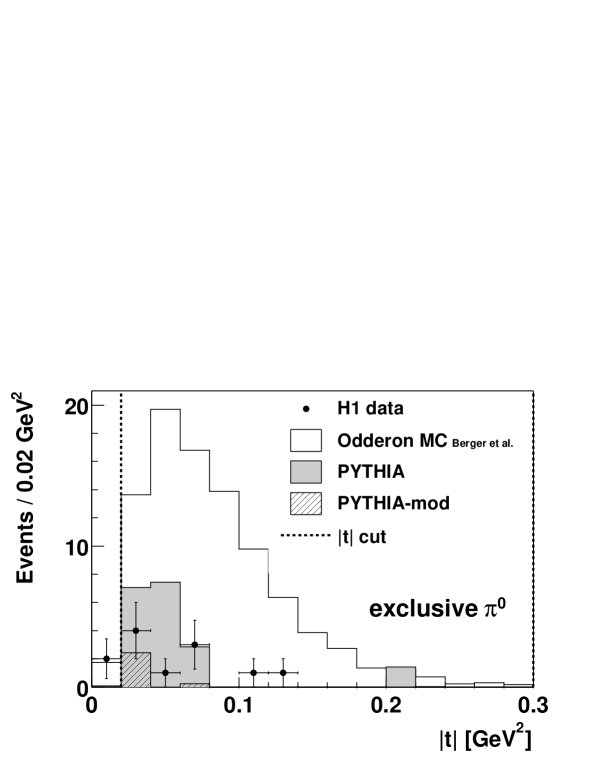
Figure 28: Measured $t$-distribution for Odderon candidate events with $M_{\gamma\gamma}<335\,\mbox{MeV}$; figure from [7]

The data are clearly in agreement with background expectations, and there is no sign of an Odderon induced production of pions. Preliminary data are also available for the production of $a_{2}$ and $f_{2}$ tensor mesons [285, 286]. Also here no signal has been observed, and the upper bounds for the cross sections are

$$\sigma(\gamma p\to a_{2}N^{*}) = 96\,\mbox{nb}$$ (4.54)

$$\sigma(\gamma p\to f_{2}N^{*}) = 16\,\mbox{nb}\,.$$ (4.55)

These bounds are again below the expectations (4.51) and (4.52), but not as significantly as in the case of $\pi^{0}$ mesons. In all three cases the reason for the failure of the prediction made in the framework of the stochastic vacuum model is unclear. In principle, there are uncertainties related to the couplings of the Odderon and to its energy dependence. It was pointed out in [7] that the experimental bounds would be reconciled with the theoretical expectations if the latter are scaled down using an energy dependence of the Odderon given by an intercept of $\alpha_{\mbox{\scriptsize{\rm\kern 1.68004pt\vrule width=0.14003pt,height=4.37012pt,depth=-0.1507pt\kern-1.81996ptO}}}(0)=0.7$. As we have discussed in section 3.4 such an intercept is certainly possible for the soft Odderon. It would clearly seem premature to draw any firm conclusions concerning the existence of the Odderon from these experimental findings. One should keep in mind that the diffractive photoproduction of pions is a very soft process, and probably the most difficult Odderon mediated process to describe in QCD. It will be very interesting to see whether the experimental bounds can be improved in the case of the tensor mesons, where they are still in the range of the theoretical expectations.

In view of the large uncertainties in the predictions for the photoproduction of light mesons it is natural to consider also cases which can be treated perturbatively. One possibility is the electroproduction of mesons of large or intermediate mass at sufficiently large photon virtuality. The other possibility is to concentrate on the diffractive production of heavy mesons like the $\eta_{c}$. In the latter case the meson mass provides a hard scale that makes a perturbative calculation possible even in the photoproduction limit.

Such calculations have been performed for the photo- or electroproduction of $\eta_{c}$ mesons [115], [287]–[289], or the leptoproduction of $f_{2}(1270)$ or $\eta(548)$ mesons [290]. Here we will discuss as an example the case of $\eta_{c}$ mesons. Again we consider the exclusive diffractive production of these mesons with the constraint that the proton stays intact. The perturbative calculation involves as a new element the $\gamma\eta_{c}{\rm\kern 2.40005pt\vrule width=0.20004pt,height=6.24301pt,depth=-0.21529pt\kern-2.59995ptO}$ impact factor. It was calculated for the first time in [288]. It carries a vector index $\mu$ due to the photon entering it. It turns out that only its transverse components $\mu=i$ ($i=1,2$) are different from zero. One of the diagrams contributing to the impact factor is shown in figure 29.

Figure 29: One of the diagrams contributing to the $\gamma^{(*)}\eta_{c}{\rm\kern 2.40005pt\vrule width=0.20004pt,height=6.24301pt,depth=-0.21529pt\kern-2.59995ptO}$ impact factor

Again, the gluons have to be attached to the quark lines in all possible ways in order to ensure gauge invariance. Using again ${\bf q}={\bf k}_{1}+{\bf k}_{2}+{\bf k}_{3}$ the impact factor becomes

$$\phi_{\gamma}^{i}=b\,\epsilon_{ij}\frac{q_{j}}{{\bf q}^{2}}\left(\frac{{\bf q}^{2}}{{\bf q}^{2}+Q^{2}+4m_{c}^{2}}+\sum_{k=1}^{3}\frac{(2{\bf k}_{k}-{\bf q})\cdot{\bf q}}{(2{\bf k}_{k}-{\bf q})^{2}+Q^{2}+4m_{c}^{2}}\right)\,,$$ (4.56)

where

$$b=\frac{16}{\pi}e_{c}g_{s}^{3}\,\frac{1}{2}\,m_{\eta_{c}}b_{0}\,,$$ (4.57)

with $m_{\eta_{c}}=2.98\,\mbox{GeV}$, $m_{c}=1.4\,\mbox{GeV}$, and $b_{0}$ is related to the radiative width $\Gamma_{\eta_{c}\to\gamma\gamma}=7\,\mbox{keV}$ of the $\eta_{c}$ meson,

$$b_{0}=\frac{16\pi^{3}}{3e_{c}^{2}}\sqrt{\frac{\pi\Gamma_{\eta_{c}\to\gamma\gamma}}{m_{\eta_{c}}}}\,.$$ (4.58)

With this impact factor at hand one can use the usual perturbative framework as described in section 4.2. In [288, 289] the Odderon is described by the perturbative exchange of three non–interacting gluons. The ${\rm\kern 2.40005pt\vrule width=0.20004pt,height=6.24301pt,depth=-0.21529pt\kern-2.59995ptO}p$ coupling is described by the Fukugita–Kwieciński form factor (4.33) with the choice $\alpha_{s}=1$ for the strong coupling constant. The two papers use slightly different choices for $\alpha_{s}$ in the $\gamma\eta_{c}{\rm\kern 2.40005pt\vrule width=0.20004pt,height=6.24301pt,depth=-0.21529pt\kern-2.59995ptO}$ impact factor. The calculations give total cross sections of around $11\,\mbox{pb}$ for photoproduction and only $0.1\,\mbox{pb}$ at a photon virtuality of $Q^{2}=25\,\mbox{GeV}^{2}$. These cross sections are energy independent due to the simple model of three non–interacting gluons for the Odderon.

In [115] the same process was calculated using a solution of the BKP equation for the Odderon. This was the first phenomenological application of a resummed Odderon solution. The authors first noticed that one cannot use the Janik–Wosiek solution in this process because its coupling to the $\gamma\eta_{c}{\rm\kern 2.40005pt\vrule width=0.20004pt,height=6.24301pt,depth=-0.21529pt\kern-2.59995ptO}$ impact factor (4.56) vanishes. This is due to the special dependence of the impact factor on the transverse momenta of the gluons. One can easily see that in each term of the impact factor two gluon momenta enter only as a sum. The Fourier transformation of such a term to impact parameter space yields a delta function of the difference of the two corresponding gluon coordinates. But this delta function immediately implies that any Odderon solution of the form (3.76) vanishes when convoluted with this impact factor, and this applies in particular to the Janik–Wosiek solution. We should add here that this decoupling of the JW solution from the $\gamma\eta_{c}{\rm\kern 2.40005pt\vrule width=0.20004pt,height=6.24301pt,depth=-0.21529pt\kern-2.59995ptO}$ impact factor according to the argument just given holds only in leading order, i. e. in the approximation that the impact factor is represented by a quark loop diagram, see figure 29. In higher order diagrams there will be gluon corrections to the loop diagram, and these can give a nonvanishing contribution to the $\gamma\eta_{c}{\rm\kern 2.40005pt\vrule width=0.20004pt,height=6.24301pt,depth=-0.21529pt\kern-2.59995ptO}$ impact factor. The situation turns out to be different for the Bartels–Lipatov–Vacca solution of the BKP equation. This solution does couple to the $\gamma\eta_{c}{\rm\kern 2.40005pt\vrule width=0.20004pt,height=6.24301pt,depth=-0.21529pt\kern-2.59995ptO}$ impact factor (4.56) already in leading order. However, it has an intercept of exactly one and one would hence expect only a small effect in comparison to the exchange of three non–interacting gluons. Surprisingly though, it was found that using exactly the same parameters as in [288] the cross section for diffractive $\eta_{c}$ production is enhanced by about an order of magnitude due to the use of the resummed Odderon solution. The total cross section now becomes $\sim 50\,\mbox{pb}$ for photoproduction, and $1.3\,\mbox{pb}$ at a photon virtuality of $Q^{2}=25\,\mbox{GeV}$. The corresponding differential cross section is shown in figure 30.

Figure 30: The differential cross sections for exclusive diffractive $\eta_{c}$ production according to [115]. The upper curve refers to $Q^{2}=0$, the lower curve to $Q^{2}=25\,\mbox{GeV}^{2}$.

The dip in the differential cross section occurs only when the BLV solution for the Odderon is used, but is absent in the calculations [288, 289] where the Odderon is modeled by three non-interacting gluons. In all three calculations the differential cross section vanishes in the exact forward direction $t=0$, but starts to decrease only at very small $|t|$ such that this property is not visible in figure 30. Due to that fact the cross section is at small $|t|$ dominated by photon exchange. The very forward direction is hence not well suited for finding the Odderon in this process.

It should be pointed out that all three perturbative calculations of this process have been performed assuming a coupling constant $\alpha_{s}=1$ in the ${\rm\kern 2.40005pt\vrule width=0.20004pt,height=6.24301pt,depth=-0.21529pt\kern-2.59995ptO}p$ impact factor. According to the findings of [213] this is a very optimistic choice. Calculating the differential cross section for elastic $pp$ scattering in the dip region, which corresponds to an at least similar kinematical situation, one finds that this value if far too large, and $\alpha_{s}\simeq 0.3$ would be more appropriate, see figure 15 and the corresponding discussion in section 4.3.2. We recall here that the difference between these two values for $\alpha_{s}$ causes a large difference for the cross section since the squared Odderon–proton impact factor entering it is proportional to $\alpha_{s}^{3}$, and the more realistic choice of $\alpha_{s}\simeq 0.3$ would reduce the cross section by a factor of about $30$. With this more realistic estimate the perturbatively calculated cross sections are in a range similar to the estimate obtained using the framework of Regge theory in [281], see above.

In an alternative approach one can make use of the large mass of the charm quark to describe the diffractive production of $\eta_{c}$ mesons using techniques typical for treating heavy quarks. This approach has been pursued in [291] where the photoproduction region of this process was considered. The $\eta_{c}$ meson is treated in the framework of nonrelativistic QCD, and heavy quark effective theory is used to describe the exchange of soft gluons. Then a systematic expansion in inverse powers of the charm mass $m_{c}$ can be applied. The cross section can be expressed in terms of four functions parametrizing the matrix element of a twist-3 gluon operator taken between the ingoing and outgoing proton states. These four functions are of nonperturbative origin and are presently not known numerically. A rough estimate of the diffractive $\eta_{c}$ photoproduction cross section is possible though when the process is compared to the diffractive photoproduction of $J/\psi$ mesons, which has been studied in the same framework in [291]. Such a rough estimate gives a differential cross section of $2\,\mbox{nb}/\mbox{GeV}^{2}$ in the forward direction $t=0$ at HERA. This is at least an order of magnitude larger than the values obtained in the perturbative approach [288, 289, 115], and may be even larger when a smaller coupling in the Odderon–proton impact factor is chosen in those calculations. Interestingly, it is found in the approach of [291] that in contrast to the perturbative results the cross section for this process due to Odderon exchange does not vanish in the limit $t=0$.

Even with an optimistic choice of $\alpha_{s}$ the cross section for diffractive $\eta_{c}$ production is unfortunately too small to be observed at HERA. Nevertheless, the investigation of this process is very instructive for the following reasons. It has been found here that the $\gamma{\rm\kern 2.40005pt\vrule width=0.20004pt,height=6.24301pt,depth=-0.21529pt\kern-2.59995ptO}\eta_{c}$ impact factor has a very special dependence on the three gluon momenta. As a consequence, it does not couple to the Janik–Wosiek solution of the BKP equation for the Odderon. But it does couple to the Bartels–Lipatov–Vacca solution. This observation is quite relevant for the interpretation of different types of solutions of the BKP equation, and in fact it probably implies that the Hilbert space for admissible solutions of the BKP equations has to be extended as compared to previous assumptions, see also section 3.2.6. In addition, it is a very interesting result that the inclusion of the resummed Odderon solution increases the cross section as compared to the exchange of three non–interacting gluons. This is very unexpected since the BLV solution used here has an intercept exactly equal to one, i. e. has the same intercept as the exchange of three non–interacting gluons. It is conceivable that the use of resummed Odderon solutions might in general lead to higher cross sections also in other processes. It would be very important to study this question in more detail.

So far we have considered the diffractive production of pseudoscalar and tensor mesons under the assumption that the proton stays intact or is excited into a small–mass state. A very interesting possibility is the other extreme, namely the case in which the proton breaks up into a large–mass system $X$. The breakup of the proton into a large–mass system certainly reduces the probability of having a rapidity gap, but there should still be a considerable fraction of events left which have a rapidity gap in the final state between the meson and the large–mass proton remnant, ensuring that the reaction is mediated by Odderon exchange. The corresponding amplitude is shown on the left hand side of figure 31.

Figure 31: The Pomeron–Odderon–Odderon vertex in diffractive production of pseudoscalar mesons with a breakup of the proton into a large–mass system

The large–mass system is generated mainly by gluon emissions. If one now squares this amplitude to obtain the cross section for this process (right hand side in figure 31) one finds that the cross section involves the Pomeron–Odderon–Odderon (${\rm I\kern-2.5ptP}{\rm\kern 2.40005pt\vrule width=0.20004pt,height=6.24301pt,depth=-0.21529pt\kern-2.59995ptO}{\rm\kern 2.40005pt\vrule width=0.20004pt,height=6.24301pt,depth=-0.21529pt\kern-2.59995ptO}$) vertex. The possibility of observing the ${\rm I\kern-2.5ptP}{\rm\kern 2.40005pt\vrule width=0.20004pt,height=6.24301pt,depth=-0.21529pt\kern-2.59995ptO}{\rm\kern 2.40005pt\vrule width=0.20004pt,height=6.24301pt,depth=-0.21529pt\kern-2.59995ptO}$ vertex in this process has first been mentioned in [280]. An advantage of this process is that it does not involve the poorly known coupling of the Odderon to the proton. Instead it involves the coupling of the two Odderons to the Pomeron and the comparatively well–known coupling of the Pomeron to the proton. If the diffractively produced meson is heavy, one can use perturbation theory to calculate the cross section. In particular, one can use the perturbative ${\rm I\kern-2.5ptP}{\rm\kern 2.40005pt\vrule width=0.20004pt,height=6.24301pt,depth=-0.21529pt\kern-2.59995ptO}{\rm\kern 2.40005pt\vrule width=0.20004pt,height=6.24301pt,depth=-0.21529pt\kern-2.59995ptO}$ vertex [133], see section 3.3.3. Note also that the cross section is in this case expected to be enhanced at large energies due to the occurrence of a hard Pomeron. The case of inclusive diffractive $\eta_{c}$ production, $\gamma^{(*)}+p\to\eta_{c}+X$, has been studied in [136]. Here the BLV solution for the perturbative Odderon has been used, and the perturbative ${\rm I\kern-2.5ptP}{\rm\kern 2.40005pt\vrule width=0.20004pt,height=6.24301pt,depth=-0.21529pt\kern-2.59995ptO}{\rm\kern 2.40005pt\vrule width=0.20004pt,height=6.24301pt,depth=-0.21529pt\kern-2.59995ptO}$ vertex for this solution is calculated in the large-$N_{c}$ limit. The coupling of the Pomeron to the proton can be determined using a Pomeron–based fit of the gluon density of the proton at small $x$. A suitable scale for the strong coupling in the ${\rm I\kern-2.5ptP}{\rm\kern 2.40005pt\vrule width=0.20004pt,height=6.24301pt,depth=-0.21529pt\kern-2.59995ptO}{\rm\kern 2.40005pt\vrule width=0.20004pt,height=6.24301pt,depth=-0.21529pt\kern-2.59995ptO}$ vertex is estimated based on the diffusion mechanism of the momenta in the perturbative Pomeron, see section 3.1.5. In addition to the diagram in figure 31 (representing the triple-Regge contribution) there is another contribution to this process in which the three–gluon states from the $\gamma{\rm\kern 2.40005pt\vrule width=0.20004pt,height=6.24301pt,depth=-0.21529pt\kern-2.59995ptO}\eta_{c}$ impact factors are coupled directly to the Pomeron. This second contribution comes from the part of the six–gluon amplitude $D_{6}$ which reggeizes, see section 3.3.2. Also this contribution is computed in the large-$N_{c}$ limit based on the results of [133]. Both contributions are of the same order of magnitude but behave differently with the transferred momentum. It should be pointed out that the cross section is large in the region of phase space in which the Pomeron fills the whole rapidity range between the proton and the $\eta_{c}$ meson. Therefore it would be necessary to apply suitable cuts on the rapidity in order to focus only on processes where there is an Odderon, i. e. a gap between the $\eta_{c}$ meson and the proton remnant $X$. In [136] the total cross section integrated over the mass of the system $X$ is calculated for the kinematics of HERA ($\sqrt{s}=300\,\mbox{GeV}$). In the case of photoproduction the total cross section is found to be $65\,\mbox{pb}$, whereas at $Q^{2}=25\,\mbox{GeV}^{2}$ it is only $1.5\,\mbox{pb}$. This however includes contributions with only a small or no gap between the $\eta_{c}$ and the system $X$, and it should hence only be interpreted as an estimate of the order of magnitude. As expected these cross sections are larger than those for the quasi–elastic process $\gamma^{(*)}+p\to\eta_{c}+p$ in which the proton stays intact. The difference is even more pronounced when a realistic value for $\alpha_{s}$ is chosen in that process, as has been discussed above.

4.4.2 Asymmetries

The processes discussed in the preceding section typically involve the exchange of an Odderon on the amplitude level. The corresponding cross sections are thus quadratic in the factor describing the Odderon exchange and in the couplings of the Odderon to the external particles. Both of these dependencies imply some uncertainties, in particular when we are dealing with soft processes. There might be unexpected effects hidden in the Odderon couplings as well as in the Odderon propagation, as we have seen in the case of diffractive photoproduction of $\pi^{0}$ mesons where the theoretical estimates turned out to be rather poor. It is therefore desirable to consider also observables in which these uncertainties are reduced. A class of such observables has been proposed recently. These observables make use of the fact that the Odderon can interfere with the Pomeron in suitably defined asymmetries of final state particles if the final state does not have a well–defined charge parity, for example if the final state consists of a pair of charged pions which can be in a $C=+1$ state as well as in a $C=-1$ state. The asymmetry is then proportional to the product of the amplitudes for Pomeron and for Odderon exchange, and thus linear in the Odderon amplitude. Since the Pomeron is a comparatively well–understood object such asymmetries are expected to have a much smaller uncertainty caused by the unknowns of the Odderon. Moreover, some of the asymmetries discussed so far are estimated to be large enough to offer a substantial discovery potential for the Odderon in these observables at HERA.

The first example of such an asymmetry was proposed in [292]. We will use it to explain the basic idea behind the Pomeron–Odderon interference. Consider the diffractive production of a charm quark–antiquark pair as sketched in figure 32.

Figure 32: Mechanism for the diffractive production of a $c\bar{c}$ pair

Here the photon can be either real or virtual. To be specific we consider the case of real photons in which also the expected cross sections are larger. A $c\bar{c}$ pair as such is not necessarily an eigenstate of charge conjugation $C$. The pair can be produced in a $C=-1$ state via Pomeron exchange as well as in a $C=+1$ state via Odderon exchange. We denote the amplitudes for the two production mechanism as $A_{\mbox{\scriptsize{\rm I\kern-1.75ptP}}}$ and $A_{\mbox{\scriptsize{\rm\kern 1.68004pt\vrule width=0.14003pt,height=4.37012pt,depth=-0.1507pt\kern-1.81996ptO}}}$, respectively. In the calculation of total cross sections the two amplitudes do obviously not interfere. However, on the level of the differential cross section there is still an interference term,

$$d\sigma=|A|^{2}=|A_{\mbox{\scriptsize{\rm I\kern-1.75ptP}}}+A_{\mbox{\scriptsize{\rm\kern 1.68004pt\vrule width=0.14003pt,height=4.37012pt,depth=-0.1507pt\kern-1.81996ptO}}}|^{2}=|A_{\mbox{\scriptsize{\rm I\kern-1.75ptP}}}|^{2}+2\mbox{Re}\,(A_{\mbox{\scriptsize{\rm I\kern-1.75ptP}}}A_{\mbox{\scriptsize{\rm\kern 1.68004pt\vrule width=0.14003pt,height=4.37012pt,depth=-0.1507pt\kern-1.81996ptO}}}^{*})+|A_{\mbox{\scriptsize{\rm\kern 1.68004pt\vrule width=0.14003pt,height=4.37012pt,depth=-0.1507pt\kern-1.81996ptO}}}|^{2}\,.$$ (4.59)

The idea is to isolate this interference term in suitable asymmetries defined through differential cross sections. A first look at the interference term tells us that it is expected to be small. The reason lies in the fact that Pomeron exchange gives a predominantly imaginary contribution to the amplitude while Odderon exchange gives a predominantly real contribution. Hence the two contributions are almost orthogonal to each other and the interference term is small. As we have seen in section 2.2 this orthogonality of the two contributions is even exact in the case of two Regge poles for the Pomeron and Odderon with exactly the same intercept. We therefore expect that the asymmetries constructed from the interference term vanish in the limit $\alpha_{\mbox{\scriptsize{\rm\kern 1.68004pt\vrule width=0.14003pt,height=4.37012pt,depth=-0.1507pt\kern-1.81996ptO}}}\to\alpha_{\mbox{\scriptsize{\rm I\kern-1.75ptP}}}$. However, it turns out that this cancellation is effective only on the parton level, as was observed in [293]. If one considers asymmetries on the hadron level (see the example of di–pion production below) there are additional Breit–Wigner phases associated with the formation of the hadrons which can eliminate the cancellation. This should be especially important for light hadrons, and probably would have little effect in charm production. In addition, we do not expect the Pomeron and Odderon intercepts to be equal and hence one can hope to see an effect also in the process of diffractive open charm production, to which we now return.

In [292] it was shown that the charge asymmetry

$${\cal A}(t,M_{x}^{2},z_{c})=\frac{{\displaystyle\frac{d\sigma}{dt\,dM_{X}^{2}\,dz_{c}}-\frac{d\sigma}{dt\,dM_{X}^{2}\,dz_{\bar{c}}}}}{{\displaystyle\frac{d\sigma}{dt\,dM_{X}^{2}\,dz_{c}}+\frac{d\sigma}{dt\,dM_{X}^{2}\,dz_{\bar{c}}}}}$$ (4.60)

is in fact proportional to the interference term of the Pomeron and Odderon amplitudes. Here $M_{X}$ is the invariant mass of the charm quark–antiquark pair, and $z_{c}$ ($z_{\bar{c}}$) denotes the momentum sharing of the $c\bar{c}$ pair. Denoting the photon momentum by $q$ and the proton momentum by $p$, and the charm quark (antiquark) momentum by $p_{c}$ ($p_{\bar{c}}$) we have

$$z_{c}=\frac{p_{c}\cdot p}{q\cdot p}\,,$$ (4.61)

and an analogous relation for the antiquark. $z_{c}+z_{\bar{c}}=1$ holds in Born approximation on the parton level. We are interested in the kinematic region of a large energy of the $\gamma p$ system, $s_{\gamma p}\gg M_{X}^{2}$. The authors of [292] use a Regge picture of the Pomeron and Odderon to estimate the asymmetry (4.60) which can then be expressed as

$${\cal A}(t,M_{x}^{2},z_{c})=\frac{{\displaystyle g^{\mbox{\scriptsize{\rm I\kern-1.75ptP}}}_{pp^{\prime}}g^{\mbox{\scriptsize{\rm\kern 1.68004pt\vrule width=0.14003pt,height=4.37012pt,depth=-0.1507pt\kern-1.81996ptO}}}_{pp^{\prime}}\left(\frac{s_{\gamma p}}{M_{X}^{2}}\right)^{\alpha_{\mbox{\tiny{\rm I\kern-1.25ptP}}}+\alpha_{\mbox{\tiny{\rm\kern 1.20003pt\vrule width=0.10002pt,height=3.1215pt,depth=-0.10764pt\kern-1.29997ptO}}}}\frac{2\sin\left[\frac{\pi}{2}(\alpha_{\mbox{\tiny{\rm\kern 1.20003pt\vrule width=0.10002pt,height=3.1215pt,depth=-0.10764pt\kern-1.29997ptO}}}-\alpha_{\mbox{\tiny{\rm I\kern-1.25ptP}}})\right]}{\sin\frac{\pi\alpha_{\mbox{\tiny{\rm I\kern-1.25ptP}}}}{2}\cos\frac{\pi\alpha_{\mbox{\tiny{\rm\kern 1.20003pt\vrule width=0.10002pt,height=3.1215pt,depth=-0.10764pt\kern-1.29997ptO}}}}{2}}\,\,g_{\mbox{\scriptsize{\rm I\kern-1.75ptP}}}^{\gamma c\bar{c}}g_{\mbox{\scriptsize{\rm\kern 1.68004pt\vrule width=0.14003pt,height=4.37012pt,depth=-0.1507pt\kern-1.81996ptO}}}^{\gamma c\bar{c}}}}{{\displaystyle\left[g^{\mbox{\scriptsize{\rm I\kern-1.75ptP}}}_{pp^{\prime}}\left(\frac{s_{\gamma p}}{M_{X}^{2}}\right)^{\alpha_{\mbox{\tiny{\rm I\kern-1.25ptP}}}}g_{\mbox{\scriptsize{\rm I\kern-1.75ptP}}}^{\gamma c\bar{c}}/\sin\frac{\pi\alpha_{\mbox{\tiny{\rm I\kern-1.25ptP}}}}{2}\right]^{2}+\left[g^{\mbox{\scriptsize{\rm\kern 1.68004pt\vrule width=0.14003pt,height=4.37012pt,depth=-0.1507pt\kern-1.81996ptO}}}_{pp^{\prime}}\left(\frac{s_{\gamma p}}{M_{X}^{2}}\right)^{\alpha_{\mbox{\tiny{\rm\kern 1.20003pt\vrule width=0.10002pt,height=3.1215pt,depth=-0.10764pt\kern-1.29997ptO}}}}g_{\mbox{\scriptsize{\rm\kern 1.68004pt\vrule width=0.14003pt,height=4.37012pt,depth=-0.1507pt\kern-1.81996ptO}}}^{\gamma c\bar{c}}/\cos\frac{\pi\alpha_{\mbox{\tiny{\rm\kern 1.20003pt\vrule width=0.10002pt,height=3.1215pt,depth=-0.10764pt\kern-1.29997ptO}}}}{2}\right]^{2}}}\,,$$ (4.62)

where the meaning of the different couplings $g_{{\mbox{\scriptsize{\rm I\kern-1.75ptP}}}/{\mbox{\scriptsize{\rm\kern 1.68004pt\vrule width=0.14003pt,height=4.37012pt,depth=-0.1507pt\kern-1.81996ptO}}}}$ should be evident. We see that as expected the asymmetry is proportional to $\sin[(\alpha_{\mbox{\scriptsize{\rm\kern 1.68004pt\vrule width=0.14003pt,height=4.37012pt,depth=-0.1507pt\kern-1.81996ptO}}}-\alpha_{\mbox{\scriptsize{\rm I\kern-1.75ptP}}})\pi/2]$ and thus vanishes if the two intercepts are equal. One now assumes that the Pomeron and the Odderon are coupled to the charm quark and antiquark individually and to the single quarks in the proton according to (4.29) and (4.30), respectively. The dependence of the asymmetry on $z_{c}$ and $z_{\bar{c}}$ enters while coupling the Pomeron and Odderon separately to the charm quark and antiquark. The authors then further consider $t\simeq 0$ and use for the (hard) Pomeron and Odderon intercepts the values $\alpha_{\mbox{\scriptsize{\rm I\kern-1.75ptP}}}=1.2$ and $\alpha_{\mbox{\scriptsize{\rm\kern 1.68004pt\vrule width=0.14003pt,height=4.37012pt,depth=-0.1507pt\kern-1.81996ptO}}}=0.95$, respectively. . They estimate the relative couplings of the Pomeron and Odderon to the proton as $g^{\mbox{\scriptsize{\rm\kern 1.68004pt\vrule width=0.14003pt,height=4.37012pt,depth=-0.1507pt\kern-1.81996ptO}}}_{pp^{\prime}}/g^{\mbox{\scriptsize{\rm I\kern-1.75ptP}}}_{pp^{\prime}}=0.1$, and assume for their relative coupling to the charm quark $\kappa_{\mbox{\scriptsize{\rm\kern 1.68004pt\vrule width=0.14003pt,height=4.37012pt,depth=-0.1507pt\kern-1.81996ptO}}}^{\gamma c\bar{c}}/\kappa_{\mbox{\scriptsize{\rm I\kern-1.75ptP}}}^{\gamma c\bar{c}}=0.6$. Then the asymmetry becomes

$${\cal A}(t\simeq 0,M_{x}^{2},z_{c})\simeq 0.45\,\left(\frac{s_{\gamma p}}{M_{X}^{2}}\right)^{-0.25}\frac{2z_{c}-1}{z_{c}^{2}+(1-z_{c})^{2}}\,.$$ (4.63)

For a typical value of $s_{\gamma p}/M_{X}^{2}=100$ this results in a $\sim 15\%$ asymmetry for large $z_{c}$ as illustrated in figure 33.

Figure 33: The asymmetry in fractional energy $z_{c}$ of the charm versus the anticharm jets for $s_{\gamma p}/M_{X}^{2}=100$; figure from [292]

It should be emphasized that the estimates for the different couplings made here are quite uncertain. Experimentally, the identification of charm quarks is nontrivial, and the measurement of the fractional energy of charm jets in diffraction is very challenging. Therefore the charge asymmetry for diffractive open charm production is probably not the best possible asymmetry for actually finding an Odderon effect. But it is conceptually the simplest, and therefore we have chosen to present it in some detail here.

Better prospects for an actual discovery of an Odderon–Pomeron interference effect at HERA can be expected from the exclusive diffractive production of charged pion pairs. The process is in principle similar to the production of open charm in figure 32, but now one considers the production of a $\pi^{+}\pi^{-}$ pair instead of a $c\bar{c}$ pair. Again, the pion pair can be produced in a $C=+1$ state via Odderon exchange as well as in a $C=-1$ state via Pomeron exchange. One can construct different asymmetries involving the interference term of the two corresponding amplitudes. Asymmetries in this process have been studied both in electroproduction [294, 295] and in photoproduction [293, 296]. The advantage of photoproduction is clearly the much larger cross section for this process. In electroproduction, on the other hand, the large photon virtuality allows one to calculate the process in a perturbative approach which is under better theoretical control.

Let us first consider the case of electroproduction. In [294] only the contribution of longitudinally polarized photons was considered which dominate at very large photon virtualities $Q^{2}$. In this approximation the charge asymmetry of the pion pair was calculated. In [295] this calculation was improved by also taking into account the contribution of transversely polarized photons. With the latter contribution it was also possible to calculate a spin asymmetry which only occurs as an interference effect between longitudinally and transversely polarized photons. The calculation of the Pomeron and Odderon amplitudes is done using the perturbative exchange of two or three non–interacting gluons, respectively. The coupling of the Odderon to the proton is modeled using the Fukugita–Kwieciński form factor (4.33), and a similar model is used for the Pomeron–proton impact factor. The $\gamma^{*}{\rm\kern 2.40005pt\vrule width=0.20004pt,height=6.24301pt,depth=-0.21529pt\kern-2.59995ptO}\pi^{+}\pi^{-}$ and $\gamma^{*}{\rm I\kern-2.5ptP}\pi^{+}\pi^{-}$ impact factors are calculated by coupling the three or two perturbative gluons to a quark–antiquark pair in all possible ways, and the resulting expression is then convoluted with appropriate generalized two pion distribution amplitudes (GDAs) [297]–[300]. They describe the transition of the $q\bar{q}$ pair into the $\pi^{+}\pi^{-}$ final state. The one used in the Odderon amplitude involves the $s$ and $d$ wave contributions corresponding to $f_{0}$ and $f_{2}$ meson poles in the $\pi\pi$ elastic amplitude. The GDA for the Pomeron amplitude involves the $p$ wave described by the phase shift and Breit–Wigner distribution for the $\rho$ meson. The GDAs are nonperturbative objects which contain the full information about the production of the pion pair in the final state. Accordingly, there is a large theoretical uncertainty related to these amplitudes which is rather difficult to estimate. The charge asymmetry is defined as

$${\cal A_{C}}(Q^{2},t,m_{\pi^{+}\pi^{-}}^{2},y,\alpha)=\frac{{\displaystyle\sum_{\lambda=\pm}\int\cos\theta\,d\sigma(s,Q^{2},t,m_{\pi^{+}\pi^{-}}^{2},y,\alpha,\theta,\lambda)}}{{\displaystyle\sum_{\lambda=\pm}\int d\sigma(s,Q^{2},t,m_{\pi^{+}\pi^{-}}^{2},y,\alpha,\theta,\lambda)}}\,,$$ (4.64)

where $s$ is the squared energy of the photon–proton system, $y$ is the fractional energy loss of the electron, $\alpha$ is the angle between the electron scattering plane and the hadronic scattering plane, $\theta$ is the polar angle of the $\pi^{+}$ in the dipion rest frame, and $\lambda$ is the initial electron helicity. Note that in the approximation used in [294, 295] the charge asymmetry ${\cal A_{C}}$ is independent of $\sqrt{s}$ at sufficiently large energies. In figure 34 we show the numerical results [295] for the charge asymmetry as a function of the two–pion invariant mass and for values for the other parameters which are typical for the HERA kinematic region.

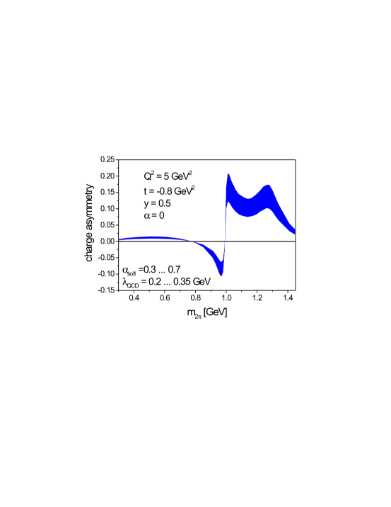
Figure 34: Charge asymmetry in the diffractive electroproduction of charged pion pairs at $Q^{2}=5\,\mbox{GeV}^{2}$ as a function of the dipion mass $m_{2\pi}$; figure from [295]

The error band corresponds to a variation of $\Lambda_{\mbox{\scriptsize QCD}}$ and of the strong coupling constant in the ${\rm\kern 2.40005pt\vrule width=0.20004pt,height=6.24301pt,depth=-0.21529pt\kern-2.59995ptO}p$ impact factor. Here the values of the strong coupling were chosen in a range compatible with the results obtained for the Odderon–proton coupling obtained in the description of $pp$ elastic scattering in [213], see section 4.3.2. It was found that the size of the charge asymmetry decreases with increasing photon virtuality $Q^{2}$. When going from $Q^{2}=3\,\mbox{GeV}^{2}$ to $Q^{2}=10\,\mbox{GeV}^{2}$, for example, the charge asymmetry varies roughly in the range of the band in figure 34. The shape of the asymmetry as a function of the dipion mass, however, is almost invariant under changes in $Q^{2}$. Depending on the dipion mass the charge asymmetry is sizable and in a range that could well be accessible experimentally. The shape of the charge distribution can largely be understood in terms of the $\pi\pi$ phase shifts. It is largest around the $f_{0}$ and $f_{2}$ masses. Especially the zeros of the charge asymmetry should be robust against changes in most of the parameters.

The single spin asymmetry

$${\cal A_{S}}(Q^{2},t,m_{\pi^{+}\pi^{-}}^{2},y,\alpha)=\frac{{\displaystyle\sum_{\lambda=\pm}\lambda\int\cos\theta\,d\sigma(s,Q^{2},t,m_{\pi^{+}\pi^{-}}^{2},y,\alpha,\theta,\lambda)}}{{\displaystyle\sum_{\lambda=\pm}\int d\sigma(s,Q^{2},t,m_{\pi^{+}\pi^{-}}^{2},y,\alpha,\theta,\lambda)}}\,.$$ (4.65)

has been calculated in the same way, and its dependence on the dipion mass is shown in figure 35.

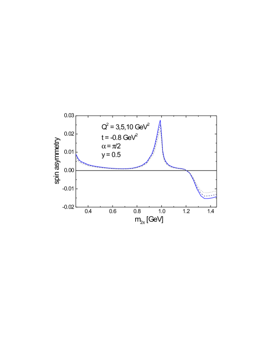
Figure 35: Single spin asymmetry in the diffractive electroproduction of charged pion pairs as a function of the dipion mass for different photon virtualities $Q^{2}$; figure from [295]

The figure clearly shows that the spin asymmetry depends only very weakly on the photon virtuality. The spin asymmetry is considerably smaller than the charge asymmetry. An experimental verification of the Odderon in the spin asymmetry will hence be rather difficult.

A similar analysis for the diffractive photoproduction of a charged pion pair was performed in [293, 296] in the framework of Regge theory. Again it is crucial to observe that the Pomeron amplitude for the production of a pion pair is dominated by the intermediate formation of a $\rho$ meson, whereas the Odderon amplitude is dominated by the $f_{2}(1270)$ resonance in the region above $\sim 1\,\mbox{GeV}$. Accordingly, the result can be expressed in terms of an overlap function involving the Breit–Wigner distributions of the respective resonances. An important ingredient is the production cross section for $f_{2}$ mesons, $\sigma(\gamma p\to f_{2}p)$, which is assumed to be larger than $1\,\mbox{nb}$. In addition to the charge asymmetry the authors of [296] study also the transverse asymmetry and a forward–backward asymmetry. They conclude that especially the charge asymmetry should lead to a very significant effect in the dipion mass region of $1.1\!-\!1.5\,\mbox{GeV}$. It should again be emphasized that in the case of diffractive dipion production the orthogonality of the Odderon and Pomeron contributions at the parton level is lifted when going to the hadron level due to the additional Breit–Wigner phases occurring in the hadronization. In a sense the large expected effects in the charge asymmetry can thus be viewed as a maximal violation of parton–hadron duality. One should here be able to observe an effect on the hadron level which is almost absent on the parton level.

4.5 Photon-Photon Processes

In all processes that we have considered so far one of the largest uncertainties comes from the coupling of the Odderon to the proton which is of nonperturbative nature and cannot be calculated from first principles. Moreover, it is well possible that this coupling is very small, and different possible mechanism for this have been discussed in section 4.3.1. The processes which we want to discuss now are not affected by this problem. Moreover, they can in many cases be calculated perturbatively. Therefore photon–photon processes can be considered the cleanest possible test of the Odderon, at least from a theoretical perspective.

Photon–photon scattering occurs as a subprocess in electron–positron collisions when both the electron and the positron radiate a photon,

$$e^{+}e^{-}\longrightarrow e^{+}e^{-}\gamma^{(*)}\gamma^{(*)}\,,$$ (4.66)

with the subsequent reaction of the two photons. Here the photons can be both real or virtual, or one can be real and the other one can be virtual. In the following we will only consider the subsequent scattering of the two photons. If the electron or positron are tagged in the detector one is in a position to reconstruct the four–momenta of the photons and their virtuality. By implementing suitable cuts on the photon virtualities in tagged events one can select only events in which both photons are virtual.

The process of interest for the Odderon is the quasi–diffractive production of pseudoscalar or tensor mesons. Here it is possible that two pseudoscalar or tensor mesons are produced,

$$\gamma^{(*)}\gamma^{(*)} \longrightarrow M_{\mbox{\scriptsize PS }}+M_{\mbox{\scriptsize PS }}$$ (4.67)

$$\gamma^{(*)}\gamma^{(*)} \longrightarrow M_{\mbox{\scriptsize T}}+M_{\mbox{\scriptsize T }}\,,$$ (4.68)

where for the pseudoscalar mesons we can have for example $M_{\mbox{\scriptsize PS }}=\pi$, $\eta$, $\eta^{\prime}$, or $\eta_{c}$. For the tensor mesons one can consider for instance $M_{\mbox{\scriptsize T}}=a_{2}$ or $f_{2}$. It is also possible that only one pseudoscalar or tensor meson is produced quasidiffractively while the other photon dissociates into a hadronic system $X$ of small mass,

$$\gamma^{(*)}\gamma^{(*)}\longrightarrow M_{\mbox{\scriptsize PS/T}}+X\,.$$ (4.69)

In all of these processes the momentum transfer should be small compared to the energy of the two–photon system. In this case all of the above processes can only be caused by Odderon or photon exchange, and the exchange of photons is theoretically well–understood. Due to the quantum numbers of the produced mesons Pomeron exchange is excluded.

In the case of heavy meson production, like for example for $\eta_{c}$ mesons, the meson mass provides a hard scale in the process and one can apply perturbation theory even in the case of real photons. For the production of light mesons one can in double–tagged events choose to consider only the scattering of two highly virtual photons such that again perturbation theory can be applied. In theses cases the Odderon can safely be modeled by the exchange of three gluons. So far this has been done only using three non–interacting gluons, but in an improved calculation one could also make use of the known solutions of the BKP equation.

Early studies of the above processes have been performed in [280, 301, 302]. The processes of interest have a rather small cross section in particular in situations where we can apply perturbation theory. This is either due to the restricted phase space for the production of heavy mesons, or due to the strong suppression of photon fluxes when one goes from real to virtual photons. Unfortunately, the energy of the LEP collider was not sufficient to study the Odderon in photon–photon interactions there. Accordingly, the interest in these processes was low for quite some time. Renewed interest was raised in the light of plans for a future linear $e^{+}e^{-}$-collider with a center–of-mass energy of $\sqrt{s}=500\,\mbox{GeV}$ with a very high luminosity. Such a machine would in fact offer excellent opportunities for studying high energy QCD. Some processes of interest for Pomeron physics have already been mentioned in section 3.1.5. For the Odderon it is likely that all of the processes mentioned above can be observed at such a linear collider.

Let us consider as an example the production of $\eta_{c}$ mesons as it has been studied in [303]. The amplitude for $\gamma\gamma\to\eta_{c}\eta_{c}$ is calculated perturbatively according to (4.2) and the Odderon is modeled by the exchange of three non–interacting gluons according to (4.3). The $\gamma^{(*)}\eta_{c}{\rm\kern 2.40005pt\vrule width=0.20004pt,height=6.24301pt,depth=-0.21529pt\kern-2.59995ptO}$ impact factors are calculated as described in section 4.4.1, see figure 29. In the case of the reaction $\gamma\gamma\to\eta_{c}X$ one has to use in addition the $\gamma X{\rm\kern 2.40005pt\vrule width=0.20004pt,height=6.24301pt,depth=-0.21529pt\kern-2.59995ptO}$ impact factor which can also be computed perturbatively. One of the diagrams for this impact factor is shown in figure 36,

Figure 36: One of the diagrams contributing to the $\gamma^{(*)}X{\rm\kern 2.40005pt\vrule width=0.20004pt,height=6.24301pt,depth=-0.21529pt\kern-2.59995ptO}$ impact factor

and here again the gluons have to be attached to the quark lines in all possible ways in order to arrive at a gauge invariant expression.

In [303] the case of real photons is considered. The differential cross sections for the two processes due to Odderon exchange are shown in figure 37.

Figure 37: Differential cross section for the processes $\gamma\gamma\to\eta_{c}\eta_{c}$ (a) and $\gamma\gamma\to\eta_{c}X$ (b); figure from [303]

The total cross sections for the two processes are $\sigma_{T}^{\eta_{c}\eta_{c}}=43\,\mbox{fb}$, and $\sigma_{T}^{\eta_{c}X}(|t|>3\,\mbox{GeV}^{2})=120\,\mbox{fb}$, respectively. These values are obtained assuming $\alpha_{s}(m_{c}^{2})=0.38$, and the authors of [303] assume that the strong coupling is given by $\tilde{\alpha}_{s}=0.3$ in the $\gamma^{(*)}X{\rm\kern 2.40005pt\vrule width=0.20004pt,height=6.24301pt,depth=-0.21529pt\kern-2.59995ptO}$ impact factor. We recall that the cross sections obtained using a simple three–gluon exchange model of the Odderon do not depend on the energy. For untagged events in which the electron and positron are scattered under a very small angle $\theta<30\,\mbox{mrad}$ in the detector one finds for a $\sqrt{s}=500\,\mbox{GeV}$ Linear Collider cross sections of $\sigma(e^{+}e^{-}\to e^{+}e^{-}\eta_{c}\eta_{c})=3.5\,\mbox{fb}$, and $\sigma(e^{+}e^{-}\to e^{+}e^{-}\eta_{c}X)=10\,\mbox{fb}$.

Finally, let us point out that photon–photon processes offer also the possibility of studying the Pomeron–Odderon–Odderon vertex. This is in complete analogy to the occurrence of this vertex in the diffractive production of pseudoscalar mesons in $ep$ collisions when the proton dissociates into a large–mass system, see figure 31 and the corresponding discussion in section 4.4.1. In photon–photon collisions the analogous process is the quasidiffractive production of pseudoscalar or tensor mesons

$$\gamma^{(*)}\gamma^{(*)}\longrightarrow M_{\mbox{\scriptsize PS/T}}+X\,,$$ (4.70)

with $X$ now being a large–mass system separated from the meson by a large rapidity gap. The photons can again be either real or virtual. For the case of highly virtual photons or the production of a heavy meson one can apply perturbation theory. Hence it would be possible to measure in these processes the perturbative ${\rm I\kern-2.5ptP}{\rm\kern 2.40005pt\vrule width=0.20004pt,height=6.24301pt,depth=-0.21529pt\kern-2.59995ptO}{\rm\kern 2.40005pt\vrule width=0.20004pt,height=6.24301pt,depth=-0.21529pt\kern-2.59995ptO}$ vertex [133] (see section 3.3.3). Again it is likely that the cross section for the production of a large–mass system $X$ is enhanced as compared to a small–mass system $X$.

5 Conclusions

The Odderon is an interesting object. While initially widely regarded only as a rather theoretical possibility in the framework of Regge theory its existence is now considered almost unavoidable if our QCD–based picture of high energy scattering is correct. This dramatic change in the general opinion on the Odderon was mainly caused by the impressive progress that has been made recently in perturbative studies of the Odderon. These results clearly indicated the existence of an Odderon in high energy scattering.

The perturbative Odderon can be understood as the $t$-channel exchange of three interacting reggeized gluons. In the leading logarithmic approximation it is described by the BKP equation which is the analogue of the BFKL equation for the Pomeron. The BKP equation has been solved in the leading logarithmic approximation. The intercept of the Odderon has been found to be very close to one or exactly one, depending on the scattering process. The study of the BKP Odderon has led to amazing and unexpected results which go far beyond the Odderon problem itself. The BKP Odderon Hamiltonian has been found to be equivalent to an integrable model, namely the XXX Heisenberg model of $\mbox{SL}(2,{\rm\kern 2.40005pt\vrule width=0.20004pt,height=6.02773pt,depth=-0.21529pt\kern-2.59995ptC})$ spin zero. It was possible to extend these results also to the large-$N_{c}$ limit of $t$-channel exchanges with arbitrary numbers of reggeized gluons. The problem, also in this wider context, has been found to be closely related to two–dimensional conformal field theory, to the theory of elliptic functions, and to string theory. To understand the Regge limit of hadronic scattering processes in the framework of QCD is one of the longstanding and most difficult problems in high energy physics. These new results have opened new and promising ways to approach that problem, and we are, at least in perturbation theory, beginning to understand how Pomerons and Odderons behave and interact. However, a full understanding of the Regge limit based only on perturbative QCD will not be possible, and eventually nonperturbative effects will play an important rôle. Here the theoretical progress is still very slow. Our knowledge of the Pomeron and the Odderon in nonperturbative QCD is rather limited, and we have to retract to models for describing soft processes.

Experimentally, the Odderon has proven to be an elusive object. For a long time the search for the Odderon concentrated on differences between particle and antiparticle cross sections, in particular in $pp$ and $p\bar{p}$ scattering, as well as on the $\rho$ parameter. This was motivated by the discovery of a sign of the Odderon in the differential cross sections for $pp$ and $p\bar{p}$ elastic scattering at the CERN ISR, which to date remains the only experimental evidence for the Odderon. But exactly in these processes the Odderon is particularly difficult to find because it is just one of many contributions to the amplitude most of which are not a priori known and need to be fitted. The identification of the Odderon in these processes almost unavoidably remains ambiguous, especially in view of the rather limited amount and precision of the available data. Much better for finding the Odderon are processes in which it is (besides the photon) the only possible exchange, and a variety of them has been suggested recently. These processes or observables fall into two classes. One is the diffractive production of mesons with suitable quantum numbers which cannot be produced via Pomeron exchange. The other one contains asymmetries which originate from Pomeron–Odderon interference effects. Remarkably, such processes exist for all types of particle collisions that can be studied at present and future high–energy colliders.

The phenomenological estimates for Odderon–induced processes still involve considerable uncertainties. They mainly originate from the unknown intercept of the Odderon in soft processes and from the couplings of the Odderon to external particles which can only be modeled in most cases. The situation is complicated by the fact that, in contrast to the Pomeron, there are no or only very few experimental data that could guide us in developing better phenomenological models of the Odderon and its couplings. Different mechanism have been proposed which can potentially cause a suppression of Odderon effects in certain kinematical situations, for example in soft processes or in processes at small momentum transfer. In forward scattering, for example, a low Odderon intercept could easily explain a strong suppression of Odderon–mediated processes. It is also feasible that the Odderon couples only very weakly to protons, and also here different mechanism appear possible. Finally, it would not be surprising if the Odderon looked different in different reactions and in different kinematical situations. The actual or apparent absence of the Odderon in some reactions or observables does therefore not imply that it does not exist. If the Odderon cannot be found in hard processes, in particular at large momentum transfer, however, we would be faced with a real puzzle. It is therefore vital for a good understanding of the Odderon to look for it in all possible reactions.

There are many open questions related to the Odderon. The investigation of the perturbative Odderon is currently a very active field. It is likely that further relations of the Odderon to integrable models, conformal field theory and string theory will be found. Another interesting aspect is the study of the BKP Odderon in next–to–leading logarithmic approximation, as it has been done for the Pomeron. There the corrections turned out to be large, and the same might hold for the Odderon. Clearly, this would also be of phenomenological relevance. A very important but also very difficult problem is to improve our understanding of nonperturbative QCD which plays in important rôle in almost all phenomenological applications of the Odderon. The phenomenology of the Odderon in general is in many respects still in the early stage. We have tried to indicate open problems and possible directions throughout this review. A very big step forward would certainly be possible as soon as the Odderon is observed experimentally. Precise data on one of the processes involving only Odderon exchange would immediately reduce many uncertainties of the present phenomenological predictions.

The first and foremost question remains, of course, whether the Odderon really exists. A positive answer to this question was eagerly awaited from the first attempt to observe an exclusive processes which can only be caused by Odderon exchange. But a search for diffractive pion production in $ep$ collisions by the H1 collaboration at HERA did not show any sign of the Odderon. This result is rather surprising, and its cause is difficult to identify at the moment. Despite this disappointing result the chances of finding the Odderon are very good. The search can be continued in a variety of processes at all current and future collider experiments. The Odderon is an important piece in our theoretical understanding of high energy QCD. Although it seems to be hiding I am optimistic that it can and will be found.

References

- [1] Y. Ya. Pomeranchuk, JETP 7 (1958) 499.
- [2] L. Lukaszuk and B. Nicolescu, Lett. Nuovo Cim. 8 (1973) 405.
- [3] D. Joynson, E. Leader, B. Nicolescu and C. Lopez, Nuovo Cim. A 30 (1975) 345.
- [4] J. Bartels, Nucl. Phys. B 175 (1980) 365.
- [5] T. Jaroszewicz, Acta Phys. Polon. B 11 (1980) 965.
- [6] J. Kwieciński and M. Praszałowicz, Phys. Lett. B 94 (1980) 413.
- [7] C. Adloff et al. [H1 Collaboration], Phys. Lett. B 544 (2002) 35 [arXiv:hep-ex/0206073].
- [8] P. D. Collins, “An Introduction To Regge Theory And High-Energy Physics”, Cambridge University Press, Cambridge 1977.
- [9] R. J. Eden, P. V. Landshoff, D. I. Olive and J. C. Polkinghorne, “The Analytic Matrix”, Cambridge University Press, Cambridge 1966 and 2002.
- [10] A. Donnachie, H. G. Dosch, P. V. Landshoff and O. Nachtmann, “Pomeron Physics and QCD”, Cambridge University Press, Cambridge 2002.
- [11] L. Caneschi (ed.), “Regge Theory of Low- Hadronic Interactions”, Elsevier Science Publishers B. V., Amsterdam 1989.
- [12] D. E. Groom et al. [Particle Data Group Collaboration], Eur. Phys. J. C 15 (2000) 1.
- [13] A. Donnachie and P. V. Landshoff, Phys. Lett. B 296 (1992) 227 [arXiv:hep-ph/9209205].
- [14] G. A. Jaroszkiewicz and P. V. Landshoff, Phys. Rev. D 10 (1974) 170.
- [15] A. Donnachie and P. V. Landshoff, Phys. Lett. B 437 (1998) 408 [arXiv:hep-ph/9806344].
- [16] A. Donnachie and P. V. Landshoff, Phys. Lett. B 518 (2001) 63 [arXiv:hep-ph/0105088].
- [17] J. R. Cudell et al., Phys. Rev. D 65 (2002) 074024 [arXiv:hep-ph/0107219].
- [18] K. Kang and B. Nicolescu, Phys. Rev. D 11 (1975) 2461.
- [19] M. Froissart, Phys. Rev. 123 (1961) 1053.
- [20] A. Martin, Phys. Rev. 129 (1963) 1432.
- [21] A. Martin, Nuovo Cim. A 42 (1965) 930.
- [22] H. Cheng and T. T. Wu, Phys. Rev. Lett. 24 (1970) 1456.
- [23] A. A. Anselm, G. S. Danilov, I. T. Dyatlov and E. M. Levin, Sov. J. Nucl. Phys 11 (1970) 500 [Yad. Fiz. 11 (1970) 896].
- [24] J. Finkelstein, Phys. Rev. Lett. 24 (1970) 172.
- [25] S. S. Gershtein, I. Yu. Kobzarev and L. B. Okun, JETP Lett. 11 (1970) 48.
- [26] M. E. Vishnevsky, N. D. Galanina, N. N. Nikolaev and V. I. Chistilin, Sov. J. Nucl. Phys 13 (1972) 489 [Yad. Fiz. 13 (1971) 855].
- [27] V. N. Gribov, V. D. Mur, I. Y. Kobzarev, L. B. Okun and V. S. Popov, Phys. Lett. B 32 (1970) 129
- [28] V. N. Gribov, V. D. Mur, I. Y. Kobzarev, L. B. Okun and V. S. Popov, Sov. J. Nucl. Phys. 12 (1971) 699 [Yad. Fiz. 12 (1970) 1271].
- [29] V. N. Gribov, V. D. Mur, I. Y. Kobzarev, L. B. Okun and V. S. Popov, Sov. J. Nucl. Phys. 13 (1971) 381 [Yad. Fiz. 13 (1971) 670].
- [30] R. J. Eden, Phys. Rev. Lett. 16 (1966) 39.
- [31] G. Grunberg and T. N. Truong, Phys. Rev. Lett. 31 (1973) 63.
- [32] G. Grunberg and T. N. Truong, Phys. Rev. D 9 (1974) 2874.
- [33] S. M. Roy and V. Singh, Phys. Lett. B 32 (1970) 50.
- [34] R. J. Eden, Rev. Mod. Phys. 43 (1971) 15.
- [35] H. Cornille and A. Martin, Phys. Lett. B 40 (1972) 671.
- [36] N. N. Khuri and T. Kinoshita, Phys. Rev. 140 (1965) B706.
- [37] M. Giffon, E. Predazzi and A. Samokhin, Phys. Lett. B 375 (1996) 315 [arXiv:hep-ph/9512405].
- [38] P. Gauron, E. Leader and B. Nicolescu, Phys. Lett. B 397 (1997) 126.
- [39] P. Gauron, B. Nicolescu and E. Leader, Phys. Rev. Lett. 54 (1985) 2656. [Erratum-ibid. 55 (1985) 639]
- [40] P. Gauron, B. Nicolescu and E. Leader, Nucl. Phys. B 299 (1988) 640.
- [41] P. Gauron, B. Nicolescu and E. Leader, Phys. Lett. B 238 (1990) 406.
- [42] P. Gauron, L. Lukaszuk and B. Nicolescu, Phys. Lett. B 294 (1992) 298.
- [43] G. Auberson, T. Kinoshita and A. Martin, Phys. Rev. D 3 (1971) 3185.
- [44] J. Finkelstein, H. M. Fried, K. Kang and C. I. Tan, Phys. Lett. B 232 (1989) 257.
- [45] E. S. Martynov, Phys. Lett. B 232 (1989) 367.
- [46] S. V. Akkelin and E. S. Martynov, Sov. J. Nucl. Phys. 53 (1991) 1007 [Yad. Fiz. 53 (1991) 1645].
- [47] S. V. Akkelin and E. S. Martynov, Sov. J. Nucl. Phys. 55 (1992) 1555 [Yad. Fiz. 55 (1992) 2781].
- [48] E. S. Martynov, Phys. Lett. B 284 (1992) 417.
- [49] F. E. Low, Phys. Rev. D 12 (1975) 163.
- [50] S. Nussinov, Phys. Rev. Lett. 34 (1975) 1286.
- [51] E. A. Kuraev, L. N. Lipatov and V. S. Fadin, Sov. Phys. JETP 45 (1977) 199 [Zh. Eksp. Teor. Fiz. 72 (1977) 377].
- [52] I. I. Balitsky and L. N. Lipatov, Sov. J. Nucl. Phys. 28 (1978) 822 [Yad. Fiz. 28 (1978) 1597].
- [53] J. R. Forshaw and D. A. Ross, “Quantum Chromodynamics And The Pomeron” (Cambridge lecture notes in physics 9), Cambridge University Press, Cambridge 1997.
- [54] L. N. Lipatov, Phys. Rept. 286 (1997) 131 [arXiv:hep-ph/9610276].
- [55] L. N. Lipatov, in “Perturbative Quantum Chromodynamics”, ed. A. H. Mueller, World Scientific, Singapore 1989.
- [56] V. N. Gribov and L. N. Lipatov, Sov. J. Nucl. Phys. 15 (1972) 438 [Yad. Fiz. 15 (1972) 781].
- [57] G. Altarelli and G. Parisi, Nucl. Phys. B 126 (1977) 298.
- [58] Y. L. Dokshitzer, Sov. Phys. JETP 46 (1977) 641 [Zh. Eksp. Teor. Fiz. 73 (1977) 1216].
- [59] V. S. Fadin and L. N. Lipatov, Phys. Lett. B 429 (1998) 127 [arXiv:hep-ph/9802290].
- [60] M. Ciafaloni and G. Camici, Phys. Lett. B 430 (1998) 349 [arXiv:hep-ph/9803389].
- [61] M. Ciafaloni, D. Colferai and G. P. Salam, Phys. Rev. D 60 (1999) 114036 [arXiv:hep-ph/9905566].
- [62] S. J. Brodsky, V. S. Fadin, V. T. Kim, L. N. Lipatov and G. B. Pivovarov, JETP Lett. 70, 155 (1999) [arXiv:hep-ph/9901229].
- [63] C. R. Schmidt, Phys. Rev. D 60 (1999) 074003 [arXiv:hep-ph/9901397].
- [64] L. N. Lipatov, Sov. Phys. JETP 63 (1986) 904 [Zh. Eksp. Teor. Fiz. 90 (1986) 1536].
- [65] A. A. Belavin, A. M. Polyakov and A. B. Zamolodchikov, Nucl. Phys. B 241 (1984) 333.
- [66] P. Ginsparg, in Proc. Les Houches Summer School in Theoretical Physics, Les Houches, France, 1988, Elsevier Science Publishers B. V., Amsterdam 1989.
- [67] L. Tyburski, Phys. Rev. D 13 (1976) 1107.
- [68] L. L. Frankfurt and V. E. Sherman, Sov. J. Nucl. Phys. 23 (1976) 581.
- [69] L. N. Lipatov, Sov. J. Nucl. Phys. 23 (1976) 338 [Yad. Fiz. 23 (1976) 642].
- [70] C. Y. Lo and H. Cheng, Phys. Rev. D 13 (1976) 1131.
- [71] E. A. Kuraev, L. N. Lipatov and V. S. Fadin, Sov. Phys. JETP 44 (1976) 443 [Zh. Eksp. Teor. Fiz. 71 (1976) 840].
- [72] A. L. Mason, Nucl. Phys. B 120 (1977) 275.
- [73] H. Cheng and C. Y. Lo, Phys. Rev. D 15 (1977) 2959.
- [74] C. Ewerz, JHEP 0104 (2001) 031 [arXiv:hep-ph/0103260].
- [75] J. Bartels, Phys. Lett. B 298 (1993) 204.
- [76] J. Bartels, A. De Roeck and H. Lotter, Phys. Lett. B 389 (1996) 742 [arXiv:hep-ph/9608401].
- [77] S. J. Brodsky, F. Hautmann and D. E. Soper, Phys. Rev. Lett. 78 (1997) 803 [Erratum-ibid. 79 (1997) 3544] [arXiv:hep-ph/9610260].
- [78] J. Bartels, A. De Roeck, C. Ewerz and H. Lotter, in ”ECFA/DESY Study on Physics and Detectors for a Linear Collider”, ed. R. Settles, DESY 97-123E, arXiv:hep-ph/9710500.
- [79] S. J. Brodsky, F. Hautmann and D. E. Soper, Phys. Rev. D 56 (1997) 6957 [arXiv:hep-ph/9706427].
- [80] A. H. Mueller and H. Navelet, Nucl. Phys. B 282 (1987) 727.
- [81] J. Bartels, V. Del Duca, A. De Roeck, D. Graudenz and M. Wüsthoff, Phys. Lett. B 384 (1996) 300 [arXiv:hep-ph/9604272].
- [82] J. Kwieciński and L. Motyka, Phys. Lett. B 438 (1998) 203 [arXiv:hep-ph/9806260].
- [83] G. Abbiendi et al. [OPAL Collaboration], Eur. Phys. J. C 24 (2002) 17 [arXiv:hep-ex/0110006].
- [84] P. Achard et al. [L3 Collaboration], Phys. Lett. B 531 (2002) 39 [arXiv:hep-ex/0111012].
- [85] J. Bartels and H. Lotter, Phys. Lett. B 309 (1993) 400.
- [86] J. Bartels, H. Lotter and M. Vogt, Phys. Lett. B 373 (1996) 215 [arXiv:hep-ph/9511399].
- [87] M. Ciafaloni, D. Colferai, G. P. Salam and A. M. Stasto, Phys. Lett. B 541 (2002) 314 [arXiv:hep-ph/0204287].
- [88] L. N. Lipatov, Phys. Lett. B 251 (1990) 284 [Nucl. Phys. Proc. Suppl. 18C (1990) 6].
- [89] P. Gauron, L. Lipatov and B. Nicolescu, Phys. Lett. B 260 (1991) 407.
- [90] L. N. Lipatov, Phys. Lett. B 309 (1993) 394.
- [91] L. N. Lipatov, JETP Lett. 59 (1994) 596 [Pisma Zh. Eksp. Teor. Fiz. 59 (1994) 571] [arXiv:hep-th/9311037].
- [92] L. D. Faddeev and G. P. Korchemsky, Phys. Lett. B 342 (1995) 311 [arXiv:hep-th/9404173].
- [93] G. P. Korchemsky, Nucl. Phys. B 443 (1995) 255 [arXiv:hep-ph/9501232].
- [94] Z. Maassarani and S. Wallon, J. Phys. A 28 (1995) 6423 [arXiv:hep-th/9507056].
- [95] G. P. Korchemsky, Nucl. Phys. B 462 (1996) 333 [arXiv:hep-th/9508025].
- [96] G. P. Korchemsky, Nucl. Phys. B 498 (1997) 68 [arXiv:hep-th/9609123].
- [97] J. Wosiek and R. A. Janik, Phys. Rev. Lett. 79 (1997) 2935 [arXiv:hep-th/9610208].
- [98] G. P. Korchemsky and I. M. Krichever, Nucl. Phys. B 505 (1997) 387 [arXiv:hep-th/9704079].
- [99] G. P. Korchemsky, arXiv:hep-ph/9801377.
- [100] R. A. Janik and J. Wosiek, Phys. Rev. Lett. 82 (1999) 1092 [arXiv:hep-th/9802100].
- [101] M. Praszałowicz and A. Rostworowski, Acta Phys. Polon. B 30 (1999) 349 [arXiv:hep-ph/9805245].
- [102] L. N. Lipatov, Nucl. Phys. B 548 (1999) 328 [arXiv:hep-ph/9812336].
- [103] H. J. De Vega and L. N. Lipatov, Phys. Rev. D 64 (2001) 114019 [arXiv:hep-ph/0107225].
- [104] S. E. Derkachov, G. P. Korchemsky and A. N. Manashov, Nucl. Phys. B 617 (2001) 375 [arXiv:hep-th/0107193].
- [105] J. Kotański and M. Praszałowicz, Acta Phys. Polon. B 33 (2002) 657 [arXiv:hep-ph/0111173].
- [106] G. P. Korchemsky, J. Kotański and A. N. Manashov, Phys. Rev. Lett. 88 (2002) 122002 [arXiv:hep-ph/0111185].
- [107] S. E. Derkachov, G. P. Korchemsky, J. Kotański and A. N. Manashov, Nucl. Phys. B 645 (2002) 237 [arXiv:hep-th/0204124].
- [108] H. J. de Vega and L. N. Lipatov, Phys. Rev. D 66 (2002) 074013 [arXiv:hep-ph/0204245].
- [109] S. E. Derkachov, G. P. Korchemsky and A. N. Manashov, arXiv:hep-th/0212169.
- [110] R. Janik, Phys. Lett. B 371 (1996) 293 [arXiv:hep-th/9511210].
- [111] R. A. Janik, Acta Phys. Polon. B 27 (1996) 1275 [arXiv:hep-th/9604162].
- [112] G. P. Korchemsky and J. Wosiek, Phys. Lett. B 464 (1999) 101 [arXiv:hep-ph/9908304].
- [113] A. Gorsky, I. I. Kogan and G. Korchemsky, JHEP 0205 (2002) 053 [arXiv:hep-th/0204183].
- [114] J. Bartels, L. N. Lipatov and G. P. Vacca, Phys. Lett. B 477 (2000) 178 [arXiv:hep-ph/9912423].
- [115] J. Bartels, M. A. Braun, D. Colferai and G. P. Vacca, Eur. Phys. J. C 20 (2001) 323 [arXiv:hep-ph/0102221].
- [116] G. P. Vacca, Phys. Lett. B 489 (2000) 337 [arXiv:hep-ph/0007067].
- [117] G. P. Korchemsky, J. Kotański, A. N. Manashov, private communication
- [118] P. Gauron, L. Lipatov and B. Nicolescu, Phys. Lett. B 304 (1993) 334.
- [119] P. Gauron, L. N. Lipatov and B. Nicolescu, Z. Phys. C 63 (1994) 253.
- [120] N. Armesto and M. A. Braun, arXiv:hep-ph/9410411.
- [121] N. Armesto and M. A. Braun, Z. Phys. C 75 (1997) 709 [arXiv:hep-ph/9603218].
- [122] N. Armesto and M. A. Braun, arXiv:hep-ph/9708296.
- [123] M. A. Braun, arXiv:hep-ph/9801352.
- [124] M. A. Braun, arXiv:hep-ph/9804432.
- [125] M. A. Braun, P. Gauron and B. Nicolescu, Nucl. Phys. B 542 (1999) 329 [arXiv:hep-ph/9809567].
- [126] J. Bartels, Nucl. Phys. B 151 (1979) 293.
- [127] J. R. Ellis and N. E. Mavromatos, Eur. Phys. J. C 8 (1999) 91 [arXiv:hep-ph/9807451].
- [128] J. Bartels, DESY 91-074 (unpublished)
- [129] J. Bartels, Z. Phys. C 60 (1993) 471.
- [130] J. Bartels and M. Wüsthoff, Z. Phys. C 66 (1995) 157.
- [131] H. Lotter, Ph. D. Thesis, Hamburg University 1996, DESY 96-262, arXiv:hep-ph/9705288.
- [132] J. Bartels, L. N. Lipatov and M. Wüsthoff, Nucl. Phys. B 464 (1996) 298 [arXiv:hep-ph/9509303].
- [133] J. Bartels and C. Ewerz, JHEP 9909 (1999) 026 [arXiv:hep-ph/9908454].
- [134] C. Ewerz, Phys. Lett. B 472 (2000) 135 [arXiv:hep-ph/9911225].
- [135] C. Ewerz, Phys. Lett. B 512 (2001) 239 [arXiv:hep-ph/0105181].
- [136] J. Bartels, M. A. Braun and G. P. Vacca, arXiv:hep-ph/0304160.
- [137] G. P. Korchemsky, Nucl. Phys. B 550 (1999) 397 [arXiv:hep-ph/9711277].
- [138] V. Schatz, Ph. D. Thesis, Heidelberg University 2003, HD-THEP-03-21
- [139] L. D. McLerran and R. Venugopalan, Phys. Rev. D 49 (1994) 3352 [arXiv:hep-ph/9311205].
- [140] L. D. McLerran and R. Venugopalan, Phys. Rev. D 49 (1994) 2233 [arXiv:hep-ph/9309289].
- [141] L. D. McLerran and R. Venugopalan, Phys. Rev. D 50 (1994) 2225 [arXiv:hep-ph/9402335].
- [142] I. Balitsky, Phys. Rev. D 60 (1999) 014020 [arXiv:hep-ph/9812311].
- [143] A. H. Mueller, Nucl. Phys. B 415 (1994) 373.
- [144] A. H. Mueller and B. Patel, Nucl. Phys. B 425 (1994) 471 [arXiv:hep-ph/9403256].
- [145] A. H. Mueller, Nucl. Phys. B 437 (1995) 107 [arXiv:hep-ph/9408245].
- [146] Z. Chen and A. H. Mueller, Nucl. Phys. B 451 (1995) 579.
- [147] C. Adloff et al. [H1 Collaboration], Phys. Lett. B 520 (2001) 183 [arXiv:hep-ex/0108035].
- [148] P. V. Landshoff and O. Nachtmann, Z. Phys. C 35 (1987) 405.
- [149] O. Nachtmann, Annals Phys. 209 (1991) 436.
- [150] M. A. Shifman, A. I. Vainshtein and V. I. Zakharov, Nucl. Phys. B 147 (1979) 385.
- [151] M. A. Shifman, A. I. Vainshtein and V. I. Zakharov, Nucl. Phys. B 147 (1979) 448.
- [152] M. A. Shifman, A. I. Vainshtein and V. I. Zakharov, Nucl. Phys. B 147 (1979) 519.
- [153] Y. L. Dokshitzer, G. Marchesini and B. R. Webber, Nucl. Phys. B 469 (1996) 93 [arXiv:hep-ph/9512336].
- [154] Y. L. Dokshitzer and B. R. Webber, Phys. Lett. B 352 (1995) 451 [arXiv:hep-ph/9504219].
- [155] Y. L. Dokshitzer and B. R. Webber, Phys. Lett. B 404 (1997) 321 [arXiv:hep-ph/9704298].
- [156] M. Beneke, V. M. Braun and V. I. Zakharov, Phys. Rev. Lett. 73 (1994) 3058 [arXiv:hep-ph/9405304].
- [157] M. Beneke and V. M. Braun, Phys. Lett. B 348 (1995) 513 [arXiv:hep-ph/9411229].
- [158] P. Ball, M. Beneke and V. M. Braun, Nucl. Phys. B 452 (1995) 563 [arXiv:hep-ph/9502300].
- [159] R. Akhoury and V. I. Zakharov, Phys. Lett. B 357 (1995) 646 [arXiv:hep-ph/9504248].
- [160] R. Akhoury and V. I. Zakharov, Nucl. Phys. B 465 (1996) 295 [arXiv:hep-ph/9507253].
- [161] G. P. Korchemsky and G. Sterman, Nucl. Phys. B 437 (1995) 415 [arXiv:hep-ph/9411211].
- [162] G. P. Korchemsky and G. Sterman, in Proc. 30th Recontres de Moriond, Meribel les Allues, France, 1995, Editions Frontiers, Paris 1995, arXiv:hep-ph/9505391.
- [163] A. Donnachie and P. V. Landshoff, Nucl. Phys. B 231 (1984) 189.
- [164] R. E. Hancock and D. A. Ross, Nucl. Phys. B 383 (1992) 575.
- [165] R. E. Hancock and D. A. Ross, Nucl. Phys. B 394 (1993) 200.
- [166] N. N. Nikolaev, B. G. Zakharov and V. R. Zoller, Phys. Lett. B 328 (1994) 486 [arXiv:hep-th/9401052].
- [167] N. N. Nikolaev, B. G. Zakharov and V. R. Zoller, JETP Lett. 60 (1994) 694 [arXiv:hep-ph/9410317].
- [168] J. C. Collins and P. V. Landshoff, Phys. Lett. B 276 (1992) 196.
- [169] M. F. McDermott, J. R. Forshaw and G. G. Ross, Phys. Lett. B 349 (1995) 189 [arXiv:hep-ph/9501311].
- [170] M. F. McDermott and J. R. Forshaw, Nucl. Phys. B 484 (1997) 283 [arXiv:hep-ph/9606293].
- [171] H. G. Dosch, Phys. Lett. B 190 (1987) 177.
- [172] H. G. Dosch and Y. A. Simonov, Phys. Lett. B 205 (1988) 339.
- [173] Y. A. Simonov, Nucl. Phys. B 307 (1988) 512.
- [174] A. Di Giacomo, H. G. Dosch, V. I. Shevchenko and Y. A. Simonov, Phys. Rept. 372 (2002) 319 [arXiv:hep-ph/0007223].
- [175] A. Krämer and H. G. Dosch, Phys. Lett. B 252 (1990) 669.
- [176] A. Krämer and H. G. Dosch, Phys. Lett. B 272 (1991) 114.
- [177] H. G. Dosch, E. Ferreira and A. Krämer, Phys. Lett. B 289 (1992) 153.
- [178] H. G. Dosch, E. Ferreira and A. Krämer, Phys. Rev. D 50, 1992 (1994) [arXiv:hep-ph/9405237].
- [179] H. G. Dosch and E. Ferreira, Phys. Lett. B 318 (1993) 197.
- [180] H. G. Dosch, T. Gousset, G. Kulzinger and H. J. Pirner, Phys. Rev. D 55 (1997) 2602 [arXiv:hep-ph/9608203].
- [181] E. Ferreira and F. Pereira, Phys. Rev. D 55 (1997) 130.
- [182] E. Ferreira and F. Pereira, Phys. Rev. D 56 (1997) 179 [arXiv:hep-ph/9705278].
- [183] F. Pereira and E. Ferreira, Phys. Rev. D 59 (1999) 014008 [arXiv:hep-ph/9811496].
- [184] H. G. Dosch, T. Gousset and H. J. Pirner, Phys. Rev. D 57 (1998) 1666 [arXiv:hep-ph/9707264].
- [185] M. Rueter and H. G. Dosch, Phys. Rev. D 57 (1998) 4097 [arXiv:hep-ph/9707426].
- [186] G. Kulzinger, H. G. Dosch and H. J. Pirner, Eur. Phys. J. C 7 (1999) 73 [arXiv:hep-ph/9806352].
- [187] E. R. Berger and O. Nachtmann, Eur. Phys. J. C 7 (1999) 459 [arXiv:hep-ph/9808320].
- [188] A. Donnachie, H. G. Dosch and M. Rueter, Phys. Rev. D 59 (1999) 074011 [arXiv:hep-ph/9810206].
- [189] H. G. Dosch, F. S. Navarra, M. Nielsen and M. Rueter, Phys. Lett. B 466 (1999) 363 [arXiv:hep-ph/9908274].
- [190] A. Donnachie, H. G. Dosch and M. Rueter, Eur. Phys. J. C 13 (2000) 141 [arXiv:hep-ph/9908413].
- [191] H. G. Dosch, O. Nachtmann, T. Paulus and S. Weinstock, Eur. Phys. J. C 21 (2001) 339 [arXiv:hep-ph/0012367].
- [192] A. Donnachie and H. G. Dosch, Phys. Lett. B 502 (2001) 74 [arXiv:hep-ph/0010227].
- [193] A. Donnachie and H. G. Dosch, Phys. Rev. D 65 (2002) 014019 [arXiv:hep-ph/0106169].
- [194] A. I. Shoshi, F. D. Steffen and H. J. Pirner, Nucl. Phys. A 709 (2002) 131 [arXiv:hep-ph/0202012].
- [195] A. I. Shoshi, F. D. Steffen, H. G. Dosch and H. J. Pirner, Phys. Rev. D 66 (2002) 094019 [arXiv:hep-ph/0207287].
- [196] A. Di Giacomo and H. Panagopoulos, Phys. Lett. B 285 (1992) 133.
- [197] A. Di Giacomo, E. Meggiolaro and H. Panagopoulos, Nucl. Phys. B 483 (1997) 371 [arXiv:hep-lat/9603018].
- [198] E. Meggiolaro, Phys. Lett. B 451 (1999) 414 [arXiv:hep-ph/9807567].
- [199] A. B. Kaidalov and Y. A. Simonov, Phys. Atom. Nucl. 63 (2000) 1428 [Yad. Fiz. 63 (2000) 1428] [arXiv:hep-ph/9911291].
- [200] A. B. Kaidalov and Y. A. Simonov, Phys. Lett. B 477 (2000) 163 [arXiv:hep-ph/9912434].
- [201] S. Abatzis et al. [WA91 Collaboration], Phys. Lett. B 324 (1994) 509.
- [202] C. J. Morningstar and M. J. Peardon, Phys. Rev. D 60 (1999) 034509 [arXiv:hep-lat/9901004].
- [203] P. Gauron, B. Nicolescu and E. Leader, Phys. Rev. Lett. 52 (1984) 1952.
- [204] Fazal-e-Aleem and M. Saleem, Hadronic J. 8 (1985) 335.
- [205] S. V. Goloskokov, S. P. Kuleshov and O. V. Selyugin, Sov. J. Nucl. Phys. 46 (1988) 329 [Yad. Fiz. 46 (1987) 597].
- [206] A. P. Contogouris, L. Jenkovszky, E. Martynov and B. Struminsky, Phys. Lett. B 298 (1993) 432.
- [207] B. V. Struminsky and A. N. Shelkovenko, Sov. J. Nucl. Phys. 55 (1992) 421 [Yad. Fiz. 55 (1992) 758].
- [208] B. G. Zakharov, Sov. J. Nucl. Phys. 50 (1989) 482 [Yad. Fiz. 50 (1989) 771].
- [209] B. V. Struminsky, Phys. Atom. Nucl. 57 (1994) 1398 [Yad. Fiz. 57 (1994) 1471].
- [210] M. Rueter and H. G. Dosch, Phys. Lett. B 380 (1996) 177 [arXiv:hep-ph/9603214].
- [211] M. Rueter, H. G. Dosch and O. Nachtmann, Phys. Rev. D 59 (1999) 014018 [arXiv:hep-ph/9806342].
- [212] M. Rueter, Ph. D. Thesis, Heidelberg University 1997
- [213] H. G. Dosch, C. Ewerz and V. Schatz, Eur. Phys. J. C 24 (2002) 561 [arXiv:hep-ph/0201294].
- [214] A. Ahmedov, I. V. Akushevich, E. A. Kuraev and P. G. Ratcliffe, Eur. Phys. J. C 11 (1999) 703 [arXiv:hep-ph/9902418].
- [215] A. Ahmedov, E. N. Antonov, E. Bartos, E. A. Kuraev and E. Zemlyanaya, J. Phys. G 29 (2003) 521 [arXiv:hep-ph/0207099].
- [216] A. Donnachie and P. V. Landshoff, Nucl. Phys. B 348 (1991) 297.
- [217] A. Donnachie and P. V. Landshoff, Z. Phys. C 2 (1979) 55 [Erratum-ibid. C 2 (1979) 372].
- [218] M. Fukugita and J. Kwieciński, Phys. Lett. B 83 (1979) 119.
- [219] J. F. Gunion and D. E. Soper, Phys. Rev. D 15 (1977) 2617.
- [220] E. M. Levin and M. G. Ryskin, Phys. Rept. 189 (1990) 267.
- [221] B. G. Zakharov, Sov. J. Nucl. Phys. 49 (1989) 860 [Yad. Fiz. 49 (1989) 1386].
- [222] I. F. Ginzburg, JETP Lett. 59 (1994) 605 [Pisma Zh. Eksp. Teor. Fiz. 59 (1994) 579].
- [223] N. Amos et al., Nucl. Phys. B 262 (1985) 689.
- [224] E. Nagy et al., Nucl. Phys. B 150, 221 (1979).
- [225] A. Breakstone et al., Phys. Rev. Lett. 54 (1985) 2180.
- [226] S. Erhan et al., Phys. Lett. B 152 (1985) 131.
- [227] A. Bohm et al., Phys. Lett. B 49, 491 (1974).
- [228] U. Amaldi and K. R. Schubert, Nucl. Phys. B 166 (1980) 301.
- [229] M. Bozzo et al. [UA4 Collaboration], Phys. Lett. B 155 (1985) 197.
- [230] D. Bernard et al. [UA4 Collaboration], Phys. Lett. B 171 (1986) 142.
- [231] A. Donnachie and P. V. Landshoff, Nucl. Phys. B 267 (1986) 690.
- [232] P. Gauron and B. Nicolescu, Phys. Lett. B 258 (1991) 482.
- [233] F. Pereira and E. Ferreira, Phys. Rev. D 61 (2000) 077507 [arXiv:hep-ph/9907415].
- [234] P. Desgrolard, M. Giffon and L. L. Jenkovszky, Z. Phys. C 55 (1992) 637.
- [235] P. Desgrolard, M. Giffon and E. Predazzi, Z. Phys. C 63 (1994) 241.
- [236] A. Donnachie and P. V. Landshoff, Phys. Lett. B 387 (1996) 637 [arXiv:hep-ph/9607377].
- [237] P. Desgrolard, M. Giffon, E. Martynov and E. Predazzi, Eur. Phys. J. C 16 (2000) 499 [arXiv:hep-ph/0001149].
- [238] W. Faissler et al., Phys. Rev. D 23 (1981) 33.
- [239] J. M. Cornwall, Phys. Rev. D 26 (1982) 1453.
- [240] M. G. Sotiropoulos and G. Sterman, Nucl. Phys. B 419 (1994) 59 [arXiv:hep-ph/9310279].
- [241] M. G. Sotiropoulos and G. Sterman, Nucl. Phys. B 425 (1994) 489 [arXiv:hep-ph/9401237].
- [242] S. V. Goloskokov, S. P. Kuleshov and V. G. Teplyakov, Sov. J. Nucl. Phys. 39 (1984) 306 [Yad. Fiz. 39 (1984) 486].
- [243] S. V. Goloskokov, S. P. Kuleshov and O. V. Selyugin, Sov. J. Nucl. Phys. 46 (1987) 120 [Yad. Fiz. 46 (1987) 195].
- [244] S. V. Goloskokov, S. P. Kuleshov and O. V. Selyugin, Z. Phys. C 50 (1991) 455.
- [245] E. Leader and T. L. Trueman, Phys. Rev. D 61 (2000) 077504 [arXiv:hep-ph/9908221].
- [246] M. M. Block and R. N. Cahn, Phys. Lett. B 120 (1983) 224.
- [247] M. M. Block and R. N. Cahn, Phys. Lett. B 120 (1983) 229.
- [248] M. M. Block and R. N. Cahn, Rev. Mod. Phys. 57 (1985) 563.
- [249] M. M. Block and R. N. Cahn, Phys. Lett. B 168 (1986) 151.
- [250] C. Bourrely, J. Soffer and T. T. Wu, Phys. Lett. 196B (1987) 237 [Erratum-ibid. B 198 (1987) 591].
- [251] P. Kroll and W. Schweiger, Nucl. Phys. A 503 (1989) 865.
- [252] R. J. Covolan, P. Desgrolard, M. Giffon, L. L. Jenkovszky and E. Predazzi, Z. Phys. C 58 (1993) 109.
- [253] P. Gauron and B. Nicolescu, Phys. Lett. B 292 (1992) 448.
- [254] P. Gauron, B. Nicolescu and O. V. Selyugin, Phys. Lett. B 390 (1997) 405.
- [255] R. F. Avila, E. G. Luna and M. J. Menon, Phys. Rev. D 67 (2003) 054020 [arXiv:hep-ph/0212234].
- [256] J. R. Cudell et al. [COMPETE Collaboration], Phys. Rev. Lett. 89 (2002) 201801 [arXiv:hep-ph/0206172].
- [257] K. Hagiwara et al. [Particle Data Group Collaboration], Phys. Rev. D 66 (2002) 010001; http://pdg.lbl.gov.
- [258] K. J. Foley et al., Phys. Rev. Lett. 19 (1967) 857.
- [259] U. Amaldi et al., Phys. Lett. B 43 (1973) 231.
- [260] V. Bartenev et al., Phys. Rev. Lett. 31 (1973) 1367.
- [261] P. Jenni et al., Nucl. Phys. B 94 (1975) 1.
- [262] V. Bartenev et al., Sov. J. Nucl. Phys. 23 (1976) 400 [Yad. Fiz. 23 (1976) 759].
- [263] U. Amaldi et al., Phys. Lett. B 66 (1977) 390.
- [264] P. Jenni, P. Baillon, Y. Declais, M. Ferro-Luzzi, J. M. Perreau, J. Seguinot and T. Ypsilantis, Nucl. Phys. B 129 (1977) 232.
- [265] E. Jenkins et al., Phys. Rev. Lett. 41 (1978) 217.
- [266] L. A. Fajardo et al., Phys. Rev. D 24 (1981) 46.
- [267] N. Amos et al., Phys. Lett. B 120, 460 (1983).
- [268] D. Bernard et al. [UA4 Collaboration], Phys. Lett. B 198 (1987) 583.
- [269] R. E. Breedon et al. [UA6 Collaboration], Phys. Lett. B 216 (1989) 459.
- [270] N. Amos et al. [E710 Collaboration], Phys. Rev. Lett. 68 (1992) 2433.
- [271] C. Augier et al. [UA4/2 Collaboration], Phys. Lett. B 316 (1993) 448.
- [272] C. Avila et al. [E-811 Collaboration], Phys. Lett. B 537 (2002) 41.
- [273] D. Bernard, P. Gauron and B. Nicolescu, Phys. Lett. B 199 (1987) 125.
- [274] K. Kang and A. R. White, Phys. Lett. B 266 (1991) 147.
- [275] P. Gauron, B. Nicolescu and O. V. Selyugin, Phys. Lett. B 397 (1997) 305.
- [276] N. A. Amos et al. [E710 Collaboration], Phys. Rev. Lett. 63 (1989) 2784.
- [277] F. Abe et al. [CDF Collaboration], Phys. Rev. D 50 (1994) 5550.
- [278] A. Schäfer, L. Mankiewicz and O. Nachtmann, Phys. Lett. B 272 (1991) 419.
- [279] V. A. Khoze, A. D. Martin and M. G. Ryskin, Eur. Phys. J. C 26 (2002) 229 [arXiv:hep-ph/0207313].
- [280] V. V. Barakhovsky, I. R. Zhitnitsky and A. N. Shelkovenko, Phys. Lett. B 267 (1991) 532.
- [281] W. Kilian and O. Nachtmann, Eur. Phys. J. C 5 (1998) 317 [arXiv:hep-ph/9712371].
- [282] E. R. Berger, A. Donnachie, H. G. Dosch, W. Kilian, O. Nachtmann and M. Rueter, Eur. Phys. J. C 9 (1999) 491 [arXiv:hep-ph/9901376].
- [283] E. R. Berger, A. Donnachie, H. G. Dosch and O. Nachtmann, Eur. Phys. J. C 14 (2000) 673 [arXiv:hep-ph/0001270].
- [284] M. Wirbel, B. Stech and M. Bauer, Z. Phys. C 29 (1985) 637.
- [285] J. Olsson [the H1 Collaboration], in Proc. International Conference on New Trends in High Energy Physics: Experiment, Phenomenology, Theory, Yalta, Crimea, Ukraine, 2001, arXiv:hep-ex/0112012.
- [286] T. Golling, Diploma Thesis, Heidelberg University 2001, HD-KIP-01-03
- [287] A. Schäfer, L. Mankiewicz and O. Nachtmann, in Proc. of the Workshop ”Physics at HERA”, Hamburg 1991, vol. 1, p. 243.
- [288] J. Czyzewski, J. Kwieciński, L. Motyka and M. Sadzikowski, Phys. Lett. B 398 (1997) 400 [Erratum-ibid. B 411 (1997) 402] [arXiv:hep-ph/9611225].
- [289] R. Engel, D. Y. Ivanov, R. Kirschner and L. Szymanowski, Eur. Phys. J. C 4 (1998) 93 [arXiv:hep-ph/9707362].
- [290] M. G. Ryskin, Eur. Phys. J. C 2 (1998) 339.
- [291] J. P. Ma, arXiv:hep-ph/0301155.
- [292] S. J. Brodsky, J. Rathsman and C. Merino, Phys. Lett. B 461 (1999) 114 [arXiv:hep-ph/9904280].
- [293] I. P. Ivanov, N. N. Nikolaev and I. F. Ginzburg, in Proc. 9th International Workshop on Deep Inelastic Scattering (DIS 2001), Bologna, Italy, 2001, arXiv:hep-ph/0110181.
- [294] P. Hägler, B. Pire, L. Szymanowski and O. V. Teryaev, Phys. Lett. B 535 (2002) 117 [Erratum-ibid. B 540 (2002) 324] [arXiv:hep-ph/0202231].
- [295] P. Hägler, B. Pire, L. Szymanowski and O. V. Teryaev, Eur. Phys. J. C 26 (2002) 261 [arXiv:hep-ph/0207224].
- [296] I. F. Ginzburg, I. P. Ivanov and N. N. Nikolaev, Eur. Phys. J. directC 5 (2003) 02 [arXiv:hep-ph/0207345].
- [297] M. Diehl, T. Gousset, B. Pire and O. Teryaev, Phys. Rev. Lett. 81 (1998) 1782 [arXiv:hep-ph/9805380].
- [298] M. V. Polyakov and C. Weiss, Phys. Rev. D 59 (1999) 091502 [arXiv:hep-ph/9806390].
- [299] M. V. Polyakov, Nucl. Phys. B 555 (1999) 231 [arXiv:hep-ph/9809483].
- [300] M. Diehl, T. Gousset and B. Pire, Phys. Rev. D 62 (2000) 073014 [arXiv:hep-ph/0003233].
- [301] I. F. Ginzburg, D. Y. Ivanov and V. G. Serbo, Phys. Atom. Nucl. 56 (1993) 1474 [Yad. Fiz. 56N11 (1993) 45].
- [302] I. F. Ginzburg and D. Y. Ivanov, Nucl. Phys. Proc. Suppl. 25B (1992) 224.
- [303] L. Motyka and J. Kwieciński, Phys. Rev. D 58 (1998) 117501 [arXiv:hep-ph/9802278].