The approach to thermalization in the classical $\phi^{4}$ theory in $1+1$ dimensions:
energy cascades and universal scaling.

Abstract

We study the dynamics of thermalization and the approach to equilibrium in the classical $\phi^{4}$ theory in $1+1$ spacetime dimensions. At thermal equilibrium we exploit the equivalence between the classical canonical averages and transfer matrix quantum traces of the anharmonic oscillator to obtain exact results for the temperature dependence of several observables, which provide a set of criteria for thermalization. In this context, comparing to the exact results we find that the Hartree approximation is remarkably accurate in equilibrium. The non-equilibrium dynamics is studied by numerically solving the equations of motion in light–cone coordinates for a broad range of initial conditions and energy densities. The long time evolution is described by several distinct stages, all characterized by a cascade of energy towards the ultraviolet. After an initial transient stage, the spatio–temporal gradient terms become larger than the nonlinear term, and there emerges a stage of universal cascade. This cascade starts at a time scale $t_{0}$ independent of the initial conditions (except for very low energy density). During this stage the power spectra feature universal scaling behavior and the front of the cascade $\overline{k}(t)$ moves to the ultraviolet as a power law $\overline{k}(t)\sim t^{\alpha}$ with $\alpha\lesssim 0.25$ an exponent weakly dependent on the energy density alone. The wake behind the cascade is described as a state of Local Thermodynamic Equilibrium (LTE) with all correlations being determined by the equilibrium functional form with an effective time dependent temperature $T_{\rm eff}(t)$, which slowly decreases with time as $\sim t^{-\alpha}$. Two well separated time scales emerge: while $T_{\rm eff}(t)$ varies slowly, the wavectors in the wake with $k<\overline{k}(t)$ attain LTE on much shorter time scales. This universal scaling stage ends when the front of the ultraviolet cascade reaches the cutoff at a time scale $t_{1}\sim a^{-\frac{1}{\alpha}}$. Virialization starts to set much earlier than LTE. We find that strict thermalization is achieved only for an infinite time scale.

I Introduction

The dynamics of thermalization and relaxation in a field theory is a topic of much current interest both in early cosmology as well as in ultrarelativistic heavy ion collisions, where the current experimental program at RHIC and the forthcoming LHC will search for a new state of matter, the quark gluon plasma.

Such current interest on the non-equilibrium dynamics of relaxation and thermalization within the settings of cosmology and heavy ion collisions in fact rekindles the issue of thermalization in non-linear field theories. Pioneering work in this area was initiated by Fermi, Pasta and UlamFPU (FPU) who were the first to address the question of ergodicity focusing on the non-linear dynamics in discrete chains of anharmonic oscillators using one of the first computers. Since then this problem has been studied within a variety of modelsvarios ; gior with the goal of answering fundamental questions on ergodicity, equipartition and in general the approach to equilibrium in non-linear theories with a large but finite number of degrees of freedom.

Within both contexts a detailed understanding of the dynamics and the time scales for thermalization are extremely important. In cosmology the inflationary paradigm currently being tested by precise observations of the cosmic microwave background assumes that after the inflationary stage a period of particle production and relaxation leads to a state of local thermal equilibrium thus merging inflation with the standard hot big bang cosmologykolbook ; lidlyt .

In ultrarelativistic heavy ion collisions, the current theoretical understanding suggests that after the nucleus-nucleus collision, partons (mainly gluons) are liberated and parton-parton scattering leads to a state of thermal equilibriummueller . It has been recently arguedbaier that there are several different stages that ultimately lead to thermalization after a nucleus-nucleus collision. During most of the non-equilibrium evolution the dynamics is determined by the classical Yang-Mills equations because the gluon distribution function is non-perturbatively large $\sim 1/\alpha_{s}$ up to a saturation scalemueller ; baier . This observation motivates a numerical program to study the early stages of ultrarelativistic heavy ion collisions in terms of the non-equilibrium dynamics of classical Yang-Mills fieldsvenugopalan .

Inflationary scenarios lead to particle production either via parametric amplification of fluctuations (in the case of an oscillating inflaton) of the inflaton or by spinodal instabilities during phase transitionslinde ; ours ; patkos . In both cases the non-equilibrium dynamics is non-perturbative and results in a large population of soft quanta whose dynamics is nearly classical. The non-equilibrium dynamics of particle production and eventual thermalization are non-perturbative and the resulting fluctuations contribute to the evolution of the scale factor, namely the backreaction from the fluctuations becomes important in the evolution of the cosmological space-timeours . Both parametric amplification or spinodal decomposition lead to non-perturbative particle production of a band of wavevectors, typically for soft momentalinde ; ours ; patkos . This non-perturbatively large population allows a classical treatment of the non-equilibrium evolution.

More recently and again motivated by cosmology and heavy ion collisions a fairly intense effort has been devoted to studying thermalization and in general relaxation in classical as well as quantum field theoriessmitaarts -marcelo . Several approximate methods have been implemented, from homogeneous and inhomogeneous mean field (Hartree)smitaarts to a variety of schemes that include quantum correlations after suitable truncations of the hierarchy of equationswett ; aarts ; berges ; cooper ; baacke and comparisons between them. A numerical study of the non-equilibrium dynamics in the classical $\phi^{4}$ field theory in $1+1$ dimensions and a comparison of the classical evolution to that obtained from several approximate schemes has been reported in refs.wett ; cooper ; baacke .

In this article we study the non-equilibrium dynamics leading to thermalization in the classical $\phi^{4}$ theory in $1+1$ dimensions. As mentioned above the initial stages of non-equilibrium dynamics either in cosmology or in ultrarelativistic heavy ion collisions is mainly classical. Classical field theory must be understood with an ultraviolet cutoff, or equivalently an underlying lattice spacing, to avoid the Rayleigh-Jeans catastrophe. Both in cosmology as well as in heavy ion collisions there are natural ultraviolet cutoffs: in cosmology it is the Planck scale (although the distribution of particles produced during inflation is typically concentrated at much smaller comoving scales in wavenumbersours ), in ultrarelativistic heavy ion collision it is the saturation scalemueller .

Our study of the non-equilibrium dynamics in $1+1$ dimensional classical field theory is inspired by the description of the early stages of the non-equilibrium dynamics in ultrarelativistic heavy ion collisions. The study of the non-equilibrium dynamics of a classical field theory is interesting and important on its own right and the $1+1$ dimensional case is the simplest scenario.

The advantage of studying the classical field theory is that the equation of motion can be solved exactly.

In fact this is the main reason why it has been studied previously as a testing ground for different approximation schemes.

The goals of this article:

Our motivation, focus and goals in this article are very different from those of previous studies of the classical $\phi^{4}$ theory in $1+1$ dimensions reported in refs.varios ; gior ; wett ; cooper ; baacke . While refs.varios ; gior ; wett ; cooper ; baacke studied whether ergodicity and thermalization are achieved and tested a variety of approximate schemes useful in the quantum casewett ; cooper ; baacke , we seek to provide a more detailed understanding of the main dynamical mechanisms that lead to thermalization and to study the approach to thermalization by several different observables. We address several questions on the equilibrium and non-equilibrium aspects: i) what are the criteria for thermalization in an interacting theory?, ii) what is the mechanism that leads to thermalization?, iii) what is the dynamics for different observables and how they reach thermal equilibrium?.

We focus our study on these issues within the context of classical field theory, which is an interesting and timely problem all by itself. It is also likely to describe the initial stages of evolution strongly out of equilibrium at least for the relevant cases of very large occupation numbers.

Main results: The main results of this work are the following:

• We obtain a series of exact results in thermal equilibrium by exploiting the equivalence between the classical equilibrium canonical averages and the quantum traces of the transfer matrix of the anharmonic oscillatorfey . A body of results on the spectrum and matrix elements of the quantum–mechanical anharmonic oscillatorind ; hioe as well as new calculations allows us to extract exact results for high, intermediate and low temperatures for the observables. We compare these exact results to the Hartree approximation for high and low temperatures and we find a remarkable agreement. These exact results provide a set of stringent criteria for thermalization.

• We implement a light cone method to study the classical evolution which is very accurate and stable, maintains the underlying Lorentz symmetries and conserves energy exactly (that is to machine accuracy on a computer).

• For a wide range of initial conditions and energy densities we find several distinct stages in the dynamics: the first stage corresponds to initial transients with large fluctuations during which energy is transferred from low momentum to higher momentum modes. This first stage ends at a time scale $t_{i}\sim 200$ in dimensionless units. [That is, choosing both the mass and the coupling equal one, as one can always do in classical field theory]. This value for $t_{i}$ turns out to be independent of the lattice spacing and the initial conditions provided the energy density $E/L$ is not too small: $E/L\gtrsim 10$. After a crossover between the $\phi^{4}$ and the $\phi^{\prime 2}$ terms, a second stage emerges during which energy transfer from low to high momentum modes becomes very effective and results in an ultraviolet cascade, namely the power spectrum of the field and its canonical momentum acquire support for ever larger values of the wavevectors. This ultraviolet cascade leads to a very efficient transfer of energy between the interaction term $\phi^{4}$, the $\phi^{2}$ and the $\pi^{2}$ terms which all diminish and the spatial gradient term $\phi^{\prime 2}$ which grows. After a time scale $t_{0}\sim 50000$ a third stage emerges during which the ultraviolet cascade features a universal behavior independent of the lattice spacing and the initial conditions. During this third stage the transfer of energy to higher momentum modes, namely the cascade, develops a front $\overline{k}(t)$ which moves towards the ultraviolet cutoff and leaves in its wake a state of local thermodynamic equilibrium characterized by an effective temperature $T_{\rm eff}(t)$. That is, two well separated time scales emerge : a short time scale leading to a state of local thermodynamic equilibrium with an effective temperature that decreases and approaches the equilibrium value on a long time scale. While $T_{\rm eff}(t)$ varies slowly with time the $k$-modes below the front of the cascade $\overline{k}(t)$ adjust to local thermodynamic equilibrium with $T_{\rm eff}(t)$ on a much shorter time scale.

  The power spectrum of the canonical momentum features a universal scaling behavior. This universal scaling stage ends when the front of the cascade reaches the ultraviolet cutoff at a time scale $t_{1}\sim(L/E)\,a^{-1/\alpha}$ with $L$ the size of the system, $E$ the conserved energy and $a$ the lattice spacing, and with $\alpha\sim 0.21-0.25$ a cutoff–independent exponent weakly dependent on $E/L$. During this stage with $t_{1}\gg t\gg t_{0}$ the front of the cascade evolves as $\overline{k}(t)\simeq(E/L)^{1/4}\,t^{\alpha}$ and all observables attain their thermal equilibrium values corresponding to the effective temperature $T_{\rm eff}(t)$. At the same time $T_{\rm eff}(t)$ decreases as $T_{\rm eff}(t)\simeq(\pi/2)\,(E/L)^{3/4}\;t^{-\alpha}$. For $t>t_{1}$ thermalization continues further, however the front of the cascade is near the cutoff and universal scaling behavior does no longer hold. Exact thermalization is only achieved at infinite time when the power spectrum is flat and sharply falls off at the cutoff scale and $T_{\rm eff}(\infty)=T$ coincides with the canonical equilibrium temperature.

• In agreement with most previous studies we find that thermalization does occur but strictly speaking only at infinite time. Moreover, an effective local thermal equilibrium description in terms of a (slowly) time dependent temperature $T_{\rm eff}(t)$ is available after the second stage at which the interaction term becomes small as compared to the spatio-temporal gradient terms. It should be stressed that during the stage of universal cascade we obtain a cutoff-independent expression for $T_{\rm eff}(t)$ and therefore for all observables in effective local thermal equilibrium. This is therefore the quasi-equilibrium state of the continuum field theory for times beyond $t_{0}$.

In section II we summarize the classical $\phi^{4}$ theory in thermal equilibrium, obtain exact results for low, intermediate and high temperature and compare to the Hartree approximation. In this section we provide a set of stringent criteria for thermalization and based on the equilibrium results we discuss the main features expected from the dynamics. In section III we introduce the light cone approach to study the dynamical evolution in the cutoff theory. In this section we discuss a wide range of initial conditions and energy densities along with the averaging procedure and the observables to be studied. In section IV we study in detail the power spectra and the energy cascade. Here we discuss the stage during which the power spectrum of the canonical momentum features universal scaling behavior, which we refer to as the universal cascade. We establish the regime of validity of this universal cascade and show that the wake behind the front of the cascade describes a state of local thermodynamic equilibrium at a temperature $T_{\rm eff}(t)$ which slowly decreases towards the equilibrium value.

Our conclusions as well as several comments and discussions on the continuum limit, the quantum theory and the kinetic description are presented in section V.

II Thermal equilibrium

We present here the equilibrium statistical mechanics of the classical $\phi^{4}$ theory in $1+1$ dimensions.

II.1 Generalities

The Lagrangian density of the $\varphi^{4}$ field theory reads

$${\cal L}_{m,\lambda}\,(\varphi)=\frac{1}{2}\partial_{\mu}\varphi\,\partial^{\mu}\varphi-\frac{m^{2}}{2}\,\varphi^{2}-\frac{\lambda}{4}\,\varphi^{4}$$

and leads to the classical equation of motion

$$\partial_{\mu}\partial^{\mu}\varphi+m^{2}\,\varphi+\lambda\,\varphi^{3}=0\;.$$ (1)

The theory is defined in a finite volume with periodic boundary conditions. In $1+1$ space-time dimensions the coupling $\lambda$ has dimensions of $(\mathrm{mass})^{2}$.

In the classical theory one can always rescale variables absorbing the mass $m$ and the coupling $\lambda$ in the field and coordinates in order to define the following dimensionless quantities

$$t\equiv m\,x^{0}\quad,\quad x\equiv m\,x^{1}\quad,\quad\varphi(x^{0},x^{1})\equiv\frac{m}{\sqrt{\lambda}}\;\phi(x,t)$$ (2)

so that the Lagrangian takes the form

$${\cal L}_{m,\lambda}\,(\varphi)=\frac{m^{4}}{\lambda}\,{\cal L}_{1,1}\,(\phi)=\frac{m^{4}}{2\lambda}\,\left({\dot{\phi}}^{2}-{\phi^{\prime}}^{2}-{\phi}^{2}-\frac{1}{2}\;{\phi}^{4}\right)$$ (3)

where ${\dot{\phi}}\equiv{\partial\phi}/{\partial t}$ and $\phi^{\prime}\equiv{\partial\phi}/{\partial x}$. Using the scaled Lagrangian ${\cal L}_{1,1}\,(\phi)$ and the canonical momenta $\Pi=\dot{\varphi}$ and $\pi=\dot{\phi}$, we find for the Hamiltonian

$$H_{m,\lambda}(\Pi,\varphi)=\frac{m^{3}}{2\lambda}H[\pi,\phi]\;,\quad H[\pi,\phi]=\int_{0}^{L}dx\left({\pi}^{2}+{\phi^{\prime}}^{2}+{\phi}^{2}+\frac{1}{2}\;{\phi}^{4}\right)\;.$$ (4)

We will consider periodic boundary conditions (PBC) on a ring of (dimensionless) length $L$, namely $\phi(x+L,t)=\phi(x,t)$.

The equations of motion in terms of the dimensionless field is given by

$${\ddot{\phi}}-\phi^{\prime\prime}+\phi+\phi^{3}=0\;,$$ (5)

In terms of Fourier mode amplitudes,

$${\tilde{\pi}}_{k}=\int_{0}^{L}\frac{dx}{\sqrt{L}}\,e^{-ikx}\,\pi(x)={\tilde{\pi}}_{-k}^{\,\ast}\;,\quad{\tilde{\phi}}_{k}=\int_{0}^{L}\frac{dx}{\sqrt{L}}\,e^{-ikx}\,\phi(x)={\tilde{\phi}}_{-k}^{\,\ast}\;,\quad k=\frac{2\pi}{L}\;n_{k}\;,\quad n_{k}\in\mathbb{Z}\;,$$ (6)

the Hamiltonian reads,

$$H[\phi,\pi]=\frac{1}{2}\sum_{k}\Big{[}|{\tilde{\pi}}_{k}|^{2}+(1+k^{2})|{\tilde{\phi}}_{k}|^{2}+\sum_{q\,q^{\prime}}{\tilde{\phi}}_{q}\;{\tilde{\phi}}_{q^{\prime}}\;{\tilde{\phi}}_{k}\;{\tilde{\phi}}_{-q-q^{\prime}-k}\Big{]}\;.$$

The wavenumbers $k$ are dimensionless, the dimensionful momenta (conjugated to $x^{1}$) are given by $m\,k$.

The thermal average of any physical quantity $\Theta=\Theta[\phi,\pi]$ in the canonical ensemble is written as

$$\langle\Theta[\pi,\phi]\rangle=\frac{\int\!\int D\phi\,D\pi\,e^{-\beta H[\pi,\phi]}\,\Theta[\phi,\pi]}{\int\!\int D\phi\,D\pi\;e^{-\beta H[\pi,\phi]}}\;,$$ (7)

where $\int\!\int D\phi\,D\pi$ stands for functional integration over the classical phase space and $\beta\equiv 1/T$ is the inverse (dimensionless) temperature in the dimensionless variables. In terms of the physical temperature, here defined as $T_{p}$, the effective dimensionless temperature that will enter in the analysis that follows is given by

$$T=\frac{1}{\beta}\equiv\frac{\lambda}{m^{3}}\;T_{p}\;.$$ (8)

As a consequence of the field redefinition available in the classical theory, the relevant variable for equilibrium thermodynamics is $T$. Therefore for a fixed physical temperature $T_{p}$ we see from eq.(8) that the low temperature limit $T\ll 1$ corresponds to the weak coupling limit and/or $T_{p}\ll m$. This will be relevant in the analysis below.

Translation invariance (which is preserved by PBC) implies that averages of local observables $\Theta(x)$ which depend on $\pi$ and $\phi$ only at one point $x$, do not depend on $x$, that is $\langle\Theta(x)\rangle=\langle\Theta(0)\rangle\equiv\langle\Theta\rangle$.

Furthermore, the fact that the Hamiltonian is the sum of a kinetic and a potential term, namely

$$H[\pi,\phi]\equiv\mathcal{T}[\pi]+V[\phi]\;,$$

entails that the average of observables represented by products of polynomials of the canonical momenta and the field, $\Theta[\phi,\pi]=\Theta_{1}[\phi]\;\Theta_{2}[\pi]$ factorizes in the form

$$\langle\Theta[\phi,\pi]\rangle=\langle\Theta_{1}[\phi]\rangle_{\phi}\;\langle\Theta_{2}[\pi]\rangle_{\pi}$$

with

$$\langle\Theta_{1}[\phi]\rangle_{\phi}=\frac{\int D\phi\;e^{-\beta V[\phi]}\;\Theta_{\phi}[\phi]}{\int D\phi\;e^{-\beta V[\phi]}}\quad,\quad\langle\Theta_{2}[\pi]\rangle_{\pi}=\frac{\int D\pi\;e^{-\beta\mathcal{T}[\pi]}\;\Theta_{\pi}[\pi]}{\int D\pi\;e^{-\beta T[\pi]}}\;.$$

Moreover, since the $\pi-$integration in gaussian and ultralocal, it can be performed quite easily in most cases, leading to the purely configurational integral over $\phi=\phi(x)$ for $0\leq x\leq L$.

II.2 From quantum to classical field theory at equilibrium

Before presenting our study of the non–equilibrium dynamics of the classical field theory, it is important to establish the equilibrium correspondence with the classical limit of quantum field theory. This will also allow us to make contact with non–perturbative treatments that are widely used in quantum field theory and that have a counterpart in the classical limit. We first consider free fields and then the non–perturbative Hartree approximation.

II.2.1 Free field theory

The free-field expansion of the quantum field $\varphi(x)$ and its canonical momentum $\Pi(x)$ for PBC in the interval $0\leq x^{1}\leq L_{p}$ is given by,

$$\varphi(x) = \sqrt{\frac{\hbar}{L_{p}}}\sum_{q}\frac{1}{\sqrt{2\omega_{q}}}\left[a_{q}~{}e^{-i(\omega_{q}\,x^{0}-q\,x^{1})}+a^{\dagger}_{q}~{}e^{i(\omega_{q}\,x^{0}-q\,x^{1})}\right]\equiv\frac{1}{\sqrt{L_{p}}}\sum_{q}\tilde{\varphi}_{q}(x^{0})\;e^{iqx^{1}}\;,$$ (9)

$$\Pi(x) = -i\sqrt{\frac{\hbar}{L_{p}}}\sum_{q}\sqrt{\frac{\omega_{q}}{2}}\left[a_{q}~{}e^{-i(\omega_{q}\,x^{0}-q\,x^{1})}-a^{\dagger}_{q}~{}e^{i(\omega_{q}\,x^{0}-q\,x^{1})}\right]\equiv\frac{1}{\sqrt{L_{p}}}\sum_{q}\tilde{\Pi}_{q}(x^{0})\;e^{iqx^{1}}\;,$$ (10)

$$\omega_{q} = \sqrt{q^{2}+m^{2}}\;.$$ (11)

The operators $a_{q},\;a^{\dagger}_{q}$ obey canonical commutation relations. In free field theory in thermal equilibrium at temperature $T_{p}$ we have

$$\langle a^{\dagger}_{q}\;a_{q}\rangle=n_{q}\equiv\frac{1}{e^{\hbar\omega_{q}/T_{p}}-1}\quad,\quad\langle a_{q}\;a_{q}\rangle=\langle a^{\dagger}_{q}\;a^{\dagger}_{q}\rangle=0\;.$$

The classical limit is obtained for very large occupation number $n_{q}\gg 1$ which requires that $\hbar\omega_{q}\ll T_{p}$. Therefore in the classical limit

$$n_{q}\simeq\frac{T_{p}}{\hbar\omega_{q}}\;.$$ (12)

and we obtain the following thermal expectation values

$$\langle\tilde{\varphi}_{q}\tilde{\varphi}_{-q}\rangle = \frac{\hbar}{2\omega_{q}}\left[1+2n_{q}\right]\thickapprox\frac{T_{p}}{q^{2}+m^{2}}\;,$$ (13)

$$\langle\tilde{\Pi}_{q}\tilde{\Pi}_{-q}\rangle = \frac{\hbar\omega_{q}}{2}\left[1+2n_{q}\right]\thickapprox T_{p}\;.$$ (14)

In order to avoid the ultraviolet catastrophe in the classical statistical mechanics of the $\phi^{4}$ theory we introduce a ultraviolet momentum cutoff which we write as $\Lambda_{p}=\pi\,m/(2a)$, where $2a$ is a dimensionless lattice spacing.

We then get the following results,

$$\langle\varphi^{2}(x)\rangle_{class} = \frac{T_{p}}{L_{p}}\sum_{q}\frac{1}{\omega^{2}_{q}}=T_{p}\;\int^{+\infty}_{-\infty}\frac{dq}{2\pi}\frac{1}{q^{2}+m^{2}}=\frac{T_{p}}{2m}\;,$$ (15)

$$\langle\varphi^{4}(x)\rangle_{class} = \frac{3}{4}\;\frac{T_{p}^{2}}{m^{2}}\;,$$

$$\langle\Pi^{2}(x)\rangle_{class} = \frac{T_{p}}{L_{p}}\sum_{q}\rightarrow T_{p}\;\int^{+\Lambda_{p}}_{-\Lambda_{p}}\frac{dq}{2\pi}=\frac{T_{p}}{2a_{p}}\;,$$

$$\big{\langle}\left(\frac{\partial\varphi(x)}{\partial x^{1}}\right)^{2}\big{\rangle}_{class} = \frac{T_{p}}{L_{p}}\sum_{q}\frac{q^{2}}{\omega^{2}_{q}}\rightarrow T_{p}\;\int^{+\Lambda_{p}}_{-\Lambda_{p}}\frac{dq}{2\pi}\frac{q^{2}}{q^{2}+m^{2}}=\frac{T_{p}}{2a_{p}}-\frac{mT_{p}}{2}\;.$$ (16)

where terms of the order $\mathcal{O}(a)$ were neglected and we used Wick’s theorem to compute $\langle\varphi^{4}(x)\rangle$. The results (15)-(16) above lead to the classical result for the expectation value of the energy density in free field theory,

$$\varepsilon_{class}=\frac{1}{L_{p}}\langle H_{m,\lambda}(\Pi,\varphi)\rangle_{class}=\frac{T_{p}}{2a_{p}}\;.$$

Furthermore, since the free theory is gaussian we find the ratio [ see eqs.(15)-(16)],

$$\frac{\langle\varphi^{2}(x)\rangle^{2}}{\langle\varphi^{4}(x)\rangle}=\frac{1}{3}\;.$$ (17)

II.2.2 The Hartree approximation.

The Hartree approximation is a very useful scheme that has been implemented as non-perturbative treatment of the equilibrium as well as non–equilibrium aspects of nonlinear quantum field theorieshartree ; ours . This approximation is equivalent to a Gaussian ansatz for the wavefunctionals or the density matrix and leads to a self-consistent condition. Since it is one of the few non–perturbative techniques that are available and is a useful tool to study non–equilibrium phenomena, it is important to test its validity in the classical theory. Furthermore, we will discuss below exact results for the equilibrium situation in the $1+1$ dimensional classical theory, which allows us to test the reliability of the Hartree approximation.

In the Hartree approximation the quartic non–linearity is replaced by a quadratic form as follows

$$\frac{\lambda}{4}\;\varphi^{4}\rightarrow\frac{3\lambda}{2}\;\varphi^{2}\;\langle\varphi^{2}\rangle\;,$$ (18)

leading to the following effective mass and frequency (the momenta in the equations that follow are dimensionful)

$$M^{2}=m^{2}+3\lambda\,\langle\varphi^{2}\rangle~{}~{};~{}~{}\Omega^{2}_{q}=q^{2}+M^{2}\;.$$ (19)

Thus the theory becomes Gaussian and the non-linearity emerges in terms of a self-consistency condition. The equilibrium occupation number and its classical limit is therefore given by

$$\mathcal{N}_{q}=\frac{1}{e^{\hbar\Omega_{q}/T_{p}}-1}\;,\quad\mathcal{N}_{q,cl}=\frac{T}{\hbar\Omega_{q}}\;,$$ (20)

and the Hartree self-consistency condition in the quantum theory is given by

$$\langle\varphi^{2}(x)\rangle_{H}=\frac{\hbar}{L_{p}}\sum_{q}\frac{1}{2\Omega_{q}}[1+2\mathcal{N}_{q}]\;.$$

Using the classical limit eq.(20) and the result given by eq.(15) we find the classical limit of the Hartree self–consistency condition

$$\langle\varphi^{2}\rangle_{H}=\frac{T_{p}}{2m}\frac{1}{\sqrt{1+\frac{3\lambda}{m^{2}}\langle\varphi^{2}\rangle_{H}}}$$ (21)

Assuming that in the high temperature limit $\langle\varphi^{2}\rangle_{H}\gg m^{2}/\lambda$ (to be confirmed self–consistently below) we find the solution of eq.(21) to be given by

$$\langle\phi^{2}\rangle_{H}=\frac{1}{12^{1/3}}\left(\frac{\lambda T_{p}}{m^{3}}\right)^{2/3}=0.436790\cdots T^{2/3}\;.$$ (22)

Since the Hartree approximation is a self–consistent Gaussian approximation, the ratio

$$\frac{\langle\phi^{2}\rangle^{2}_{H}}{\langle\phi^{4}\rangle_{H}}=\frac{1}{3}\;.$$

takes the same value than for free fields [eq.(17)].

We also find the following results in the classical limit

$$\langle\Pi^{2}(x)\rangle_{H,cl} = \frac{T_{p}}{2a_{p}}$$ (23)

$$\big{\langle}\left(\frac{\partial\varphi(x)}{\partial x^{1}}\right)^{2}\big{\rangle}_{H,cl} = \langle\Pi^{2}(x)\rangle_{H,cl}-M^{2}\langle\varphi^{2}\rangle_{H,cl}$$ (24)

with $M^{2}$ given in eq.(19). In order to compare to the exact results obtained in sec. II.3 from the quantum transfer matrix, we summarize the results for the power spectra in the classical limit in the Hartree approximation in terms of the dimensionless field and canonical momentum [see eqs. (2), (6) and (8)] in the high temperature limit $T\gg 1$,

$$\langle|\tilde{\pi}_{q}|^{2}\rangle_{H,cl} = T$$ (25)

$$\langle|\tilde{\phi}_{q}|^{2}\rangle_{H,cl} = \frac{T}{k^{2}+\left(\frac{3}{2}\,T\right)^{2/3}}=\frac{T}{k^{2}+1.310371\ldots T^{2/3}}$$ (27)

These results will be compared to the exact results obtained from the transfer matrix in sec.II.3 and together with those provide a yardstick to establish criteria for thermalization and virialization.

II.3 Exact results from the quantum transfer matrix

In this section we revert to the dimensionless variables given by eqs. (2)-(8). The expectation value of a $\pi-$independent observable $\Theta=\Theta[\phi]$ is given by the configurational integral

$$\langle\Theta(\phi)\rangle=\frac{\int D\phi\;e^{-\beta\;V[\phi]}\;\Theta[\phi]}{\int D\phi\;e^{-\beta\;V[\phi]}}\;,$$ (28)

where

$$V[\phi]=\frac{1}{2}\;\int_{0}^{L}dx\left[{\phi^{\prime}}^{2}+{\phi}^{2}+\frac{1}{2}\;{\phi}^{4}\right]\;.$$

This is just an euclidean path integral for the path $\phi=\phi(x)$, $0\leq x\leq L$, with PBC, so that the classical statistical average in eq. (28) can be interpreted as a quantum mechanical trace for the one dimensional anharmonic oscillator in imaginary time $-ix$ with $0\leq x\leq L$ fey . Namely,

$$\frac{\int_{\phi(0)=\phi(L)}D\phi\;e^{-\beta\,V[\phi]}\;\Theta[\phi]}{\int_{\phi(0)=\phi(L)}D\phi\;e^{-\beta\,V[\phi]}}=\frac{{\rm Tr}\;(e^{-L\,{\hat{\cal H}}}\;{\sf X}\,\Theta[{\hat{\phi}}])}{{\rm Tr}\;e^{-L{\hat{\cal H}}}}\;.$$ (29)

where ${\hat{\phi}}$ is the family of (imaginary time) Heisenberg operators

$${\hat{\phi}}(x)=e^{x{\hat{\cal H}}}\;{\hat{\phi}}(0)\;e^{-x{\hat{\cal H}}}\quad,\quad 0\leq x\leq L\quad,$$

${\sf X}$ stands for operator ordering along $x$. That is,

$${\sf X}\,{\hat{\phi}}(x){\hat{\phi}}(y)=\theta(x-y)\;{\hat{\phi}}(x)\;{\hat{\phi}}(y)+\theta(y-x)\;{\hat{\phi}}(y)\;{\hat{\phi}}(x)$$

and ${\hat{\cal H}}$ is the quantum Hamiltonian

$${\hat{\cal H}}\equiv\frac{1}{2\,\beta}\;\left[{\hat{\Pi}}(0)\right]^{2}+\beta\,\left\{\frac{1}{2}\,\left[{\hat{\phi}}(0)\right]^{2}+\frac{1}{4}\;\left[{\hat{\phi}}(0)\right]^{4}\right\}\;.$$

Here ${\hat{\phi}}(0)$ and ${\hat{\Pi}}(0)$ are canonical conjugate Schrödinger operators, that is $[{\hat{\phi}}(0),{\hat{\Pi}}(0)]=i$.

It is convenient to make the following canonical change of variables,

$${\hat{\phi}}(0)=\sqrt{T}\;q\quad,\quad{\hat{\Pi}}(0)=\frac{1}{\sqrt{T}}\;p\;.$$

Therefore $[q,p]=i$ and

$${\hat{\cal H}}=\frac{1}{2}\left(p^{2}+q^{2}\right)+\frac{T}{4}\;q^{4}\;.$$ (30)

Hence, the calculation of classical statistical averages in eq. (28) reduces to quantum traces of the one–dimensional anharmonic oscillator in eq.(30) with anharmonicity equal to the (dimensionless) temperature [see eq.(8)].

The spectrum of ${\hat{\cal H}}$ is an infinite set of discrete energy levels $E_{n}(T)$ associated with real eigenfunctions $\psi_{n}(q\,;T)$ which solve the Schrödinger equation

$$\frac{1}{2}\left[-\frac{d^{2}}{dq^{2}}+q^{2}+\frac{T}{2}\;q^{4}\right]\psi_{n}(q\,;T)=E_{n}(T)\;\psi_{n}(q\,;T)\quad,\quad n=0,1,2,\ldots$$ (31)

and have defined parity:

$$\psi_{n}(-q\,;T)=(-1)^{n}\;\psi_{n}(q\,;T)\;.$$ (32)

since ${\hat{\cal H}}$ is invariant under $q\to-q$,

In the case of ultralocal observables $\Theta[\phi(x)]$, such as polynomials in $\phi(x)$, owing to traslational invariance (which translates into the cyclic property of quantum traces) we can express the thermal averages as single sums over diagonal matrix elements,

$$\langle\Theta(\phi)\rangle=\frac{1}{Z(T)}\sum_{n=0}^{\infty}\Theta_{nn}(T)\;e^{-L\,E_{n}(T)}\;,\;\quad Z(T)\equiv{\rm Tr}\,e^{-L{\hat{\cal H}}}={\sum_{n}\;e^{-L\,E_{n}(T)}}\;,$$ (33)

where

$$\Theta_{mn}(T)=\int_{-\infty}^{+\infty}\!\!dq\;\Theta(\sqrt{T}\;q)\;\psi_{m}(q\,;T)\;\psi_{n}(q\,;T)$$

with the proper normalization

$$\int_{-\infty}^{+\infty}\!\!dq\;\left[\psi_{n}(q;T)\right]^{2}=1\;.$$

For example, we get for $\Theta=\left[\phi(x)\right]^{2}$ and $\Theta=\left[\phi(x)\right]^{4}$:

$$\langle\phi^{2}\rangle=\frac{T}{Z(T)}\sum_{n}\;[q^{2}]_{nn}(T)\,e^{-L\,E_{n}(T)}\;,\quad\langle\phi^{4}\rangle=\frac{T^{2}}{Z(T)}\sum_{n}\;[q^{4}]_{nn}(T)\,e^{-L\,E_{n}(T)}\;.$$ (34)

where,

$$[q^{\alpha}]_{mn}(T)=\int_{-\infty}^{+\infty}\!\!dq\;q^{\alpha}\;\psi_{m}(q\,;T)\;\;\psi_{n}(q\,;T)\;.$$

The situation is more involved in the case of observables containing products of fields at different points. For instance the equal–time two–point correlation function takes the form

$$\langle\phi(x)\,\phi(y)\rangle=\frac{\int_{\phi(0)=\phi(L)}D\phi\,\phi(x)\,\phi(y)\;e^{-\beta\,V[\phi]}}{\int_{\phi(0)=\phi(L)}D\phi\,e^{-\beta\,V[\phi]}}=$$ (35)

(36)

(37)

$$=\frac{1}{Z(T)}\;{\rm Tr}\,[e^{-L{\hat{\cal H}}}\,{\sf X}\,{\hat{\phi}}(x)\,{\hat{\phi}}(y)]\;=\frac{T}{Z(T)}\;\sum_{n,m}\;(q_{nm})^{2}\,e^{-(L-|x-y|)E_{n}(T)-|x-y|E_{m}(T)}$$ (38)

Particular care is needed to treat local observables which contain powers of the field derivative $\phi^{\prime}(x)$, due to contact terms. Consider for instance $\left[\phi^{\prime}(x)\right]^{2}$; we have

$${\sf X}\,[{\hat{\phi}}(x+dx)-{\hat{\phi}}(x)]^{2}=-i[{\hat{\phi}}(x),[{\hat{\cal H}},{\hat{\phi}}(x)]\,dx+([{\hat{\cal H}},{\hat{\phi}}(x)]\,dx)^{2}+\ldots=T\,dx-T^{2}\,{\hat{\Pi}}(x)^{2}\,(dx)^{2}+\ldots$$

so that

$$\left[{\hat{\phi}}^{\prime}(x)\right]^{2}=T\,(dx)^{-1}-T\,e^{x{\hat{\cal H}}}\,p^{2}\,e^{-x{\hat{\cal H}}}$$

The $c-$number singularity proportional to $(dx)^{-1}$ reflects that the relevant configurations the 1D functional integral are random walks with differentials proportional to $(dx)^{-1/2}$. Notice that the same singularity appears in the average of $\pi^{2}$, since the $\pi-$integration in gaussian and ultralocal, that is

$$\langle\pi(x)\,\pi(y)\rangle=T\,\delta(x-y)\;,\quad\langle\pi^{2}\rangle=T\,\delta(0)=T\;(dx)^{-1}\;.$$ (39)

In terms of the lattice cutoff, $\delta(0)=1/dx=1/(2a)$, therefore

$$\langle\pi^{2}\rangle=\frac{T}{2a}=\frac{T\,\Lambda}{\pi}\;.$$ (40)

Since $\pi=\dot{\phi}$, we obtain

$$\langle\dot{\phi}^{2}\rangle-\langle\phi^{\prime 2}\rangle=\frac{T}{Z(T)}\;{\rm Tr}\,[e^{-L{\hat{\cal H}}}\,p^{2}]=\frac{T}{Z(T)}\;\sum_{n}\;[p^{2}]_{nn}(T)\;e^{-L\,E_{n}(T)}\;,$$ (41)

where,

$$[p^{2}]_{nn}(T)=\int_{-\infty}^{+\infty}\!\!dq\;[\psi^{\prime}_{n}(q;T)]^{2}\;.$$ (42)

It follows from eqs.(41) and (39) that

$$\langle\phi^{\prime 2}\rangle=\frac{T}{2\,a}-\frac{T}{Z(T)}\;\sum_{n}[p^{2}]_{nn}(T)\;e^{-L\,E_{n}(T)}\;.$$ (43)

For long rings ($L\gg 1$) the sums in eqs.(33)-(34) are dominated by the ground state considerably simplifying the results and leading to the following expressions

$$\langle\Theta\rangle\buildrel L\gg 1\over{=}\Theta_{00}(T)+{\cal O}\left(e^{-L\,\omega_{0}(T)}\right)\quad,\quad\langle\phi^{2}\rangle\buildrel L\gg 1\over{=}T\;[q^{2}]_{00}(T)+{\cal O}\left(e^{-L\,\omega_{0}(T)}\right)$$ (44)

(45)

$$\langle\phi^{4}\rangle\buildrel L\gg 1\over{=}T^{2}\;[q^{4}]_{00}(T)+{\cal O}\left(e^{-L\,\omega_{0}(T)}\right)\quad,\quad\langle\dot{\phi}^{2}\rangle-\langle\phi^{\prime 2}\rangle\buildrel L\gg 1\over{=}T\;[p^{2}]_{00}(T)+{\cal O}\left(e^{-L\,\omega_{0}(T)}\right)\;.$$

where $\omega_{0}(T)=E_{1}(T)-E_{0}(T)$ is the first gap in the spectrum of $\tilde{\mathcal{H}}$, namely the effective quantum Hamiltonian in the transfer matrix. Notice that, since all eigenvalues $E_{n}(T)$ as well as all differences $\omega_{n}(T)=E_{2n+1}(T)-E_{0}(T)$ increase monotonically with $T$, these $L\gg 1$ approximations, as well as other to follow, are uniform in $T$.

II.4 Classical and quantum virial theorems

In equilibrium, the classical virial theorem is a consequence of the vanishing of the Boltzmann weight in the partition function for large coordinates and momenta. For the classical field theory under consideration, the classical virial theorem can be summarized as follows

$$\Big{\langle}\eta_{i}(x)\frac{\delta H}{\delta\eta_{j}(y)}\Big{\rangle}=T\,\delta_{ij}\,\delta(x-y)$$ (46)

where $i,j=1,2$ and $\eta_{1}=\phi,\,\eta_{2}=\pi$. More explicitly,

$$\Big{\langle}\phi(x)\frac{\delta H}{\delta\phi(y)}\Big{\rangle}=T\,\,\delta(x-y)=\Big{\langle}\pi(x)\frac{\delta H}{\delta\pi(y)}\Big{\rangle}\quad\mbox{and}\quad\Big{\langle}\pi(x)\frac{\delta H}{\delta\phi(y)}\Big{\rangle}=0=\Big{\langle}\phi(x)\frac{\delta H}{\delta\pi(y)}\Big{\rangle}\;.$$ (47)

For example,

$$\Big{\langle}\phi(x)\frac{\delta H}{\delta\phi(y)}\Big{\rangle}=\frac{\int\!\int D\phi\,D\pi\,\phi(x)\;e^{-\beta H[\pi,\phi]}\;\frac{\delta H}{\delta\phi(y)}}{\int\!\int D\phi\,D\pi\;e^{-\beta H[\pi,\phi]}}=-T\;\frac{\int\!\int D\phi\,D\pi\,\phi(x)\;\frac{\delta}{\delta\phi(y)}e^{-\beta H[\pi,\phi]}}{\int\!\int D\phi\,D\pi\;e^{-\beta H[\pi,\phi]}}=T\,\,\delta(x-y)$$

and integrating by parts in the last step. For the Hamiltonian (4) this implies, besides the already mentioned $\langle\pi(x)\pi(y)\rangle=T\;\delta(x-y)$ and the trivial $\langle\phi(x)\pi(y)\rangle=0$, the nonlinear relation

$$\langle\phi(x)\,[-\phi^{\prime\prime}(y)+\phi(y)+\phi^{3}(y)]\rangle=T\,\delta(x-y)\;.$$

Hence upon letting $x\to y$, taking the volume average and using the result (39) along with translation invariance, we find the classical thermal virial theorem

$$\langle\dot{\phi}^{2}\rangle=\langle\phi^{\prime 2}\rangle+\langle\phi^{2}\rangle+\langle\phi^{4}\rangle\;.$$ (48)

When combined with the energy functional $H[\pi,\phi]$ given in eq.(4), it yields

$$\frac{\langle H[\pi,\phi]\rangle}{L}=\frac{E}{L}=\langle\pi^{2}\rangle-\frac{1}{4}\langle\phi^{4}\rangle\;,$$ (49)

where ${E}$ is the average energy in the canonical ensemble. Since $N=L/(2a)$ is the total number of degrees of freedom on the lattice, we find that the temperature $T$ is related to the (average) energy per degree of freedom as

$$T=\frac{E}{N}+\frac{a}{2}\langle\phi^{4}\rangle\;.$$ (50)

Therefore, if $a\,\langle\phi^{4}\rangle\rightarrow 0$ then the temperature is identified with the energy per site. We will study below the conditions under which the temperature can be directly identified with the energy per site. Comparing eq.(48) to eq.(41) we obtain

$$\langle\phi^{2}\rangle+\langle\phi^{4}\rangle=T\;\frac{{\rm Tr}\,[e^{-L{\hat{\cal H}}}\,p^{2}]}{{\rm Tr}\,e^{-L{\hat{\cal H}}}}\;.$$

As a consequence of eqs.(34), this entails the identity

$${\rm Tr}\,[e^{-L{\hat{\cal H}}}\,(p^{2}-q^{2}-T\,q^{4})]=0\;.$$

This result is a direct consequence of the quantum virial theorem

$$(p^{2})_{nn}=(q\,U^{\prime}(q)\,)_{nn}$$

for the case of our potential $U(q)=\frac{1}{2}q^{2}+\frac{T}{4}q^{4}$.

While the virial identity eq.(48) was obtained in thermal equilibrium, it is more general and it can be derived out of equilibrium by focusing on time averages. To see this, consider the following quantity:

$$I(t)\equiv\frac{1}{2}\,\int_{0}^{L}dx\;\left[\phi(x,t)\right]^{2}\;.$$

Its second derivative with respect to time takes the form,

$${\ddot{I}}(t)=\int_{0}^{L}dx\left\{\phi(x,t){\ddot{\phi}}(x,t)+\left[{\dot{\phi}}(x,t)\right]^{2}\right\}\;.$$

Which upon using the equation of motion (5) and after integrating by parts using the PBC yields,

$${\ddot{I}}(t)=\int_{0}^{L}dx\left\{\left[{\dot{\phi}}(x,t)\right]^{2}-\left[\phi^{\prime}(x,t)\right]^{2}-\left[\phi(x,t)\right]^{2}-\left[\phi(x,t)\right]^{4}\right\}\;.$$ (51)

The time average of a physical quantity is defined by

$${\overline{\Theta}}\equiv\lim_{t\to\infty}\frac{1}{t}\int_{0}^{t}dt^{\prime}\;\Theta(t^{\prime})\;.$$

For quantities which are total time derivatives of bounded functions this average obviously vanishes:

$${\overline{\frac{d\Theta}{dt}}}=\lim_{t\to\infty}\frac{\Theta(t)-\Theta(0)}{t}=0\;.$$

In the $\phi^{4}$ theory every classical trajectory is bounded for bounded initial conditions; therefore, taking the time average of eq.(51) yields

$$\int_{0}^{L}dx\left[\overline{{\dot{\phi}}^{2}}-\overline{\phi^{\prime 2}}-\overline{\phi^{2}}-\overline{\phi^{4}}\right]=0\;.$$ (52)

This is the virial theorem for the $\phi^{4}$ theory with PBC. If the time average is translational invariant in space, then the integral can be omitted and eq.(52) takes exactly the form of eq.(48), with thermal averages replaced by time averages. Of course, the two averages should coincide if the ergodic hypothesis holds, but the validity of eq.(52) does not rely on this fact. This usually entails that the time scales for virialization are much smaller than those of thermalization [see sec. III.6 for a discussion on this for the present $\phi^{4}$ model].

Combining eq.(52) along with energy conservation yields the following alternative expression for the total energy

$$E=\int_{0}^{L}dx\left[\overline{{\dot{\phi}}^{2}}-\frac{1}{4}\overline{\phi^{4}}\right]$$

It should also be noticed that an infinite number of relations similar to eq.(52) can be derived by considering the second derivative of quantities such as $\int_{0}^{L}dx\;[\phi(x,t)]^{n}$ for $n>2$.

These results on virialization, which is different from the statement of thermalization, also provides a yardstick for the numerical evolution studied in section III.

II.5 Correlation functions and power spectra

Let us now turn our attention to the equal–time correlation function (35), which by translation invariance is a function only of $x-y$, that is $\langle\phi(x)\,\phi(y)\rangle=G(x-y,T)$. Its Fourier transform

$${\tilde{G}}(k,T)\equiv\int_{0}^{L}dx\,e^{-ikx}\,G(x,T)$$

coincides with the thermal average of the so–called power spectrum of the field $\phi$, that is [see eq.(6)]

$${\tilde{G}}(k,T)=\langle\,|{\tilde{\phi}}_{k}|^{2}\rangle\;.$$ (53)

Using completeness, $\sum_{n}\;(q_{mn})^{2}=(q^{2})_{mm}$, we verify that

$$\frac{1}{L}\sum_{k}{\tilde{G}}(k,T)=G(0,T)=\langle\phi^{2}\rangle(T)\;.$$ (54)

In the limit, $L\gg 1$ with $x={\cal O}(L^{0}),\;|L-x|\gg 1$, the correlation function $G(x,T)$ can be approximated as [see eq.(35)]:

$$\begin{split}G(x,T)&=T\,\sum_{n=0}^{\infty}e^{-[E_{n}(T)-E_{0}(T)]\;|x|}\;([q]_{0n}(T))^{2}+{\cal O}\left(e^{-[E_{1}(T)-E_{0}(T)]\,L}\right)=\\ &=T\,\sum_{n=0}^{\infty}e^{-\omega_{n}(T)\,|x|}\;\Big{(}[q]_{0,2n+1}(T)\Big{)}^{2}+{\cal O}\left(e^{-\omega_{0}(T)\,L}\right)\;.\end{split}$$ (55)

where $\omega_{n}(T)\equiv E_{2n+1}(T)-E_{0}(T)$ and we used that $q_{0,2n}=0$ due to parity invariance [see eq.(32)]. Similarly, in Fourier space we find

$${\tilde{G}}(k,T)=\sum_{n=0}^{\infty}\frac{2\,T\,\omega_{n}(T)}{k^{2}+\omega^{2}_{n}(T)}\,\Big{(}[q]_{0,2n+1}(T)\Big{)}^{2}+{\cal O}\left(e^{-\omega_{1}(T)\,L}\right)\;,\\$$ (56)

where $k$ may now be treated as a continuous variable.

Now the normalization eq.(54) is written as

$$\int_{-\infty}^{+\infty}\frac{dk}{2\pi}\;{\tilde{G}}(k,T)=G(0,T)=T\,\sum_{n=0}^{\infty}\Big{(}[q]_{0,2n+1}(T)\Big{)}^{2}=T\,[q^{2}]_{00}(T)=\langle\phi^{2}\rangle\;.$$

This can be supplemented by two another sum rules related to $\langle\phi^{2}\rangle$ and to the (classical or quantum) virial identities, that is

$$\int_{-\Lambda}^{\Lambda}\frac{dk}{2\pi}\;k^{2}\,{\tilde{G}}(k,T)=T\,\sum_{n=0}^{\infty}\omega_{n}(T)\left[\frac{2\Lambda}{\pi}-\omega_{n}(T)\right]\Big{(}[q]_{0,2n+1}(T)\Big{)}^{2}=\frac{T}{2a}-T\,[p^{2}]_{00}(T)=\langle\phi^{\prime 2}\rangle\;,$$

or

$$\sum_{n=0}^{\infty}\omega_{n}(T)\Big{(}[q]_{0,2n+1}(T)\Big{)}^{2}=\frac{1}{2}\quad,\quad\sum_{n=0}^{\infty}\omega_{n}^{2}(T)\Big{(}[q]_{0,2n+1}(T)\Big{)}^{2}=[p^{2}]_{00}(T)\;.$$ (57)

Eqs.(56)-(57) imply that, for any temperature, ${\tilde{G}}(k,T)$ vanishes for large $k$ exactly as

$${\tilde{G}}(k,T)\buildrel k\rightarrow\infty\over{=}\frac{T}{k^{2}}\;,$$ (58)

just like the free field case. It should also be noticed that all the sum rules above are almost saturated by the first term in the sums, for any temperature. This appears evident from the data plotted in fig. 1 and will be shown in more detail in section II.7. It follows that ${\tilde{G}}(k,T)$ is very well approximated by the first term in its series eq.(56).

The two-point correlation function of the conjugate momentum $\pi$ in the classical theory in equilibrium is given by

$$\langle\pi(x)\,\pi(y)\rangle=T\,\delta(x-y)\;.$$

which leads to a flat power spectrum for $\pi$

$$\langle|{\tilde{\pi}}_{k}|^{2}\rangle=T\;,$$ (59)

This of course is a consequence of equipartition, and gives a criterion to identify the temperature: the height of the flat region in the power spectrum of $\pi$. This identification will be very useful for the interpretation of the numerical analysis presented in sec. IV.

II.6 Low temperature limit

In the low temperature limit $T\ll 1$ the Hamiltonian eq.(30) becomes a harmonic oscillator with eigenvalues $E_{n}(0)=n+\frac{1}{2}$ and eigenfunctions

$$\psi_{n}(q,0)=c_{n}\;e^{-\frac{1}{2}q^{2}}\,H_{n}(q)\quad,\quad c_{n}\equiv\frac{1}{2^{n/2}\,\pi^{1/4}\,\sqrt{n!}}\;,$$

where the $H_{n}(q)$ are Hermite polynomials. As mentioned above, in the dimensionless variables the limit $T\ll 1$ is equivalent to the weak coupling limit of the classical field theory in which the non-linearity can be neglected.

Using the relation $\phi=\sqrt{T}q$ we find, for $L\gg 1$ and $T\to 0$,

$$\langle\phi^{2}\rangle=T~{}[q^{2}]_{00}+{\cal O}(T^{3})+{\cal O}\left(e^{-L}\right)=\frac{T}{2}+{\cal O}(T^{3})+{\cal O}\left(e^{-L}\right)\;,$$ (60)

(61)

$$\langle\phi^{4}\rangle=T^{2}~{}[q^{4}]_{00}+{\cal O}(T^{3})+{\cal O}\left(e^{-L}\right)=\frac{3}{4}\;T^{2}+{\cal O}(T^{3})+{\cal O}\left(e^{-L}\right)\;,$$ (62)

and from eqs.(41)-(42) we find,

$$\langle\dot{\phi}^{2}\rangle-\langle\phi^{\prime 2}\rangle=\frac{T}{2}+{\cal O}(T^{3})+{\cal O}\left(e^{-L}\right)\;.$$

Therefore, we recover the free-field theory result [see eq.(17)]

$$\lim_{T\to 0}\frac{\langle\phi^{2}\rangle^{2}}{\langle\phi^{4}\rangle}=\frac{1}{3}\quad,\quad\lim_{T\to 0}T\,\frac{\langle\dot{\phi}^{2}\rangle-\langle\phi^{\prime 2}\rangle}{\langle\phi^{4}\rangle}=\frac{2}{3}\;.$$ (63)

Similarly, for the matrix elements that define the two–point correlation function $G(x,T)$ we find the following low temperature limit $T\rightarrow 0$,

$$[q]_{01}(0)=\frac{1}{\sqrt{2}}\quad,\quad[q]_{0,2l+1}(0)=0\quad\mbox{for}\quad l\geq 1\;,$$

so that the free-field results

$$G(x,T)=\frac{T}{2}\;e^{-|x|}+{\cal O}(T^{3})\quad,\quad{\tilde{G}}(k,T)=\frac{T}{k^{2}+1}+{\cal O}(T^{3})\;,$$ (64)

are obtained. The result above for ${\tilde{G}}(k,T)$ is the same as that obtained from the classical limit of the free field theory eq.(13) after the rescaling (2)-(8).

We can evaluate the temperature as a function of the energy density $E/L$ for $a\ll 1$ using the low temperature formula eq.(60). We obtain from eq.(50),

$$T=2\,a\,\frac{E}{L}+\frac{a}{2}\;\langle\phi^{4}\rangle\;.$$

Using the results above, in the low temperature limit we find,

$$\begin{split}\frac{E}{L}&=\frac{T}{2a}-\frac{3}{16}\;T^{2}+{\cal O}(a^{3})\;,\\ T&=2\,a\,\frac{E}{L}+\frac{3}{2}\;a^{3}\;\left(\frac{E}{L}\right)^{2}+{\cal O}(a^{5})\;.\end{split}$$ (65)

It should be stressed that the low temperature limit is asymptotic, in the sense that the perturbation series in $T$ has zero radius of convergence. So, also the low density limit $E/L\to 0$ at fixed UV cutoff or the continuum limit at finite $E/L$ are asymptotic expansions.

II.7 High temperature expansion

For any $T>0$ the quartic terms dominates in the Hamiltonian (30) and the quadratic term can be treated as a perturbation. In fact, we can make the following change of variables in eq.(31)

$$q=\left(\frac{2}{T}\right)^{1/6}\;\xi\;,$$

so that eq.(31) becomes

$$\frac{1}{2}\left[-\frac{d^{2}}{d\xi^{2}}+\xi^{4}+\left(\frac{2}{T}\right)^{2/3}\;\xi^{2}\right]\chi_{n}(\xi;T^{-2/3})=\epsilon_{n}(T^{-2/3})\;\chi_{n}(\xi;T^{-2/3})\;,\quad n=0,1,2,\ldots$$ (66)

where

$$E_{n}(T)=\left(\frac{T}{2}\right)^{1/3}\;\epsilon_{n}(T^{-2/3})\quad,\quad\psi_{n}(q;T)=\left(\frac{T}{2}\right)^{1/12}\;\chi_{n}(\xi;T^{-2/3})\;.$$

Since the new eigenvalues $\epsilon_{n}(T^{-2/3})$ and the new eigenfunctions $\chi_{n}(\xi;T^{-2/3})$ are entire functions of $T^{-2/3}$, all equilibrium quantities multiplied by the appropriate power of $T$ have convergent high temperature expansions in powers of $T^{-2/3}$. In particular, for large $T$ we have to leading ordersym ,

$$E_{n}(T)\simeq\left(\frac{T}{2}\right)^{1/3}\;\epsilon_{n}(0)\;,\quad\psi_{n}(q,T)\simeq\left(\frac{T}{2}\right)^{1/12}\;\chi_{n}(y;0)\;.$$

Then the results of refs. ind ; hioe , such as

$$\epsilon_{0}(0)=0.530181045\ldots\;,\quad\epsilon_{1}(0)=1.899836515\ldots\;,\quad\epsilon_{3}(0)=3.727848969\ldots\;.$$

prove to be very useful. We thus find for the relevant thermal averages, when $T\gg 1$,

$$\langle\phi^{2}\rangle\simeq 2^{1/3}\,T^{2/3}\,[\xi^{2}]_{00}+{\cal O}\left(e^{-L\;T^{1/3}}\right)$$ (67)

(68)

$$\langle\phi^{4}\rangle\simeq 2^{2/3}\;T^{4/3}\,[\xi^{4}]_{00}+{\cal O}\left(e^{-L\;T^{1/3}}\right)\;,\quad\langle{\dot{\phi}}^{2}\rangle-\langle\phi^{\prime 2}\rangle\simeq 2^{-1/3}\,T^{4/3}\,[p_{\xi}^{2}]_{00}+{\cal O}\left(e^{-L\;T^{1/3}}\right)\;.$$

Solving numerically for the ground state $\chi_{0}(\xi;0)$ of the purely quartic oscillator and computing the appropiate integrals we find

$$\lim_{T\to\infty}\frac{\langle\phi^{2}\rangle}{T^{{2/3}}}=0.456119954\ldots,$$

$$\lim_{T\to\infty}\frac{\langle\phi^{4}\rangle}{T^{4/3}}=\lim_{T\to\infty}\frac{\langle{\dot{\phi}}^{2}\rangle-\langle\phi^{\prime 2}\rangle}{T^{4/3}}=0.56104\ldots$$ (69)

Thus we find following ratios for high temperature,

$$\lim_{T\to\infty}\frac{\langle\phi^{2}\rangle^{2}}{\langle\phi^{4}\rangle}=0.37077\ldots\;,\quad\lim_{T\to\infty}\frac{\langle\dot{\phi}^{2}\rangle-\langle\phi^{\prime 2}\rangle}{\langle\phi^{4}\rangle}=1\;.$$ (70)

to be the compared with their counterpart in the zero temperature limit [the second limit in eq.(70) is a restatement of the virial theorem eq.(48) when $\langle\phi^{2}\rangle$ is subdominant].

The high temperature result for $\langle\phi^{4}\rangle$ in eq.(69) allows to relate the energy density to the temperature using eq.(49) as

$$\frac{E}{L}\simeq\frac{T}{2a}\left[1-0.28052\cdots\left(Ta^{3}\right)^{\frac{1}{3}}\right]\;.$$ (71)

Thus also in the high temperature limit $T\gg 1$ but with $Ta^{3}\ll 1$ the energy density is directly proportional to the temperature, $E/L\simeq T/(2a)$, signalling that the energy is dominated by the spacetime derivatives of the field.

For high temperatures, the correlation function $G(x,T)$ takes the scaling form

$$G(x,T)\simeq 2^{1/3}\;T^{2/3}\;g(x\,T^{1/3})\quad,\quad{\tilde{G}}(k,T)\simeq 2^{4/3}\;T^{1/3}\;{\tilde{g}}\left(k\,T^{-1/3}\right)\;,$$

where

$$g(z)=\sum_{l=0}^{\infty}e^{-\Omega_{2l+1}\;|z|}\;(y_{0,2l+1})^{2}\quad,\quad{\tilde{g}}(p)=\sum_{l=0}^{\infty}(y_{0,2l+1})^{2}\;\frac{\Omega_{2l+1}}{p^{2}+\Omega^{2}_{2l+1}}$$ (72)

with $\Omega_{2l+1}\equiv 2^{-1/3}\;[\epsilon_{2l+1}-\epsilon_{0}]$ and

$$y_{0,2l+1}\equiv\int_{-\infty}^{+\infty}y\;\phi_{2l+1}(y)\;\phi_{0}(y)\;dy\;.$$

In particular, $\Omega_{1}=1.087096267\ldots$ and ind $y_{0,1}=0.600804942\ldots,\;y_{0,3}=-0.032461289\ldots$. Since the matrix elements $y_{0,2l+1}$ decrease very fast for $l>0$ we can approximate eq.(72) by the first term with the result,

$${\tilde{G}}(k,T)=\langle\,|{\tilde{\phi}}_{k}|^{2}\rangle\simeq T\;\frac{0.988800\ldots}{k^{2}+1.181779\ldots\;T^{2/3}}\quad,\quad G(x,T)\simeq T^{2/3}\;0.4547894\ldots\;e^{-1.087096\ldots\;T^{1/3}\;|x|}\;.$$ (73)

Notice that in this approximation $G(0,T)\simeq T^{2/3}\;0.45478939\ldots$ while the correct high temperature limit eq.(II.7) is only $0.3\%$ higher. Similarly, at large $k$ the approximated ${\tilde{G}}(k,T)$ behaves like $0.9888\ldots T/k^{2}$, while the exact expression is $T/k^{2}$ [see eq.(58)]. Taking into account the infinite radius of convergence of the perturbation series in $T^{-2/3}$ and the fact that $G(0,T=0)$ reduces to the first term only, this first term approximation must be uniformly good in $T$.

We can now establish the comparison between the exact (and approximate) results obtained above and those obtained in the Hartree approximation (in the classical limit sec.II.2.2) in the high temperature limit:

$$\langle\phi^{2}\rangle\simeq 0.45612\ldots T^{2/3}\quad,\quad\langle\phi^{2}\rangle_{H}\simeq 0.437\ldots T^{2/3}$$ (74)

$$\frac{\langle\phi^{2}\rangle^{2}}{\langle\phi^{4}\rangle}\simeq 0.37077\ldots\quad,\quad\frac{\langle\phi^{2}\rangle^{2}_{H}}{\langle\phi^{4}\rangle_{H}}\simeq 0.333\ldots$$ (75)

$$\langle|\tilde{\phi}_{k}|^{2}\rangle\simeq\frac{0.988800\ldots~{}T}{k^{2}+1.181779\ldots T^{2/3}}\quad,\quad\langle|\tilde{\phi}_{k}|^{2}\rangle_{H}\simeq\frac{T}{k^{2}+1.3103707\ldots T^{2/3}}\;.$$ (76)

Thus we see that there is agreement between the exact results and those in the Hartree approximation in the high temperature limit better than $5-10\%$.

An important consequence from these results is that there is a strong renormalization of the frequencies. In the free field theory, which is also the low temperature limit, the frequency of oscillation is $\omega_{k}=\sqrt{k^{2}+1}$, but in the high energy density, or high temperature limit, the effective frequency is $\omega_{k}=\sqrt{k^{2}+1.1818\ldots\;T^{{2/3}}}$. This is an important observation because in a kinetic description the particle number or distribution has to be defined with respect to a definite frequency. It is noteworthy that the Hartree approximation does indeed capture very efficiently the frequency renormalization, thus suggesting that a particle number for a kinetic description can be defined with respect to the Hartree frequencies.

II.8 Intermediate temperatures

For generic temperatures only qualitative properties can be analytically established. For instance, all eigenvalues $E_{n}(T)$ as well as all differences $\omega_{n}(T)=E_{2n+1}(T)-E_{0}(T)$ increase monotonically with $T$. This implies that the $L\gg 1$ approximations of previous sections are uniform in $T$.

To obtain quantitative expressions one has to resort to the numerical solution of the quantum anharmonic oscillator, which is nowadays an easy task on modern personal computers. Actually, accurate determinations of the eigenvalues for few values of the quartic coupling were obtained already in the late seventies (see for example refs.ind ; hioe ). For example, we have at $T=2$ ind ,

$$E_{0}(2)=0.69617582\ldots\quad,\quad E_{1}(2)=2.324406352\ldots\quad,\quad E_{2}(2)=4.327524979\ldots\;.$$

In fig. 1 we plot in log-log scale our numerical determination of several equilibrium quantities. These plots nicely interpolate between the low temperature behaviour eqs.(60)-(63) and the high temperature behaviour eqs.(69)-(70). Notice that the ratio $\langle\phi^{2}\rangle^{2}/\langle\phi^{4}\rangle$ is monotonically increasing and only changes by $11\%$ when $T$ goes from zero to infinity [see eqs.(63),(75)] , with more or less half of the variation concentrated at $T<2$.

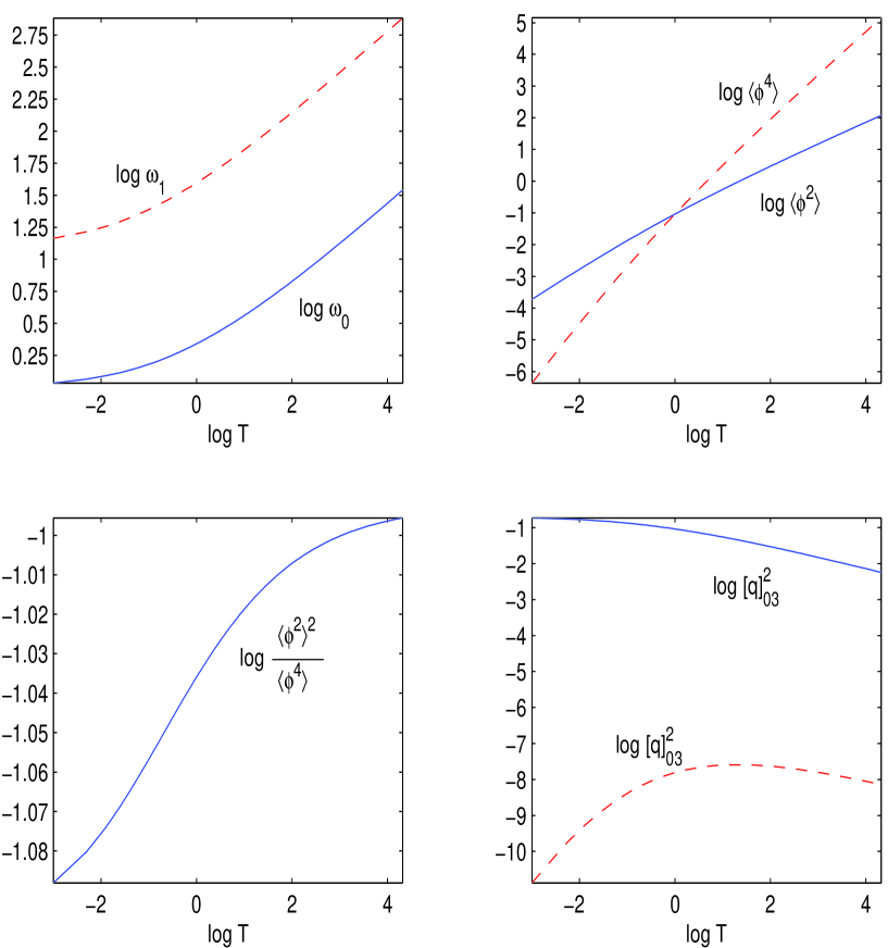
Figure 1: Log-log plot in the temperature of several quantities relevant for equilibrium observables.

II.9 Expected dynamical evolution

The exact results in the high temperature (large energy density) regime already suggest a preliminary picture for the dynamics in the case such that $Ta^{3}\ll 1$. In order to present this preliminary picture, it is convenient to summarize the main exact results valid in the high temperature limit (and $Ta^{3}\ll 1$).

$$\langle\pi^{2}\rangle=\frac{T}{2a}~{}~{},~{}~{}\langle\phi^{2}\rangle=0.45612\ldots T^{{2/3}}~{}~{},~{}~{}\langle\phi^{4}\rangle=0.56104\ldots T^{{4/3}}~{}~{},~{}~{}\frac{\langle\phi^{2}\rangle^{2}}{\langle\phi^{4}\rangle}=0.37077\ldots$$ (77)

$$\langle\pi^{2}\rangle=\frac{T}{2a}~{}~{},~{}~{}\langle\phi^{\prime 2}\rangle=\frac{T}{2a}\left[1-1.122\ldots(Ta^{3})^{1/3}\right]\simeq\frac{T}{2a}$$ (78)

$$\langle|\tilde{\pi}_{k}|^{2}\rangle=T~{}~{},~{}~{}\langle|\tilde{\phi}_{k}|^{2}\rangle=\frac{0.98880\ldots~{}T}{k^{2}+1.1818\ldots T^{2/3}}$$ (79)

where we have assumed $Ta^{3}\ll 1$ in eq.(78).

The important aspect gleaned from these exact results is that in equilibrium the nonlinear term is subdominant as compared to the space and temporal derivatives. Namely, while the harmonic spatial and temporal derivative terms $\langle\pi^{2}\rangle\sim\langle\phi^{\prime 2}\rangle\sim T/a\sim E/L$, the interaction term $\langle\phi^{4}\rangle\sim T^{{4/3}}$, hence $\langle\phi^{4}\rangle/\langle\pi^{2}\rangle\sim\langle\phi^{4}\rangle/\langle\phi^{\prime 2}\rangle\sim(Ta^{3})^{1/3}\ll 1$.

Consider solving the equation of motion (5) with initial conditions $\phi(x,t=0),\;\pi(x,t=0)$ so that the Fourier transform of $\phi,\pi$ have a power spectrum distributed on modes $k\ll\Lambda$. Since only small wavevectors are excited in the initial state, this entails that for large energy density $E/L\gg 1$ it has to be that $\phi^{4}\sim E/L\sim T/a$ and a large fraction of the energy density is initially stored in the interaction term but a very small fraction is in the derivative term $\phi^{\prime 2}$ since the initial power spectrum for $\phi^{\prime 2}$ is localized at small wavevectors. Thus initially, $\phi^{4}\gg\phi^{\prime 2}$. Since the time evolution conserves the energy, the interaction between modes can only transfer the energy. If the time evolution leads to a thermal equilibrium state, then after or near the equilibration time scale it must be that $\phi^{\prime 2}\gg\phi^{4}$ since in equilibrium the ensemble averages (which by the ergodic postulate are equivalent to time averages) are $\langle\phi^{4}\rangle/\langle\phi^{\prime 2}\rangle\sim(Ta^{3})^{1/3}\ll 1$.

The system will therefore evolve from the initial state to a final state of thermal equilibrium by transferring energy to modes of larger $k$, namely the initial power spectrum will necessarily broaden and energy will flow from the small $k$ values to larger values in order to increase $\phi^{\prime 2}$. Interaction energy will be then transferred to gradient energy via a cascade of energy towards larger $k$, namely an ultraviolet cascade. As an equilibrium state is reached the power spectrum of $\pi$, namely $|\tilde{\pi}_{k}|^{2}$ must become flat for all wavevectors up to the cutoff, since in equilibrium $\langle|\tilde{\pi}_{k}|^{2}\rangle=T$ [see eq.(40)]. Since initially the power spectrum has been prepared to be localized at small values of the momenta the flattening of the spectrum must be a direct consequence of the ultraviolet cascade, namely more and more wavevectors are being excited by the interaction. Interaction energy is transferred to spatio-temporal gradient energy at the expense of the interaction term becoming smaller. We envisage this cascade towards the ultraviolet as a front in wavector space at a value $\bar{k}(t)$ that moves towards the cutoff as time evolves. For $k\ll\bar{k}(t),\;|\tilde{\pi}_{k}|^{2}$ is approximately independent of $k$ and eventually must saturate at the value $T$ when the front $\bar{k}(t)$ reaches the cutoff.

As argued above, initially $\phi^{4}\gg\phi^{\prime 2}$ since the initial power spectrum for the field is concentrated at wavevectors well below $1/a$ and the energy density (conserved in the evolution) is $E/L\gg 1$. However if the evolution leads to thermal equilibrium interaction energy is transferred to gradient energy via the ultraviolet cascade as described above, resulting in that $\phi^{4}$ diminishes and $\phi^{\prime 2}$ increases with time. Therefore there is a time scale $t_{0}$ at which both terms are of the same order and the dynamics crosses over from being dominated by the interaction to being dominated by spatial derivatives. For $t\ll t_{0},\;\phi^{4}\gg\phi^{\prime 2}$ while for $t\gg t_{0},\;\phi^{4}\ll\phi^{\prime 2}$.

For $t\gg t_{0}$ the theory is weakly coupled since the interaction term is much smaller than $\phi^{\prime 2}$ and $\pi^{2}$, the ensuing dynamics becomes slower, the non-equilibrium dynamics during stage is probably well described in terms of kinetic equations, since the small interaction guarantees a separation of time scales.

These arguments that describe the expected dynamics are fairly robust and hinge upon very general features: i) energy conservation, ii) large energy density, iii) the initial condition determined by power spectra localized at small values of wavevectors, iv) the assumption that the dynamical evolution leads to a state of thermal equilibrium, v) the exact results obtained above in thermal equilibrium, which describe the final state of the dynamics.

A detailed numerical analysis of the evolution presented below confirms the robust features of these arguments (and more).

II.10 Criteria for thermalization

In the following section we undertake an exhaustive numerical study of the non-equilibrium evolution with the goal of understanding the dynamics that leads to thermalization and to assess the validity of the description presented above. We solve numerically the equation of motion (5) with given initial conditions. The initial conditions determine the energy density from which we can extract the equilibrium temperature either via eq.(65) in the low temperature limit $T\ll 1$ or via eq.(71) in the high temperature limit $T\gtrsim 1$. Since the classical field theory must always be understood with a fixed lattice (or UV) cutoff $2a$, the equilibrium temperature is obtained by providing the initial conditions, which fix the (conserved) energy density $E/L$ and the value of the cutoff $a$. Furthermore our primary interest is in studying the high temperature limit $T\gtrsim 1$, hence large energy density $E/L$, and will always work with values of the temperature and cutoff such that $Ta^{3}\ll 1$ in which case eq.(71) entails that the energy density $E/L\sim T/2a$.

In order to recognize when thermalization occurs we must define a consistent and stringent set of criteria. These are the following

• The ensemble averages should give the same result as the temporal averages over a macroscopically long time plus spatial volume averages. That is, we check the validity of ergodicity.

• The spatial (volume) and temporal average of $\pi^{2}(x,t)$ should approach the canonical ensemble average $\langle\pi^{2}\rangle=T/(2a)=E/L$.

• The spatial (volume) and temporal average of $\phi(x,t)~{},\;\phi^{2}(x,t),\;[\phi^{\prime}(x,t)]^{2},~{}[\dot{\phi}(x,t)]^{2}$ and $[\phi(x,t)]^{4}$ should approach their exact high temperature result eqs.(II.7)-(69) for high temperature and the behaviour plotted in figs. 1 for all temperatures.

• The spatial (volume) and temporal average of the canonical momentum correlator must tend to $T\delta(x-x^{\prime})$, which on the lattice would translate to $T/(2a)$ [see eqs.(39)-(40)].

• The temporal average of $|\tilde{\pi}_{k}(t)|^{2}$ (Fourier transform of the $\pi$-correlator) , which in equilibrium is given by $\langle|\tilde{\pi}_{k}|^{2}\rangle=T$. The temporal average of $|\tilde{\phi}_{k}(t)|^{2}$ (Fourier transform of the $\phi$-correlator) must reach their thermal values.

III Dynamics of thermalization.

Having provided an analysis of exact as well as approximate results of the cutoff classical field theory in equilibrium, we now pass on to the study of the dynamical evolution. In this section we study numerically the solution of the equation of motion (5) with different initial conditions, of a given large energy density. By changing the initial conditions for a fixed energy density we are studying the evolution of different members of a microcanonical ensemble on a fixed energy (density) shell.

Before embarking on the numerical study, we detail below our approach to solving the equations of motion by discretized dynamics in light–cone coordinates.

III.1 Discretized dynamics in light–cone coordinates

In order to solve numerically the evolution of the $\phi^{4}$ theory it is necessary to discretize space and time. We choose to do that on a light–cone latticecono . In this approach space and time are simultaneously discretized in light–cone coordinates with the same lattice spacing $a\sqrt{2}$, thus preserving as much as possible of the original relativistic invariance of the field equation

$${\ddot{\phi}}-\phi^{\prime\prime}+\phi+\phi^{3}=0\;.$$ (80)

Moreover, we choose a scheme where the discretized dynamics possesses an exactly conserved energy on the lattice.

Given a space–time field configuration $\phi(x,t)$, consider the two quantities

$$\begin{split}{\cal E}_{\pm}(x,t)=&\frac{1}{2a}\big{[}\phi(x+a,t)-\phi(x,t\pm a)\big{]}^{2}+\frac{1}{2a}\big{[}\phi(x-a,t)-\phi(x,t\pm a)\big{]}^{2}+\\ &+\frac{a}{4}\big{[}1+\phi^{2}(x,t\pm a)\big{]}\big{[}2+\phi^{2}(x+a,t)+\phi^{2}(x-a,t)\big{]}-\frac{a}{2}\;.\end{split}$$

In the limit $a\to 0$, assuming $\phi$ to be smooth enough, we obtain

$${\cal E}_{\pm}=a\left(\dot{\phi}^{2}+|\nabla\phi|^{2}+\phi^{2}+\tfrac{1}{2}\phi^{4}\right)+{\cal O}(a^{2})\;,$$

identifying the leading term in $a$ of both ${\cal E}_{+}$ and ${\cal E}_{-}$ with the energy density of the $\phi^{4}$ theory. However, to higher orders in $a$ they do differ; in fact

$${\cal E}_{+}(x,t)-{\cal E}_{-}(x,t)=\frac{\phi(x,t+a)-\phi(x,t-a)}{a}\;Q(x,t)\;,$$

where

$$Q(x,t)=\big{[}\phi(x,t+a)+\phi(x,t-a)\big{]}\Big{\{}1+\tfrac{a^{2}}{4}\big{[}2+\phi^{2}(x+a,t)+\phi^{2}(x-a,t)\big{]}\Big{\}}-\phi(x+a,t)-\phi(x-a,t)\;.$$

Hence, if $Q(x,t)=0$, then ${\cal E}_{+}(x,t)={\cal E}_{-}(x,t)$ also on the lattice. In this case the total lattice energy

$$E=\sum_{n}{\cal E}_{+}(2n\,a,t)$$ (81)

is exactly conserved in time, since it can also be written

$$E=\sum_{n}{\cal E}_{-}(2n\,a+a,t+a)\;.$$ (82)

This holds exactly on infinite space. If space is restricted to the segment $[0,L]$, suitable boundary conditions on $\phi(x,t)$ are necessary; PBC are of this type if $L=2Na$ with $N$ an integer.

In conclusion, we may regard $Q(x,t)=0$ as a discrete field equation which conserves the total energy $E$. More explicitly, $Q(x,t)=0$ can be written as the recursion rule

$$\phi(x,t+a)=-\phi(x,t-a)+\frac{\phi(x+a,t)+\phi(x-a,t)}{1+\tfrac{a^{2}}{4}\big{[}2+\phi^{2}(x+a,t)+\phi^{2}(x-a,t)\big{]}}$$ (83)

which evidently allows to propagate in time any configuration known in a time interval of width $a$.

It is easy to check that $Q(x,t)=0$ indeed becomes eq.(80) in the continuum $a\to 0$ limit. The order $a^{0}$ is trivially satisfied, odd powers of $a$ vanish identically as a consequence of the symmetry of eq.(83) under $a\to-a$, while the order $a^{2}$ produces eq.(80).

Keeping up to $\mathcal{O}(a^{4})$ in eq.(83) yields,

$${\ddot{\phi}}-\phi^{\prime\prime}+\phi+\phi^{3}=a^{2}\left\{-\frac{1}{2}\left[\phi^{\prime\prime}-\phi-\phi^{3}\right](1+\phi^{2})+\frac{1}{12}(\phi^{\prime\prime\prime\prime}-{\ddddot{\phi}})-\;\phi(\phi^{\prime 2}+\phi\;\phi^{\prime\prime})\right\}+{\cal O}(a^{4})\;.$$ (84)

To cast eq.(83) in a form suitable for numerical simulations, we define the lattice fields $F(n,s)$ and $G(n,s)$ as

$$F(n,s)\equiv\phi(2n\,a,2s\,a)\;,\quad G(n,s)\equiv\phi([2n-1]\,a,[2s+1]\,a)\;,\quad n,s\in{\mathbb{Z}}\;.$$

We then obtain the iterative system

$$F(n,s+1)=-F(n,s)+\frac{G(n,s)+G(n+1,s)}{1+\frac{a^{2}}{4}\left[2+G^{2}(n,s)+G^{2}(n+1,s)\right]}$$ (85)

(86)

$$G(n,s+1)=-G(n,s)+\frac{F(n-1,s+1)+F(n,s+1)}{1+\frac{a^{2}}{4}\left[2+F^{2}(n-1,s+1)+F^{2}(n,s+1)\right]}\;.$$ (87)

with the PBC $F(n+N,s)=F(n,s)$ and $G(n+N,s)=G(n,s)$. As initial conditions we have to specify $F(n,0)$ and $G(n,0)$ for $0\leq n\leq N-1$. Once these values of the fields are specified, the iteration rules (85) uniquely define $F(n,s)$ and $G(n,s)$ for all $s\neq 0$. A comparison of this discretized dynamics with other more traditional numerical treatments of hyperbolic partial differential equations was performed in zanlungo . Here we only notice that this approach is particularly efficient, stable and accurate, specially when the continuum limit $a\to 0$ and very long evolution times are of interest.

All observables of the continuum are rewritten on the lattice in terms of the basic fields $F(n,s)$ and $G(n,s)$. In particular, time and space derivatives are replaced by finite diferences. We always choose symmetric discretization rules such that lattice observables differ from their continuum limit by ${\cal O}(a^{2})$. In the sequel, while referring to properly discretized observables, we shall keep using the continuum notation for simplicity,

III.2 Initial Conditions

We studied a variety of initial conditions with a fixed energy density in our calculations. In these studies the power is concentrated in the infrared; that is, $|{\tilde{\phi}}_{k}(0)|^{2}$ and $|{\tilde{\pi}}_{k}(0)|^{2}$ are large for wavenumbers well below the cutoff $\Lambda=\frac{\pi}{2a}$. We considered the following sets of initial conditions:

• Superpositions of plane waves: The initial fields have the form

  $$\phi(x,0)=A\sum_{i}c_{i}\;\cos(k_{i}\,x+2\,\pi\,\gamma_{i})\quad,\quad\pi(x,0)=A\sum_{i}d_{i}\;\cos(k_{i}\,x+2\,\pi\,\delta_{i})\;.$$ (88)

  The wavenumbers $k_{i}=2\pi n_{i}/L$ are chosen in the interval $[0,k_{\rm max}]$ with $k_{\rm max}=50\pi/L=25\pi/(N\,a)\ll\pi/(2a)$. We will refer to these initial conditions as hard because these plane waves have sharp values for the wavenumbers. The power spectra $|\tilde{\phi}_{k}|^{2}~{};~{}|\tilde{\pi}_{k}|^{2}$ are sharply peaked at discrete (and small ) values of the momenta small compared with the cutoff $\Lambda=\frac{\pi}{2a}$.

• Superpositions of localized wave packets: These are configurations of the form

  $$\phi(x,0)=A\sum_{i}c_{i}\;w(x-x_{i})\quad,\quad\pi(x,0)=A\sum_{i}d_{i}\;w(x-y_{i})\;.$$ (89)

  where we enforce the PBC by choosing,

  $$w(x)=\sum_{n\in{\mathbb{Z}}}w_{0}(k_{max}[x-n\,L])$$

  with $w_{0}(x)$ either the gaussian, $w_{0}(x)=e^{-x^{2}}$, or the lorentzian, $w_{0}(x)=\frac{1}{1+x^{2}}$. In practice, with our choice $L\sim 20$, only few terms in the sum are needed. These fields have support throughout Fourier space, but peaked as gaussians or simple exponentials at low wavenumbers $k\lesssim k_{\rm max}$. We will refer to these initial conditions as soft since these correspond to continuous and slowly varying power spectra.

• Random on a fixed energy shell: A systematic way to decrease fluctuations is to average over initial conditions corresponding to a given value of the total energy. A microcanonical description gives equal a priori probability to all the configurations on the same energy shell.

  Thus, we choose smooth initial conditions as defined by eqs.(88)-(89) and we average over them with unit weight choosing random values for the various coefficients. That is, we choose in eq.(88) the wavenumbers $k_{i}=2\pi n_{i}/L$ at random both in number and in location, within the interval $[0,k_{\rm max}]$ with $k_{\rm max}=50\pi/L=25\pi/(N\,a)\ll\pi/(2a)$. The positions $x_{i}\,,y_{i}$ in eq.(89) are chosen at random in $[0,L]$. The phases in eq.(88), $\gamma_{i}\,,\delta_{i}$, and the relative amplitudes $c_{i}\,,d_{i}$ are also chosen at random in the interval $[0,1]$. Finally, for any given realization of $k_{i}\,,\gamma_{i}\,,\delta_{i}\,,c_{i}\,,d_{i}$, the overall amplitude $A$ is fixed through the energy density $E/L$ so all the configurations chosen are on the same energy shell.

  Typically, we performed averages over 30 initial conditions.

For a fixed energy (density) the overall amplitude $A$ in eqs.(88) and (89) is fixed for any choice of $c_{i},\,d_{i},\,\gamma_{i},\,\delta_{i}$ by the requirement that the initial configurations had always the same energy $E$. We considered several values of the energy density $E/L$ ranging from $2.6$ to $\sim 10^{4}$.

We notice also that all our initial configurations have vanishing total momentum $\int dx\,\pi\phi^{\prime}$, which is a conserved quantity for PBC.

III.3 Averaged observables

The key observables in our investigation are the basic quantities

$$\phi,\,\phi^{2},\,\phi^{4},\,{\dot{\phi}}^{2},\,{\phi^{\prime}}^{2}\;,$$ (90)

as well as the power spectra of $\phi$ and $\pi$, that is $|{\tilde{\phi}}_{k}(t)|^{2}$ and $|{\tilde{\pi}}_{k}(t)|^{2}$, where,

$${\tilde{\phi}}_{k}(t)\equiv\int_{0}^{L}\frac{dx}{\sqrt{L}}\;e^{ikx}\;\phi(x,t)\quad,\quad{\tilde{\pi}}_{k}(t)\equiv\int_{0}^{L}\frac{dx}{\sqrt{L}}\;e^{ikx}\;\pi(x,t)\;,$$

as in eq.(6).

In referencewett the correlation function of the canonical momenta was studied which is particularly important since in equilibrium in the classical theory it is Gaussian. We here study a large number of independent observables and correlation functions since the criteria established above for thermalization based on the exact results apply to many different correlation functions.

In accordance with the anticipation at the end of sec. III.1, we are using here the continuum notation also for the Fourier transforms, although they actually are discrete Fourier transforms.

The fluctuations of all these observables do not vanish upon time evolution. Hence for generic initial conditions they do not have a limit as $t\to\infty$. These are fine–grained or microscopic observables. Typically there are several spatio-temporal scales, the microscopic scales correspond to very fast oscillations and short distance variations that are of no relevance to a thermodynamic description. We are interested in longer, macroscopic scales that describe the relaxation of observables towards a state of equilibrium.

In particular the ergodic postulate states that ensemble averages must be identified with long time averages as well as spatial averages over macroscopic-sized regions.

To make contact between the time evolution and the thermal averages we need to properly average the microscopic fluctuations.

First of all, for local quantities such as those in eq.(90) we take the spatial average. Secondly, we take suitable time averages of all key observables in the following way

$$\overline{\phi^{2}}(t)\equiv\frac{1}{\tau}\int_{t-\tau}^{t}dt^{\prime}\;\;\frac{1}{L}\;\int_{0}^{L}dx\,[\phi(x,t^{\prime})]^{2}\;.$$ (91)

where $\tau\gg a$ stands for the length of the time interval where we average. We find that the period of the fast (microscopic oscillations) themselves vary in time suggesting a sliding averaging in which $\tau$ grows in time to compensate for the growth in the period of the fast time variation. We find that a practical and efficient manner to implement this averaging is to use

$$\tau(t)=\tau(0)+C\;t$$ (92)

where $\tau(0);C$ small and positive with typical values $\sim 0.1$. In this way $t\gg\tau(t)$ and the dependence on the initial values becomes negligible for practically accessible times. This method is quite effective in revealing general features of the (logarithmic) time evolution such as the presence of distinct stages characterized by well separated macroscopic time scales.

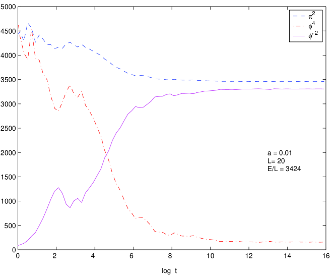
Figure 2: ${\overline{\phi^{\prime 2}}}(t),\;{\overline{\phi^{4}}}(t)$ and ${\overline{\pi^{2}}}(t)$ as a function of the logarithm of the physical time for $E/L=3424,\;L=20$ and $a=0.01$.

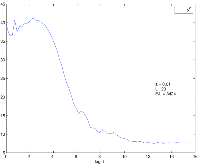
Figure 3: ${\overline{\phi^{2}}}(t)$ as a function of the logarithm of time for $T=69.2,\;E/L=3424,\;L=20$ and $a=0.01$.

Altogether, we denote the results of all coarse-grainings simply with an overbar (not to be confused with the complete time average of section II.4) to avoid cluttering of notation. For example we have in the case of random initial conditions on the energy shell

$$\overline{\phi^{4}}(t)=\frac{1}{M}\sum_{i=1}^{M}\;\frac{1}{\tau}\;\int_{t-\tau}^{t}dt^{\prime}\;\frac{1}{L}\;\int_{0}^{L}dx\;[\phi^{(i)}(x,t^{\prime})]^{4}\;.$$

where the superscript ⁽ⁱ⁾ labels the $M$ different choices of smooth initial conditions, all with the same energy density $E/L$, we have taken $M\sim 30$ in our study. Likewise,

$$\overline{|{\tilde{\pi}}_{k}|^{2}}(t)=\frac{1}{M}\sum_{i=1}^{M}\;\frac{1}{\tau}\;\int_{t-\tau}^{t}dt^{\prime}\;|{\tilde{\pi}^{(i)}}_{k}(t^{\prime})|^{2}$$ (93)

where we used the reality condition ${\tilde{\pi}}_{k}={\tilde{\pi}}_{-k}^{\,\ast}$. Analogous expressions hold for $\phi,\;\phi^{2},\;\phi^{4},\;\pi^{2},\;\phi^{\prime 2}$ and $|{\tilde{\phi}}_{k}|^{2}$.

In particular, due to the linearity of these averages, we have the sum rules:

$$\int_{-\Lambda}^{+\Lambda}\frac{dk}{2\pi}\;\overline{|{\tilde{\phi}}_{k}|^{2}}(t)=\overline{\phi^{2}}(t)\quad,\quad\int_{-\Lambda}^{+\Lambda}\frac{dk}{2\pi}\;\overline{|{\tilde{\pi}}_{k}|^{2}}(t)=\overline{\pi^{2}}(t)\quad,\quad\int_{-\Lambda}^{+\Lambda}\frac{dk}{2\pi}\;k^{2}\;\overline{|{\tilde{\phi}}_{k}|^{2}}(t)=\overline{\phi^{\prime 2}}(t)\;.$$ (94)

Where UV cutoff in the light–cone lattice is $\Lambda=\pi/(2a)$.

The power spectra $\overline{|{\tilde{\phi}_{k}}|^{2}}(t)$ and $\overline{|{\tilde{\pi}_{k}}|^{2}}(t)$ are connected to equal–time correlation functions of $\phi(x,t)$ and $\pi(x,t)$, respectively, just as it happens at thermal equilibrium [see e.g. eq.(53)]. We have, for instance

$$\begin{split}\overline{|{\tilde{\phi}_{k}}|^{2}}(t)&=\int_{0}^{L}dx\;e^{-ikx}\;\overline{\phi\phi}(x,t)\;,\\ \overline{\phi\phi}(x,t)&=\frac{1}{M}\sum_{i=1}^{M}\frac{1}{\tau}\int_{t-\tau}^{t}dt^{\prime}\;\frac{1}{L}\int_{0}^{L}dy\;\phi^{(i)}(y,t^{\prime})\;\phi^{(i)}(x+y,t^{\prime})\;.\end{split}$$ (95)

with similar relations between $\overline{|{\tilde{\pi}_{k}}|^{2}}(t)$ and or $\overline{\pi\pi}(x,t)$ and between $k^{2}\overline{|{\tilde{\phi}_{k}}|^{2}}(t)$ and $\overline{\phi^{\prime}\phi^{\prime}}(x,t)$.

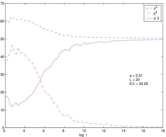
Figure 4: ${\overline{\phi^{\prime 2}}}(t),\;{\overline{\phi^{4}}}(t)$ and ${\overline{\pi^{2}}}(t)$ as a function of the logarithm of the physical time for $E/L=50.28,\;L=20$ and $a=0.01$.

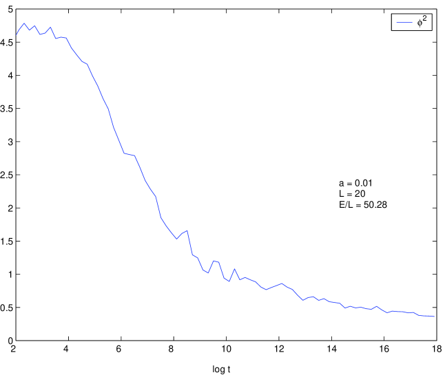
Figure 5: ${\overline{\phi^{2}}}(t)$ as a function of the logarithm of time for $E/L=50.28,\;L=20$ and $a=0.01$.

It is useful to define the normalized power spectrum of $\pi$,

$$P(k,t)\equiv\frac{\overline{|{\tilde{\pi}}_{k}|^{2}}(t)}{\overline{\pi^{2}}(t)}\;,$$ (96)

which describes the distribution of power over the wavenumbers, it is normalized so that,

$$\int_{-\Lambda}^{+\Lambda}\frac{dk}{2\pi}\;P(k,t)=1$$ (97)

Another important quantity of paramount importance to describe the cascade described in section II.9 above is the average wavenumber

$$\overline{k}(t)=\int^{+\Lambda}_{-\Lambda}\frac{dk}{2\pi}\;|k|\;P(k,t)\;.$$ (98)

In thermal equilibrium $\langle|\tilde{\pi}_{k}|^{2}\rangle=T$, $\langle\pi^{2}\rangle=T/(2a)=T\Lambda/\pi$, therefore in equilibrium $\overline{k}_{eq}=\Lambda/2$.

The physical significance of this quantity becomes obvious by considering the situation in which the power spectrum $|\tilde{\pi}_{k}|^{2}$ is approximately flat in a region of wavevectors $|k|\leq k_{M}$ and negligible elsewhere, namely $|\tilde{\pi}_{k}|^{2}\propto\Theta(k^{2}_{M}-k^{2})$. In this case $\overline{k}(t)\equiv\frac{k_{M}}{2}$. The relevance of this effective quantity will become clear below when we study in detail the process of cascade of energy towards the UV, described in section II.9, where it will become clear that $2\overline{k}(t)$ determines the front of the ultraviolet cascade as described in section II.9.

To summarize, we perform spatio-temporal averages in the isolated system with fixed energy (density) which is equivalent to microcanonical ensemble averages at long time by the ergodic postulate. In the thermodynamic limit, it is expected that microcanonical and canonical ensembles will yield the same equilibrium results provided the equilibrium temperature $T$ is identified with the energy density as per eqs.(65) or (71) in the low or high temperature limit respectively.

While in refs. wett and zanlungo only the variance of $\pi^{2}$ was studied as a measure of gaussianity and thermalization, we study many different correlators, since as described above the exact solution in thermal equilibrium furnishes a stringent set of criteria for thermalization.

III.4 Time evolution of basic observables

We use the lattice field equations, eq.(85), to evolve the initial configurations in time and compute the time and space average of the basic quantities (90) as a function of time for $10<t<10^{8}$ and $0.1<a<0.0001$.

We confirmed that the lattice energy eqs.(81)-(82) is indeed conserved with large accuracy.

Figs. 2, 3, display ${\overline{{\phi^{\prime}}^{2}}}(t),\;{\overline{\phi^{4}}}(t),\;{\overline{\pi^{2}}}(t)$ and ${{\overline{\phi^{2}}}}(t)$, respectively, as functions of time for $E/L=3424,\;L=20$ and $a=0.01$ corresponding to an equilibrium temperature $T\sim 68.5$. Figs. 4 and 5, display the same quantities as functions of time for $E/L=50.28,\;L=20$ and $a=0.01$

In figs. 2-5 the initial conditions are the plane waves eq.(88) with parameters that fix $\pi^{2}\sim\phi^{4}\sim E/L$ initially. No average over initial conditions is performed and we used the sliding time average with linearly growing time intervals as in eq.(92).

These figures clearly reveal the expected dynamics as described in section II.9 above. Initially $\bar{\phi^{\prime 2}}(t)$ is small reflecting the fact that the initial conditions determine a power spectrum localized at wavectors $k\ll 1/a$. The mode mixing entailed by the interaction is transferring power to larger wavevectors, thus effectively transferring energy from the interaction term, which diminishes, to the spatial gradient term which increases. As is clear from these figures, all magnitudes tend to a limit for late times. The late time limits are the thermal equilibrium values, as we discuss below in detail,

The growth of ${\overline{{\phi^{\prime}}^{2}}}(t)$ at the expense of the interaction term ${\overline{\phi^{4}}}(t)$ shows that thermalization is a result of the flow of energy towards larger $k$ modes, namely the ultraviolet cascade ultimately leads to the thermal equilibrium state.

We find three distinct stages of evolution for a wide choice of initial conditions.

• A first stage with relatively important fluctuations and whose precise structure depends on the initial conditions. Such stage can be seen in figs. 2-5 for $\ln t<5$, that is $t<200$. The value $t_{i}\sim 200$ turns to be independent of both $a$ and $E/L$ as long $E/L$ is not very small. Namely, we find $t_{i}\sim 200$ for $0.1>a>0.0002$ and $E/L\gtrsim 10$. For lower values of $E/L,\;t_{i}$ increases sharply as shown in figs. 6 and 25. In addition, for such low values of $E/L,\;t_{i}$ becomes dependent on the details of the initial conditions but is not relevant for our study which focused on the high density case. During this first stage the transfer of energies via the cascade begins to be operative and becomes most effective at the time scale $t_{i}$. We see that $t_{i}$ can be identified with the time scale at which the interaction and gradient terms are of the same order and the crossover from a strongly interacting $\phi^{4}\gg\phi^{\prime 2}$ to a weakly interacting theory occurs. Thus the first stage corresponds to $t\leq t_{i}\sim 200$ during which the cascade is the result of large interaction energy which is redistributed to larger wavevectors via mode mixing and the dynamics is dominated by the interaction.

• There is a second stage where ${\overline{{\phi^{\prime}}^{2}}}(t),\;{\overline{{\dot{\phi}}^{2}}}(t),\;{\overline{\phi^{2}}}(t)$ and ${\overline{\phi^{4}}}(t)$ are about the same order $\sim E/L$. During this stage there is a crossover from a strongly to a weakly interacting theory since at the end of this second stage the spatio-temporal gradient terms are much larger than the non-linear term. During this second stage the cascade is very efficient in redistributing the energy.

  In figs. 2-5 this second stage corresponds to $5<\ln t<10$ for $a=0.01$.

  We find that the behaviour of the observables during this second transient stage depends to some extent on the initial conditions. For hard initial conditions [as eq.(88)] we find much steeper curves for ${\overline{{\phi^{\prime}}^{2}}}(t),\;{\overline{{\dot{\phi}}^{2}}}(t),\;{\overline{\phi^{2}}}(t)$ and ${\overline{\phi^{4}}}(t)$ than for soft initial conditions [as eqs.(89)]. Thus this second stage corresponds to an interval after the time at which the spatial gradient and interaction terms cross.

  While the details of the dynamics during this stage depend on the initial conditions, the presence of this stage during a time interval $5\lesssim\ln t\lesssim 10\sim\ln t_{0}$ is fairly robust. We found such intermediate stage for all types of initial conditions, and a wide range of lattice spacings and energy density.

  During this second stage $\overline{\pi^{2}}(t)$ varies with time more slowly than ${\overline{{\phi^{\prime}}^{2}}}(t),\;{\overline{\phi^{2}}}(t)$ and ${\overline{\phi^{4}}}(t)$.

• After this transient second stage there is a third stage where these physical quantities approach their thermal equilibrium values. The third stage starts at a time scale $t_{0}\sim 50000$. The value of $t_{0}$ turns to be independent of both $a$ and $E/L$ as long $E/L$ is not very small. That is, for $E/L\gtrsim 10$.

  In particular, ${\overline{\pi^{2}}(t)}$ slowly decreases to its asymptotic value which agrees with the thermal equilibrium value $T/(2a)$, that is, using eq.(65):

  $$\lim_{t\to\infty}\overline{\pi^{2}}(t)=\frac{T}{2a}=\frac{E}{L}+{\cal O}(a^{2})\;.$$ (99)

  The dynamics during this third stage is also driven by the ultraviolet cascade but unlike the earlier two stages wherein the details depend on the initial conditions, we find that this third stage is described by a universal cascade independent of the initial conditions as we shall see in the next section. In particular, the results obtained during the third stage for sharp initial conditions [eq.(88)] are independent of the chosen wavenumbres $k_{i}$ provided they do not approach the lattice cutoff. The third stage ends at a time $\sim t_{1}$ when the lattice size effects start to play a role. For the cases depicted in figs. 2-3 and figs. 4-5 we have $\ln t_{1}\sim 12$ and $\ln t_{1}\sim 17$, respectively.

• The fourth and final stage extends for times beyond $t_{1}$. Thermalization is reached here, strictly speaking, only for infinite times. Since the dynamics feels here the details of the discretization adopted, we shall not study this stage in detail.

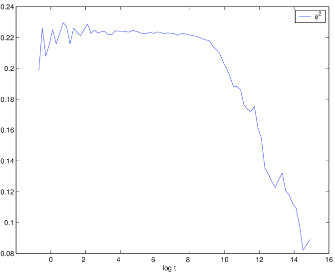
Figure 6: ${\overline{\phi^{2}}}(t)$ as a function of the logarithm of the time $t$ for $E/L=3.67,\;L=20$ and $a=0.01$. For such a low value of $E/L$ the cascade starts much later for $\log t_{0}\sim 17$

Figs. 7-8 display ${\overline{\phi}}(t)$ and $\log|{\overline{\phi}}(t)|$ as a function of the logarithm of the time for $E/L=3424$ and $E/L=50.28$ for $L=20$ and $a=0.01$, respectively.

We see that the relaxation of $\phi$ towards its thermal equilibrium value ($\phi=0$) is different from the other physical quantities previously discussed. This is due to the fact that the vanishing of ${\overline{\phi}}$ is connected to a symmetry of the model. We find that ${\overline{\phi}}(t)$ relaxes as $1/t$ for $t\lesssim t_{0}$ (during the first two stages of thermalization) and as $\sim 1/\sqrt{t}$ for $t\gtrsim t_{0}$ (during the two subsequent stages).

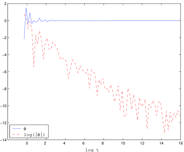
Figure 7: ${\overline{\phi}}(t)$ and $\log|{\overline{\phi}}(t)|$ as a function of the logarithm of the time $t$ for $E/L=3424,\;L=20$ and $a=0.01$.

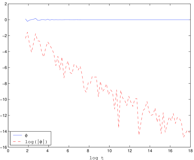
Figure 8: ${\overline{\phi}}(t)$ and $\log|{\overline{\phi}}(t)|$ as a function of the logarithm of the time $t$ for $E/L=50.28,\;L=20$ and $a=0.01$.

III.5 Time Evolution of the Correlation Functions

We now turn our attention to the study of correlation functions.

According to the Fourier transform relationship eq.(95) between the power spectrum $\overline{|{\tilde{\phi}}|^{2}}(k,t)$ and the equal–time correlation function $\overline{\phi\phi}(x,t)$, there are two approaches to the numerical evolution of such quantities (we specialize here on $\phi$ but the discussions applies equally well to $\pi$). We extract the field $\phi(x,t)$ from the lattice fields $F(n,s)$ and $G(n,s)$, Fourier–transform it to ${\tilde{\phi}}_{k}(t)$ and then perform all needed averages on $|{\tilde{\phi}}_{k}(t)|^{2}$. Or we directly compute averages of the correlations of $F(n,s)$ and $G(n,s)$ and extract from them the correlations $\overline{\phi\phi}(x,t)$ and $\overline{\pi\pi}(x,t)$. We found that both methods yield the same numerical results (see Appendix).

Moreover, when using the approach with growing time averages as in eq.(92) with a unique initial condition, one realizes that the simply time–averaged correlation

$$\frac{1}{\tau}\;\int_{t-\tau}^{t}dt^{\prime}\;\phi(x,t^{\prime})\;\phi(x^{\prime},t^{\prime})\;.$$ (100)

very soon (in the logarithm of time) becomes translation invariant, that is a function only on the distance $|x-x^{\prime}|$, making the time consuming space average unnecessary.

We plot in figs. 9, 10 and 11 thee example of the typical profiles of $\overline{\phi\phi}(x,t)$, $k^{2}\,\overline{|{\tilde{\phi}}_{k}|^{2}}(t)$ and $\overline{|{\tilde{\pi}}_{k}|^{2}}(t)$, respectively, for one given choice of parameters. We see from fig 9. that the angle point at $x=0$, characteristic of the equilibrium correlation function $G(x)$ [see eqs.(35) and (55)] is developping. This appears more evident in Fourier space, fig 10, since the region where $k^{2}\,\overline{|{\tilde{\phi}}_{k}|^{2}}(t)$ is large and almost constant is spreading towards the UV cutoff. Likewise we see the same UV cascade for $\overline{|{\tilde{\pi}}_{k}|^{2}}(t)$ in fig 11. The power spectrum of the canonical momentum $\pi$ will be discussed in detail in the next section.

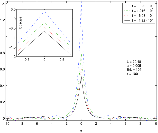
Figure 9: The correlation $\overline{\phi\phi}(x,t)$ as a function of $x$ at four different times. It takes the thermal form eq.(73) for an effective temperature $T_{\rm eff}(t)$.

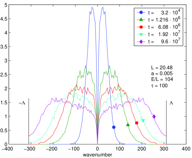
Figure 10: $k^{2}\overline{|{\tilde{\phi}_{k}}|^{2}}(t)$ vs. $k$ at the same times of fig. 9. It is described in the central plateau by the thermal spectrum eq.(73) for an effective temperature $T_{\rm eff}(t)$. $T_{\rm eff}(t)$ can be read here approximately from the height of the plateau.

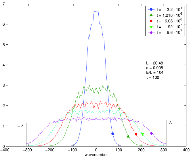
Figure 11: $\overline{|{\tilde{\pi}_{k}}|^{2}}(t)$ vs. $k$ at the same times of figs. 9 and 10. It is described in the central plateau by the flat thermal spectrum eq.(59)for an effective temperature $T_{\rm eff}(t)$. The height of the plateau is identical to fig.10 as expected.

Figure 12: Virialization: the logarithm of $\frac{L^{2}}{E^{2}\;a^{3}}\times|\Delta(t)|$ vs. the logarithm of the time for $E/L=50.3,\;728$ and $3424$ with $a=0.01$ and for $E/L=34861$ with $a=0.001$.

III.6 Early Virialization

We depict in fig. 12 the quantity,

$$\Delta(t)\equiv\langle\dot{\phi}^{2}\rangle(t)-\langle\phi^{\prime 2}\rangle(t)-\langle\phi^{2}\rangle(t)-\langle\phi^{4}\rangle(t)\;.$$

This quantity vanishes when the virial theorem is fulfilled [see eq.(48)]. It turns out to be negative for finite times and nonzero $a$. We see from fig. 12 that $|\Delta(t)|$ starts to decrease at times earlier than $t_{0}$. Therefore, the model starts to virialize before it starts to thermalize. $|\Delta(t)|$ keeps decreasing with time and tends to a nonzero value which is of the order ${\cal O}(a^{3})$ for $t\to\infty$. This is to be expected since eq.(48) only holds in the continuum limit and receives corrections in the lattice.

IV The Energy Cascade

We describe here the flow of energy towards higher frequencies leading towards thermalization. Such cascade turns to be universal (independent of the lattice spacing and of $E/L$) and exhibits scaling properties within a wide range of time.

IV.1 Power spectrum of $\pi$ and the universal cascade

The chosen initial conditions eqs.(88)–(89) are such that the power is concentrated in long wavelength modes $k$ well below the ultraviolet cutoff $\Lambda=\pi/(2a)$. Therefore, $\overline{|{\tilde{\pi}_{k}}|^{2}}(0)\,;\,\overline{|{\tilde{\phi}_{k}}|^{2}}(0)$ are concentrated on small $k$. During the time evolution the non-linearity gradually transfers energy off to higher $k-$modes leading to the ultraviolet cascade as discussed above.

The typical behaviour of $\overline{|{\tilde{\pi}_{k}}|^{2}}(t)$ is shown in figs. 13, 14 and 15. In these figures we have averaged over time with constant intervals $\tau$, and on the initial conditions as defined by eq.(93). This plots have also been smoothed by a moving average over wavenumbers with averaging intervals of size $32\pi/L$ [see the Appendix for details].

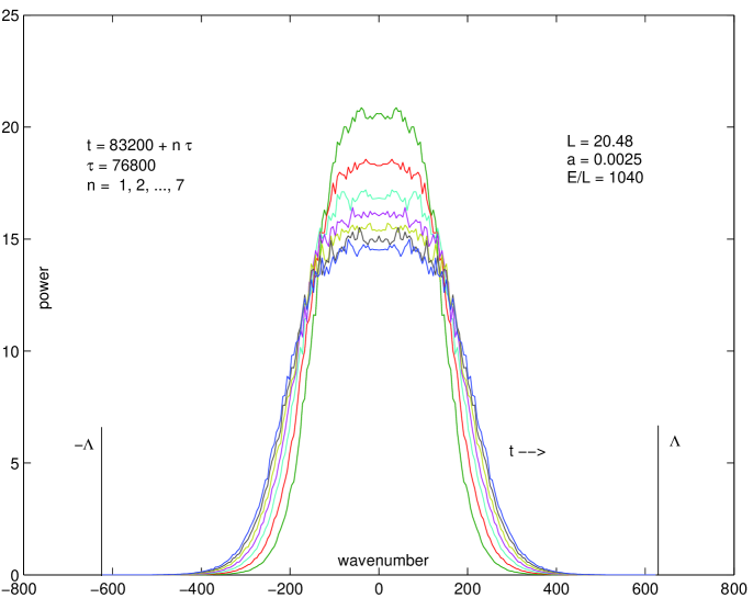
Figure 13: $\overline{|{\tilde{\pi}_{k}}|^{2}}(t)$ cascade still far from the UV cutoff.

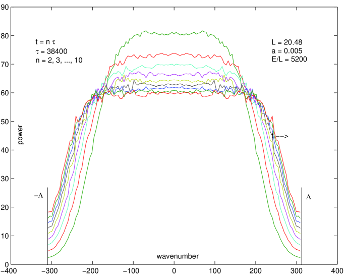
Figure 14: $\overline{|{\tilde{\pi}_{k}}|^{2}}(t)$ cascade reaching the UV cutoff.

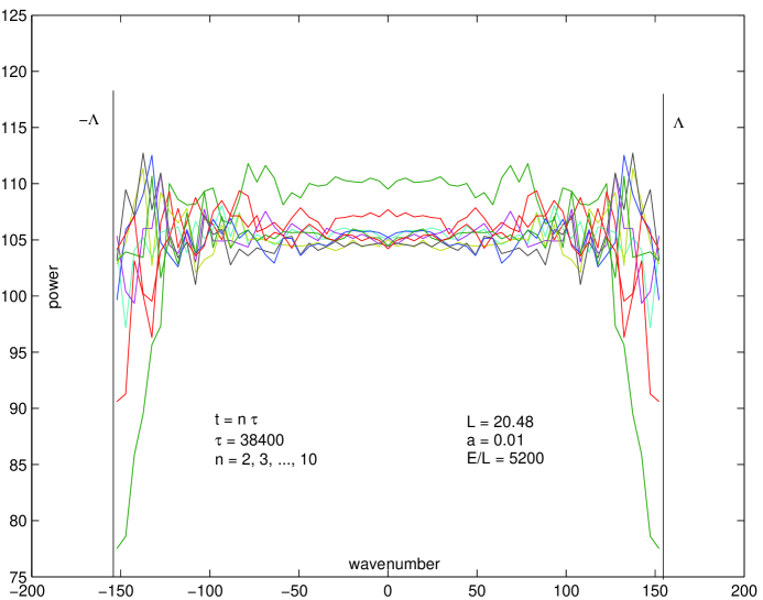
Figure 15: $\overline{|{\tilde{\pi}_{k}}|^{2}}(t)$ cascade close to complete thermalization.

The time evolution of the power spectrum $\overline{|{\tilde{\pi}_{k}}|^{2}}(t)$ features the ultraviolet cascade in a very clear manner. The gradual transfer of energy to larger wavevectors results in a the formation of a central plateau which spreads over higher wavenumbers as time grows decreasing its height. This plateau ends abruptly at a value of the wavector which determines the front of the cascade. From the definition of $\overline{k}(t)$ given by eq.(98) and the discussion that follows it, it is clear that this cascade front is given by $2\;\overline{k}(t)$.

The limiting form of $\overline{|{\tilde{\pi}_{k}}|^{2}}(t)$ for $t\to\infty$ is flat, as expected from thermal equilibrium, eq.(59) [see fig. 15]:

$$\lim_{t\to\infty}\overline{|{\tilde{\pi}_{k}}|^{2}}(t)=T\;.$$ (101)

The second and third stages described in sec. III.D for $t\gg t_{0}$ correspond to the steady flow of energy towards higher wavenumbers with a steady increase of the average wavenumber $\overline{k}(t)$ towards its asymptotic value of thermal equilibrium [see figs. 16] and decrease of the height of the plateau. Thus the front of the cascade $2\;\overline{k}(t)$ advances towards its limiting value, given by the cutoff $2\;\overline{k}(\infty)=\Lambda=\frac{\pi}{2a}$ leaving behind a wake in local thermal equilibrium at a temperature $T_{\rm eff}(t)$ corresponding to the height of the plateau.

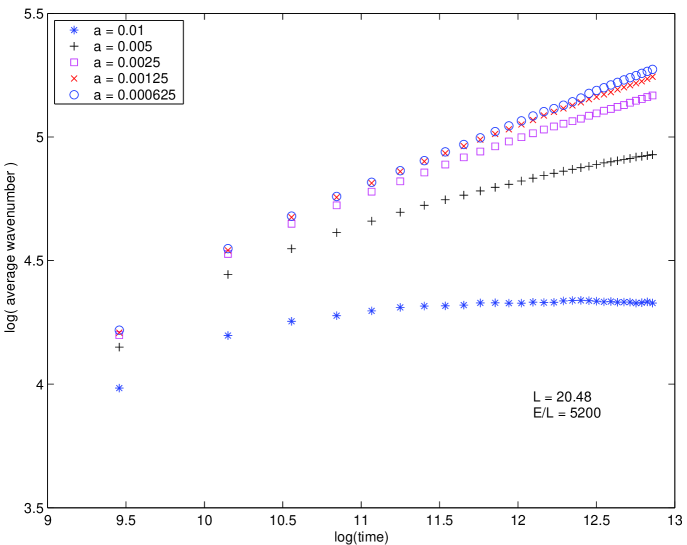
Figure 16: Numerical evaluation of the average wavenumber $\overline{k}(t)$ for different values of the UV cutoff, at fixed energy density. When $a=0.01$ the system almost thermalizes [see fig. 15] and $\overline{k}(t)$ saturates to its equilibrium value $\Lambda/2$. When $a=0.005$ the bulk of the cascade reaches the UV cutoff, causing a significant bending. For smaller $a$ the bulk of the cascade is still far away from the cutoff at the times depicted here.

Figs. 13-15 clearly show that there are only two relevant wavevector scales in the power spectrum $\overline{|{\tilde{\pi}_{k}}|^{2}}(t)$: the front of the cascade $2\;\overline{k}(t)$ and the momentum cutoff $\Lambda$. Neglecting fluctuations in the plateau, it is clear from these figures that for $k\lesssim 2\;\overline{k}(t)$ the power spectrum is flat just as in the equilibrium case, and for $2\;\overline{k}(t)\ll\Lambda$ the shape of the power spectrum is very simple and insensitive to the cutoff.

We therefore reexpress the distribution $P(k,t)$ defined by eq.(96) in terms of dimensionless ratios as follows,

$$P(k,t)=\frac{1}{\overline{k}(t)}\,F(u,v)\;,\quad u\equiv\frac{k}{\overline{k}(t)}\;,\quad v(t)\equiv\frac{2\,\overline{k}(t)}{\Lambda}=\frac{4}{\pi}\;\overline{k}(t)\;a\;.$$ (102)

with the asymptotic behavior of $v(t)$ given by

$$v(t)\buildrel t\rightarrow\infty\over{=}1$$

Our numerical analysis shows that during a fairly large time interval $t_{1}\gg t\gg t_{0}$, during which $2\;\overline{k}(t)\ll\Lambda$, the shape function $F(u,v)$ becomes universal, namely independent on the initial conditions, including the energy density $E/L$ [see fig. 17], and independent on the UV cutoff as well [see fig 18]. The new time scale $t_{1}$ is determined by when the front of the cascade begins to reach the cutoff, namely $2\;\overline{k}(t_{1})\sim\Lambda$. At this point the wake in the power spectrum behind the front of the cascade corresponds to the plateau at the temperature $T$, namely $T_{\rm eff}(t_{1})\simeq T$. The time scale $t_{1}$ marks the end of the third stage. Beyond it, nonuniversal ($a$-dependent) effects become relevant.

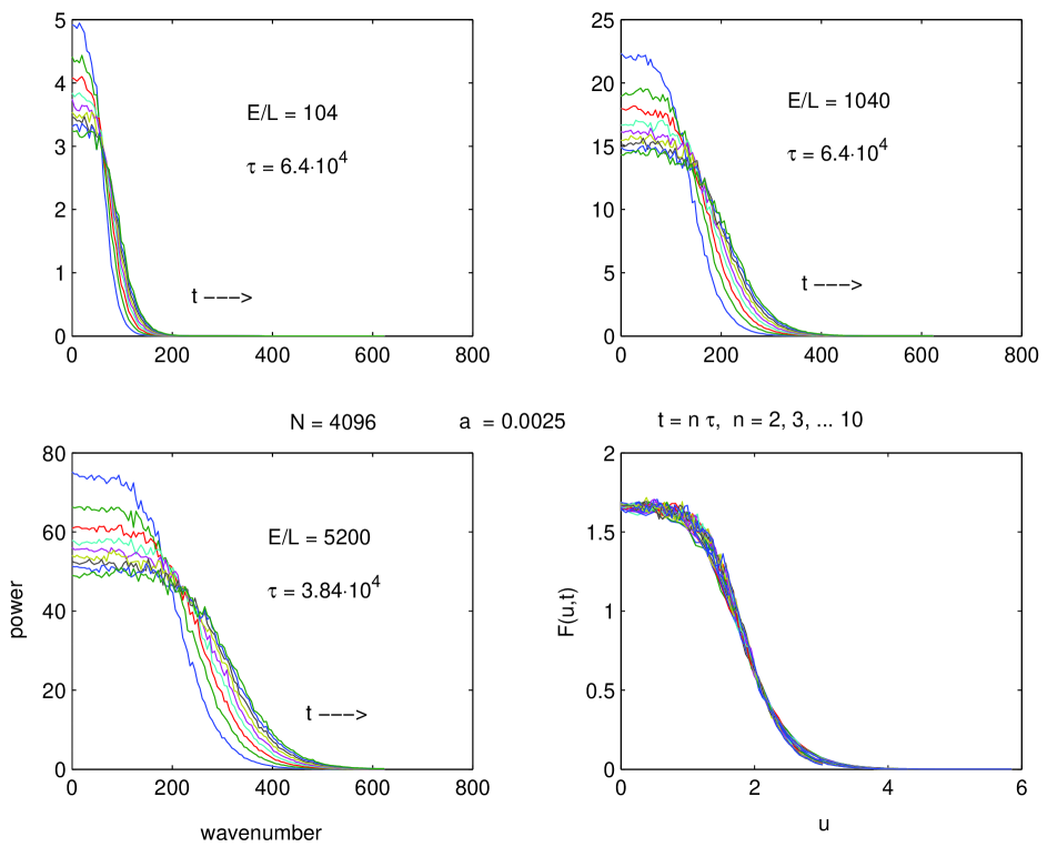
Figure 17: The ultraviolet cascade for $k\geq 0$ and three different values of the energy density (top and bottom-left). In all three cases and for all different times, a very good data collapse is obtained, upon rescaling, on the universal scaling function $F(u,0)$ (bottom–right).

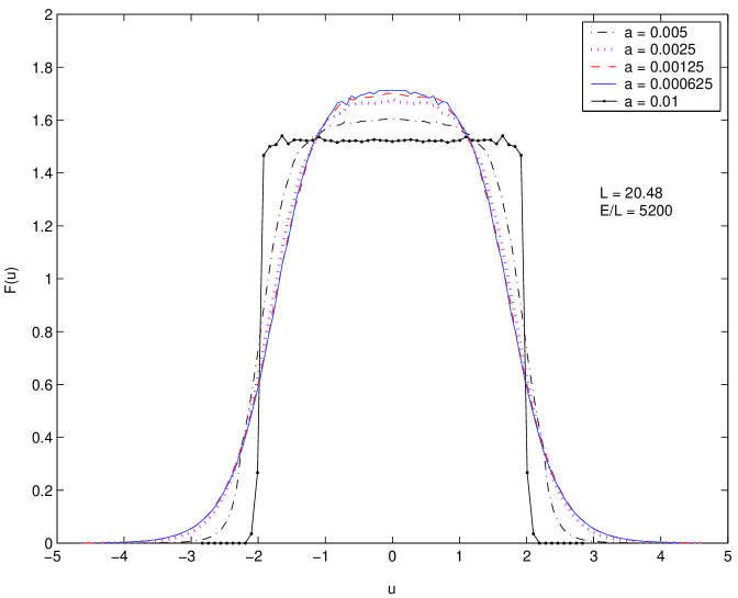
Figure 18: Numerical results for the universal function $F(u,v)$ obtained through time averages of $P(k,t)$ from $t=51200$ to $t=384000$, for several values of the UV cutoff, at fixed energy density. When $a=0.01$ the cascade is almost over and we obtain a profile very close to $F(u,1)$ [see eq.(110)]. When $a=0.005$ the bulk of the cascade reaches the UV cutoff, causing significant deformations. In the other cases the bulk of the cascade is still far away from the cutoff and $F(u,0)$ is approached. $F(u,0)$ is obtained in the continuum limit $a\to 0$.

Our exhaustive numerical analysis leads us to conclude the following picture for the cascade and the process of thermalization. For a wide range of initial conditions, lattice cutoff and energy density, there exists a scaling window for the cascade, namely a time interval $t_{1}\gg t\gg t_{0}$ characterized by the following properties:

• For $t_{1}\gg t\gg t_{0}$ so that $2\;\overline{k}(t)\ll\Lambda$ we find that $\overline{k}(t)$ is described by power–like behaviour in time, as shown for instance in fig.16, namely

  $$\overline{k}(t)\simeq h_{1}\;t^{\alpha}\;;$$ (103)

  where $\alpha$ is slowly growing with $E/L$, typically $0.21\leq\alpha\leq 0.25$ for $E/L\gtrsim 10$ , while $h_{1}\sim(E/L)^{\gamma}$, with $\gamma\sim 0.25$, for $E/L\gtrsim 10$. The numerical evidence suggests that both $\alpha$ and $\gamma$ depend on the initial conditions only through $E/L$.

• During the interval $t_{1}\gg t\gg t_{0}$ the front of the cascade is far away from the cutoff, namely $v\ll 1$ and $F(u,v)$ depends very weakly on $v$ therefore $F(u,2\,\frac{\overline{k}(t)}{\Lambda})$ is almost time independent. Hence, during this interval we can make the approximation $F(u,v)\simeq F(u,0)$ so that $P(k,t)$ satisfies the following scaling law with great accuracy [see fig. 17]

  $$P(k,t)\simeq\frac{1}{\overline{k}(t)}\,F\Big{(}\frac{k}{\overline{k}(t)}\,,0\Big{)}\quad\mbox{for}\quad a\;\overline{k}(t)\ll 1\;.$$ (104)

  Hence $P(k,t)$ satisfies a renormalization group-like relation for its time dependence, namely

  $$P(k,t)\simeq\frac{\overline{k}(t^{\prime})}{\overline{k}(t)}\;P\Big{(}\frac{\overline{k}(t^{\prime})}{\overline{k}(t)}\;k,\,t^{\prime}\Big{)}\;.$$ (105)

  and $F(u,0)$ plays the role of scaling function.

The behavior of $\overline{k}(t)$ as a function of the logarithm of time for several values of the lattice cutoff $a$ displayed in fig.16 shows a power-law behavior given by eq.(103) in the window $t_{1}\gg t\gg t_{0}$ and a saturation for times larger than $t_{1}$ (which depends on the lattice cutoff).

Proposing that, for very small lattice spacings and late times, $a\;\overline{k}(t)$ is solely a function of the combination $a\,t^{\alpha}$, namely

$$\begin{split}a\,\overline{k}(t)&=h(s)\;,\;s=a\;t^{\alpha}\;,\;a\to 0\;,\;t\to\infty\;,\\ h(s)&\simeq h_{1}\,s\;,\quad s\to 0\;;\end{split}$$ (106)

we find numerically the function $h(s)$ displayed in fig. 19 for $E/L=5200$ and in fig. 20 for $E/L=520$ and $E/L=104$. These results show quite clearly that $\alpha$ does depend, although quite weakly, on $E/L$. Actually, as explained in the Appendix, this scaling–based approach is more effective in the determination of $\alpha$ than direct fitting. Moreover, these results show that $h(s)$ is not universal, but depends on the initial conditions at least (and most likely only) through $E/L$.

In fact, it turns out that the data for $h(s)$ all collapse very well on a unique profile upon rescaling $s\to(E/L)^{\gamma}\,s$, if $\gamma=0.25$. In other words, for the average wavenumber the following double scaling form holds true when $E/L$ is large enough

$$\overline{k}(t;\,a;\,E/L)\simeq a^{-1}\,{\tilde{h}}\Big{(}a\,t^{\alpha}\,\left(\frac{E}{L}\right)^{\gamma}\Big{)}\;,$$ (107)

where ${\tilde{h}(s)}$ is now a universal function of order 1 with ${\tilde{h}(s)}\sim{\tilde{h}}_{1}s$ as $s\to 0$ and ${\tilde{h}}_{1}\sim 1.1$ [our numerical reconstruction of ${\tilde{h}}(s)$ is reported in fig. 21]. Therefore, a fairly good approximation for $\overline{k}(t)$ during the universal cascade ($t_{1}\gg t\gg t_{0}$) is given by,

$$\overline{k}(t)\simeq 1.1\;\left(\frac{E}{L}\right)^{\frac{1}{4}}\;t^{\alpha}\;.$$ (108)

with $0.21<\alpha<0.25$ according to the value of $E/L$ [see Table I].

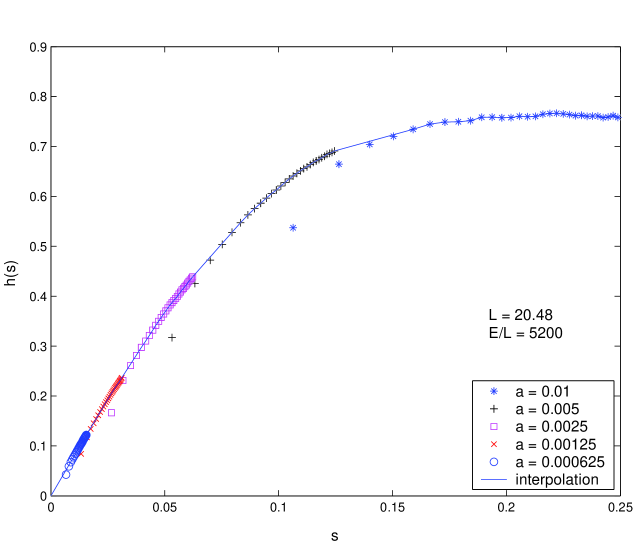
Figure 19: Numerical estimate of the function $h(s)$ obtained by interpolating the data of $a\;\overline{k}(t)$ vs. $s=a\;t^{1/4}$. Deviations occur here when the time $t$ is not large enough compared to the averaging interval and are not included in the interpolation.

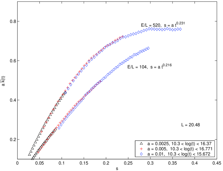
Figure 20: Data collapse over the scaling function $h(s)$ of $a\overline{k}(t)$ for $E/L=520$ and $E/L=104$.

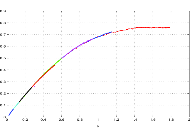
Figure 21: The double scaling function ${\tilde{h}}(s)$ reconstructed from several set of data at different $E/L$ and $a$.

The function ${\tilde{h}(s)}$ saturates for infinite time to the value $\pi/4$ which translates into the maximum value for the front wavevector $\overline{k}_{max}=\pi/4a=\Lambda/2$. Actually ${\tilde{h}}(s)$ in practice saturates already when $\gtrsim\pi/2$ (see fig. 21). Therefore we extract the thermalization time scale

$$t_{1}\simeq\Lambda^{1/\alpha}\,(E/L)^{-\gamma/\alpha}\;,$$ (109)

at which $2\,\overline{k}(t_{1})\lesssim\Lambda$. For $t\gg t_{1}$ the power spectrum $|\tilde{\pi}_{k}|^{2}$ features a plateau for all wavevectors up to the cutoff, thus describing the thermal equilibrium state.

As far as the shape function $F(u,v)$ is concerned, we see from fig. 18 that for $v\ll 1$ it features a bell-shaped profile with exponentially small tails for large $u$,

$$F(u,v)\simeq{\cal C}\;\exp[-\gamma(v)|u|]\;,\quad|u|\gg 1\;,$$

with $\gamma(0)\sim 2$ and ${\cal C}$ a constant. As $v$ increases, the tails decrease even faster, the lateral walls steepen and the central region flattens. Finally, as $v\to 1$, which corresponds to complete thermalization, we have [see eqs.(101) and (IV.1)]

$$\lim_{t\to\infty}P(k,t)=2a\;,\quad F(u,1)=\begin{cases}\pi/2&|u|<2\\ 0&|u|>2\end{cases}\;,$$ (110)

to be compared to the approximation $F(u,v)\simeq F(u,0)$ valid in the scaling window. Strictly speaking, the function $F(u,0)$ is truly universal in the continuous limit where $v=\frac{4}{\pi}\;\overline{k}(t)\;a\to 0$. However, one can see a very good approximation to $F(u,0)$ in fig. 18 for the plot at the smallest $a=0.000625$.

Finally, by construction, $F(u,v)$ is even in $u$ and must satisfy, following eqs.(97) and (98),

$$\int_{0}^{2/v}du\,F(u,v)=\int_{0}^{2/v}du\,u\,F(u,v)=\pi\;,$$

for any value of $v$.

Summarizing, after the transient stage, the effects of the initial conditions on $P(k,t)$ are entirely accounted for by the average wavenumber $\overline{k}(t)$, which fixes the scale of the universal ultraviolet cascade with shape described by $F(u,v)$. For $v\ll 1$, namely when the front of the cascade is far away from the cutoff, the function $F(u,0)$ is universal as shown explicitly by the collapse of the data for several values of the initial energy density onto one function in fig. 17.

IV.2 Time dependent effective temperature and local equilibrium

The shape and universality of the power spectrum $\overline{|\tilde{\pi}_{k}|^{2}(t)}$ featuring a flat plateau behind the wake of the cascade leads to the definition of the effective temperature $T_{\rm eff}(t)$ as the height of the plateau. The interpretation of this temperature is that for $t\gg t_{0}$ but well before the true thermalization time $t_{1}$, there is an description in terms of local equilibrium (local in Fourier space) at the effective temperature $T_{\rm eff}(t)$.

In order to firmly state this conclusion, however, we must understand if the other criteria for thermalization established in section II.10 are fulfilled.

Combining eqs.(96) and (102) we can write the $\pi$ power spectrum as

$$\overline{|{\tilde{\pi}}|^{2}}(k,t)=\frac{\overline{\pi^{2}(t)}}{\overline{k}(t)}\;F\Big{(}\frac{k}{\overline{k}(t)},\,\frac{2\;\overline{k}(t)}{\Lambda}\Big{)}\;.$$

For $t_{0}\ll t\ll t_{1}$, within the scaling window, this is well approximated using eq.(103) as

$$\overline{|{\tilde{\pi}}|^{2}}(k,t)\simeq\frac{\overline{\pi^{2}(t)}}{h_{1}\;t^{\alpha}}\;F\Big{(}\frac{k}{h_{1}\;t^{\alpha}},\,0\Big{)}\;.$$

Now, for any fixed $k$ in the bulk of the cascade and large enough $t$ (but still $t\ll t_{1}$), taking into account the flat profile of $F(u,0)$ around $u=0$, we can write

$$\overline{|{\tilde{\pi}}|^{2}}(k,t)\simeq\frac{\overline{\pi^{2}(t)}}{h_{1}\;t^{\alpha}}\,F(0,\,0)\equiv T_{\rm eff}(t)\;,$$

which is indeed $k-$independent. Moreover, the observed change in time of the integrated power spectrum ${\overline{\pi^{2}}(t)}$ is not as important [see figs. 2 and 4]. It slowly decreases to its asymptotic value which agrees with the thermal equilibrium value $T/(2a)$ [see eq.(99)]. Hence, to leading order in $t$ (but always with $t\ll t_{1}$) we may write:

$$T_{\rm eff}(t)\simeq\frac{E}{L}\;\frac{F(0,0)}{h_{1}\,t^{\alpha}}\;.$$ (111)

Finally, using the large $E/L$ behavior of $h_{1}$ [see eq.(107)], we arrive at

$$T_{\rm eff}(t)\simeq T_{1}\,\Big{(}\frac{E}{L}\Big{)}^{1-\gamma}t^{-\alpha}\;,$$ (112)

The constant $T_{1}=F(0,0)/{\tilde{h}}_{1}$ is estimated to be $T_{1}\simeq 1.55$, very close to $\pi/2$. We recall also that $\alpha$ is weakly dependent on $E/L$ for $E/L\gtrsim 10$, saturating approximately at $0.25$ for large $E/L$, and that $1-\gamma\simeq 3/4$ quite precisely from the scaling argument of eq.(107). Therefore, fairly good approximations for $t_{1}$ and $T_{\rm eff}(t)$ are given by,

$$t_{1}\simeq\frac{L\,\Lambda^{4}}{E}\;,\quad T_{\rm eff}(t)\simeq\frac{\pi}{2}\left(\frac{E}{L}\right)^{3/4}\;t^{-\alpha}\;.$$ (113)

The identification of the effective temperature allows us to study whether the other observables, such as $\overline{\phi^{2}(t)}$, $\overline{\phi^{4}(t)}$ or the correlation function $\overline{\phi\phi}(x,t)$, depend on this effective temperature in a manner consistent with local equilibrium. A numerical analysis reveals that indeed to high accuracy we have [see figs. 22 and 23]

$$\overline{\phi^{2}}(t)=\langle\phi^{2}\rangle(T_{\rm eff}(t))\;,\quad\overline{\phi^{4}}(t)=\langle\phi^{4}\rangle(T_{\rm eff}(t))\;,$$ (114)

in terms of the equilibrium functions $\langle\phi^{2}\rangle(T)$ and $\langle\phi^{4}\rangle(T)$ plotted in fig. 1 early times (but $t\gg t_{0}$), that is high effective temperature these reproduce the thermal equilibrium results given by eq.(77), while for late times and large UV cutoffs, that is low effective temperature, these agree with the free field results (60)-(63).

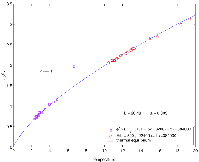
Figure 22: Effective thermalization of $\overline{\phi^{2}}(t)$.

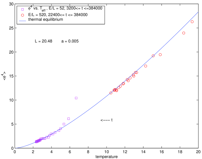
Figure 23: Effective thermalization of $\overline{\phi^{4}}(t)$.

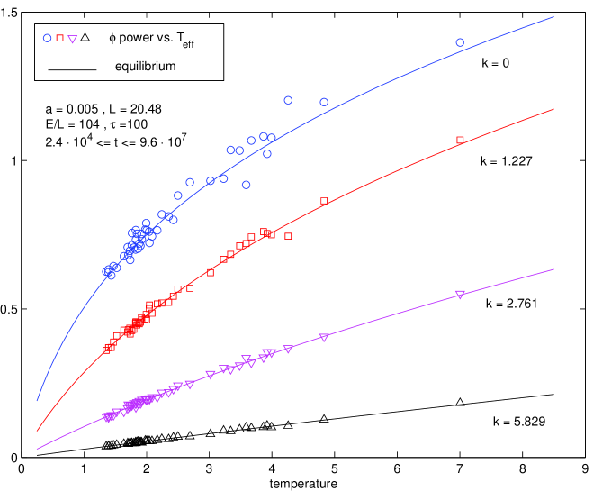
Figure 24: Effective thermalization of $\overline{|{\tilde{\phi}}|^{2}}(k,t)$ for different values of $k\ll 2\,\overline{k}(t)$ .

A more precise analysis can be performed on $\overline{\phi\phi}(x,t)$, or better on its Fourier transform $\overline{|{\tilde{\phi}}|^{2}}(k,t)$. Indeed, as evident from fig. 24, we find that for $k\ll 2\,\overline{k}(t)\ll\Lambda$ and $t\gtrsim t_{0}$

$$\overline{|{\tilde{\phi}}|^{2}}(k,t)\simeq{\tilde{G}}(k,T_{\rm eff}(t))\;,$$ (115)

in terms of the equilibrium distribution ${\tilde{G}}(k,T)$. For $k$ too close to the front of the cascade $k<2\,\overline{k}(t)$ effective thermalization has not occurred yet, but this does not affect significantly quantities like $\overline{\phi^{2}(t)}$ in which all wavenumbers are summed over, since the equilibrium ${\tilde{G}}(k,T)$ vanishes as $T/k^{2}$ for large $k$. It instead affects significantly quantities like $\overline{\phi^{\prime 2}(t)}$, since the $\phi$ equilibrium power spectrum $k^{2}\;{\tilde{G}}(k,T)$ goes to $T$ for large $k$.

The physical meaning and interpretation of the effective temperature and the description in terms of local equilibrium at this temperature behind the front of the ultraviolet cascade applies solely to long wavelength physics. Namely the wavevectors behind the front of the cascade $k<2\;\overline{k}(t)$ can be considered to be thermalized by the mode mixing entailed by the interaction. Physical observables that do not depend on the cutoff are described in terms of this local thermal equilibrium concept.

This description in terms of a universal cascade in local thermal equilibrium at an effective temperature $T_{\rm eff}(t)$ applies for $t\gg t_{0}$ up to the time $t_{1}$ at which the front of the cascade $2\;\overline{k}(t)$ reaches the cutoff. From this time onwards (during the fourth stage, see sec. III.4) the power spectrum $\langle|\tilde{\pi}_{k}|^{2}\rangle$ is no longer universal and is sensitive to the cutoff.

There is a clear separation between the time scale $t_{0}\sim 50000$ where the cascade forms with the effective time-dependent temperature $T_{\rm eff}(t)$ and the much longer time scale $t_{1}\propto a^{-4}$ which signals that the front of the cascade is near the cutoff and the end of the universal cascade.

Thermalization does continue beyond $t_{1}$ during the fourth stage [see sec. III.4] and the power spectrum $\langle|\tilde{\pi}_{k}|^{2}\rangle$ eventually becomes $T\;\Theta(\Lambda-k)$ with $T$ the true equilibrium value of the temperature (determined by the energy density) at infinite time. Thus true thermalization takes an infinitely long time.

Hence the dynamics for long-wavelength phenomena can be described to be in local thermodynamic equilibrium for $t>t_{0}$ at a time dependent temperature $T_{\rm eff}(t)$ while short wavelength phenomena on the scale of the cutoff will reach thermalization only at a much later time scale $t\gg t_{1}$.

The ratio $\frac{\langle\phi^{2}\rangle^{2}}{\langle\phi^{4}\rangle}$ plotted in thermal equilibrium as a function of $T$ in fig. 1 provides a simple test of effective thermalization. This ratio increases monotonically from its zero temperature value $\frac{1}{3}$ up to its infinite temperature limit $0.37077\ldots$ [eq.(70)]. Therefore, a necessary condition for effective thermalization is that

$$\frac{1}{3}\leq\frac{[\overline{\phi^{2}}(t)]^{2}}{\overline{\phi^{4}}(t)}\leq 0.37077\ldots$$ (116)

We depict in fig.25 the ratio $\frac{\langle\phi^{2}\rangle^{2}}{\langle\phi^{4}\rangle}(t)$ as a function of the logarithm of the time $t$ for three values of $E/L$. Effective thermalization may start only when the ratio falls within the inequality (116). We see from fig. 25 that for $E/L\gtrsim 10$ this happens around $\ln t\sim 9$ which is about the begining of the universal cascade [see sec. III.4]. For $E/L=3.669$ effective thermalization starts much later around $\ln t\sim 12$. More generally, we find for $E/L\lesssim 10$ that thermalization is significantly delayed.

Figure 25: The ratio $\frac{\langle\phi^{2}\rangle^{2}}{\langle\phi^{4}\rangle}(t)$ as a function of the logarithm of the time $t$ for $E/L=3424,\;50.28$ and $3.669$ for $L=20$ and $a=0.01$. This ratio in thermal equilibrium takes values between the low temperature limit $1/3$ and the high temperature limit $0.37077\ldots$ depicted as a dotted line. Hence, effective thermalization may start only when the ratio falls within such strip [see eq.(116)]. For $E/L=3.669$ effective thermalization only starts for $\ln t>20$.

V Conclusions and discussions

In this article we have studied the approach to equilibrium in the classical $\phi^{4}$ theory in $1+1$ dimensions with the goal to understand the physical process that lead to thermalization and to establish criteria for the identification of a thermalized state in a strongly interacting theory. After discussing the classical theory as the limit of the quantum field theory, we exploited the equivalence of the classical partition function to the transfer matrix for the quantum anharmonic oscillator. A body of established results on the spectrum of the quantum anharmonic oscillator allows us to obtain exact results for low, high and intermediate temperatures which furnish a yardstick and a set of criteria to recognize thermalization from the physical observables. We compared these exact results to those obtained for the same quantities in the Hartree approximation and found that this simple approximation describes the equilibrium properties of the theory remarkably accurately, to within $10\%$ for most observables. We point out that in the high temperature, or equivalently the large energy density regime there is a strong renormalization of the single particle frequencies.

After studying the equilibrium properties, we presented a method to solve the equations of motion based on the dynamics on a light–cone lattice. This method is particularly suitable to study the evolution in field theories within the setting of heavy ion collisions where the initial dynamics is mainly along the light cone, it is very stable and conserves energy to high accuracy. The equations of motion for the classical field where solved with a broad range of initial conditions and energy densities, corresponding to microcanonical evolution. In all of these initial conditions the initial energy density was stored in few (or a narrow band) of long wavelength modes.

Our main results reveal several distinct stages of evolution with different dynamical features: a first transient stage during which there are strong fluctuations is dominated by the interaction term, mode mixing begins to transfer energy from small to larger wavevectors. A second stage is distinguished by the onset of a very effective transfer of energy to larger wavevectors, this is an energy cascade towards the ultraviolet. During this second stage the interaction term $\phi^{4}$ diminishes and eventually becomes smaller than the spatio-temporal gradient terms. At the end of this stage $\phi^{4}\ll\phi^{\prime 2};\pi^{2}$. The third stage is dominated by the ultraviolet cascade and the power spectrum of the canonical momentum $|\tilde{\pi}_{k}|^{2}$ features a universal scaling form. The cascade is characterized by a front $\overline{k}(t)$ which slowly moves towards the ultraviolet cutoff as $\overline{k}(t)\simeq(E/L)^{\frac{1}{4}}\;t^{\alpha}$ with $\alpha\sim 0.25$ an almost universal exponent independent of the lattice spacing and the details of initial conditions but weakly dependent on the energy density. During this stage and while the front of the cascade is far away from the cutoff, the power spectrum is universal. Behind the front of the cascade the power spectrum is that of thermal equilibrium with an effective temperature $T_{\rm eff}(t)$ which slowly decreases towards the equilibrium value. During this stage we find that all observables have the same functional form as in thermal equilibrium but with the time dependent effective temperature. Namely the wake behind the front of the ultraviolet cascade is a state of local thermodynamic equilibrium. This stage of universal cascade ends when the front is near the cutoff, at a time scale $t_{1}\simeq\frac{L}{E}\;a^{-\frac{1}{\alpha}}$ with $a$ the lattice spacing.

The dynamics continues for $t>t_{1}$ but is no longer universal, true thermalization is actually achieved in the infinite time limit and occurs much slower than in any previous stage.

Thus we find that thermalization is a result of an energy cascade with several distinct dynamical stages. Universality and scaling of power spectra emerges in one of the later stages and local thermodynamic equilibrium is associated with this stage. While we find scaling and anomalous dynamical exponents we did not find any turbulent cascade.

We concur with previous studies that thermalization is indeed achieved but on extremely long time scales, however our study reveals that virialization starts to set earlier than local thermodynamic equilibrium.

It is important to emphasize that the universal cascade described above is different from a turbulent regime described in ref.tkachev where the classical massless $\phi^{4}$ model was studied in $3+1$ dimensions. In that reference, the spectrum for the distribution of particles defined with respect to the Hartree frequencies is studied and the numerical results are interpreted in terms of wave turbulence and fit to a Kolmogorov spectrum in tkachev .

We do not find a turbulent spectrum in the power spectra of the field or its canonical momentum, instead we find local thermodynamic equilibrium with an effective time dependent temperature which diminishes slowly. While our study in $1+1$ dimensions reveals local thermal equilibrium in contrast to the results of ref.tkachev in the $3+1$ dimensional case, there are several features in common: a)extremely long thermalization time scales, as compared to the two natural time scales $m^{-1}$ or $T^{-1}$, b) a cascade of energy towards the ultraviolet and a cascade front that evolves towards the cutoff as a function of time. This latter feature can be gleaned in fig. (2) in ref.tkachev .

The theory of weak wave turbulence which describes the dynamical evolution in terms of kinetic equations leads to a turbulent spectrum for nonrelativistic and nonlinear wave equations as the three wave equationlvov . It was argued in ref.son that the non-equilibrium evolution in $\phi^{4}$ in $3+1$ dimensions but in the small amplitude regime features a scaling behavior and a power law albeit different from the one with $\alpha\sim 0.21-0.25$ that we find in $1+1$ dimensions.

More recentlynewell , a study of local wave turbulence for a system dominated by four-wave interactions, again via wave kinetic equations and following the methods of ref.lvov , reports the formation of cascades that feature a front that moves forward in time, the wake behind the front features a Kolmogorov-Zakharov spectrum of weak turbulence. The behavior of a moving front found in ref.newell is similar to the front of the cascade that we find numerically, but the wake is different, we find local thermodynamic equilibrium, while in ref.newell the distribution is of the Kolmogorov type.

While a kinetic description may not reliable during the first stage of the dynamics, a suitable kinetic description in terms of a distribution function for particles of the (strongly) renormalized frequency may be available during the second and third stages. We comment on these and other issues below.

Discussions and comments:

As discussed in section II, the classical limit must be understood with a lattice (or ultraviolet) cutoff to avoid the Rayleigh-Jeans divergence. For a finite energy density the naive continuum limit leads to a vanishing temperature in equilibrium. Furthermore the classical approximation is valid when occupation numbers are large. In the cases under study for large energy density and initial conditions for which the energy is stored in long-wavelength modes, the classical approximation is valid and reliable for small wavevectors. Our study reveals that the cascade of energy proceeds very slowly after the first stage, thus suggesting that the dynamics after the first stage could be studied within a kinetic approach. However, such kinetic approach should include the strong renormalization of the single particle frequencies in order to define the slowly varying distribution functions.

Another result of our study is that the simple Hartree approximation is in remarkably good agreement with the exact results in equilibrium.

Thus we conjecture that the following scenario for studying thermalization in a quantum field theory may prove suitable to understanding the dynamics from initial conditions that entail large occupations for long-wavevectors: study the numerical evolution in the quantum Hartree approximation up to the time scale at which the interaction and consequently the evolution becomes on long time scales. At that stage read out the occupation numbers for suitably defined single quasiparticles. Obtain the kinetic equations for the evolution of these quasiparticle occupations for a weakly coupled theory, and continue the evolution via these kinetic equations towards final equilibration using the occupation numbers at the end of the Hartree evolution.

This program, if proven suitable, is certainly much more economical and efficient than trying to implement more sophisticated and calculational intensive approximation schemes that lead to non-local update equations. This suggestion is analogous to that advocated inson2 for the evolution after nucleus-nucleus collisions.

We highlight that we do not find a thermalization threshold as found in the study of FPU chainsFPU ; varios . Namely, even for low values of the energy density the $\phi^{4}$ theory reaches thermal equilibrium for very long times. Indeed, the thermalization scale $t_{1}$ diverges in the $a\to 0$ limit [see eq.(113)]. The fact that the thermalization slows down when $\overline{k}(t)$ approaches the UV cutoff (Brillouin zone) can be understood as follows. The UV cascade can be understood as follows. The equation of motion (5) for the Fourier component of the classical field with wavevector $k$ features the non-linearity $\sum_{k_{1}}\sum_{k_{2}}\tilde{\phi}_{k_{1}}\;\tilde{\phi}_{k_{2}}\;\tilde{\phi}_{k-k_{1}-k_{2}}$. Thus, if initially the amplitude corresponding to a wavevector large $k$ is small, the modes with small $k$ and large amplitude lead to a large non-linearity that acts as a source for the amplitude with $k$. In this manner, if the initial power spectrum is localized at small wavevectors the amplitude of the higher modes increases via the non-linearities and the transfer of energy by mode mixing. By periodicity the sum $k-k_{1}-k_{2}$ is constrained to be in the first Brillouin zone. Therefore when $k-k_{1}-k_{2}$ is larger than the cutoff, periodicity implies that this sum must be folded back inside the first Brillouin zone by adding a vector in the reciprocal lattice, namely $\pi/2a$. Hence once the amplitudes for wavevectors near the cutoff are beginning to be large, the non-linearity transfer the energy to low momentum modes.

Hence, the cascade mechanism is less efficient for $k\lesssim\Lambda$ than for $k\ll\Lambda$.

While we have focused on the study of the dynamics in a classical field theory with a cutoff as a timely and interesting problem all by itself, the applicability of our results to the realm of quantum field theory descriptions of early Universe cosmology and ultrarelativistic heavy ion collisions must be discussed.

Classical field theory is likely to describe the QFT non-equilibrium dynamics at least in the cases in which the occupation numbers are very large. Strongly out of equilibrium when a temperature cannot yet be defined, the classical description is valid for the range of momenta corresponding to large occupation numbers. Near equilibrium this would be the case for frequencies much smaller than the temperature. Our study reveals that effective thermalization is reached for times $t>t_{0}$ with a time dependent effective temperature. Hence, our classical results should apply to QFT for modes with frequencies much smaller than the effective temperature.

In order to extract a criterion for the validity of the classical approximation we must revert to the physical variables $T_{p},\;a_{p}$ related to the rescaled variables used in this study as in eqs. (2)-(8), namely $T_{p}=m^{3}\;T/\lambda,\;a_{p}=a/m,\;k_{p}=m\;k$. $T_{p}$ is the temperature in physical units and the physical momenta in the lattice are restricted to be $-\pi/a_{p}\leq k_{p}\leq\pi/a_{p}$ (first Brillouin zone).

The exact equilibrium results obtained above indicate that the exact equilibrium frequencies are of the form $\omega(k)=\sqrt{k^{2}+b\,T^{2/3}}$ with $b$ of order 1, where $T$ is the dimensionless rescaled temperature $T=\lambda\;T_{p}/m^{3}$. While in the classical theory the mass and coupling constant can be absorbed in an overall rescaling of the dimensionful parameters and the amplitude of the fields, that is not the case in the quantum theory where the amplitude of the fields and their canonical momenta are fixed by the commutation relations. Thus a comparison of the classical and quantum theory requires reverting to the physical variables. Moreover, the dimensionless ratio $\lambda/m^{2}$ plays a rôle in the discussion as we show below.

By following the numerical evolution of single modes it is easy to see that for all modes in the bulk of the cascade, where local equilibrium holds, the time-dependent dimensionless frequencies have the expected form

$$\omega_{k}(t)=\sqrt{k^{2}+b\;T_{\rm eff}(t)^{2/3}}$$

We emphasize that the cascade corresponds to a state of local equilibrium with the effective temperature $T_{eff}(t)$ which is much larger than the final thermodynamic equilibrium temperature.

A simple criterion for the validity of the classical approximation in QFT is that

$$T_{\rm p,eff}(t)\gg\omega_{p}(\overline{k}_{p}(t))$$ (117)

where $\omega_{p}(k_{p})=\sqrt{k_{p}^{2}+b\,[\lambda\;T_{\rm p,eff}(t)]^{2/3}}$ are the dimensionful frequencies. In dimensionless variables eq.(117) takes the form,

$$\frac{m^{3}}{\lambda}T_{\rm eff}(t)\gg m\,\sqrt{\overline{k}(t)^{2}+b\;T_{\rm eff}(t)^{2/3}}$$ (118)

It is enough to discuss the modes at the wake to see the applicability of the classical approximation since $k<\overline{k}(t)$ for the modes in the cascade. At times early enough, in regimes such that the plateau is already formed but $\overline{k}(t)\ll T_{\rm eff}(t)^{1/3}$, eq.(117) holds provided $T_{\rm eff}(t)\gg(\lambda/m^{2})^{3/2}$, which is certainly true for $\lambda$ small enough.

On the other hand if $\overline{k}(t)\gg T_{\rm eff}(t)^{1/3}$ the classical approximation will be valid provided

$$\frac{m^{2}}{\lambda}\;T_{\rm eff}(t)\gg\overline{k}(t)$$ (119)

Using our late time estimates eqs. (108), (113) for $\alpha=0.25$ one obtains the condition

$$t\ll t_{Q}\;,\quad t_{Q}\sim\frac{m^{4}\,E}{\lambda^{2}\;L}=\frac{E_{p}}{\lambda\,L_{p}}$$ (120)

This shows that for sufficiently small coupling constant and fixed UV cutoff $\Lambda=\pi/a_{p}$ the classical approximation could be valid up to full thermalization, that is $t_{Q}\gg t_{1}$, which using the first of eq. (113) is equivalent to the condition

$$\frac{E}{L}\gg\frac{\lambda}{m^{2}\;a^{2}}$$

Recalling that $E/L\simeq T/(2a)$, this is nothing but $T_{p}\,a_{p}\gg 1$. In fact, as the front of the cascade moves towards the cutoff, for a fixed cutoff, the classical approximation will continue to be valid for all modes behind the wake of the cascade if $T_{p}\;a_{p}\gg 1$.

The validity of the classical approximation for $T_{p}\,a_{p}\gg 1$ is well known in the elementary theory of harmonic solids where phonons are the elementary excitations. In the Debye model of solids the classical limit is valid for $T_{p}>T_{D}$ where $T_{D}\propto\pi/a_{p}$ is the Debye Temperature (and $\pi/a$ is the edge of the first Brillouin zone, namely the maximum momentum)solid .

As per the discussion in section II.9 the non-linearities are subdominant for $Ta^{3}\ll 1$, condition which all but guarantees the cascade [see discussion in section II.9]. Therefore, the validity of the classical approximation is warranted provided,

$$T_{p}\,a_{p}\gg 1\quad\mbox{or ~{}equivalently}\quad T\,a\gg\frac{\lambda}{m^{2}}\;,$$ (121)

which is the same condition for the validity of the classical limit in elastic solids.

Since our results are valid for $T\;a^{3}\ll 1$ the classical results obtained here apply in the quantum theory for a fixed cutoff in the whole dynamical range where eq.(119) is valid.

We have studied the dynamical evolution in a broad range of parameters from $0.001\leq Ta\lesssim 1$ (with $Ta^{3}\ll 1$) and found a similar behavior for the dynamics during the stage of the universal cascade. Therefore, our classical results applies in QFT provided one chooses values of $\lambda/m^{2}$ fulfilling eq.(121) for the values of $Ta$ indicated in the respective plots. Indeed, our classical results turn to be relevant for the weakly coupled quantum field theory. Otherwise, quantum effects certainly appear in the process of thermalizationberges ; serreau . Nonetheless, even in the continuum limit at fixed coupling constant, when inevitably $T_{p}\,a_{p}\to 0$, it is conceivable that, as long as $t\ll t_{Q}$, the classical approximation is quite accurate for all modes in the bulk of the cascade. One should expect that the shape of the cascade at the forefront indeed depends sensibly on quantum effects, since occupation numbers fall off rapidly across it. But the rate at which the plateau behind decreases is most likely almost purely classical, at least until occupation numbers are high, that is for $t\ll t_{Q}$, when the effective temperature is high enough.

Hence, in the quantum field theory with initial conditions strongly out of equilibrium with a power spectrum featuring large occupations for long wavelengths we expect that the initial stages of the dynamics will likely be well described by the classical field theory. In this case we expect a cascade to form, the modes behind the front will be well described by the classical field theory, whereas in the theory with a large cutoff, the modes with small occupation in front of the cascade all the way to the cutoff will require a quantum description. The backreaction of these quantum modes onto the long-wavelength modes will modify the time evolution of the cascade.

In the quantum $\phi^{4}$ theory we expect that the time scale for complete thermalization to be finite even in the continuum limit. While in the classical limit the equilibrium power spectrum for the field falls off with a power law and that of the canonical momentum is flat, hence sensitive to the cutoff, in the quantum theory the exponential suppression will make the theory insensitive to the cutoff in the limit $T\;a\ll 1$. Hence, we conjecture that time scale for complete thermalization diverges in the continuum quantum theory when $\hbar\to 0$. Furthermore, we expect faster thermalization in the quantum theory since zero point fluctuations imply finite amplitude for all modes in the initial state.

The numerical studies previously reported on the dynamics of classical and quantum field theories patkos -marcelo have not yet focused on studying the mechanism of energy transfer from long to short wavelengths as a function of time, although ref.marcelo reported the emergence of spatio-temporal structures. It would indeed be interesting to study if the universal cascade found in the classical theory remains at least during some early and intermediate stages in the quantum theory.

Our study in conjunction with a previous body of work clearly suggests that thermalization, at least in this scalar theory, occurs on extremely long time scales, much longer than the natural scales $m^{-1}\,,\,T^{-1}$. However, local thermodynamic equilibrium with a slowly decreasing effective temperature $T_{\rm eff}(t)$ emerges relatively soon. This result all by itself raises important questions on the current assumptions on thermalization both in cosmology as well as in heavy ion collisions. If thermalization involves a time dependent effective temperature, both in cosmology as well as in the formation and evolution of the quark gluon plasma, there are immediate phenomenological consequences and a reassessment of the current assumptions and models is called for.

An intense program to study these issues and their impact on both fields is therefore warranted.

VI Appendix

We provide here more details on our numerical calculations. They were performed on a cluster of personal computers at LPTHE-Paris and at the Physics Department of Milano–Bicocca. The computers were used in parallel with different values of relevant parameters on each one of them.

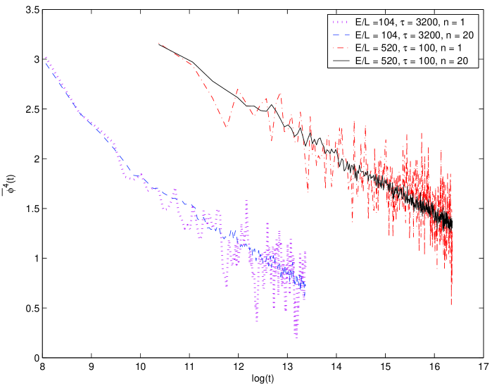
Figure 26: Comparison of different averagin methods. $n$ is the number of initial conditions in each average.

In our numerical evolution the number of iterations of the discrete system, eq.(85), is $t_{\rm max}/(2\,a)$ when evolving from $t=0$ up to $t=t_{\rm max}$. The computer time increases for smaller spacing also because at fixed size $L$, smaller $a$ implies larger $N=L/(2a)$. This implies a number of operations of order $a^{-2}$. Moreover, if fast Fourier transforms are performed every iteration, to average the power spectra over the time intervals $[t,t+\tau]$ covering completely the time span from $t=0$ up to $t=t_{\rm max}$, then altogether the computer time scales as $a^{-2}\log\frac{1}{a}$ for small $a$. Actually, when also averages over initial conditions are performed, it turns out that $\tau$ need not be so large as to provide a complete covering, since the average over initial conditions is much more effective in reducing fluctuations than averaging in time [see fig 26]. In other words, it is sufficient to consider time intervals $[t,t+\tau]$ that cover only a relatively small part of the full time span from $t=0$ until $t=t_{\rm max}$. This implies that computer time really scales just as $a^{-2}$ for small $a$.

As pointed out in sec. III.5 we have two methods to compute $|{\tilde{\phi}}_{k}(t)|^{2}$. Either, to extract the field $\phi(x,t)$ from the lattice fields $F(n,s)$ and $G(n,s)$, Fourier–transform it to ${\tilde{\phi}}_{k}(t)$ and then perform all needed averages on $|{\tilde{\phi}}_{k}(t)|^{2}$. Or to directly compute the averages of the correlations of $F(n,s)$ and $G(n,s)$ and extract from them the correlations $\overline{\phi\phi}(x,t)$ and $\overline{\pi\pi}(x,t)$. Thanks to the exceptional scaling properties of the Fast Fourier Transform, the first method is actually preferable to the second, if the space average in eq.(95) is really performed and very extensive time averages are considered. However, as just explained, the time averages can be greatly reduced when averaging on numerous enough initial conditions.

We have seen in the previous sections that the mean wavenumber $\overline{k}(t)$ plays a central role in the description of the UV cascade. However, the numerical determination of the exponent $\alpha$ and of the amplitude $h_{1}$ for the time behaviour of $\overline{k}(t)$ in the scaling window, eq.(103) or, even more generally, in the determination of scaling function $h(s)$ in eq.(103) is a nontrivial matter. This is due to the characteristic fluctuations of the data that limit the control of the sistematic effects caused by the initial transient, by the scaling violations due to the UV cutoff and by the averaging over time intervals when the time is not much larger than interval length $\tau$. This type of fluctuations can be systematically reduced by enlarging the set of initial conditions over which we average, but are still present in a significant way for the number (typically 20 to 30) of initial configurations we used.

We identify the initial transient in $\overline{k}(t)$ by a self–consistent fitting procedure. Suppose a very good fit has been obtained for the data points at times larger than a certain time $\overline{t}$ (the actual fitting procedure is described below). Then we can see if and how much the data at $t<\overline{t}$ deviate from the fitting function. If the fit starts to worsen immediately before $\overline{t}$ and in a steady manner towards $t=0$, then the transient cannot be fully disentangled from the fitting errors and $\overline{t}$ needs to be increased until we find that the fit remains quite good for a while before $\overline{t}$ and then worsen in rather abrupt way. The time at which this worsening occurs provides an alternative estimate of the time scale $t_{0}$ introduced in sec. III.4 to signal the end of the transient and the start of the UV cascade that will become universal for $t\gg t_{0}$. Using the parametrization

$$\overline{k}(t)=h_{1}\,t^{\alpha}\,[1+g(t)]\;,$$

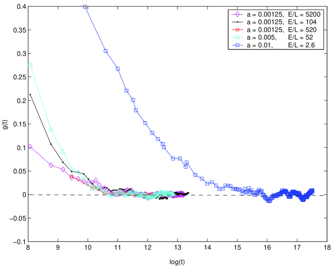
Figure 27: Numerical determinations of the function $g(t)$ that describes the initial transient for several values of $E/L$.

can then (approximatively) read $t_{0}$ out of the plot of $g(t)$ vs. $t$ [see fig 27]. We see that $\log t_{0}\lesssim 11$ (in agreement with what found in sec. III.4 for other observables) more or less independently on $E/L$ as long as $E/L\geq 52$. When $E/L=2.6$, $t_{0}$ is much larger instead, $\log t_{0}\sim 15$, as found also for the other observables. Notice that, when $E/L=2.6$, $\overline{k}(t)$ is very well fitted for $\overline{t}<t<t_{\rm max}$, with $\log\overline{t}\sim 14.5$ and by $\log t_{\rm max}\sim 17.5$ by the pure power law (103) of the scaling window, but with a power $\alpha\sim 0.186$ definitely smaller than those at higher energy densities.

Having disposed of the initial transient, we now turn to the fitting procedure to determine $h_{1}$ and $\alpha$. As a matter of fact, the simple, direct fitting of the numerical data of average wavenumber $\overline{k}(t)$ with eq.(103) is not quite precise, even when the scaling window is identified. For instance, the almost linear behaviour in the log–log scale for smaller values of the spacing $a$ is evident from fig. 16, but the actual values of $\alpha$ and of $h_{1}$ are poorly fixed in this simple fitting approach.

To give an idea of the situation, let us consider a specific example. In a parallel run of 20 evolutions from $t=0$ to $t=1.28\ldots\;10^{7}$, with $a=0.0025$ and $E/L=520$, each one starting from the same initial wavenumber $k_{i}$’s filled, but with randomly chosen amplitude and phases [according to the discussion in sec. III.2], a $20\times 400$ matrix $M$ of data for $\overline{k}(t)$ is obtained. Each row of $M$ corresponds to a given choice of initial conditions and the $n-$th column contains the values of the mean wavenumber at $t=n*\Delta t$ for $n=1,2,\ldots,400$ and $\Delta t=32000$. In this runs the time average intervals are rather small ($\tau=100$) compared to the data taking interval $\Delta t$ and so they cause a negligible sistematic error. On the other hand the effects of the finite UV cutoff are not so small [$\log\overline{k}(t)$ bends downward as a function of $\log t$] and this facts suggests to try a simple least squares fit with

$$\overline{k}(t)\simeq h_{1}\;t^{\alpha}+h_{2}\;a\;t^{2\alpha}\;,$$ (122)

using $h_{1}$, $h_{2}$ and $\alpha$ as free fitting parameters. When the fit is performed on the mean wavenumber extracted from the power spectrum $\overline{|{\tilde{\pi}}|^{2}}(k,t)$ averaged over the initial conditions, we obtain

$$h_{1}=4.3942\;,\quad h_{2}=-7.4101\;,\quad\alpha=0.2401\;.$$ (123)

This differs very slightly from the result of the fit over the column–averaged $M$, that is

$$h_{1}=4.4200\;,\quad h_{2}=-7.4734\;,\quad\alpha=0.2397\;.$$ (124)

since $\overline{k}(t)$ depends in a weak nonlinear way on $\overline{|{\tilde{\pi}}|^{2}}(k,t)$. However, to give an estimate of the statistical error on this figures, we should repeat the procedure on each row of $M$ separately. This yields

$$h_{1}=4.7660\pm 1.7855\;,\quad h_{2}=-1.9006\pm 11.3948\;,\quad\alpha=0.2373\pm 0.0337\;.$$ (125)

Of course the mean values here do not coincide with the values in either eq.(123) or eq.(124) since the fitting parameters depend very nonlinearly on the data. The annoying point however is the large statistical error on this figures, which significantly exceeds the differences in the mean values. In principle, relying on the standard error reductions in the mean of independent random variables, we could assign error bars eq.(123) or eq.(124) smaller by a factor $1/\sqrt{20}$ with respect to those in eq.(125). However, at the same time the confidence level of each separate fit on the rows of $M$ is much lower than in that yielding the estimates in eq.(123) or eq.(124), since the larger fluctuations (more or less by the inverse factor $\sqrt{20}$) make much larger the least squares of the fit. Alltogether this entail a relative error ranging from $10\%$ for $h_{1}$ and $5\%$ for $\alpha$ (with the most optimistic attitude) to $40\%$ for $h_{1}$ and $20\%$ for $\alpha$ in a more conservative approach. The situations for $h_{2}$ is much worse, but it does not have the same relevance of $h_{1}$ and $\alpha$ in the continuum theory.

Interestingly enough, it turns out that the full application of scaling hypothesis of eq.(103) is more efficient that direct fitting in pinpointing the value of $h_{i}$ and especially $\alpha$. That is, the numerical data of $a\;\overline{k}(t)$, for different values of $a$ at fixed $E/L$, collapse indeed very neatly on a single curve when plotted versus $s=a\;t^{\alpha}$ (thus verifying the scaling idea), if $\alpha$ has a specific value. Small changes of $\alpha$, of relative order $10^{-2}$, spoil the collapse in a evident and easily quantifiable fashion. In this way we determined with few percent accuracy the values $\alpha=0.222$ for $E/L=104$, $\alpha=0.231$ for $E/L=520$ and $\alpha=0.25$ for $E/L=5200$ [see figs. 19 and 20]. Next, with $\alpha$ fixed, we can repeat the fit with the expansion of $a\;\overline{k}(t)$ in powers of $a\;t^{\alpha}$ as in eqs.(122), obtaining a much better determination for $h_{1}$ and often also for $h_{2}$ [see table 1]. In particular, when the fit with fixed $\alpha=0.231$ is considered in the example discussed above for each row of the matrix $M$ separately, we obtain

$$h_{1}=4.98167\pm 0.1389\;,\quad h_{2}=-8.3544\pm 1.5271\;,$$

to be compared with the fit in eq.(125) when $\alpha$ is a fitting parameter.

We see that the parameters $h_{i}$ and $\alpha$ do depend on the energy density $E/L=520$. $\alpha$ grows from $\alpha\sim 0.186$ when $E/L=2.6$ to $\alpha\sim 0.25$ when $E/L=5200$. We did not attempt an analytic fit of $\alpha(E/L)$, but it does seem to saturate fast at higher energy densities.

	$E/L=104$, $\alpha=0.222$
$a$	$h_{1}$	$h_{2}$
0.01	3.167	$-3.393$
0.005	3.104	$-3.305$
0.0025	2.921	*
0.00125	2.945	*
0.000625	2.962	*

$E/L=520$, $\alpha=0.231$
$h_{1}$	$h_{2}$	$h_{3}$
5.084	$-8.116$	$-6.358$
5.120	$-8.837$	*
4.980	$-8.331$	*
4.641	*	*
4.617	*	*

$E/L=5200$, $\alpha=0.25$
$h_{1}$	$h_{2}$	$h_{3}$
9.094	$-35.27$	44.11
8.922	$-27.37$	*
8.726	$-26.60$	*
8.549	$-29.65$	*
8.223	*	*

Table 1: Numerical fits for the expansion coefficients of the scaling function $h(s)$. Relative statistical errors on the data are of the size of few percent on $h_{1}$, but unavoidably larger for $h_{2}$ or $h_{3}$, since these correspond to corrections that are too small in most cases. When $h_{2}$ or $h_{3}$ are not included in the fit, an asterisk is shown. Another source of (sistematic) errors is the approximate validity of the scaling hypothesis eq.(103) for $a$ not small enough.

Acknowledgements: D. B. thanks the N.S.F. for partial support through grants PHY-0242134, and the hospitality of LPTHE where part of this work was carried out. C. D. thanks the LPTHE for the warm hospitality. H. J. d. V. thanks the Department of Physics and Astronomy at the University of Pittsburgh for their hospitality.

References

- (1) E. Fermi, J. Pasta and S. Ulam, Note e Memorie vol. II (Collected Papers) p. 978, Accademia dei Lincei, 1965.
- (2) R. Livi, M. Pettini, S. Ruffo, M. Sparpaglione, A. Vulpiani, Phys. Rev. A28, 3544 (1983), A31, 1039 (1985). M. Pettini, M. Landolfi, Phys. Rev. A41, 768 (1990). J. DeLuca, A. J. Lichtenberg, S. Ruffo, Phys. Rev. E51, 2877 (1995), E54, 2329 (1996), E60, 3781 (1999). J. DeLuca, A. J. Lichtenberg, M. A. Lieberman, Chaos, 5, 283 (1995).
- (3) G. Parisi, Europhys. Lett. 40, 357 (1997).
- (4) E. W. Kolb and M. S. Turner, The Early Universe, Addison-Wesley Pub. Co. Reading, MA, 1990.
- (5) A. R. Liddle and D. H. Lyth, ‘Cosmological Inflation and Large Scale Structure’, Cambridge Univ. Press, 2000.
- (6) A. H. Mueller, Nucl. Phys. A702, 65c (2002), Nucl. Phys. B572, 227 (2000) and Phys. Lett. B475, 220 (2000).
- (7) R. Baier, A. H. Mueller, D. Schiff, D. T. Son, Phys. Lett. B502, 51 (2001).
- (8) A. Krasnitz, R. Venugopalan, Nucl. Phys. B557,237 (1999), Phys. Rev. Lett. 84, 4309 (2000) and Phys. Rev. Lett. 86, 1717 (2001). J. Bjoraker, R. Venugopalan, Phys. Rev. C63, 024609 (2001); A. Krasnitz, Y. Nara, R. Venugopalan, Phys. Rev. Lett. 87, 192302 (2001), Nucl. Phys. A717, 268 (2003), hep-ph/0305112.
- (9) J. Traschen and R. Brandenberger, Phys Rev D42, 2491 (1990), Y. Shtanov, J. Traschen and R. Brandenberger, Phys. Rev. D51, 5438 (1995). L. Kofman, A. Linde and A. A. Starobinsky, Phys. Rev. D56, 3258 (1997), G. Felder, L. Kofman, A. Linde, Phys. Rev. D59, 123523 (1999); G. Felder, L. Kofman, A. Linde, I. Tkachev, JHEP 0008, 010 (2000).
- (10) D. Boyanovsky, H. J. de Vega, R. Holman, J. F. J. Salgado, Phys. Rev. D54,7570 (1996); D. Boyanovsky, H. J. de Vega, R. Holman, D.S-Lee, A. Singh, Phys. Rev. D51, 4419 (1995); D. Boyanovsky, D. Cormier, H. J. de Vega, R. Holman, Phys. Rev. D55, 3373 (1997); D. Boyanovsky, D. Cormier, H. J. de Vega, R. Holman, A. Singh, M. Srednicki, Phys. Rev. D56, 1939 (1997); D. Boyanovsky, D. Cormier, H. J. de Vega, R. Holman, S. P. Kumar, Phys. Rev. D57 , 2166 (1998); D. Boyanovsky, C. Destri, H.J. de Vega, R. Holman, J. F. J. Salgado, Phys. Rev. D57, 7388 (1998).
- (11) Sz. Borsanyi, A. Patkos, D. Sexty, Phys. Rev. D66, 025014 (2002), hep-ph/0303147 and hep-ph/0301117.
- (12) G. Aarts, J. Smit, Nucl. Phys. B511, 451 (1998), Nucl. Phys. B555, 355 (1999) and Phys. Rev. D61, 025002 (2000).
- (13) G Aarts, G. F. Bonini, C. Wetterich, Nucl. Phys. B587, 403 (2000) and C. Wetterich, Phys. Rev. D63, 025012 (2001).
- (14) G. Aarts, J. Berges, Phys. Rev.Lett. 88, 041603 (2002); G. Aarts, Phys. Lett. B518, 315 (2001).
- (15) J. Berges, Nucl. Phys. A702, 351 (2002) and Nucl. Phys. A699 , 847 (2002). J. Berges, J. Cox , Phys. Lett. B517, 369 (2001); G. Aarts, D. Ahrensmeier, R. Baier, J. Berges, J. Serreau, Phys. Rev. D66, 045008 (2002).
- (16) K. B. Blagoev, F. Cooper, J. F. Dawson, B. Mihaila, Phys. Rev. D64 125003 (2001); F. Cooper, A. Khare, H. Rose, Phys. Lett. B515, 463 (2001); F. Cooper, J. F. Dawson, B. Mihaila, Phys. Rev. D67, 056003 (2003).
- (17) J. Baacke, A. Heinen, hep-ph/0212312 and hep-ph/0305220.
- (18) J. Berges and J. Serreau, hep-ph/0302210; J. Berges, Sz. Borsanyi, J. Serreau, Nucl.Phys. B660, 51 (2003); J. Serreau, Nucl.Phys. A715, 805(2003); J. Berges and J. Serreau, hep-ph/0208070.
- (19) D. J. Bedingham and H. F. Jones, hep-ph/0209060.
- (20) M. Gleiser, R. C. Howell, hep-ph/0209176.
- (21) G. Amelino-Camelia and S.-Y. Pi, Phys.Rev. D47,2356 (1993); M. Salle, J. Smit, J. C. Vink , Nucl.Phys. B625495, (2002); Phys.Rev. D64, 025016 (2001); L. M. A. Bettencourt, Karen Pao and J.G. Sanderson, Phys.Rev. D65 025015 (2002), and references therein.
- (22) R. P. Feynman and A. R. Hibbs, Quantum Mechanics and Path Integrals, Mc-Graw Hill, 1965.
- (23) K. Symanzik, unpublished, circa 1969.
- (24) K. Banerjee, S. P. Bhatnagar, V. Choudhry and S. S. Kanwal, Proc. R. Soc. Lond. A 360, 575 (1978).
- (25) F. T. Hioe, D. MacMillen and E. W. Montroll, Phys. Rep. 43, 305 (1978).
- (26) See for example, C. Destri, H. J. de Vega, Nucl. Phys. B 290, 363 (1987) and references therein.
- (27) F. Zanlungo, Thesis for the Italian ‘Laurea in Fisica’, Università Milano-Bicocca, unpublished.
- (28) V. E. Zakharov, V. S. L’vov and G. Falkovich, Kolmogorov Spectra of Turbulence I: wave turbulence, Springer Verlag, Berlin, 1992; V. S. L’vov, Wave Turbulence Under Parametric Excitation: Application to Magnets, Springer Verlag, Berlin, 1994.
- (29) R. Micha and I. I. Tkachev, Phys. Rev. Lett. 90, 121301 (2003) and hep-ph/0301249.
- (30) D. T. Son, Phys. Rev. D54, 3745 (1996).
- (31) C. Connaughton, A. C. Newell and Y. Pomeau, physics/0304076.
- (32) A.H.Mueller and D.T.Son, hep-ph/0212198.
- (33) See for example the textbook: R.K. Pathria, Statistical Mechanics, Pergamon Press, N.Y. 1972.