1 Introduction

We have demonstrated that the low energy properties of the $\pi\pi$ scattering amplitude can be predicted to a remarkable degree of accuracy [1, 2] (in the following these papers are referred to as ACGL and CGL, respectively). In our opinion, this work represents a breakthrough in a field that hitherto was subject to considerable uncertainties. The low energy properties of the $\pi\pi$ scattering amplitude play a central role in the analysis of many quantities of physical interest. As an example, we mention the magnetic moment of the muon, where the Standard Model prediction requires precise knowledge of the hadronic contributions to vacuum polarization. As these are dominated by two-pion intermediate states of angular momentum $\ell=1$, the P-wave $\pi\pi$ phase shift is needed to high accuracy in order to analyze the data in a reliable manner [3, 4].

Our dispersive analysis, which is based on the Roy equations [5], was confirmed in ref. [6]. In a recent paper, however, Peláez and Ynduráin [8] claim that this analysis is deficient, because the representation we are using to describe the behaviour of the imaginary parts above 1.42 GeV is “irrealistic”. They propose an alternative representation, evaluate a few quantities of physical interest on that basis and obtain flat disagreement with our results. They conclude that our solution to the constraints imposed by analyticity, unitarity and chiral symmetry is “spurious”. In the following, we refer to this paper as PY and show that this claim and others contained therein are incorrect.

As a first step, we briefly outline our framework. The fixed-$t$ dispersion relations of Roy represent the real parts of the scattering amplitude in terms of the $s$-channel imaginary parts and two subtraction constants, which can be identified with the two S-wave scattering lengths, $a_{0}^{0},a_{0}^{2}$. The Roy equations represent the partial wave projections of these dispersion relations. Since the partial wave expansion of the imaginary parts converges in the large Lehman-Martin ellipse, it follows from first principles that the Roy equations hold for $-4M_{\pi}^{2}<s<60M_{\pi}^{2}$, i.e. up to a centre of mass energy of $1.08\,\mbox{GeV}$. We use these equations to determine the phases of the S- and P-waves on the interval $2M_{\pi}<\sqrt{s}<0.8\,\mbox{GeV}$. The calculation treats the imaginary parts above 0.8 GeV as well as the two subtraction constants as external input.

As demonstrated in ACGL, the two subtraction constants play the key role in the low energy analysis. The central observation in CGL is that the values of these two constants can be predicted on the basis of chiral symmetry. Weinberg’s low energy theorem [9] states that, to leading order in the expansion in powers of $m_{u}$ and $m_{d}$, the scattering lengths $a_{0}^{0}$ and $a_{0}^{2}$ are determined by the pion decay constant. The corrections are known up to and including next-to-next-to-leading order [10]. In CGL, we have performed a new determination of the relevant effective coupling constants, thereby obtained sharp predictions for $a_{0}^{0},a_{0}^{2}$ and then demonstrated that the Roy equations pin down the $\pi\pi$ scattering amplitude throughout the low energy region, to within very small uncertainties.

The paper is organized as follows. We first discuss the difference between PY and CGL concerning the input used for the imaginary parts in the region above 1.42 GeV. In sections 3-5, we then repeat the calculations reported in CGL for the input advocated by Peláez and Ynduráin, who did not perform such an analysis, but claim that the results are sensitive to the input used in the asymptotic region. As we will demonstrate explicitly, this is not the case. We turn to the calculations they did perform only in the second part of the paper, where we show that their Regge representation cannot be right because it violates crossing symmetry. Section 10 contains a summary of the present article as well as our conclusions.

2 Asymptotics

According to PY, the input used for the imaginary parts above 1.42 GeV plays an important role in our analysis. This contradicts the findings in ACGL, where we demonstrated explicitly that the behaviour at those energies is not essential, because the integrals occurring in the Roy equations converge rapidly. In particular, our explicit estimates for the sensitivity of the threshold parameters to the input used at and above 0.8 GeV (see table 4, column $\Delta_{1}$ in ACGL) imply that the uncertainties from this source are very small. In view of this, it is difficult to understand the claim of PY that our solutions are “distorted” because the input used for $\sqrt{s}>1.42\,\mbox{GeV}$ is “irrealistic”.

Admittedly, however, we did not perform a thorough study of the imaginary parts for energies above 1.42 GeV – for brevity we refer to this range as the asymptotic region. In the interval from 1.42 to 2 GeV, we relied on phenomenology, while above 2 GeV, we used a Regge representation based on the work of Pennington and Protopopescu [11, 12]. In particular, we used their results for the residue of the Regge pole with the quantum numbers of the $\rho$ meson, also with regard to the uncertainties to be attached to this contribution, and invoked a sum rule that follows from crossing symmetry to estimate the magnitude of the Pomeron term.

According to Peláez and Ynduráin, phenomenology cannot be trusted up to 2 GeV. The authors construct what they refer to as an “orthodox” Regge fit and then assume that this fit adequately approximates the imaginary parts down to a centre of mass energy of 1.42 GeV. For ease of comparison, the Regge representation of PY is described in appendix A. It differs significantly from ours. Moreover, in the region below 2 GeV, it differs from the phenomenological input we used. Although we attached considerable uncertainties to the input of our calculation, these do not cover the asymptotic representation proposed in PY.

Unfortunately, the authors do not offer a critical discussion of their representation, which looks similar to the Regge fit proposed by Rarita et al. [13] in 1968, but the parameters are assigned different values and a comparison is not made. For a review of the current knowledge about the structure of the Pomeron, we refer to [14]. Recent thorough analyses of different classes of parametrizations of the asymptotic amplitudes and of the corresponding fits to the large body of available data are described in [15, 16]. These indicate that the leading terms can be determined rather well by applying factorization to the experimentally well explored $NN$ and $\pi N$ scattering amplitudes, but the non-leading contributions become more and more important as the energy is lowered (see, e.g., [16] for a critical discussion of the range of applicability of different asymptotic formulae). We do not consider it plausible that the asymptotic representation of PY can be trusted to the precision claimed in that paper, where the uncertainties in the contributions from the region above 1.42 GeV are estimated at 10 to 15 %.

In the following, however, we take the asymptotic representation proposed in PY at face value. More precisely, we (i) replace our Regge parametrization by this one and (ii) set $s_{0}=(0.8\,\mbox{GeV})^{2}$, $s_{2}=(1.42\,\mbox{GeV})^{2}$. All other elements of the calculation are taken over from CGL without any change, so that we can study the sensitivity of the result to the asymptotics. We solve the Roy equations between threshold and $s_{0}$, rely on phenomenological information about the imaginary parts on the interval from $s_{0}$ to $s_{2}$ and use the Regge representation of PY above that energy.

In PY, a further contribution is added, to account for the enhancement in the $I=1$ imaginary part associated with the $\rho(1450)$. The corresponding contributions to the various observables considered in PY are explicitly listed there. In all cases, these are smaller than our estimates for the uncertainties to be attached to our results. In the following, we drop this term to simplify the calculations. Note also that in PY, a parametrization for the D- and F-waves is used that is somewhat different from those we rely on, which are taken from refs. [17, 18].

3 Low energy theorem for $a_{0}^{0}$ and $a_{0}^{2}$

	CGL	PY
$a_{0}^{0}$	$0.220\pm.005$	$\rule{3.00003pt}{0.0pt}0.221$
$a_{0}^{2}$	$-0.0444\pm.0010$	$-0.0443$
$2\,a_{0}^{0}-5\,a_{0}^{2}$	$0.663\pm.007$	$0.663$

Table 1: S-wave scattering lengths. The numbers in the first column are taken from CGL. Those in the second column are obtained by replacing the asymptotics used there with the one proposed in PY.

The low energy structure is controlled by the two subtraction constants. The main question to ask, therefore, is whether the change in the asymptotics proposed in PY affects the predictions for these two constants. In principle, it does, because some of the corrections to Weinberg’s low energy theorem [9] involve integrals over the imaginary parts of the scattering amplitude that extend to infinity. As documented in table 1 of CGL, the uncertainties in the result for the $S$-wave scattering lengths are dominated by those in the effective coupling constants. The noise in the input used at and above 0.8 GeV affects the values of $a_{0}^{0}$ and $a_{0}^{2}$ only at the level of half a percent.

As mentioned above, however, our estimates for the uncertainties in the asymptotic part of the input do not cover the modification proposed in PY. To remain on firm grounds, we have repeated the calculation described in CGL, using as input above 1.42 GeV the parametrization proposed in PY. We have also reexamined the dispersive evaluation of the scalar radius. According to ref. [19], the behaviour of the T-matrix above 1.4 GeV does not significantly affect the result. As discussed below, the solution of the Roy equation for the S-wave is not sensitive to the asymptotics, either, so that the contribution from low energies, which dominates the result for the scalar radius, practically stays put. In the following, we use the estimate given in CGL, $\langle r^{2}\rangle_{\mbox{\tiny s}}=0.61\pm 0.04\,\mbox{fm}^{2}$. Concerning the predictions for the scattering lengths, the modification of the asymptotics shifts the central values by

$$\delta a_{0}^{0}=0.4\times 10^{-3}\,,\hskip 10.00002pt\delta a_{0}^{2}=0.1\times 10^{-3}\,,\hskip 10.00002pt2\,\delta a_{0}^{0}-5\,\delta a_{0}^{2}=0.2\times 10^{-3}\,.$$ (1)

In table 1, the result is compared with the predictions of CGL. Despite the fact that the error bars attached to these predictions are very small, the above shifts amount to less than 15% of the quoted uncertainties. We conclude that the values of the subtraction constants are not affected if our asymptotics is replaced by the one of PY. This is of central importance, as it confirms the statement that an accurate experimental determination of the S-wave scattering lengths allows a crucial test of the theory.

4 Roy equations

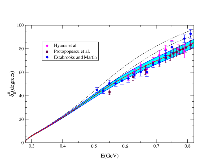
Figure 1: Isoscalar S-wave. The shaded band is taken from fig. 7 of CGL. The full line in the middle of the band represents the solution of the Roy equations obtained with the asymptotics of PY. For comparison, the representation proposed in eq. (5.4a) of PY is indicated by the dashed lines.

In order to determine the effect of the change in the asymptotics on the solutions of the Roy equations, we fix the scattering lengths as well as the phenomenological input for 0.8 GeV$\,<\,$E$\,<\,$1.42 GeV at our central values, so that the result can be compared with our central solution. Above 1.42 GeV, we evaluate the imaginary parts with the Regge representation of PY. The essential elements of the calculation are described in the appendices B and C. The result for $\delta_{0}^{0}$ is shown in fig. 1, where we compare the solution in eq. (C) with the band of solutions obtained in CGL. The graph shows that the low energy behaviour of $\delta^{0}_{0}$ is not sensitive to the input used in the region above 1.42 GeV – the distortion claimed in PY does not take place.

In PY, the “possible cause of the distortion of the CGL solution” is discussed in some detail and a low energy parametrization for the isoscalar S-wave is proposed, in support of that discussion. The proposal is referred to as a “tentative alternate solution” and is indicated by the dashed lines in fig. 1. As can be seen from this plot, the proposal is inconsistent both with our asymptotics and with the one of PY.

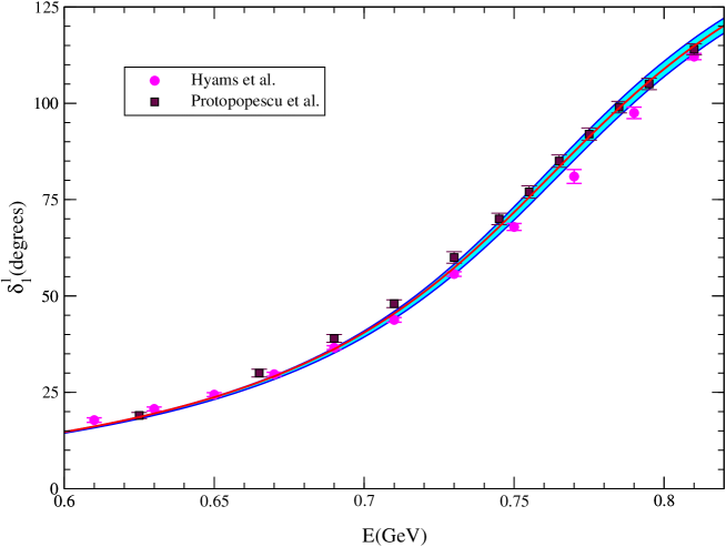
Figure 2: P-wave. The shaded band is taken from fig. 8 of CGL. The full line is the solution of the Roy equations obtained with the asymptotics of PY.

As a side remark, we note that on the interval on which we solve the Roy equations, the various phase shift analyses are not consistent with one another (see column 1 in table 2 of ACGL). For this reason, we did not make use of the data on the S- and P-wave phase shifts below 0.8 GeV – any analysis that relies on these is subject to large uncertainties. In contrast to the overall phase of the scattering amplitude, which is notoriously difficult to measure, the phase difference $\delta_{1}^{1}-\delta_{0}^{0}$ shows up directly in the cross section and is therefore known quite accurately. Indeed, the values obtained at 0.8 GeV from the seven different phase shift analyses listed in ACGL (which are due to Ochs [20], Hyams et al. [17], Estabrooks and Martin [21], Protopopescu et al. [22], Au et al. [23] and Bugg et al. [18]) yield perfectly consistent results for this phase difference: $\delta_{1}^{1}-\delta_{0}^{0}=26.6^{\circ}\pm 2.8^{\circ}$. While our Roy solutions agree with this experimental fact (no wonder, we are using it in our input), the ”tentative alternate solution” and the representation for the P-wave proposed in PY do not: These yield $\delta_{0}^{0}=91.9^{\circ}\pm 2.6^{\circ}$ and $\delta_{1}^{1}=109.0^{\circ}\pm 0.6^{\circ}$, respectively. The corresponding phase difference, $\delta_{1}^{1}-\delta_{0}^{0}=17.1^{\circ}\pm 2.6^{\circ}$, is in conflict with experiment at the level of 2.5 $\sigma$. The discrepancy must be blamed on the ”tentative alternate solution” – the uncertainties in the P-wave phase shift are small, because this phase is strongly constrained by the data on the form factor (indeed the value in PY is in good agreement with our estimate, $\delta_{1}^{1}=108.9^{\circ}\pm 2^{\circ}$).

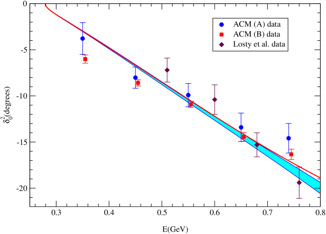
Figure 3: Exotic S-wave. The shaded band is taken from fig. 9 of CGL. The full line is the solution of the Roy equations obtained with the asymptotics of PY.

Fig. 2 demonstrates that the P-wave phase shift is not sensitive to the asymptotics, either. In the exotic S-wave (isospin 2), however, an effect does become visible. As can be seen in fig. 3, the modification of the asymptotic behaviour reduces the value of $\delta_{0}^{2}$. At 0.8 GeV, the displacement reaches $1.4^{\circ}$. Although this is small compared to the experimental uncertainties, it does imply that – if the imaginary parts above 1.42 GeV are taken from PY – the phase $\delta_{0}^{2}$ runs within our band of uncertainties only below 0.64 GeV.

5 Threshold parameters

Next, we evaluate the change occurring in the result for the scattering lengths and effective ranges of the lowest few partial waves if our asymptotics is replaced by the one of PY. The evaluation is based on sum rules due to Wanders [24], which are particularly suitable here, because they are rapidly convergent and thus not sensitive to the high energy behaviour of the imaginary parts. The representation for $a_{1}^{1}$, for instance, reads

$$a_{1}^{1} \!\!\!= \!\!\!\frac{2\,a_{0}^{0}-5\,a_{0}^{2}}{18\,M_{\pi}^{2}}+\frac{M_{\pi}^{2}}{36\,\pi^{2}}\int_{4M_{\pi}^{2}}^{\infty}\frac{ds}{s^{2}(s-4M_{\pi}^{2})^{2}}\left\{3\,(3\,s-4M_{\pi}^{2})\,\mbox{Im}\,T^{1}(s,0)\right.$$

$$\!\!\!\hskip 120.00018pt\left.-(s-4M_{\pi}^{2})(2\,\mbox{Im}\,T^{0}(s,0)-5\,\mbox{Im}\,T^{2}(s,0))\right\}\,.$$

	CGL	PY	units
$b_{0}^{0}$	$0.276\pm.006$	$\rule{3.00003pt}{0.0pt}0.278$	$M_{\pi}^{-2}$
$b_{0}^{2}$	$-0.803\pm.012$	$-0.800$	$10^{-1}M_{\pi}^{-2}$
$a_{1}^{1}$	$0.379\pm.005$	$0.381$	$10^{-1}M_{\pi}^{-2}$
$b_{1}^{1}$	$0.567\pm.013$	$0.579$	$10^{-2}M_{\pi}^{-4}$

Table 2: Wanders sum rules. The numbers in the first column are taken from table 2 of CGL. Those in the second column are obtained by replacing the asymptotics used there with the one proposed in PY.

The analogous sum rules for the effective ranges of the S- and P-waves are listed in appendix D. The numerical results of CGL are quoted in the first column of table 2, while those in the second column are obtained by repeating the calculation for the asymptotics proposed in PY. Note that the subtraction constants play a crucial role here. In fact, $a_{1}^{1}$ is totally dominated by the contribution from the first term on the right hand side of eq. (5), which accounts for 97 % of the numerical result. This is why the uncertainty in our prediction for $a_{1}^{1}$ is so small. The subtractions ensure that the integrals converge rapidly. For the asymptotics of PY, for instance, the contributions from the region above 1.42 GeV amount to less than 5% of the total, for all of the quantities listed in the table.

	Wanders		Froissart-Gribov
	CGL	PY	CGL	PY	units
$a^{0}_{2}$	$0.175\pm 0.003$	$0.180$	$0.176$	$0.180$	$10^{-2}M_{\pi}^{-4}$
$b_{2}^{0}$	$-0.355\pm 0.014$	$-0.347$	$-0.359$	$-0.353$	$10^{-3}M_{\pi}^{-6}$
$a^{2}_{2}$	$0.170\pm 0.013$	$0.177$	$0.172$	$0.182$	$10^{-3}M_{\pi}^{-4}$
$b_{2}^{2}$	$-0.326\pm 0.012$	$-0.327$	$-0.329$	$-0.319$	$10^{-3}M_{\pi}^{-6}$
$a_{3}^{1}$	$0.560\pm 0.019$	$0.562$	$0.560$	$0.565$	$10^{-4}M_{\pi}^{-6}$
$b_{3}^{1}$	$-0.402\pm 0.018$	$-0.409$	$-0.404\rule{5.0pt}{0.0pt}$	$-0.407$	$10^{-4}M_{\pi}^{-8}$

Table 3: Threshold parameters of the D- and F-waves. The left half of the table lists the results found with the analog of the Wanders sum rules, while the numbers on the right half are based on the Froissart-Gribov representation discussed in section 9. The results obtained with the asymptotics of CGL and of PY are listed separately. The first column is taken from table 2 of CGL.

Repeating the exercise for the D- and F-waves, we obtain the results listed on the left half of table 3. These indicate that the change in the asymptotics generates a somewhat larger effect, but the displacement stays below 5% also here. In the case of $a_{2}^{0}$, the shift corresponds to 1.5 $\sigma$, while for the other quantities the prediction is not that sharp, so that the shift is only a fraction of our error bar. In summary, we note that for none of the quantities considered in PY, the change in the asymptotics proposed in that paper generates a displacement by more than $1.5\,\sigma$.

There is an alternative method for evaluating the quantities listed in the table: Instead of working with the analog of the Wanders sum rules, we may invoke the Froissart-Gribov representation for the scattering lengths and effective ranges. The difference between the two is discussed in some detail in appendix D. If the scattering amplitude were exactly crossing symmetric, the two methods of calculation would yield identical results. The numerical results obtained with the FG-representation for the P- and D-waves are discussed in sections 7 and 9, respectively.

The entries in columns 1 and 3 show that, for our asymptotics, the two sets of numbers indeed agree within a fraction of a percent, indicating that our representation of the scattering amplitude does pass this test of crossing symmetry. The comparison of columns 2 and 4 indicates that the asymptotics of PY generates a somewhat stronger violation of crossing symmetry, but the differences do not stick out of the uncertainties that must be attached to the central values listed. As will be discussed in section 9, however, these differences originate in the tiny contributions from the asymptotic region and from the higher partial waves. In fact, the slight mismatch seen in the comparison of columns 2 and 4 implies that the asymptotics of PY is not consistent with crossing symmetry.

6 Olsson sum rule

We now turn to the calculations described in PY and start with the Olsson sum rule,

$$\!\!\!2\,a_{0}^{0}-5\,a_{0}^{2}=O\,,$$ (3)

which relates a combination of $S$-wave scattering lengths to an integral over the imaginary part of the forward scattering amplitude:

$$O=\frac{M_{\pi}^{2}}{8\pi^{2}}\int_{4M_{\pi}^{2}}^{\infty}\!ds\;\frac{2\,\mbox{Im}\,T^{0}(s,0)+3\,\mbox{Im}\,T^{1}(s,0)-5\,\mbox{Im}\,T^{2}(s,0)}{s\,(s-4M_{\pi}^{2})}\,.$$ (4)

It is well known that this integral converges only slowly – in contrast to the subtracted dispersion integrals that underly the Roy equations or the sum rule for the P-wave scattering length considered above, the contributions from the asymptotic region play a significant role here.

In ACGL, we evaluated the integral for arbitrary values of the S-wave scattering lengths. Inserting the predictions obtained on the basis of chiral symmetry in eq. (11.2) of that paper and accounting for the correlation between $a_{0}^{0}$ and $a_{0}^{2}$ with table 4 of CGL, we obtain $O_{\mbox{\tiny CGL}}=0.665\pm 0.022$. Since this is in perfect agreement with our prediction for the scattering lengths, $2a_{0}^{0}-5a_{0}^{2}=0.663\pm 0.007$, we conclude that, for our asymptotics, the Olsson sum rule is in equilibrium.

Peláez and Ynduráin point out that if our asymptotics is replaced by theirs, while the behaviour below 0.82 GeV is left unchanged, the value of the integral is reduced to $O_{\mbox{\tiny PY}}=0.635\pm 0.014$, so that the sum rule gets out of equilibrium. The low energy part of their calculation is examined in appendix E, where we essentially confirm their result. Using their numbers for the contributions from the region above 0.82 GeV, we find that the difference $\Delta=2a_{0}^{0}-5a_{0}^{2}-O$ between the left and right hand sides of the sum rule becomes $\Delta=0.025\pm 0.013$, a discrepancy of about $2\,\sigma$ (see the detailed discussion in appendix E).

The result implies that the following three statements are incompatible: (i) the behaviour of the phases below 0.8 GeV is correctly described by the figures shown above, (ii) the contributions above 0.8 GeV are correctly estimated in PY, (iii) the theoretical prediction for $2a_{0}^{0}-5a_{0}^{2}$ is valid. In PY, the blame is put on (i). The Roy equation analysis described in section 4, however, shows that (i) can only fail if either (ii) or (iii) or both are incorrect as well. Since the phenomenological information leaves little room for modifications in the interval from 0.8 to 1.4 GeV, we conclude that the asymptotics proposed in PY is in conflict with the theoretical predictions for the S-wave scattering lengths.

7 Froissart-Gribov formula for the P-wave

In this section, we consider the Froissart-Gribov formula

$$a_{1}^{1}=\frac{1}{144\pi^{2}}\!\int_{4M_{\pi}^{2}}^{\infty}\frac{ds}{s^{2}}\left\{2\mbox{Im}\,T^{0}(s,4M_{\pi}^{2})+3\mbox{Im}\,T^{1}(s,4M_{\pi}^{2})-5\mbox{Im}\,T^{2}(s,4M_{\pi}^{2})\right\}\,,$$ (5)

which is used in PY to evaluate the P-wave scattering length. The main difference to the Wanders representation in eq. (5) is that the FG formula does not contain a subtraction term and therefore converges more slowly: While in the above formula, the region above 1.42 GeV is responsible for more than 20% of the total, only a fraction of a percent arises from there in the case of the Wanders sum rule. The contrast is even more pronounced in the case of $b_{1}^{1}$, where the low energy contributions nearly cancel, so that the result obtained on the basis of the FG formula is dominated by those from high energies: For the asymptotics of PY, 98% (78%) of the total come from the region above 1.42 GeV (2 GeV). For this reason, the values found on the basis of the FG representation come with a large uncertainty. A numerical evaluation is of interest because it offers a test of the input used in the asymptotic region, but it does not add anything of significance to our knowledge of the values of $a_{1}^{1}$ and $b_{1}^{1}$. This is why, in table 2, we did not list the numerical values obtained in this way.

As both representations for $a_{1}^{1}$ are exact, the difference amounts to a sum rule, which the imaginary parts of the scattering amplitude must obey. Indeed, the integrand of the above representation is very similar to the one occurring in the Olsson sum rule (4) and the dominating contribution to the difference between the two representations is proportional to this sum rule. The remainder involves the sum rule derived in appendix C of ACGL. As shown there, the absence of a Pomeron contribution to the $I_{t}=1$ amplitude and crossing symmetry imply that the integral

$$\!\!\!S(t)\equiv\int_{4M_{\pi}^{2}}^{\infty}\!\frac{ds\,f(s,t)}{(s+t-4M_{\pi}^{2})}$$ (6)

$$\!\!\!\rule{0.0pt}{22.0pt}f(s,t)=\frac{2\,\mbox{Im}\,\bar{T}^{0}(s,t)+3\,\mbox{Im}\,\bar{T}^{1}(s,t)-5\,\mbox{Im}\,\bar{T}^{2}(s,t)}{12\,s}-\frac{(s-2M_{\pi}^{2})\,\mbox{Im}\,T^{1}(s,0)}{s\,(s-4M_{\pi}^{2})\,(s-t)}$$

must vanish in the entire region where the fixed-$t$ dispersion relations are valid. Crossing symmetry does not impose a constraint on the imaginary parts of the S-waves – indeed, these drop out on the right hand side of eq. (6). Hence the sum rule $S(t)=0$ relates a family of integrals over the imaginary part of the P-wave to the higher partial waves. The difference between the Froissart-Gribov and Wanders representations for $a_{1}^{1}$ may be written as a linear combination of the Olsson sum rule and the value of $S(t)$ at $t=4M_{\pi}^{2}$:

$$\!\!\!a_{1}^{1}\,\rule[-5.0pt]{0.20004pt}{13.00005pt}_{\,\mbox{\tiny FG}}-a_{1}^{1}\,\rule[-5.0pt]{0.20004pt}{13.00005pt}_{\,\mbox{\tiny W}}=-\frac{1}{18M_{\pi}^{2}}(2\,a_{0}^{0}-5\,a_{0}^{2}-O)+\frac{M_{\pi}^{2}}{3\pi^{2}}\,S(4M_{\pi}^{2})\,.$$ (7)

There is an analogous formula also for $b_{1}^{1}$:

$$b_{1}^{1}\,\rule[-5.0pt]{0.20004pt}{13.00005pt}_{\,\mbox{\tiny FG}}-b_{1}^{1}\,\rule[-5.0pt]{0.20004pt}{13.00005pt}_{\,\mbox{\tiny W}}=\frac{1}{3\pi^{2}}\,\frac{\partial}{\partial t}\{t\,S(t)\}\,\rule[-10.00002pt]{0.20004pt}{20.00003pt}_{\;t\rightarrow 4M_{\pi}^{2}}\,.$$ (8)

Note that this relation involves the derivative with respect to $t$, because the FG representation for $b_{1}^{1}$ contains the imaginary part as well as the first derivative thereof (see appendix D).

The difference between the FG and W representations for $a_{1}^{1}$ and $b_{1}^{1}$ reflects the fact that the former is derived from an unsubtracted dispersion relation, while the latter is based on the standard, subtracted form. If we wish, we may just as well apply the FG projection to the standard form of the fixed-$t$ dispersion relations. The procedure leads to a representation that also holds for the S-waves. In fact, the resulting formulae for $b_{0}^{0}$, $b_{0}^{2}$, $a_{1}^{1}$ and $b_{1}^{1}$ coincide with the Wanders sum rules. In this sense, the difference between the Froissart-Gribov and Wanders representations for the quantities considered above exclusively concerns the manner in which the contributions from the subtractions are dealt with. For the threshold parameters of the higher waves, on the other hand, the subtractions do not make any difference.

In the units of table 2, the numerical evaluation of the integrals yields

$$\!\!\!a_{1}^{1}\,\rule[-5.0pt]{0.20004pt}{13.00005pt}_{\,\mbox{\tiny FG}}\simeq 0.37\hskip 20.00003ptb_{1}^{1}\,\rule[-5.0pt]{0.20004pt}{13.00005pt}_{\,\mbox{\tiny FG}}\simeq 0.37\hskip 20.00003pt\mbox{(CGL)}\,,$$ (9)

$$\!\!\!a_{1}^{1}\,\rule[-5.0pt]{0.20004pt}{13.00005pt}_{\,\mbox{\tiny FG}}\simeq 0.36\hskip 20.00003ptb_{1}^{1}\,\rule[-5.0pt]{0.20004pt}{13.00005pt}_{\,\mbox{\tiny FG}}\simeq 0.56\hskip 20.00003pt\mbox{(PY)}\,.$$

The second line confirms the central values given in PY: $a_{1}^{1}\,\rule[-5.0pt]{0.20004pt}{13.00005pt}_{\,\mbox{\tiny FG}}=0.371\pm 0.013$, $b_{1}^{1}\,\rule[-5.0pt]{0.20004pt}{13.00005pt}_{\,\mbox{\tiny FG}}=0.599\pm 0.088$ (the term “direct” used in that paper refers to the results obtained on the basis of the Wanders sum rules).

The above numbers show that, irrespective of the asymptotic input used, the estimates obtained for $a_{1}^{1}$ on the basis of the FG formula are in reasonable agreement with the much more precise result found with the Wanders sum rule (see table 2). The number extracted from the FG representation for $b_{1}^{1}$, however, is reasonably close to the truth only for the asymptotics of PY.

As mentioned above, the FG integral for $b_{1}^{1}$ is dominated by the contributions from high energies. More precisely, the Regge term with the quantum numbers of the $\rho$ is relevant, for which we are using a parametrization of the form $\beta_{\rho}(t)s^{\alpha_{0}+\alpha_{1}t}$. For the integrals discussed in CGL, the uncertainty in the contribution from this term is governed by the one in the residue $\beta_{\rho}(t)$, but this is not the case here: Since the FG integral for $b_{1}^{1}$ converges only very slowly, it is very sensitive also to the parameters that describe the trajectory. While the values $\alpha_{0}=\frac{1}{2}-\alpha_{1}\,M_{\pi}^{2}\simeq 0.49$, $\alpha_{1}=\frac{1}{2}(M_{\rho}^{2}-M_{\pi}^{2})^{-1}\simeq 0.87\,\mbox{GeV}^{-2}$ used in CGL are determined by $M_{\rho}$ and $M_{\pi}$, those in PY, $\alpha_{0}=0.52\pm 0.02$, $\alpha_{1}=1.01\,\mbox{GeV}^{-2}$, are based on fits to cross sections. In the case of the Wanders representation for $b_{1}^{1}$, the change occurring if the trajectory used in CGL is replaced by the one in PY is small compared to the error in our result, $b_{1}^{1}=0.567\pm 0.013$, but in the case of the Froissart-Gribov representation, the operation shifts the outcome from 0.37 to 0.45 $(\alpha_{0}=0.50)$ or 0.53 ($\alpha_{0}=0.54$). Furthermore, the uncertainty attached to the Regge residue in CGL affects the result at the level of $\pm 0.06$. Note also that the FG-representation involves a derivative with respect to $t$, so that not only the slope $\alpha_{1}$ of the trajectory enters, but also the slope of the residue $\beta_{\rho}(t)$. Both of these quantities are poorly known.

We conclude that the FG-value for $b_{1}^{1}$ obtained with our asymptotics is subject to a large uncertainty, because it depends on minute details of the Regge representation: The discrepancy with the value found in CGL is in the noise. We repeat that the issue does not touch our prediction for $b_{1}^{1}$, for two reasons: (i) That prediction relies on the rapidly convergent representation of Wanders, where the entire region above 2 GeV contributes less than 2% of the total. (ii) The Wanders sum rule for $b_{1}^{1}$ does not involve derivatives with respect to $t$.

8 Values of $a_{1}^{1}$ and $b_{1}^{1}$ from $e^{+}e^{-}$ and $\tau$ data

The data on the pion form factor can be used to arrive at an independent determination of the P-wave parameters. As pointed out in PY, the numbers for $b_{1}^{1}$ obtained from fits based on the method of de Trocóniz and Ynduráin [25] disagree with our prediction at the $4\,\sigma$ level.

The partial wave parametrization used in ref. [25] is of inverse amplitude type:

$$t_{1}^{1}(s) \!\!\!= \!\!\!\left\{4\,\frac{M_{\rho}^{2}-s}{s-4M_{\pi}^{2}}\;(B_{0}+B_{1}\,z)-i\,\sqrt{1-\frac{4M_{\pi}^{2}}{s}}\right\}^{-1}\,,$$

$$z \!\!\!= \!\!\!\frac{\sqrt{s}-\sqrt{s_{1}-s}}{\sqrt{s}+\sqrt{s_{1}-s}}\,.$$ (10)

On the interval $4M_{\pi}^{2}<s<s_{1}$, the square roots are real, so that the expression obeys elastic unitarity. For $B_{1}=0$, the formula reduces to $\rho$–meson dominance. At $s=s_{1}$, the term $B_{1}\,z$ develops a branch cut that mimics contributions from inelastic channels. In PY, the value of $\sqrt{s_{1}}$ is fixed at 1.05 GeV, while $M_{\rho}$, $B_{0}$ and $B_{1}$ are treated as free parameters. Two of these specify the mass and the width of the $\rho$, while the third describes the behaviour near threshold, which is governed by the scattering length $a_{1}^{1}$. The authors use the above representation to evaluate the Omnès factor, which accounts for the branch cut singularity generated by the final state interaction. The remaining singularities, in particular also the branch cuts associated with inelastic channels, are parametrized in terms of a polynomial in a conformal variable that is adapted to the analytic structure of the form factor. The authors then make a fit to the $e^{+}e^{-}$ and $\tau$ data for energies below 0.96 GeV and come up with remarkably accurate values for the parameters $M_{\rho}$, $B_{0}$ and $B_{1}$. The corresponding result for the phase at 0.8 GeV is $\delta_{1}^{1}=109.0^{\circ}\pm 0.6^{\circ}$, while for scattering length and effective range, the threshold expansion of the above formula yields $a_{1}^{1}=(38.6\pm 1.2)\cdot 10^{-3}$ and $b_{1}^{1}=(4.47\pm 0.29)\cdot 10^{-3}$, respectively. Table 2 shows that the result for $a_{1}^{1}$ is consistent with our prediction, but the one for $b_{1}^{1}$ is not. It is evident from this table that the discrepancy cannot be blamed on the input used in the asymptotic region.

The problem with the above determination of $b_{1}^{1}$ is that it depends on the specific form of the parametrization used for the phase. To explicitly demonstrate this model–dependence, it suffices to allow for additional terms in the conformal polynomial, replacing $B_{0}+B_{1}z$ by $B_{0}+B_{1}z+B_{2}z^{2}+B_{3}z^{3}$. For simplicity, let us fix $a_{1}^{1}$ as well as $b_{1}^{1}$ at the central values obtained in CGL. We can choose the remaining three parameters in such a way that the phase stays close to the one specified in eq. (3.5) of PY. With $M_{\rho}=773.6\,\mbox{GeV}$, $B_{0}=1.073$, $B_{1}=0.214$, $B_{2}=-0.039$, $B_{3}=-0.267$, for instance, the scattering length as well as the effective range agree with the central values in CGL and the phase stays well within the uncertainty band that follows from the errors attached to the parameters in PY (despite the fact that these cannot be taken literally – above 0.82 GeV, the corresponding uncertainty in the phase is less than half a degree). Since the available experimental information does not strongly constrain the behaviour of the form factor in the threshold region, it is not possible to distinguish the two representations for the phase shift on phenomenological grounds.

Incidentally, one may also attempt to solve the Roy equations using the parametrization in eq. (8). The result is the same: Three parameters do not suffice to obtain solutions that obey the Roy equation for the P-wave, but with the above extension, the problem disappears. We conclude that the claimed 4 $\sigma$ discrepancy is a property of the model used to parametrize the P-wave phase shift and does not occur if one allows for the number of degrees of freedom necessary to trust the representation, not only for $a_{1}^{1}$, but also for $b_{1}^{1}$.

In connection with the contribution from hadronic vacuum polarization to the magnetic moment of the muon, we are currently performing an analysis of the form factor that is very similar to the one in ref. [25]. The main difference is that we do not invoke a parametrization in terms of a modified Breit-Wigner formula to describe the behaviour of the P-wave in the low energy region, but instead rely on the CGL phase shift [4]. We obtain a perfect description of the available experimental information about the form factor in this way, including the data in the spacelike region and we have checked that this also holds if we restrict our analysis to the data sets used in [25]. By construction, our parametrization of the form factor keeps the low energy parameters $a_{1}^{1}$ and $b_{1}^{1}$ fixed at the CGL values. This confirms the conclusion reached above: The experimental information on the form factor does not allow a model–independent determination of $a_{1}^{1}$ and $b_{1}^{1}$ at the level of accuracy claimed in PY.

9 Froissart-Gribov formula for the D-waves

Finally, we comment on the estimates for the threshold parameters of the D-waves given in PY. Using the Froissart–Gribov representation in eq. (D.8), the authors arrive at values for the combinations $a_{0+}=\frac{2}{3}(a_{2}^{0}-a_{2}^{2})$ and $a_{00}=\frac{2}{3}(a_{2}^{0}+2\,a_{2}^{2})$ that differ from those obtained with the results of CGL by about 4%. They then argue that the two evaluations are correlated and come up with the conclusion that, if the correlations are accounted for, this difference amounts to a discrepancy of 4 $\sigma$ in the case of $a_{0+}$ and 5 $\sigma$ in the case of $a_{00}$.

The main observation concerning the comparison is that it does not allow one to draw any conclusions about the S- and P-waves, because the contributions from these waves are identical in the two evaluations. When the correlations are accounted for, these contributions drop out in the comparison. For this reason, the differences discussed in PY between the “CGL–direct” and their own calculation of the D-wave threshold parameters do not involve any of the results of CGL. Even if the discrepancies obtained in PY could be taken at face value, the only conclusion we could draw from these is that the Regge representation proposed in PY differs from the one used in CGL – but this is evident ab initio. The situation for the Olsson sum rule and the P-wave threshold parameters is different: In those cases, the contributions from the S- and P-waves do not drop out, so that the CGL analysis does enter the comparison.

Moreover, for the D-wave threshold parameters, PY do not refer to (and we are not aware of) a determination that is independent of the sum rules. If this were available, one could use it, together with the assumption that the asymptotics of PY is correct, to draw conclusions about the size of the contributions from the low-energy region and decide whether the results obtained in CGL are consistent with those conclusions. This is the logic the authors follow with the Olsson sum rule, where they can use the low–energy theorem, and with the P-wave threshold parameters, where PY claim that fits to the data on the form factor allow one to determine $a_{1}^{1}$ and $b_{1}^{1}$ more reliably than with the sum rule (in section 8 we explained why this is not the case). For the D-wave threshold parameters, however, an analogous claim is not made. Hence the comparison of the results obtained by inserting the two different representations for the asymptotic region and for the higher partial waves in the integrals for the threshold parameters cannot possibly lead to conclusions that go beyond the fact that those two representations are different.

The FG integral converges almost as rapidly as the Wanders representation – the region above 1.42 GeV only contributes a small fraction of the total. For this reason, table 3 also lists the results obtained with the Froissart-Gribov representation. The requirement that the two different expressions for the D- and F-waves must lead to the same result amounts to a set of sum rules, which exclusively involve the imaginary parts of the higher partial waves. The prototype of this category of sum rules is the one in eq. (B.7) of ACGL. Since a crossing symmetric scattering amplitude automatically obeys these relations, they amount to a test of crossing symmetry. The sum rules require the contributions from the region below 1.42 GeV to be in balance with those from higher energies. Since the low energy part is dominated by the experimentally well determined isoscalar D-wave, the sum rules amount to a test of the representation for the imaginary parts used in the asymptotic region (which contain $I_{t}=0$ contributions from the Pomeron and $f$ poles, as well as poorly known terms with $I_{t}=2$). In application to PY, this test does not involve anything beyond the parametrizations proposed in that reference for the partial waves with $\ell\geq 2$ and for the asymptotic region. For the central values of the parameters, the difference between the results obtained from the Froissart-Gribov and Wanders representations becomes (in the normalization used for the D-waves in PY: scattering lengths in units of $10^{-4}\,M_{\pi}^{-4}$, effective ranges in units of $10^{-4}\,M_{\pi}^{-6}$):

$$\Delta a_{0+}^{\mathrm{PY}}=-0.11\;\;,\quad\Delta a_{00}^{\mathrm{PY}}=0.03\;\;,\quad\Delta b_{0+}^{\mathrm{PY}}=-0.13\;\;,\quad\Delta b_{00}^{\mathrm{PY}}=0.09\;\;.$$

These numbers show that – for the parametrizations proposed in PY – the two representations do not lead to the same result, so that there is an inherent uncertainty in the values obtained for the D-wave threshold parameters. In fact, with the exception of $a_{00}$, the above numbers are all larger than the uncertainties quoted in PY for the discrepancy between “CGL–direct” and their own evaluation. Evidently, those uncertainties are underestimated. In terms of the error attached to the comparison of the values obtained for $b_{0+}$, for instance, their asymptotics violates crossing symmetry at the level of 5 $\sigma$. In other words, their Regge parametrization is not in equilibrium with the low energy structure: The various terms from the asymptotic region roughly cancel, so that almost nothing is left to compensate the contribution from the f₂(1275), which dominates the low energy part of the integral.

The problem does not occur with our asymptotics, for which the sum rules hold to a remarkable degree of accuracy: with the central values of our parameters we get

$$\Delta a_{0+}^{\mathrm{CGL}}=-0.006\;\;,\quad\Delta a_{00}^{\mathrm{CGL}}=-0.009\;\;,\quad\Delta b_{0+}^{\mathrm{CGL}}=-0.007\;\;,\quad\Delta b_{00}^{\mathrm{CGL}}=-0.03\;\;.$$

In PY, it is stated that the discrepancies obtained with the Froissart-Gribov formula for the effective ranges cannot be taken as seriously as those for the scattering lengths, because the result is sensitive to the $t$-dependence of the $I_{t}=2$ exchange piece. The violation of crossing symmetry, however, also shows up in the scattering lengths: For the parametrization proposed in PY, the net asymptotic contribution to $\Delta a_{0+}$, for instance, is also much too small to keep the term from the $f_{2}(1275)$ in balance, while for $\Delta a_{00}$, it is much too large.

Note that the sum rules receive contributions exclusively from (a) the Regge representation and (b) the low energy parametrization used for the higher partial waves. Both of these contributions are small in comparison to the net result for the threshold parameters, because that result is dominated by the contributions from the S- and P-waves. For the test of crossing symmetry, however, this comparison is of no significance, because the S- and P-waves do not contribute at all. What counts is whether or not (a) is in equilibrium with (b).

We conclude that, while the asymptotics used in CGL is consistent with crossing symmetry, the one proposed in PY is not. The violation is too large for the comparison with CGL to be meaningful at the level of accuracy claimed in PY.

10 Summary and conclusions

The low energy analysis of the $\pi\pi$ scattering amplitude described in CGL relies on input for the imaginary parts, which are partly taken from experiment, partly from Regge theory. In the present paper, we have investigated the sensitivity of the results to the input used in the asymptotic region. The investigation is motivated by a recent paper of Peláez and Ynduráin, who advise the reader not to trust the results of CGL, because in their opinion, the input used for the asymptotics is wrong.

The Regge representation of CGL is based on the work of Pennington and Protopopescu [11] and is indeed quite different from the one proposed in PY. The main result of the analysis described in the first part of the present article is that – as far as the low energy behaviour of the scattering amplitude is concerned – this difference does not matter. The input used for the imaginary parts above 1.42 GeV may be replaced by the one advocated in PY. The outcome for the threshold parameters of the leading partial waves remains almost the same:

• The predictions for the S-wave scattering lengths are practically untouched. Expressed in terms of the uncertainty estimates given in CGL, the changes amount to less than 0.15 $\sigma$. This is of crucial importance, because the result implies that the subtraction constants in the fixed-$t$ dispersion relations stay put – the subtraction constants are the essential parameters in the low energy domain.

• Neither the effective ranges of the S-waves nor the threshold parameters of the P-wave are sensitive to the input used in the asymptotic region. The effects seen in the higher partial waves are somewhat larger, but the only case where replacing the asymptotics of CGL by the one of PY produces a change that exceeds our error estimates is the isoscalar D-wave scattering length $a_{2}^{0}$, where the displacement amounts to 1.5 $\sigma$.

• The Roy equations imply that the low energy behaviour of the isoscalar S-wave and the P-wave remains practically unaffected by the change in the asymptotics (see figs. 1 and 2). The exotic S-wave (isospin 2) is more sensitive, but even in that case, we find that the phase shift at 0.8 GeV is displaced by only $1.4^{\circ}$ (see fig. 3). As witnessed by the fact that the changes in $a_{0}^{2}$ and $b_{0}^{2}$ are minute, the behaviour in the threshold region essentially stays put also for this partial wave.

The calculation confirms the stability of our results with respect to the uncertainties in the asymptotic region. Even if the representation proposed in PY is assumed to be closer to the truth than the one of Pennington and Protopopescu that we rely on, the predictions for the threshold parameters remain essentially the same. We conclude that the statements made by Peláez and Ynduráin about the precision of chiral-dispersive calculations of $\pi\pi$ scattering are incorrect.

In the second part of the present article, we have examined the calculations described in PY. The main points to notice here are: (i) these do not shed any light on the values of the threshold parameters and (ii) the Regge parametrization proposed in PY cannot be valid within the uncertainties quoted for the parameters, because it violates crossing symmetry. Our asymptotic representation does not have this problem.

• In the case of the Olsson sum rule or the Froissart-Gribov representation for $a_{1}^{1}$, the integrals only converge slowly, so that the result is sensitive to the uncertainties in the imaginary parts above 1.4 GeV. In effect, the calculation yields a crude estimate for the combination $2\,a_{0}^{0}-5\,a_{0}^{2}$ of subtraction constants. The comparison with the very precise prediction obtained in ref. [2] shows that the asymptotic representation proposed in PY brings the Olsson sum rule out of equilibrium, while the one used in CGL passes the test very well. We conclude that the Regge representation proposed in PY is not consistent with the prediction of standard chiral perturbation theory for $2\,a_{0}^{0}-5\,a_{0}^{2}$.

• In the case of $b_{1}^{1}$, the Froissart-Gribov formula converges only very slowly, so that the result is sensitive to the behaviour of the imaginary parts at very high energies, in marked contrast to the integrals considered in CGL, where energies above 3 GeV barely contribute. For the central parameter values of the asymptotic representation used in CGL, the FG integral for $b_{1}^{1}$ comes out too small. The result, however, very strongly depends on details of the parametrization used for the Regge term with the quantum numbers of the $\rho$, so that there is no discrepancy to speak of.

• In PY, the method of ref. [25] is used to arrive at an independent determination of $a_{1}^{1}$ and $b_{1}^{1}$, based on the $e^{+}e^{-}$ and $\tau$ data. While the result for $a_{1}^{1}$ is in good agreement with our prediction, the value for $b_{1}^{1}$ is not. We show that the uncertainties attached to this method are underestimated. The data on the form factor are perfectly consistent with our predictions, not only for $a_{1}^{1}$, but also for $b_{1}^{1}$.

• The Froissart-Gribov representation for the threshold parameters of the D-waves converges about equally well as the Wanders representation used in CGL – in either case, the low energy region dominates. In PY, the difference between these two types of representation is used to test our results for the low energy region. Actually, however, the contributions from the S- and P-waves are identical in the two cases: A change in these waves shifts our results by exactly the same amount as theirs. Even if the discrepancies obtained in PY could be taken at face value, the only conclusion we could draw from the comparison of the numbers for the threshold parameters of the D-waves is that the asymptotic representation proposed in PY differs from the one used in CGL – but this is evident ab initio.

• The asymptotics proposed in PY violates crossing symmetry rather strongly, while for the one used in CGL, the violations are in the noise. In the case of $b_{0+}$, for instance, the representation of PY implies a violation of crossing symmetry that is more than twice as large as the discrepancy with our result that the authors are claiming. This shows that (i) their Regge representation cannot be valid down to 1.42 GeV and (ii) the uncertainties are underestimated, particularly those attached to the discrepancies obtained when comparing their results with ours.

There is no doubt that the representation used in CGL for the asymptotic region, as well as the one for the low energy contributions from the D- and F-waves could be improved. In particular, the $t$-dependence of the imaginary parts is poorly known at high energies. An improved representation could be found by exploiting the various sum rules discussed in the present article and comparing the result with what can be extracted from the experimental information about the behaviour at high energies by invoking factorization. A better knowledge of the imaginary parts in the region above 0.8 GeV is of interest, for instance, in connection with the Standard Model prediction for the magnetic moment of the muon: Our investigation of the pion form factor [4] relies on an extension of the Roy equation analysis to higher energies, where the uncertainties in the asymptotic region are not entirely negligible. Concerning the behaviour in the threshold region, however, we do not expect this investigation to add much to what is known already.

Appendix A Asymptotic representation of PY

In the notation of ACGL, the Regge representation used in PY for the imaginary parts above 1.42 GeV reads

$$\mbox{Im}\,T^{0}(s,t) \!\!\!= \!\!\!\mbox{$\frac{1}{3}$}f_{0}(s,t)+f_{1}(s,t)+\mbox{$\frac{5}{3}$}\,f_{2}(s,t)+(t\leftrightarrow u)\,,$$

$$\mbox{Im}\,T^{1}(s,t) \!\!\!= \!\!\!\mbox{$\frac{1}{3}$}f_{0}(s,t)+\mbox{$\frac{1}{2}$}\,f_{1}(s,t)-\mbox{$\frac{5}{6}$}\,f_{2}(s,t)-(t\leftrightarrow u)\,,$$ (A.1)

$$\mbox{Im}\,T^{2}(s,t) \!\!\!= \!\!\!\mbox{$\frac{1}{3}$}f_{0}(s,t)-\mbox{$\frac{1}{2}$}\,f_{1}(s,t)+\mbox{$\frac{1}{6}$}\,f_{2}(s,t)+(t\leftrightarrow u)\,.$$

The functions occurring here are given by

$$f_{0}(s,t) \!\!\!= \!\!\!n\;\sigma_{P}\,\left\{1+k_{1}\,(\hat{s}/s)^{1/2}\right\}\,e^{b\,t}\,(s/\hat{s})^{\alpha_{P}(t)}\,,$$

$$f_{1}(s,t) \!\!\!= \!\!\!n\left\{1+k_{2}\,(\hat{s}/s)^{1/2}\right\}\,\,f(s,t)\,,$$

$$f_{2}(s,t) \!\!\!= \!\!\!n\,k_{4}\,f(s,t)^{2}\,(\hat{s}/s)\,,$$ (A.2)

$$f(s,t) \!\!\!= \!\!\!\,\sigma_{\rho}\,\frac{1+\alpha_{\rho}(t)}{1+\alpha_{\rho}(0)}\left\{(1+k_{3})\,e^{b\,t}-k_{3})\right\}(s/\hat{s})^{\alpha_{\rho}(t)}\,,$$

$$\alpha_{P}(t) \!\!\!= \!\!\!1+\alpha_{P}^{1}\,t\,,\rule{0.0pt}{11.99998pt}\hskip 20.00003pt\alpha_{\rho}(t)=\alpha_{\rho}^{0}+\alpha_{\rho}^{1}\,t\,.$$

The factor $n=4\,\pi^{2}$ accounts for the difference in normalization. The scale is fixed at $\hat{s}=1\,\mbox{GeV}^{2}$ and the various parameters are assigned the values

$$\alpha_{P}^{1} \!\!\!= \!\!\!0.11\pm 0.03\,\mbox{GeV}^{-2}\,,\hskip 20.00003pt\alpha_{\rho}^{0}=0.52\pm 0.02\,,\hskip 20.00003pt\alpha_{\rho}^{1}=1.01\,\mbox{GeV}^{-2}\,,$$

$$\sigma_{P} \!\!\!= \!\!\!3.0\pm 0.3\,,\hskip 20.00003pt\sigma_{\rho}=0.85\pm 0.10\,,\hskip 20.00003ptb=2.38\pm 0.20\,\mbox{GeV}^{-2}\,,$$ (A.3)

$$k_{1} \!\!\!= \!\!\!0.24\,,\hskip 10.00002ptk_{2}=0.4\pm 0.1\,,\hskip 10.00002ptk_{3}=1.48\,,\hskip 10.00002ptk_{4}=0.8\pm 0.2\,.$$

The value of $\sigma_{P}$ corresponds to an asymptotic cross section of $n\hskip 0.70007pt\sigma_{P}/3\hskip 0.70007pt\hat{s}\simeq 15\,\mbox{mb}$.

Appendix B Driving terms for asymptotics of PY

The contributions to the Roy equations that arise from the imaginary parts of the higher partial waves ($\ell\geq 2$) and from the high energy end of the dispersion integrals are referred to as driving terms. We evaluate the former as described in detail in ACGL, except that the integrals are now cut off at 1.42 GeV. Concerning the latter, we merely have to replace the Regge representation used in ACGL by the one of PY and take the lower limit of the integral over the energy at 1.42 GeV instead of 2 GeV. The result is well approximated by polynomials in $q^{2}=\frac{1}{4}(s-4M_{\pi}^{2})$:

$$d^{0}_{0}(s)_{\mbox{\tiny PY}} \!\!\!= \!\!\!0.16\,q^{2}+5.5\,q^{4}-6.6\,q^{6}+7.5\,q^{8}\,,$$

$$d^{1}_{1}(s)_{\mbox{\tiny PY}} \!\!\!= \!\!\!0.0011\,q^{2}+0.52\,q^{4}+0.13\,q^{6}+1.1\,q^{8}\,,$$ (B.1)

$$d^{2}_{0}(s)_{\mbox{\tiny PY}} \!\!\!= \!\!\!0.074\,q^{2}+2.7\,q^{4}-7.0\,q^{6}+8.8\,q^{8}\,,$$

where $q$ is taken in GeV units. The corresponding Roy equations are obtained by inserting these expressions in eqs. (5.1), (5.2) of ACGL, with $s_{0}=(0.8\,\mbox{GeV})^{2}$, $s_{2}=(1.42\,\mbox{GeV})^{2}$.

Appendix C Roy solution for asymptotics of PY

In order to study the effect of the change in the asymptotics on the solutions of the Roy equations, we fix the subtraction constants at $a_{0}^{0}=0.22$, $a_{0}^{2}=-0.0444$ and use our central values for the phenomenological input below 1.42 GeV, which are characterized by $\delta_{0}^{0}(s_{0})=82.0^{\circ}$, $\delta_{1}^{1}(s_{0})=108.9^{\circ}$. We describe the phases with a parametrization of the form

$$\tan\delta_{\ell}^{I}=\sqrt{1-{4M_{\pi}^{2}\over s}}\;q^{2\ell}\left\{A^{I}_{\ell}+B^{I}_{\ell}q^{2}+C^{I}_{\ell}q^{4}+D^{I}_{\ell}q^{6}\right\}\left({4M_{\pi}^{2}-s^{I}_{\ell}\over s-s^{I}_{\ell}}\right)\;.$$ (C.1)

Using the driving terms in eq. (B), we then obtain the following solution of the Roy equations (here, all quantities are given in units of $M_{\pi}$):

$$A_{0}^{0} \!\!\!= \!\!\!.220\,,\hskip 45.00006ptA^{1}_{1}=.380\cdot 10^{-1}\,,\hskip 22.0ptA^{2}_{0}=-.0444\,,$$

$$B_{0}^{0} \!\!\!= \!\!\!.269\,,\hskip 45.00006ptB^{1}_{1}=.144\cdot 10^{-3}\,,\hskip 20.00003ptB^{2}_{0}=-.936\cdot 10^{-1}\,,$$

$$C_{0}^{0} \!\!\!= \!\!\!-.137\cdot 10^{-1}\,,\hskip 10.00002ptC^{1}_{1}=-.719\cdot 10^{-4}\,,\hskip 13.00005ptC^{2}_{0}=-.119\cdot 10^{-1}\,,$$ (C.2)

$$D_{0}^{0} \!\!\!= \!\!\!-.146\cdot 10^{-2}\,,\hskip 10.00002ptD^{1}_{1}=-.117\cdot 10^{-5}\,,\hskip 11.99998ptD^{2}_{0}=.415\cdot 10^{-3}\,,$$

$$s^{0}_{0} \!\!\!= \!\!\!36.73\,,\hskip 44.0pts_{1}^{1}=30.70\,,\hskip 45.00006pts^{2}_{0}=-8.84\,.$$

Appendix D Representations for the threshold parameters

Subtractions

As discussed in the text, the subtractions play a central role in the low energy analysis. The fixed-$t$ dispersion relations are needed in order to derive the various representations for the threshold parameters used in the text. We first write these relations down explicitly.

If the subtractions are ignored, the fixed-$t$ dispersion relations are very simple:

$$\vec{T}(s,t)=\int_{4M_{\pi}^{2}}^{\infty}ds^{\prime}\left\{\frac{\mbox{Im}\,\vec{T}(s^{\prime},t)}{(s^{\prime}-s)}+\frac{C_{su}\cdot\mbox{Im}\,\vec{T}(s^{\prime},t)}{(s^{\prime}-u)}\right\}\,,$$ (D.1)

where $\vec{T}(s,t)=\{\vec{T}^{0}(s,t),\vec{T}^{1}(s,t),\vec{T}^{2}(s,t)\}$ is the vector formed with the three $s$-channel isospin components and $C_{su}$ is the $3\times 3$ crossing matrix relevant for $s\leftrightarrow u$. The dispersion integral diverges, however. In order to remove the divergent piece, a subtraction term of the form $\vec{c}_{0}(t)+s\,\vec{c}_{1}(t)$ is needed. As shown by Roy [5], crossing symmetry implies that the subtraction functions $\vec{c}_{0}(t)$ and $\vec{c}_{1}(t)$ are fully determined by the imaginary parts of the forward scattering amplitude, except for two constants. The dispersion relations then take the form

$$\vec{T}(s,t) \!\!\!= \!\!\!(4M_{\pi}^{2})^{-1}\,(s\,{\bf 1}+t\,C_{st}+u\,C_{su})\cdot\vec{T}(4M_{\pi}^{2},0)$$

$$\!\!\!+\int_{4M_{\pi}^{2}}^{\infty}\!ds^{\prime}\,g_{2}(s,t,s^{\prime})\cdot\mbox{Im}\,\vec{T}(s^{\prime},0)+\int_{4M_{\pi}^{2}}^{\infty}\!ds^{\prime}\,g_{3}(s,t,s^{\prime})\cdot\mbox{Im}\,\vec{T}(s^{\prime},t)\,.$$

The first term is fixed by the $S$-wave scattering lengths:

$$\vec{T}(4M_{\pi}^{2},0)=32\,\pi\,(a_{0}^{0},0,a_{0}^{2})\,.$$

The quantities $g_{2}$ and $g_{3}$ are built with the crossing matrices $C_{st}$, $C_{tu}$ and $C_{su}$:

$$g_{2}(s,t,s^{\prime}) = -\frac{t}{\pi\,s^{\prime}\,(s^{\prime}-4M_{\pi}^{2})}\,(u\,C_{st}+s\,C_{st}\,C_{tu})\left(\frac{{\bf 1}}{s^{\prime}-t}+\frac{C_{su}}{s^{\prime}-u_{0}}\right)\,,$$

$$g_{3}(s,t,s^{\prime}) = -\frac{s\,u}{\pi\,s^{\prime}(s^{\prime}-u_{0})}\left(\frac{{\bf 1}}{s^{\prime}-s}+\frac{C_{su}}{s^{\prime}-u}\right)\,,$$ (D.3)

with $u=4M_{\pi}^{2}-s-t$ and $u_{0}=4M_{\pi}^{2}-t$. One readily checks that the difference between the right hand sides of eqs. (D.1) and (D) is linear in $s$.

The scattering amplitude is invariant under the crossing operations $s\leftrightarrow t$, $s\leftrightarrow u$ and $t\leftrightarrow u$: $\vec{T}(s,t)=C_{tu}\cdot\vec{T}(s,u)=C_{st}\cdot\vec{T}(t,s)=C_{su}\cdot\vec{T}(u,t)$. These relations impose constraints on the imaginary part of the amplitude, which can be expressed in the form of sum rules [26, 27, 28]. In particular, inserting the dispersion relation (D) on the two sides of the equation

$$\vec{T}(s,t)=C_{st}\cdot\vec{T}(t,s)\,,$$ (D.4)

one obtains an entire family of such sum rules. Note that the relation $S(t)=0$, which we made use of in section 7, was considered long ago and was exploited to study the $t$-dependence of the residue of the Regge pole with the quantum numbers of the $\rho$ [28]. For a detailed discussion, we refer to [12].

Wanders representation

The threshold parameters are the coefficients occurring in the expansion of the scattering amplitude around the point $s=4M_{\pi}^{2}$, $t=0$. Setting

$$s=4\,(M_{\pi}^{2}+q^{2})\,,\hskip 20.00003ptt=-2\,q^{2}\,(1-z)\,.$$ (D.5)

and performing the expansion in powers of $q$ in the integrands on the right hand side of the dispersion relation (D), we arrive at the Wanders sum rules:

$$b_{0}^{0} \!\!\!= \!\!\!\frac{1}{3M_{\pi}^{2}}(2a_{0}^{0}-5a_{0}^{2})+\frac{M_{\pi}^{2}}{6\pi^{2}}\int_{4M_{\pi}^{2}}^{\infty}\frac{ds\,B_{0}^{0}(s)}{s^{2}(s-4M_{\pi}^{2})^{2}}-\beta\,(a_{0}^{0})^{2}$$

$$b_{0}^{2} \!\!\!= \!\!\!-\frac{1}{6M_{\pi}^{2}}(2a_{0}^{0}-5a_{0}^{2})+\frac{M_{\pi}^{2}}{12\pi^{2}}\int_{4M_{\pi}^{2}}^{\infty}\frac{ds\,B_{0}^{2}(s)}{s^{2}(s-4M_{\pi}^{2})^{2}}-\beta\,(a_{0}^{2})^{2}$$

$$a_{1}^{1} \!\!\!= \!\!\!\frac{2\,a_{0}^{0}-5\,a_{0}^{2}}{18\,M_{\pi}^{2}}+\frac{M_{\pi}^{2}}{36\,\pi^{2}}\int_{4M_{\pi}^{2}}^{\infty}\frac{ds\,A_{1}^{1}(s)}{s^{2}(s-4M_{\pi}^{2})^{2}}$$ (D.6)

$$b_{1}^{1} \!\!\!= \!\!\!\frac{1}{36\pi^{2}}\int_{4M_{\pi}^{2}}^{\infty}\frac{ds\,B^{1}_{1}(s)}{s^{3}(s-4M_{\pi}^{2})^{3}}\,.$$

The integrands are given by

$$B_{0}^{0}(s) \!\!\!= \!\!\!4(s-M_{\pi}^{2})\mbox{Im}\,T^{0}(s,0)+(s-4M_{\pi}^{2})\{-3\mbox{Im}\,T^{1}(s,0)+5\mbox{Im}\,T^{2}(s,0)\}-\beta^{0}(s)\,,$$

$$B_{0}^{2}(s) \!\!\!= \!\!\!(s-4M_{\pi}^{2})\{2\mbox{Im}\,T^{0}(s,0)+3\mbox{Im}\,T^{1}(s,0)\}+(7s-4M_{\pi}^{2})\mbox{Im}\,T^{2}(s,0))-\beta^{2}(s)\,,$$

$$A_{1}^{1}(s) \!\!\!= \!\!\!3\,(3\,s-4M_{\pi}^{2})\,\mbox{Im}\,T^{1}(s,0)+(s-4M_{\pi}^{2})\{-2\,\mbox{Im}\,T^{0}(s,0)+5\,\mbox{Im}\,T^{2}(s,0)\}\,,$$

$$B_{1}^{1}(s) \!\!\!= \!\!\!3\,(3\,s^{3}-12M_{\pi}^{2}s^{2}+48M_{\pi}^{4}s-64M_{\pi}^{6})\,\mbox{Im}\,T^{1}(s,0)$$

$$\!\!\!+(s-4M_{\pi}^{2})^{3}\{-2\,\mbox{Im}\,T^{0}(s,0)+5\,\mbox{Im}\,T^{2}(s,0)\}\,.$$

For the S-wave effective ranges, the expansion can be interchanged with the integration only after removing the threshold singularity. This can be done by supplementing the integrand with a total derivative, which gives rise to extra terms in the expressions for $b_{0}^{0}$ and $b_{0}^{2}$:

$$\beta^{0}(s) \!\!\!= \!\!\!\frac{48\,\pi}{M_{\pi}^{2}}\,(a_{0}^{0})^{2}\,h(s)\,\theta(s_{c}-s)\,,\hskip 20.00003pt\beta^{2}(s)=\frac{96\,\pi}{M_{\pi}^{2}}\,(a_{0}^{2})^{2}\,h(s)\,\theta(s_{c}-s)\,,$$

$$\beta \!\!\!= \!\!\!\frac{8}{\pi}\int_{s_{c}}^{\infty}\frac{ds}{s^{2}(s-4M_{\pi}^{2})^{2}}\,h(s)\,,\hskip 20.00003pth(s)=(s-2M_{\pi}^{2})\sqrt{s(s-4M_{\pi}^{2})}\,.$$

By construction, the result is independent of $s_{c}$.

The corresponding representations for the threshold parameters of the higher waves are obtained in the same manner – we are referring to all of these as Wanders representations. The one for the D-wave scattering lengths, for instance, takes the form

$$a^{0}_{2} \!\!\!= \!\!\!\frac{1}{90\pi^{2}}\int_{4M_{\pi}^{2}}^{\infty}\frac{ds\,A_{2}^{0}(s)}{s^{3}(s-4M_{\pi}^{2})^{2}}+\frac{M_{\pi}^{2}}{45\pi^{2}}\int_{4M_{\pi}^{2}}\frac{ds\,\dot{A}^{0}_{2}(s)}{s^{2}(s-4M_{\pi}^{2})^{2}}$$ (D.7)

$$a^{2}_{2} \!\!\!= \!\!\!\frac{1}{180\pi^{2}}\int_{4M_{\pi}^{2}}^{\infty}\frac{ds\,A_{2}^{2}(s)}{s^{3}(s-4M_{\pi}^{2})^{2}}+\frac{M_{\pi}^{2}}{90\pi^{2}}\int_{4M_{\pi}^{2}}\frac{ds\,\dot{A}^{2}_{2}(s)}{s^{2}(s-4M_{\pi}^{2})^{2}}\,.$$

In this case, the integrands

$$A_{2}^{0}(s) \!\!\!= \!\!\!3\,(s^{2}+4M_{\pi}^{2}s-16M_{\pi}^{4})\,\mbox{Im}\,T^{1}(s,0)$$

$$\!\!\!+(s-4M_{\pi}^{2})^{2}\{\mbox{Im}\,T^{0}(s,0)+5\,\mbox{Im}\,T^{2}(s,0)\}\,,$$

$$\dot{A}_{2}^{0}(s) \!\!\!= \!\!\!4(s-M_{\pi}^{2})\mbox{Im}\,\dot{T}^{0}(s,0)+(s-4M_{\pi}^{2})\{-3\,\mbox{Im}\,\dot{T}^{1}(s,0)+5\,\mbox{Im}\dot{T}^{2}(s,0)\}\,,$$

$$A_{2}^{2}(s) \!\!\!= \!\!\!-3\,(s^{2}+4M_{\pi}^{2}s-16M_{\pi}^{4})\,\mbox{Im}\,T^{1}(s,0)$$

$$\!\!\!+(s-4M_{\pi}^{2})^{2}\{2\,\mbox{Im}\,T^{0}(s,0)+\,\mbox{Im}\,T^{2}(s,0)\}\,,$$

$$\dot{A}_{2}^{2}(s) \!\!\!= \!\!\!(s-4M_{\pi}^{2})\{2\,\mbox{Im}\,\dot{T}^{0}(s,0)+3\,\mbox{Im}\,\dot{T}^{1}(s,0)\}$$

$$\!\!\!+(7\,s-4M_{\pi}^{2})\,\mbox{Im}\,\dot{T}^{2}(s,0)\,,$$

involve the first derivative of the scattering amplitude with respect to $t$,

$$\dot{T}^{I}_{\ell}(s,t)\equiv\frac{\partial}{\partial t}T^{I}_{\ell}(s,t)$$

We do not list the analogous expressions for the D-wave effective ranges or for the F-wave scattering length. These are obtained with the same algorithm and involve up to two derivatives.

Froissart-Gribov representation

The crossing relation (D.4) connects the properties of the amplitude in the vicinity of threshold to those in the vicinity of the point $s=0$, $t=4M_{\pi}^{2}$. The Froissart-Gribov representation of the threshold parameters may be obtained by inserting the unsubtracted dispersion relation (D.1) in eq. (D.4) and expanding the result around $s=4M_{\pi}^{2}$, $t=0$. Instead of the Wanders sum rules, we now obtain

$$a_{\ell}^{I} \!\!\!= \!\!\!\frac{2^{\ell}\,\ell!}{16\,\pi^{2}\,(2\ell+1)!!}\;\int_{4M_{\pi}^{2}}^{\infty}ds\;\frac{\mbox{Im}\,T^{(I)}(s,4M_{\pi}^{2})}{s^{\,\ell+1}}\,,$$ (D.8)

$$b_{\ell}^{I} \!\!\!= \!\!\!\frac{2^{\ell}\,\ell!}{8\,\pi^{2}\,(2\ell+1)!!}\;\int_{4M_{\pi}^{2}}^{\infty}ds\;\frac{2\,s\,\mbox{Im}\,\dot{T}^{(I)}(s,4M_{\pi}^{2})-(\ell+1)\mbox{Im}\,T^{(I)}(s,4M_{\pi}^{2})}{s^{\,\ell+2}}$$

The quantities $T^{(0)}(s,t)$, $T^{(1)}(s,t)$ and $T^{(2)}(s,t)$ represent the $t$-channel isospin components of the scattering amplitude,

$$T^{(I)}(s,t)=\sum_{I^{\prime}}C_{st}^{II^{\prime}}\,T^{I^{\prime}}(s,t)$$ (D.9)

and $\dot{T}^{(I)}(s,t)$ stands for the derivative of $T^{(I)}(s,t)$ with respect to $t$.

In view of the occurrence of subtractions, the representation holds in this form only for $\ell\geq 1$. In order to arrive at a representation that also holds for the S-waves, it suffices to insert in eq. (D.4) the subtracted version (D) of the dispersion relation rather than the unsubtracted one. The subtractions are linear in $s$. After crossing, they become linear in $t$ and thus drop out in all waves except S and P. So the expressions for the threshold parameters remain the same for $\ell\geq 2$. On the other hand, the term containing the function $g_{3}(s,t,s^{\prime})$ in eq. (D) is proportional to $s\,u$. After crossing, this becomes $t\,u=4\,q^{4}(1-z^{2})$. So, the term does not contribute to the scattering lengths or effective ranges of the S- and P-waves. Hence the resulting representation for these exclusively contains the imaginary parts in the forward direction. In fact, the representation for $b_{0}^{0}$, $b_{0}^{2}$, $a_{1}^{1}$, $b_{1}^{1}$ that obtains in this manner is identical with the Wanders sum rules in eq. (D). The exercise shows that the lowest terms in the threshold expansion of the subtracted fixed-$t$ dispersion relations automatically respect crossing symmetry.

Sum rule related to $a_{2}^{0}$

As mentioned in the text, the contributions from the S- and P-waves to the FG and W representations of the D- and F-wave threshold parameters are identical. For $\Delta a_{2}^{0}=a_{2}^{0}\,\rule[-5.0pt]{0.20004pt}{13.00005pt}_{\,\mbox{\tiny FG}}-a_{2}^{0}\,\rule[-5.0pt]{0.20004pt}{13.00005pt}_{\,\mbox{\tiny W}}$, for instance, the explicit expression reads

$$\Delta a^{0}_{2}=\frac{16}{45\pi}\sum_{\ell}(2\ell+1)\int_{4M_{\pi}^{2}}^{\infty}\frac{ds}{s^{3}}\,\left\{\rule[-10.00002pt]{0.0pt}{20.00003pt}\bar{P}_{\ell}(z_{s})\left\{\mathrm{Im}t^{0}_{\ell}(s)+3\,\mathrm{Im}t^{1}_{\ell}(s)+5\,\mathrm{Im}t^{2}_{\ell}(s)\right\}\right.$$

$$\left.-\,\frac{2M_{\pi}^{2}s}{(s-4M_{\pi}^{2})^{3}}\left\{\kappa^{0}_{\ell}(s)\,\mathrm{Im}t^{0}_{\ell}(s)+\kappa^{1}_{\ell}(s)\,\mathrm{Im}t^{1}_{\ell}(s)+\kappa^{2}_{\ell}(s)\,\mathrm{Im}t^{2}_{\ell}(s)\right\}\right\}\;,$$

$$\hskip 30.00005ptz_{s} \!\!= \!\!\frac{s+4M_{\pi}^{2}}{s-4M_{\pi}^{2}}\,,\hskip 30.00005pt\bar{P}_{\ell}(z)=\left\{\begin{array}[]{ll}P_{\ell}(z)-1&\mbox{$\ell$ even}\\ P_{\ell}(z)-z&\mbox{$\ell$ odd}\end{array}\right.$$ (D.11)

$$\kappa_{\ell}^{0}(s) \!\!= \!\!4\,\ell(\ell+1)(s-M_{\pi}^{2})\;,$$

$$\kappa_{\ell}^{1}(s) \!\!= \!\!-3(\ell-1)(\ell+2)(s-4M_{\pi}^{2})\;,$$

$$\kappa_{\ell}^{2}(s) \!\!= \!\!5\,\ell(\ell+1)(s-4M_{\pi}^{2})\;.$$

In the notation used here, the sum extends over all values of $\ell$, but $\mathrm{Im}t^{0}_{\ell}(s)$ and $\mathrm{Im}t^{2}_{\ell}(s)$ are different from zero only if $\ell$ is even, while $\mathrm{Im}t^{1}_{\ell}(s)$ vanishes unless $\ell$ is odd. The formula explicitly demonstrates that the S- and P-waves do not contribute to the sum rule $\Delta a_{2}^{0}=0$: The coefficients $\bar{P}_{\ell}(z)$ and $\kappa_{\ell}^{I}(s)$ vanish for $\ell=0$ and $\ell=1$.

Appendix E Numerics for the Olsson sum rule

In PY, the contributions to the Olsson integral arising from the imaginary parts of the S-and P-waves below 0.82 GeV are estimated at $0.400\pm 0.007$. The central value is in good agreement with what is obtained with the central solution in eq. (17.2) of CGL: $O_{\mbox{\tiny SP}}(E<0.82\,\mbox{GeV})=0.401$ (no wonder: it is calculated from this solution, except that an extrapolation for the interval from 0.80 to 0.82 GeV is made). If we instead use the Roy solution relevant for the asymptotics of PY, which is specified in eq. (C.2), we obtain $O_{\mbox{\tiny SP}}(E<0.82\,\mbox{GeV})=0.404$. The comparison demonstrates that the low energy behaviour of the integrand in the Olsson sum rule is not sensitive to the asymptotics. Concerning the error bar to be attached to the central value, we note that the uncertainties in the low energy theorems for the S-wave scattering lengths generate an error of $\pm 0.005$, while those in the phases at the matching point affect the result by $\pm 0.007$. The noise in the experimental input used in the region from 0.8 to 1.42 GeV also generates some uncertainty in the Roy solutions. We investigate this effect by comparing the results found for the different phase shift analyses shown in Fig. 3 of ACGL. The error from this source is small - we estimate it at $\pm 0.002$. Finally, we take the difference between the central solutions belonging to the asymptotics of ACGL and PY as an estimate of the uncertainties from the region above 1.42 GeV. The net result then reads

$$O_{\mbox{\tiny SP}}(E<0.82\,\mbox{GeV}) \!\!\!= \!\!\!0.404\pm 0.005\pm 0.007\pm 0.002\pm 0.003\,.$$ (E.1)

This adds up to $0.404\pm 0.009$, in good agreement with the value $0.400\pm 0.007$ obtained in PY. Adding the various terms listed in eq. (4.3) of PY, we obtain

$$O_{\mbox{\tiny PY}}=0.638\pm 0.015\,.$$ (E.2)

So, the change in the asymptotics proposed in PY indeed pulls the Olsson integral down, by about 0.029 and thus tends to bring the sum rule out of equilibrium.

The left hand side of the Olsson sum rule is determined by the S-wave scattering lengths. These also enter the above calculation of the right hand side: The first error in eq. (E.1) reflects the uncertainties due to this source. The remaining terms on the right hand side of this equation as well as the contributions from $E>0.82\,\mbox{GeV}$ are independent of $a_{0}^{0},a_{0}^{2}$, so that the net uncertainty in the difference between the two sides of the Olsson sum rule cannot be smaller than the errors that remain if the uncertainty on the left as well as the first error in eq. (E.1) are dropped. Indeed, the two terms mentioned nearly cancel: Varying the S-wave scattering lengths in the error ellipse given in CGL, the quantity $\Delta\equiv 2a_{0}^{2}-5a_{0}^{2}-O$ only varies by $\pm 0.002$. Adding the other sources of uncertainty, we obtain $\Delta=0.025\pm 0.013$ and thus confirm the result $\Delta=0.027\pm 0.011$ quoted in PY.

References

- [1] B. Ananthanarayan, G. Colangelo, J. Gasser and H. Leutwyler, Phys. Rept. 353 (2001) 207 [arXiv:hep-ph/0005297].
- [2] G. Colangelo, J. Gasser and H. Leutwyler, Nucl. Phys. B 603 (2001) 125 [arXiv:hep-ph/0103088].
- [3] H. Leutwyler, in: Continuous Advances in QCD 2002, eds. K. A. Olive, M. A. Shifman and M. B. Voloshin, World Scientific (2002), p. 23 [arXiv:hep-ph/0212324].
- [4] I. Caprini et al., in preparation.
- [5] S. M. Roy, Phys. Lett. B 36 (1971) 353.
- [6] S. Descotes-Genon, N. H. Fuchs, L. Girlanda and J. Stern, Eur. Phys. J. C 24 (2002) 469 [arXiv:hep-ph/0112088].
- [7] V. N. Maĭorov and O. O. Patarakin, arXiv:hep-ph/0308162.
- [8] J. R. Peláez and F. J. Ynduráin, arXiv:hep-ph/0304067.
- [9] S. Weinberg, Phys. Rev. Lett. 17 (1966) 616.
- [10] J. Bijnens, G. Colangelo, G. Ecker, J. Gasser and M. E. Sainio, Phys. Lett. B 374 (1996) 210 [arXiv:hep-ph/9511397]; Nucl. Phys. B 508 (1997) 263 [Erratum-ibid. B 517 (1998) 639] [arXiv:hep-ph/9707291].
- [11] M. R. Pennington and S. D. Protopopescu, Phys. Rev. D 7 (1973) 1429, 2591.
- [12] M. R. Pennington, Annals Phys. 92 (1975) 164.
- [13] W. Rarita et al., Phys. Rev. 165 (1968) 1615.
-
[14]
J. R. Forshaw and D. A. Ross,
Quantum Chromodynamics and the Pomeron,
Cambridge University Press (1997);
S. Donnachie, G. Dosch, P. Landshoff and O. Nachtmann, Pomeron Physics and QCD, Cambridge University Press (2002). - [15] K. Hagiwara et al. [Particle Data Group Collaboration], Phys. Rev. D 66 (2002) 010001.
- [16] J. R. Cudell et al., Phys. Rev. D 65 (2002) 074024 [arXiv:hep-ph/0107219].
- [17] B. Hyams et al., Nucl. Phys. B64 (1973) 134.
- [18] D. V. Bugg, B. S. Zou and A. V. Sarantsev, Nucl. Phys. B471 (1996) 59.
- [19] J. F. Donoghue, J. Gasser and H. Leutwyler, Nucl. Phys. B 343 (1990) 341.
- [20] W. Ochs, Die Bestimmung von -Streuphasen auf der Grundlage einer Amplitudenanalyse der Reaktion pn bei 17 GeV/c Primärimpuls, PhD thesis, Ludwig-Maximilians-Universität, München, 1973.
- [21] P. Estabrooks and A. D. Martin, Nucl. Phys. B79 (1974) 301.
- [22] S. D. Protopopescu et al., Phys. Rev. D7 (1973) 1279.
- [23] K. L. Au, D. Morgan and M. R. Pennington, Phys. Rev. D35 (1987) 1633.
- [24] G. Wanders, Helv. Phys. Acta 39 (1966) 228.
- [25] J. F. De Troconiz and F. J. Yndurain, Phys. Rev. D 65 (2002) 093001 [arXiv:hep-ph/0106025].
- [26] G. Wanders, Nuovo Cim. 63A, (1969) 108.
- [27] E. P. Tryon, Phys. Rev. D8 (1973) 1586.
- [28] J. L. Basdevant and C. Schomblond, Phys. Lett. B45 (1973) 49.