Thermodynamics of strong coupling 2-color QCD
with chiral and diquark condensates

Abstract

2-color QCD (quantum chromodynamics with $\displaystyle N_{\mathrm{c}}=2$) at finite temperature $\displaystyle T$ and chemical potential $\displaystyle\mu$ is revisited in the strong coupling limit on the lattice with staggered fermions. The phase structure in the space of $\displaystyle T$, $\displaystyle\mu$, and the quark mass $\displaystyle m$ is elucidated with the use of the mean field approximation and the $\displaystyle 1/d$ expansion ($\displaystyle d$ being the number of spatial dimensions). We put special emphasis on the interplay among the chiral condensate $\displaystyle\langle\bar{q}q\rangle$, the diquark condensate $\displaystyle\langle qq\rangle$, and the quark density $\displaystyle\langle q^{\dagger}q\rangle$ in the $\displaystyle T$-$\displaystyle\mu$-$\displaystyle m$ space. Simple analytic formulae are also derived without assuming $\displaystyle\mu$ nor $\displaystyle m$ being small. Qualitative comparisons are made between our results and those of recent Monte-Carlo simulations in 2-color QCD.

I INTRODUCTION

Physics of matter under high baryon density is one of the most challenging problems in quantum chromodynamics (QCD) both from technical and physical point of view. So far there have been proposed various novel phases which include the ${}^{3}\mathrm{P}_{2}$ neutron superfluidity TAMA70 , the pion MIG78 and kaon KN86 condensations, the deconfined quark matter CP75 , the strange matter witten , the color superconductivity BL84 , the ferromagnetic quark ordering tatsumi and so on.

Unfortunately, analyzing these phases from the first principle lattice simulations is retarded due to the complex fermion determinant for 3-color QCD at finite baryon chemical potential with quarks in the fundamental representation. The situation is however different for 2-color QCD in which the fermion determinant can be made real and the Monte-Carlo simulations are attainable as was first demonstrated in NAKA84 . Because of this reason, 2-color QCD provides an unique opportunity to compare various ideas at finite chemical potential with the results from lattice simulations.

One of the major differences between 2-color QCD and 3-color QCD lies in the fact that the color-singlet baryons are bosons in the former. This implies that the ground state of the 2-color system at finite baryon density in the color-confined phase is an interacting boson system, i.e. a Bose liquid, although the quark Fermi liquid may be realized at high baryon density in the color-deconfined phase. How this Bose liquid changes its character as a function of the temperature $\displaystyle T$, the quark chemical potential $\displaystyle\mu$, and the quark mass $\displaystyle m$ is an interesting question by itself and may also give a hint to understand physics of the color superconductivity in 3-color QCD in which the crossover from the Bose-Einstein condensate of tightly bound quark pairs to the BCS type condensate of loosely bound Cooper pairs may take place itakura02 .

In the present paper, we revisit the thermodynamics of the strong coupling limit of 2-color lattice QCD with staggered fermions with chiral and diquark condensates which was originally studied in DKM84 ; DMW87 ; KM90 . Our main purpose is to analyze its phase structure and the interplay among the chiral condensate $\displaystyle\langle\bar{q}q\rangle$, the diquark condensate $\displaystyle\langle qq\rangle$, and the baryon density $\displaystyle\langle q^{\dagger}q\rangle$ as functions of $\displaystyle T$, $\displaystyle\mu$, and $\displaystyle m$. This would give not only a useful guide to the actively pursued lattice QCD simulations of the same system in the weak coupling han99 ; kog02 ; nonaka03 but also give us physical insight into the Bose liquid together with the other knowledge from the instanton liquid model instanton , the random matrix model RMT , the chiral perturbation theory ChPT0 ; ChPT , and the renormalization group RGE .

This paper is organized as follows. In Sec. II, we introduce 2-color QCD with one-component staggered quarks (which correspond to quarks with 4 flavors in the continuum limit). By introducing the auxiliary fields $\displaystyle\sigma$ and $\displaystyle\Delta$ corresponding to the chiral and diquark condensates, we derive an effective free energy $\displaystyle F_{\mathrm{eff}}[\sigma,\Delta]$ in the $\displaystyle 1/d$ expansion ($\displaystyle d$ being the number of spatial dimensions) and the mean field approximation. The resultant free energy is enough simple so that one can make analytic studies at least in the chiral limit $\displaystyle m=0$ with finite $\displaystyle T$ and $\displaystyle\mu$, and in the zero temperature limit $\displaystyle T=0$ with finite $\displaystyle\mu$ and $\displaystyle m$. Sec. III is devoted to such studies and useful relations of the critical temperature and chemical potential are derived. In Sec. IV, we make numerical analyses on the chiral and diquark condensates as well as the quark number density as functions of $\displaystyle T$, $\displaystyle\mu$, and $\displaystyle m$. The phase structure of 2-color QCD at strong coupling is clarified in the three dimensional $\displaystyle(T,\mu,m)$ space. In Sec. V, summary and concluding remarks are given. In Appendices A and B, we give some technical details in deriving and analyzing the free energy.

II FORMULATION

In this section, we derive an effective action for meson and diquark fields starting from the lattice action with the staggered fermion. The readers who are interested in the results in advance can skip the derivation and directly refer to the expression of the free energy given in Eq. (27) with Eq. (24).

The action on the lattice is given by

$$\displaystyle S[U,\chi,\bar{\chi}]=S_{\mathrm{G}}[U]+S_{\mathrm{F}}[U,\chi,\bar{\chi}]\,,$$ (1)

which consists of the gluonic part,

$$\displaystyle S_{\mathrm{G}}[U]=\frac{2N_{\mathrm{c}}}{g^{2}}\sum_{x,\mu,\nu}\left\{1-\frac{1}{N_{\mathrm{c}}}\mathrm{Re}\mathrm{Tr}\,U_{\mathrm{\mu\nu}}(x)\right\}\,,\qquad U_{\mu\nu}(x)=U_{\nu}^{\dagger}(x)U_{\mu}^{\dagger}(x+\hat{\nu})U_{\nu}(x+\hat{\mu})U_{\mu}(x)\,,$$ (2)

and the fermionic part with finite chemical potential HK83 ,

$$\displaystyle\begin{split}S_{\mathrm{F}}[U,\chi,\bar{\chi}]=m\sum_{x}\bar{\chi}(x)\chi(x)&+\frac{1}{2}\sum_{x}\sum_{j=1}^{d}\eta_{j}(x)\left\{\bar{\chi}(x)U_{j}(x)\chi(x+\hat{j})-\bar{\chi}(x+\hat{j})U_{j}^{\dagger}(x)\chi(x)\right\}\\ &+\frac{1}{2}\sum_{x}\eta_{0}(x)\left\{\bar{\chi}(x)\mathrm{e}^{\mu}U_{0}(x)\chi(x+\hat{0})-\bar{\chi}(x+\hat{0})U_{0}^{\dagger}(x)\mathrm{e}^{-\mu}\chi(x)\right\}\,.\end{split}$$ (3)

$\displaystyle\chi$ stands for the quark field in the fundamental representation of the color $\displaystyle\mathrm{SU}(N_{\mathrm{c}})$ group and $\displaystyle U_{\mu}$ is the $\displaystyle\mathrm{SU}(N_{\mathrm{c}})$ valued gauge link variable. $\displaystyle g$ is the gauge coupling constant and $\displaystyle d$ represents the number of spatial directions which takes 3 in reality. Later we sometimes use a notation $\displaystyle x=(\tau,\vec{x})$ in which $\displaystyle\tau$ ($\displaystyle\vec{x}$) represents the temporal (spatial) coordinate. $\displaystyle\eta_{0}(x)$ and $\displaystyle\eta_{j}(x)$ inherent in the staggered formalism are defined as

$$\displaystyle\eta_{0}(x)=1\,,\qquad\eta_{j}(x)=(-1)^{\sum_{i=1}^{j}x_{i-1}}\,.$$ (4)

$\displaystyle\mu$ in Eq. (3) is the quark chemical potential, while the temperature $\displaystyle T=(aN_{\tau})^{-1}$ with $\displaystyle a$ being the lattice spacing and $\displaystyle N_{\tau}$ being the number of temporal sites. We will write all the dimensionful quantities in unit of $\displaystyle a$ and will not write $\displaystyle a$ explicitly. Since we are interested in 2-color QCD in this paper, we take $\displaystyle N_{\mathrm{c}}=2$ in the following.

It is worth mentioning here on the symmetry breaking pattern of 2-color QCD formulated on the lattice. The staggered fermion with a single component, which corresponds to $\displaystyle N_{\mathrm{f}}=4$ in the continuum limit, has the global $\displaystyle\mathrm{U_{V}(1)\times U_{A}(1)}$ symmetry for $\displaystyle m=\mu=0$ klu83 . Here $\displaystyle\mathrm{U_{V}(1)}$ ($\displaystyle\mathrm{U_{A}(1)}$) corresponds to the conservation of the baryon number (axial charge). For $\displaystyle N_{\mathrm{c}}=2$, $\displaystyle\mathrm{U_{V}(1)\times U_{A}(1)}$ is graded to a larger symmetry U(2) han99 ; klu83 . This is because the color SU(2) group is pseudo-real and the action possesses Pauli-Gürsey’s fermion$\displaystyle-$anti-fermion symmetry PG57 .

Introduction of a finite chemical potential $\displaystyle\mu$ explicitly breaks the U(2) symmetry down to the original $\displaystyle\mathrm{U_{V}(1)\times U_{A}(1)}$. Further introduction of a finite quark mass $\displaystyle m$ retains only the $\displaystyle\mathrm{U_{V}(1)}$ symmetry. Listed in Table 1 are the symmetries realized in various circumstances and their breaking patterns.

	$\displaystyle m=0$	$\displaystyle m\neq 0$
$\displaystyle\mu=0$	U(2)	$\displaystyle\mathrm{U_{V}(1)}$
	broken to U(1) with 3 NG modes	not broken
$\displaystyle\mu\neq 0$	$\displaystyle\mathrm{U_{V}(1)\times U_{A}(1)}$	$\displaystyle\mathrm{U_{V}(1)}$
	totally broken with 2 NG modes	totally broken with 1 NG mode

Table 1: Symmetry realized in the single component staggered-fermion action for $\displaystyle N_{\mathrm{c}}=2$. Possible symmetry breaking patterns and the number of Nambu-Goldstone (NG) modes are also listed.

Before addressing the computational details to derive the effective action for the meson and diquark system from the original action Eq. (1), we shall summarize the actual procedure which is similar to that of DMW87 :

[Step 1] Strong coupling limit $\displaystyle g\rightarrow\infty$ is taken. Then the gluonic part of the action $\displaystyle S_{\mathrm{G}}[U]$ in Eq. (2) vanishes, because it is inversely proportional to $\displaystyle g^{2}$. Consequently the gauge field remains only in the fermionic part (3).

[Step 2] Large dimensional ($\displaystyle 1/d$) expansion is employed in the spatial directions in order to facilitate the integration over the spatial link variable $\displaystyle U_{j}$. The temporal link variable $\displaystyle U_{0}$ is left untouched at this Step and will be exactly integrated out later in Step 4.

[Step 3] Bosonization is performed by introducing the auxiliary fields $\displaystyle\sigma$ for $\displaystyle\bar{\chi}\chi$ and $\displaystyle\Delta$ for $\displaystyle\chi\chi$. Then the mean field approximation is adopted for the auxiliary fields. Namely, $\displaystyle\sigma$ and $\displaystyle\Delta$ are regarded as spatially uniform condensates.

[Step 4] Integration with respect to $\displaystyle\chi$, $\displaystyle\bar{\chi}$, and $\displaystyle U_{0}$ are accomplished exactly to result in an effective free energy written in terms of $\displaystyle\sigma$ (chiral condensate) and $\displaystyle\Delta$ (diquark condensate).

Some comments are in order here to emphasize the importance of the exact integration over $\displaystyle U_{0}$ without using the $\displaystyle 1/d$ expansion in Step 4. Suppose we performed the $\displaystyle 1/d$ expansion not only in the spatial directions but also in the temporal direction to perform the $\displaystyle U_{j}$ and $\displaystyle U_{0}$ integrations. Then, the quarks would be totally replaced by the mesons and diquarks, and the temperature would not enter into the free energy within the mean field approximation. In other words, one needs to consider meson and diquark fluctuations to obtain thermal effects in such an approach. In our procedure, on the other hand, the thermal effect can be incorporated even in the mean field level by exempting the $\displaystyle 1/d$ expansion in making $\displaystyle U_{0}$ integration. Similar observation has been made also in an exactly solvable many fermion system hatsuda89 , in which it was shown that the approach similar to ours has better convergence to the exact result.

Let us now describe each procedure in some details with a particular emphasis on the importance of the interplay between the chiral and diquark condensates.

II.1 Strong coupling limit and the $\displaystyle 1/d$ expansion (Step 1 and 2)

After taking the strong coupling limit $\displaystyle g\to\infty$, the partition function is written as

$$\displaystyle Z=\int\mathcal{D}[\chi,\bar{\chi}]\,\mathcal{D}[U_{0}]\,\mathcal{D}[U_{j}]\,\mathrm{e}^{-S_{\mathrm{F}}[U,\chi,\bar{\chi}]}\,.$$ (5)

Because $\displaystyle\chi$ and $\displaystyle\bar{\chi}$ are fermion fields, the Taylor expansion of $\displaystyle\mathrm{e}^{-S_{\mathrm{F}}[U,\chi,\bar{\chi}]}$ generates at most $\displaystyle 2^{2N_{\mathrm{c}}}$ terms on each site $\displaystyle x$. Thus the integration with respect to the link variable could be performed exactly in principle. Instead, we truncate such an expansion here up to the leading order in the $\displaystyle 1/d$ expansion. As explained soon below, the lowest order of the Taylor expansion gives the leading contribution in the $\displaystyle 1/d$ expansion. Then we can integrate each term with respect to $\displaystyle U_{j}$ at each site $\displaystyle x$. As we stated in Step 2 of the above summary, $\displaystyle U_{0}$ is left untouched at this stage:

$$\displaystyle\int\mathrm{d}[U_{j}(x)]\,\exp\left[-\frac{1}{2}\sum_{j=1}^{d}\eta_{j}(x)\left\{\bar{\chi}(x)U_{j}(x)\chi(x+\hat{j})-\bar{\chi}(x+\hat{j})U_{j}^{\dagger}(x)\chi(x)\right\}\right]$$

$$\displaystyle=1+\frac{1}{8}\sum_{j=1}^{d}\bar{\chi}^{a}(x)\chi^{a}(x)\bar{\chi}^{b}(x+\hat{j})\chi^{b}(x+\hat{j})-\frac{1}{16}\sum_{j=1}^{d}\epsilon_{ab}\bar{\chi}^{a}(x)\bar{\chi}^{b}(x)\epsilon_{cd}\chi^{c}(x+\hat{j})\chi^{d}(x+\hat{j})+\text{h.\,c.}+\mathrm{O}(1/d)$$

$$\displaystyle=\exp\left[\sum_{y}M(x)V_{\mathrm{M}}(x,y)M(y)+\sum_{y}\bar{B}(x)V_{\mathrm{B}}(x,y)B(y)\right]+\mathrm{O}(1/d),$$ (6)

where the Latin indices $\displaystyle a,b,\dots$ are summed over in the color space. In integrating the link variable, we have utilized the formulae for the SU(2) group integration,

$$\displaystyle\int\mathrm{d}[U]=1\,,\quad\int\mathrm{d}[U]\,U_{ab}U^{\dagger}_{cd}=\frac{1}{2}\delta_{ad}\delta_{bc}\,,\quad\int\mathrm{d}[U]\,U_{ab}U_{cd}=\frac{1}{2}\epsilon_{ac}\epsilon_{bd}\,.$$ (7)

The mesonic composite $\displaystyle M(x)$ and the baryonic composite $\displaystyle B(x)$ are defined respectively as

$$\displaystyle M(x)=\frac{1}{2}\delta_{ab}\,\bar{\chi}^{a}(x)\chi^{b}(x),\quad B(x)=\frac{1}{2}\epsilon_{ab}\,\chi^{a}(x)\chi^{b}(x),\quad\bar{B}(x)=-\frac{1}{2}\epsilon_{ab}\,\bar{\chi}^{a}(x)\bar{\chi}^{b}(x)\,,$$ (8)

and their propagators in the spatial directions are given by

$$\displaystyle V_{\mathrm{M}}(x,y)=V_{\mathrm{B}}(x,y)=\frac{1}{4}\sum_{j=1}^{d}\left(\delta_{y,x+\hat{j}}+\delta_{y,x-\hat{j}}\right).$$ (9)

The reason why the bilinear forms of $\displaystyle M(x)$ and $\displaystyle B(x)$ correspond to the leading order of the $\displaystyle 1/d$ expansion can be understood by changing the normalization as $\displaystyle V_{\mathrm{M}}(x,y)/d\to\tilde{V}_{\mathrm{M}}(x,y)$ and $\displaystyle M(x)\to\tilde{M}(x)/\sqrt{d}$ so that the mesonic propagator $\displaystyle\tilde{V}_{\mathrm{M}}(x,y)$ is O(1) in the large $\displaystyle d$ limit. As a result, the more $\displaystyle M(x)$ is contained in the higher order terms in the Taylor expansion, the more $\displaystyle 1/\sqrt{d}$ is associated with it. The same argument holds exactly for the baryonic composite $\displaystyle B(x)$ with $\displaystyle N_{\mathrm{c}}=2$, where $\displaystyle B(x)$ is composed of two quarks. For $\displaystyle N_{\mathrm{c}}>2$, however, the baryonic contribution is of higher order in the $\displaystyle 1/d$ expansion as compared with the mesonic one. For further details on the $\displaystyle 1/d$ expansion for general $\displaystyle N_{\mathrm{c}}$, see also the discussion in klu83 .

II.2 Bosonization and the mean field approximation (Step 3)

The resultant action (6) describes the nearest neighbor interaction between the mesonic composites and between the baryonic composites. Since they are the four-fermion interactions, one may linearize them with a standard Gaussian technique with the auxiliary fields $\displaystyle\sigma$ and $\displaystyle\Delta$;

$$\displaystyle\exp\left[\sum_{x,y}M(x)V_{\mathrm{M}}(x,y)M(y)\right]=\int\mathcal{D}[\sigma]\,\exp\left[-\sum_{x,y}\left\{\sigma(x)V_{\mathrm{M}}(x,y)\sigma(y)+2\sigma(x)V_{\mathrm{M}}(x,y)M(y)\right\}\right]\,,$$ (10)

and

$$\displaystyle\begin{split}&\exp\left[\sum_{x,y}\bar{B}(x)V_{\mathrm{B}}(x,y)B(y)\right]\\ &\qquad\quad=\int\mathcal{D}[\Delta]\,\exp\left[-\sum_{x,y}\left\{\Delta^{\ast}(x)V_{\mathrm{B}}(x,y)\Delta(y)-\Delta^{\ast}(x)V_{\mathrm{B}}(x,y)B(y)-\bar{B}(x)V_{\mathrm{B}}(x,y)\Delta(y)\right\}\right]\,.\end{split}$$ (11)

From the above transformations, it is easy to show the relation,

$$\displaystyle\left\langle\sigma(x)\right\rangle=-\left\langle M(x)\right\rangle\,,\qquad\left\langle\Delta(x)\right\rangle=\left\langle B(x)\right\rangle\,,\quad\left\langle\Delta^{\ast}(x)\right\rangle=\left\langle\bar{B}(x)\right\rangle\,,$$ (12)

where we have intentionally chosen the definition of the field $\displaystyle\sigma$ so that the sign of $\displaystyle\langle\sigma(x)\rangle$ becomes positive for $\displaystyle m>0$.

Now we take a mean field approximation. Namely, we replace the auxiliary fields $\displaystyle\sigma(x)$ and $\displaystyle\Delta(x)$ by the constant condensates $\displaystyle\sigma$ and $\displaystyle\Delta$ and ignore any fluctuations around the condensates. It is obvious from Eq. (12) that $\displaystyle\sigma$ should be identified with the chiral condensate and $\displaystyle\Delta$ be the diquark condensate. Then we can write the partition function as

$$\displaystyle Z \displaystyle=\int\mathcal{D}[U_{0}]\,\mathcal{D}[\chi,\bar{\chi}]\,\mathrm{e}^{-S^{\prime}[U_{0},\chi,\bar{\chi};\sigma,\Delta]}\,,$$ (13)

with

$$\displaystyle\begin{split}S^{\prime}[U_{0},\chi,\bar{\chi};\sigma,\Delta]&=\sum_{x}\left[m\bar{\chi}(x)\chi(x)+\frac{1}{2}\left\{\bar{\chi}(x)\mathrm{e}^{\mu}U_{0}(x)\chi(x+\hat{0})-\bar{\chi}(x+\hat{0})U_{0}^{\dagger}(x)\mathrm{e}^{-\mu}\chi(x)\right\}\right.\\ &\qquad\qquad\qquad\left.+\frac{d}{2}\sigma^{2}+\frac{d}{2}|\Delta|^{2}+d\,\sigma M(x)-\frac{d}{2}\Delta^{\ast}B(x)-\frac{d}{2}\Delta\bar{B}(x)\right]\,.\end{split}$$ (14)

Since $\displaystyle S^{\prime}[U_{0},\chi,\bar{\chi};\sigma,\Delta]$ is in a bilinear form with respect to the quark fields $\displaystyle\chi$ and $\displaystyle\bar{\chi}$, we can integrate out them immediately. The integration with respect to $\displaystyle U_{0}$, which seems to be tough at first glance, turns out to be feasible as demonstrated in the next subsection.

II.3 Integrations over $\displaystyle\chi$, $\displaystyle\bar{\chi}$, and $\displaystyle U_{0}$ (Step 4)

In order to complete the remaining integrals, we adopt a particular gauge in which $\displaystyle U_{0}(\tau,\vec{x})$ is diagonal and independent of $\displaystyle\tau$ (often called the Polyakov gauge),

$$\displaystyle U_{0}(\tau,\vec{x})=\mathrm{diag}\left(\mathrm{e}^{\mathrm{i}\theta_{1}(\vec{x})/N_{\tau}},\,\mathrm{e}^{\mathrm{i}\theta_{2}(\vec{x})/N_{\tau}}\right)\,,\qquad\text{with}\quad\theta_{1}(\vec{x})=-\theta_{2}(\vec{x})\,.$$ (15)

Also we make a partial Fourier transformation for the quark fields;

$$\displaystyle\chi(\tau,\vec{x})=\frac{1}{\sqrt{N_{\tau}}}\sum_{m=1}^{N_{\tau}}\mathrm{e}^{\mathrm{i}k_{m}\tau}\tilde{\chi}(m,\vec{x})\,,\quad\bar{\chi}(\tau,\vec{x})=\frac{1}{\sqrt{N_{\tau}}}\sum_{m=1}^{N_{\tau}}\mathrm{e}^{-\mathrm{i}k_{m}\tau}\tilde{\bar{\chi}}(m,\vec{x})\,,\qquad k_{m}=2\pi\frac{(m-\frac{1}{2})}{N_{\tau}}\,.$$ (16)

The anti-periodic condition in the temporal direction, $\displaystyle\chi(\tau+N_{\tau},\vec{x})=-\chi(\tau,\vec{x})$, is satisfied owing to the fermionic Matsubara frequency $\displaystyle k_{m}$.

Substituting Eqs. (15) and (16) into the action (14) and taking the summation over $\displaystyle\tau$, we reach the action in a Nambu-Gor’kov representation;

$$\displaystyle S^{\prime}[\theta,\chi,\bar{\chi};\sigma,\Delta]=\sum_{x}\left(\frac{d}{2}\sigma^{2}+\frac{d}{2}|\Delta|^{2}\right)-\frac{1}{2}\sum_{\vec{x}}\sum_{m,n}\,\![X^{a}(m,\vec{x})]^{\mathrm{t}}\,G^{-1}_{ab}(m,n;\theta(\vec{x}))\,X^{b}(n,\vec{x})\,,$$ (17)

where

$$\displaystyle X^{a}(m,\vec{x})=\begin{pmatrix}\tilde{\chi}^{a}(m,\vec{x})\\ \tilde{\bar{\chi}}^{a}(m,\vec{x})\end{pmatrix},$$ (18)

and

$$\displaystyle G^{-1}_{ab}(m,n;\theta(\vec{x}))=\begin{pmatrix}\frac{d}{2}\Delta^{\ast}\,\delta_{m,N_{\tau}-n+1}\epsilon_{ab}&\left[M+\mathrm{i}\sin\left(k_{m}+\frac{\theta_{a}(\vec{x})}{N_{\tau}}-\mathrm{i}\mu\right)\right]\delta_{mn}\delta_{ab}\\ -\left[M+\mathrm{i}\sin\left(k_{m}+\frac{\theta_{a}(\vec{x})}{N_{\tau}}-\mathrm{i}\mu\right)\right]\delta_{mn}\delta_{ab}&-\frac{d}{2}\Delta\,\delta_{m,N_{\tau}-n+1}\epsilon_{ab}\end{pmatrix}\,.$$ (19)

The indices $\displaystyle a$ and $\displaystyle b$ run from 1 through 2 in the color space. $\displaystyle M$ denotes the dynamical quark mass (to be distinguished from the mesonic composite field $\displaystyle M(x)$) defined by

$$\displaystyle M=m+\frac{d}{2}\sigma\,.$$ (20)

We can perform the Grassmann integration over $\displaystyle\chi$ and $\displaystyle\bar{\chi}$ as zin89

$$\displaystyle\int\mathcal{D}[\chi,\bar{\chi}]\,\mathrm{e}^{X^{\mathrm{t}}G^{-1}X}=\prod_{\vec{x}}\sqrt{\mathrm{Det}\left[G^{-1}_{ab}(m,n;\theta(\vec{x}))\right]}\,.$$ (21)

Det stands for the determinant with respect to the color indices and the Matsubara frequencies. The square root of the determinant may be simplified as

$$\displaystyle\sqrt{\mathrm{Det}[G^{-1}]}=\prod_{m=1}^{N_{\tau}}\left[\left(\frac{d}{2}\right)^{2}|\Delta|^{2}+\left\{M+\mathrm{i}\sin\left(k_{m}+\theta/N_{\tau}-\mathrm{i}\mu\right)\right\}\cdot\left\{M-\mathrm{i}\sin\left(k_{m}+\theta/N_{\tau}+\mathrm{i}\mu\right)\right\}\right]\,,$$ (22)

where $\displaystyle\theta_{1}=-\theta_{2}=\theta$ is substituted. The product with respect to $\displaystyle m$ can be performed using a technique similar to that in the calculation of the free energy in finite-temperature field theory in the continuum. The details of the calculation is given in Appendix A. The result turns out to be a rather simple form,

$$\displaystyle\sqrt{\mathrm{Det}\left[G^{-1}_{ab}(m,n;\theta)\right]}=\left(\cos\theta+\cosh N_{\tau}E_{-}\right)\cdot\left(\cos\theta+\cosh N_{\tau}E_{+}\right)\,.$$ (23)

Here $\displaystyle E_{\pm}$ is the excitation energy of quasi-quarks,

$$\displaystyle E_{\pm}=\mathrm{arccosh}\left(\sqrt{(1+M^{2})\cosh^{2}\mu+(d/2)^{2}|\Delta|^{2}}\pm M\sinh\mu\right)$$ (24)

with the dynamical quark mass $\displaystyle M$ defined in Eq. (20).

Finally, all we have to do is to integrate this resultant determinant with respect to $\displaystyle U_{0}$, or $\displaystyle\theta$, to derive the effective action;

$$\displaystyle S_{\mathrm{eff}}[\sigma,\Delta]=-\log Z=\sum_{x}\left(\frac{d}{2}\sigma^{2}+\frac{d}{2}|\Delta|^{2}\right)-\sum_{\vec{x}}\log\left\{\int\frac{\mathrm{d}\theta(\vec{x})}{2\pi}\sin^{2}\theta(\vec{x})\sqrt{\mathrm{Det}\left[G^{-1}_{ab}(m,n;\theta(\vec{x}))\right]}\right\}\,,$$ (25)

where we have used the SU(2) Haar measure in the Polyakov gauge (15),

$$\displaystyle\int\mathcal{D}[U_{0}]=\left.\prod_{\vec{x}}\int_{-\pi}^{\pi}\frac{\mathrm{d}\theta(\vec{x})}{2\pi}\sin^{2}\theta(\vec{x})\right|_{\theta(\vec{x})=\theta_{1}(\vec{x})=-\theta_{2}(\vec{x})}\,.$$ (26)

The $\displaystyle U_{0}$ integration projects out the color singlet pairing of quarks and anti-quarks among arbitrary excitations in the determinant. Thus what excites thermally is no longer single quarks, but color singlet mesons or diquarks. In this sense, the strong coupling limit in 2-color QCD inevitably leads to the boson system.

Eqs. (23), (25), and (26) immediately yield the effective free energy;

$$\displaystyle F_{\mathrm{eff}}[\sigma,\Delta]=S_{\mathrm{eff}}/({\textstyle\sum_{x}})=\frac{d}{2}\sigma^{2}+\frac{d}{2}|\Delta|^{2}-T\log\left\{1+4\cosh\left(E_{+}/T\right)\cdot\cosh\left(E_{-}/T\right)\right\}\,,$$ (27)

where we have rewritten $\displaystyle N_{\tau}$ in terms of the temperature $\displaystyle T(=1/N_{\tau})$.

Although the quasi-quark energy $\displaystyle E_{\pm}$ given in Eq. (24) takes a complicated form, $\displaystyle E_{\pm}$ is reduced to a simple expression in the naive continuum $\displaystyle a\to 0$ with $\displaystyle a$ being the lattice spacing. Assuming $\displaystyle Ma$, $\displaystyle\Delta a$, $\displaystyle\mu a\ll 1$ in this limit, $\displaystyle E_{\pm}$ amounts to a familiar form in the continuous space-time,

$$\displaystyle E_{\pm}\sim\mathrm{arccosh}\left(\sqrt{1+M^{2}+\mu^{2}+(d/2)^{2}|\Delta|^{2}}\pm M\mu\right)\to\sqrt{(M\pm\mu)^{2}+(d/2)^{2}|\Delta|^{2}}\,.$$ (28)

The quasi-quarks are static in this framework because of the mean field approximation.

III ANALYTIC RESULTS ON THE PHASE STRUCTURE

III.1 Case in the Chiral Limit

In the chiral limit $\displaystyle m=0$ with zero chemical potential $\displaystyle\mu=0$, the free energy in the mean field approximation given in Eq. (27) is a function only in terms of $\displaystyle\sigma^{2}+|\Delta|^{2}$. As a result, the free energy is invariant under the transformation mixing the chiral condensate with the diquark one. This corresponds to a subgroup of the U(2) symmetry of the original action at $\displaystyle m=\mu=0$ in Table 1. Because of this symmetry, the chiral condensate is indistinguishable from the diquark condensate for $\displaystyle m=\mu=0$, so that a state with finite $\displaystyle\sigma$ can be arbitrarily transformed to a state with finite $\displaystyle\Delta$.

Finite $\displaystyle\mu$ would act on the free energy as an external field tending to make the diquark condensation favored. Consequently even an infinitesimal introduction of $\displaystyle\mu$ leads to the diquark condensation phase with zero chiral condensate in the chiral limit. This is a peculiar feature of 2-color QCD and is in a sharp contrast to the 3-color QCD. In fact, we can prove that the minimizing condition for our $\displaystyle F_{\mathrm{eff}}[\sigma,\Delta]$ does not allow non-zero $\displaystyle\sigma$ at any $\displaystyle T$ and $\displaystyle\mu$ in the chiral limit. See Appendix B for the proof.

Taking the fact that $\displaystyle\sigma$ vanishes in the chiral limit for granted, the free energy is simply written as

$$\displaystyle F_{\mathrm{eff}}[\Delta]=\frac{d}{2}|\Delta|^{2}-T\log\left\{1+4\cosh^{2}\left(E_{0}/T\right)\right\}\,,\qquad E_{0}=\mathrm{arccosh}\left(\sqrt{(d/2)^{2}|\Delta|^{2}+\cosh^{2}\mu}\right)\,.$$ (29)

Assuming that the finite $\displaystyle T$ phase transition with fixed $\displaystyle\mu$ is of second order, which will be confirmed numerically later, the critical temperature $\displaystyle T_{\mathrm{c}}$ may be determined by expanding $\displaystyle F_{\mathrm{eff}}[\Delta]$ in terms of $\displaystyle|\Delta|^{2}$ and extracting the point where the coefficient of $\displaystyle|\Delta|^{2}$ changes its sign. Since the expansion reads

$$\displaystyle F_{\mathrm{eff}}[\Delta]=-T\log\left\{3+2\cosh\left(2\mu/T\right)\right\}+\left\{\frac{d}{2}-\frac{d^{2}}{3+2\cosh\left(2\mu/T\right)}\frac{\sinh\left(2\mu/T\right)}{\sinh 2\mu}\right\}|\Delta|^{2}+\mathrm{O}\left(|\Delta|^{4}\right)\,,$$ (30)

one finds

$$\displaystyle T_{\mathrm{c}}(\mu)=2\mu\left\{\mathrm{arccosh}\left(\frac{3\sinh^{2}2\mu+d\sqrt{4d^{2}+5\sinh^{2}2\mu}}{2d^{2}-2\sinh^{2}2\mu}\right)\right\}^{-1}\,.$$ (31)

The values of $\displaystyle T_{\mathrm{c}}(\mu)$ for two typical cases are

$$\displaystyle T_{\mathrm{c}}(\mu=0)=\frac{6}{5}\,,\qquad T_{\mathrm{c}}(\mu=\mu_{\mathrm{c}}=\frac{1}{2}\ \mathrm{arcsinh}\,d\simeq 0.91)=0\,$$ (32)

for $\displaystyle d=3$. $\displaystyle T_{c}$ is a monotonically decreasing function of $\displaystyle\mu$ connecting the above two points. This will be discussed later in Sec. IV together with the case at finite $\displaystyle m$.

It is interesting to calculate the quark number density $\displaystyle\rho$ which is defined as

$$\displaystyle\rho(\mu,T)=-\frac{\partial F_{\mathrm{eff}}}{\partial\mu}=\frac{8\cosh\left(E_{0}/T\right)\sinh\left(E_{0}/T\right)}{1+4\cosh^{2}\left(E_{0}/T\right)}\cdot\frac{\partial E_{0}}{\partial\mu}\,,$$ (33)

where $\displaystyle E_{0}$ is the quasi-quark mass in the chiral limit defined in Eq. (29). Although the above expression seems to be a little complicated, it can be simplified by using the gap equation;

$$\displaystyle 0=\frac{\partial F_{\mathrm{eff}}}{\partial\Delta^{\ast}}=\frac{d}{2}\Delta-\frac{8\cosh\left(E_{0}/T\right)\sinh\left(E_{0}/T\right)}{1+4\cosh^{2}\left(E_{0}/T\right)}\cdot\frac{(d/2)^{2}\Delta}{2\cosh\mu\sinh\mu}\cdot\frac{\partial E_{0}}{\partial\mu}\,.$$ (34)

In general the gap equation may have two solutions, $\displaystyle\Delta=0$ and $\displaystyle\Delta\neq 0$. The former (the latter) is the solution to minimize the free energy for $\displaystyle T\geq T_{\mathrm{c}}(\mu)$ ($\displaystyle T<T_{\mathrm{c}}(\mu)$). It can be alternatively said that the former (the latter) is the solution for $\displaystyle\mu\geq\mu_{\mathrm{c}}(T)$ ($\displaystyle\mu\leq\mu_{\mathrm{c}}(T)$) with the critical chemical potential $\displaystyle\mu_{\mathrm{c}}$ as a solution of Eq. (31) in terms of $\displaystyle\mu$.

By eliminating most of the complicated part of Eq. (33) by means of the gap equation (34), we have the following expressions;

$$\displaystyle\rho(\mu,T)=\begin{cases}\quad\left(2\sinh 2\mu\right)/d\frac{}{}&\text{for}\quad\mu<\mu_{\mathrm{c}}(T)\quad(\Delta\neq 0)\,,\\ \displaystyle\,\frac{4\sinh\left(2\mu/T\right)}{3+2\cosh\left(2\mu/T\right)}&\text{for}\quad\mu\geq\mu_{\mathrm{c}}(T)\quad(\Delta=0)\,.\end{cases}$$ (35)

At zero temperature, Eq. (35) is reduced to

$$\displaystyle\rho(\mu,T=0)=\begin{cases}\,\left(2\sinh 2\mu\right)/d&\text{for}\quad\mu<\mu_{\mathrm{c}}(T=0)\,,\\ \qquad 2\frac{}{}&\text{for}\quad\mu\geq\mu_{\mathrm{c}}(T=0)\end{cases}$$ (36)

with

$$\displaystyle\mu_{\mathrm{c}}(T=0)=\frac{1}{2}\mathrm{arcsinh}\,d,$$ (37)

at which the quark number density $\displaystyle\rho$ gets to be saturated to two. Note that quarks on each lattice site have only two degrees of freedom in the color space because the spin and flavor degrees of freedom are dispersed on the staggered lattice sites. Therefore “two” is the maximum number of quarks placed on each lattice site due to the Pauli exclusion principle.

III.2 Case at Zero Temperature with Finite $\displaystyle m$

Even a small quark mass could modify the phase structure substantially from that given in Sec. III.1. This is because the pion, that is the Nambu-Goldstone mode associated with the chiral $\displaystyle\mathrm{U_{A}(1)}$ symmetry breaking, comes to have a finite mass, $\displaystyle m_{\pi}\propto m^{1/2}$. As a result, as far as the quark chemical potential is smaller than a threshold value, the vacuum is empty and the diquark condensate vanishes; $\displaystyle\rho(\mu,T=0)=0$ and $\displaystyle\Delta(\mu,T=0)=0$.

To clarify such threshold effects in more detail, let us now focus our attention on the $\displaystyle T=0$ system with finite $\displaystyle m$. We derive analytic formulae for lower-critical chemical potential $\displaystyle\mu_{\mathrm{c}}^{\mathrm{low}}$ at which $\displaystyle\Delta$ starts to be non-vanishing and the upper-critical chemical potential $\displaystyle\mu_{\mathrm{c}}^{\mathrm{up}}$ at which $\displaystyle\Delta$ ceases to be non-vanishing.

The free energy at $\displaystyle T=0$ with finite $\displaystyle m$ takes a simple form;

$$\displaystyle F_{\mathrm{eff}}[\sigma,\Delta]=\frac{d}{2}\sigma^{2}+\frac{d}{2}|\Delta|^{2}-\left(E_{+}+E_{-}\right)\,.$$ (38)

The expansion of $\displaystyle F_{\mathrm{eff}}[\sigma,\Delta]$ in terms of $\displaystyle|\Delta|^{2}$ near the threshold gives a condition to determine the critical chemical potential $\displaystyle\mu_{\mathrm{c}}$,

$$\displaystyle\frac{d}{2}-\frac{d^{2}}{8\cosh E\cosh\mu_{\mathrm{c}}}\left(\frac{1}{\sinh(E+\mu_{\mathrm{c}})}+\frac{1}{|\sinh(E-\mu_{\mathrm{c}})|}\right)=0\,,$$ (39)

where $\displaystyle\textstyle E=\mathrm{arccosh}\left(\sqrt{1+M^{2}}\right)$ and $\displaystyle M=m+d\sigma/2$ as defined in Eq. (20). In Eq. (39) the dynamical mass $\displaystyle M$, or $\displaystyle\sigma$, is determined by the condition to minimize the free energy at the threshold. We can reduce that free energy much more by putting $\displaystyle\Delta=0$,

$$\displaystyle F_{\mathrm{eff}}[\sigma]=\frac{d}{2}\sigma^{2}-\left(E+\mu+|E-\mu|\right)\,.$$ (40)

The stationary condition of the free energy $\displaystyle F_{\mathrm{eff}}[\sigma]$ with respect to $\displaystyle\sigma$ yields the following chiral gap equations;

$$\displaystyle\frac{2}{d}(M-m)=\begin{cases}\,(1+M^{2})^{-1/2}&\text{for}\quad\mu<E\,,\\ \qquad 0\frac{}{}&\text{for}\quad\mu\geq E\,.\end{cases}$$ (41)

Combining Eq. (39) and Eq. (41), we find

$$\displaystyle\mu_{\mathrm{c}}=\begin{cases}\,\mu_{\mathrm{c}}^{\mathrm{low}}=\mathrm{arccosh}\sqrt{1+mM}&\text{for}\quad\mu<E\,,\\ \,\mu_{\mathrm{c}}^{\mathrm{up}}=\mathrm{arccosh}\sqrt{1+K^{2}}&\text{for}\quad\mu\geq E\,,\frac{}{}\end{cases}$$ (42)

where we define $\displaystyle K$ as the solution of the equation,

$$\displaystyle\frac{2}{d}\left(K-\frac{m^{2}}{K}\right)=(1+K^{2})^{-1/2}\,.$$ (43)

With finite $\displaystyle m$ at $\displaystyle T=0$, the empty vacuum gives $\displaystyle\rho=0$ and $\displaystyle\Delta=0$ as long as $\displaystyle\mu<\mu_{\mathrm{c}}^{\mathrm{low}}$. On the other hand, the non-vanishing value of $\displaystyle\Delta$ is possible for $\displaystyle\mu_{\mathrm{c}}^{\mathrm{low}}\leq\mu\leq\mu_{\mathrm{c}}^{\mathrm{up}}$. For $\displaystyle\mu>\mu_{\mathrm{c}}^{\mathrm{up}}$, the saturation of the quark number density occurs leading to $\displaystyle\rho=2$ and $\displaystyle\Delta=0$. These behaviors will be confirmed numerically in Sec. IV.

Note that we have not assumed the quark mass $\displaystyle m$ to be small, which is in contrast to the approaches based on chiral perturbation theory ChPT0 ; ChPT . Therefore, Eq. (42) can relate the critical chemical potentials to arbitrary values of $\displaystyle m$. For sufficiently small $\displaystyle m$, we have a relation;

$$\displaystyle\mu_{\mathrm{c}}^{\mathrm{low}}=m^{1/2}\cdot\left\{\frac{(1+d^{2})^{1/2}-1}{2}\right\}^{1/4}\,,\qquad\mu_{\mathrm{c}}^{\mathrm{up}}=\frac{1}{2}\mathrm{arcsinh}\,d\,.$$ (44)

The former may be rewritten as $\displaystyle\mu_{\mathrm{c}}^{\mathrm{low}}=m_{\pi}/2$ with $\displaystyle m_{\pi}$ obtained from the excitation spectrum in the vacuum klu83 up to the leading order of the $\displaystyle 1/d$ expansion. This observation is consistent with the discussion given in ChPT0 . The latter relation is simply rewritten as $\displaystyle\mu_{\mathrm{c}}^{\mathrm{up}}=\mu_{\mathrm{c}}(T=0)$ with $\displaystyle\mu_{\mathrm{c}}(T=0)$ defined in Eq.(37).

For sufficiently large $\displaystyle m$, we find asymptotically,

$$\displaystyle\mu_{\mathrm{c}}^{\mathrm{low}}\simeq\mu_{\mathrm{c}}^{\mathrm{up}}\simeq\mathrm{arccosh}\,m\,.$$ (45)

This is because $\displaystyle M\simeq K\simeq m$ for large $\displaystyle m$ as is evident from Eqs. (41) and (43).

IV NUMERICAL RESULTS ON THE PHASE STRUCTURE

In this section, we determine the chiral condensate $\displaystyle\sigma$ and the diquark condensate $\displaystyle\Delta$ numerically by minimizing the effective free energy in Eq. (27). The quark number density $\displaystyle\rho$ is also calculated numerically. The results are shown in Figs. 1 and 2 for $\displaystyle m=0$ and $\displaystyle m=0.02$, respectively. The phase diagrams of the system in the $\displaystyle T$-$\displaystyle\mu$ plane, in the $\displaystyle\mu$-$\displaystyle m$ plane, and in the three dimensional $\displaystyle T$-$\displaystyle\mu$-$\displaystyle m$ space are also shown in Figs. 4, 4, and 5, respectively.

IV.1 Case for $\displaystyle m=0$

Figure 1: Chiral condensate $\displaystyle\sigma$, diquark condensate $\displaystyle\Delta$, and the quark number density $\displaystyle\rho$ for $\displaystyle m=0$ with $\displaystyle d=3$. In the left panels they are plotted as functions of the chemical potential $\displaystyle\mu$ for two typical values of temperature. In the right panels, they are plotted as functions of temperature $\displaystyle T$ for two typical values of $\displaystyle\mu$. All the dimensionful quantities are in unit of the lattice spacing $\displaystyle a$, which is implicitly understood in all the figures in this section.

Let us first consider the diquark condensate and the quark number density as functions of $\displaystyle\mu$ and $\displaystyle T$ shown in the four panels of Fig. 1. (Note that the chiral condensate is always zero in the chiral limit as we have proved in Appendix B.)

At $\displaystyle T=0$ (the upper left panel), the diquark condensate $\displaystyle\Delta$ decreases monotonously as a function of $\displaystyle\mu$ and shows a second order transition when $\displaystyle\mu$ becomes of order unity. On the other hand, the quark number density $\displaystyle\rho$ increases linearly for small $\displaystyle\mu$ and grows more rapidly for large $\displaystyle\mu$ until the saturation point where quarks occupy the maximally allowed configurations by the Fermi statistics. (See the analytic formula given in Eq. (36).) Those behaviors of $\displaystyle\Delta$ and $\displaystyle\rho$ are also observed in the recent Monte-Carlo simulations of 2-color QCD kog02 . Note that the rapid increase of $\displaystyle\rho$ near the upper-critical chemical potential $\displaystyle\mu_{\mathrm{c}}^{\mathrm{up}}$ takes place even in the strong coupling limit as shown here. Namely it does not necessarily be an indication of the existence of free quarks at high density unlike the suggestion given in the last reference in kog02 .

As $\displaystyle T$ increases, the magnitude of the diquark condensate decreases by the thermal excitations of quark and anti-quark pairs in the last term of Eq. (27), which is shown in the lower left panel of Fig. 1. It is worth mentioning here that the diquark condensate disappears even before the complete saturation ($\displaystyle\rho=2$) takes place.

Next we consider the diquark condensate as a functions of $\displaystyle T$ for two typical values of the chemical potential in the right panels of Fig. 1. The diquark condensate shows a second order transition at $\displaystyle T_{\mathrm{c}}$ given analytically by Eq. (31).

IV.2 Case for $\displaystyle m\neq 0$

Figure 2: Chiral condensate $\displaystyle\sigma$, diquark condensate $\displaystyle\Delta$, and quark number density $\displaystyle\rho$ for $\displaystyle m=0.02$ with $\displaystyle d=3$. All the definitions are the same with those of Fig. 1 except that the dotted line indicates a total magnitude of the condensates $\displaystyle\sqrt{\sigma^{2}+\Delta^{2}}$.

In the upper left panel of Fig. 2, the chiral condensate, the diquark condensate, and the quark number density are shown as functions of $\displaystyle\mu$ for small quark mass $\displaystyle m=0.02$ at $\displaystyle T=0$. As we have discussed in Sec. III.2, there exists a lower-critical chemical potential $\displaystyle\mu_{\mathrm{c}}^{\mathrm{low}}$ given by Eq. (42). Both $\displaystyle\Delta$ and $\displaystyle\rho$ start to take finite values only for $\displaystyle\mu>\mu_{\mathrm{c}}^{\mathrm{low}}$ at $\displaystyle T=0$.

One can view the behavior of chiral and diquark condensates with finite quark mass as the manifestation of two different mechanisms: One is a continuous “rotation” from the chiral direction to the diquark direction near $\displaystyle\mu=\mu_{\mathrm{c}}^{\mathrm{low}}$ or $\displaystyle T=T_{\mathrm{c}}(\mu)$ with $\displaystyle\sqrt{\sigma^{2}+\Delta^{2}}$ (shown by the dotted line) varying smoothly. The other is the saturation effect which forces the diquark condensate to decrease and disappear for large $\displaystyle\mu$ as seen in the previous case of $\displaystyle m=0$.

The “rotation” can be understood as follows: The free energy in the mean field approximation at small $\displaystyle m$ and $\displaystyle\mu$ has an approximate symmetry which mixes the chiral condensate with the diquark one as we have discussed in Sec. III.1. The effect of $\displaystyle m$ ($\displaystyle\mu$) is to break this symmetry in the direction of the chiral (diquark) condensation favored. Therefore, a relatively large chiral condensate predominantly appears for small $\displaystyle\mu$ region. Just above the lower-critical chemical potential $\displaystyle\mu_{\mathrm{c}}^{\mathrm{low}}$, the chiral condensate decreases, while the diquark condensate increases because the effect of $\displaystyle\mu$ surpasses that of $\displaystyle m$. As $\displaystyle\mu$ becomes large, the diquark condensate begins to decrease in turn by the effect of the saturation and eventually disappears when $\displaystyle\mu$ exceeds the upper-critical value $\displaystyle\mu_{\mathrm{c}}^{\mathrm{up}}$ (order of unity for $\displaystyle T=0$).

Similar “rotation” and the saturation effect are also seen at finite $\displaystyle T$ as shown in the lower left panel of Fig. 2. At finite $\displaystyle T$, both the chiral and diquark condensates are suppressed due to the effect of temperature and the diquark condensate disappears before the complete saturation occurs.

Next we consider the chiral and diquark condensates as functions of $\displaystyle T$ (the right panels of Fig. 2). At low $\displaystyle T$, both the chiral and diquark condensates have finite values for $\displaystyle\mu=0.2$ and $\displaystyle 0.5$. The diquark condensate decreases monotonously as $\displaystyle T$ increases and shows a second order transition. On the other hand, the chiral condensate increases as the diquark condensate decreases so that the total condensate $\displaystyle\sqrt{\sigma^{2}+\Delta^{2}}$ is a smoothly varying function of $\displaystyle T$. The understanding based on the chiral-diquark mixing symmetry is thus valid. An interesting observation is that the chiral condensate, although it is a continuous function of $\displaystyle T$, has a cusp shape associated with the phase transition of the diquark condensate.

Finally let us compare the $\displaystyle m=0$ case in Fig. 1 and the $\displaystyle m=0.02$ case in Fig. 2. Looking into two figures at the same temperature or chemical potential, we find that the diquark condensate $\displaystyle\Delta$ for $\displaystyle m=0$ and the total condensate $\displaystyle\sqrt{\sigma^{2}+\Delta^{2}}$ for $\displaystyle m=0.02$ have almost the same behavior. This indicates that although the current quark mass suppresses the diquark condensate, the price to pay is to increase the chiral condensate so as to make the total condensate insensitive to the presence of small quark mass. Restating this by use of the radial and the angle variables defined by $\displaystyle\lambda\sin\phi=\sigma$ and $\displaystyle\lambda\cos\phi=|\Delta|$ as in Eq. (56), a small $\displaystyle m$ hardly changes the behavior of $\displaystyle\lambda$ but shifts $\displaystyle\phi$ from zero.

IV.3 Phase Diagrams

Figure 3: Phase diagram of the strong coupling 2-color QCD in the $\displaystyle T$-$\displaystyle\mu$ plane. Solid (dashed) line denotes the critical line for diquark condensation for $\displaystyle m=0$ ($\displaystyle m=0.02$).

Figure 4: Phase diagram of strong coupling 2-color QCD in the $\displaystyle\mu$-$\displaystyle m$ plane at $\displaystyle T=0$. Two solid lines separate the region where $\displaystyle\Delta=0$ from the region where $\displaystyle\Delta\not=0$.

Now we show the phase diagram of the strong coupling 2-color QCD in the $\displaystyle T$-$\displaystyle\mu$ plane in Fig. 4. The solid line denotes a critical line separating diquark superfluid phase $\displaystyle\Delta\not=0$ and the normal phase $\displaystyle\Delta=0$ in the chiral limit $\displaystyle m=0$, which is determined analytically by Eq. (31). The dashed line denotes the critical line determined numerically for $\displaystyle m=0.02$. The phase transition is of second order on these critical lines. The chiral condensate $\displaystyle\sigma$ is everywhere zero for $\displaystyle m=0$, while it is everywhere finite for $\displaystyle m\neq 0$. In the latter case, however, $\displaystyle\sigma$ is particularly large in the region between the solid line and the dashed line. Shown in Fig. 4 is a phase diagram in $\displaystyle\mu$-$\displaystyle m$ plane at $\displaystyle T=0$. The lower right of the figure corresponds to the vacuum with no baryon number present, $\displaystyle\rho=0$. On the other hand, the upper left of the figure corresponds to the saturated system, $\displaystyle\rho=2$, in which every lattice site is occupied by two quarks. There is a region with $\displaystyle 0<\rho<2$ and $\displaystyle\Delta\not=0$ bounded by the above two limiting cases, which is separated by two critical lines given in Eq.(42).

Finally, bringing all the discussions together, the phase structure in the three dimensional $\displaystyle T$-$\displaystyle\mu$-$\displaystyle m$ space is shown in Fig. 5. The diquark condensate has a none-vanishing value inside the critical surface and the phase transition is of second order everywhere on this critical surface. The second order phase transition is consistent with other analyses employing the mean field approximation; the random matrix model and the Nambu$\displaystyle-$Jona-Lasinio model RMT , and also the chiral perturbation theory at $\displaystyle T=0$ ChPT0 . On the other hand, Monte-Carlo simulations of 2-color QCD kog02 show indication of a tricritical point in the $\displaystyle T$-$\displaystyle\mu$ plane at which the property of the critical line changes from the second order to the first order as $\displaystyle\mu$ increases. This is also supported by the chiral perturbation theory beyond the mean field approximation at finite $\displaystyle T$ ChPT .

Aside from the fact that we are working in the strong coupling limit ($\displaystyle g\rightarrow\infty$), though the lattice simulations are aiming at the weak coupling limit ($\displaystyle g\rightarrow 0$), it would be of great interests to go beyond the mean field approximation in our analysis and study corrections to the phase structure given in Fig. 5.

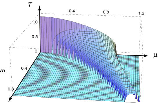
Figure 5: Phase structure of strong coupling 2-color QCD in the $\displaystyle T$-$\displaystyle\mu$-$\displaystyle m$ space. The surface represents the critical surface for the diquark condensation, which separates the region where $\displaystyle\Delta=0$ from the region where $\displaystyle\Delta\not=0$.

V SUMMARY AND CONCLUDING REMARKS

In this paper, we have studied the phase structure of 2-color QCD in the strong coupling limit formulated on the lattice. We have employed the $\displaystyle 1/d$ expansion (only in the spatial direction) and the mean field approximation to derive the free energy written in terms of the chiral condensate $\displaystyle\sigma$ and the diquark condensate $\displaystyle\Delta$ at finite $\displaystyle T$, $\displaystyle\mu$ and $\displaystyle m$. A major advantage of our approach is that we can derive rather simple formulae in an analytic way for the critical temperature ($\displaystyle T_{\mathrm{c}}$), the critical chemical potentials ($\displaystyle\mu_{\mathrm{c}}^{\mathrm{low}}$ and $\displaystyle\mu_{\mathrm{c}}^{\mathrm{up}}$), and the quark number density ($\displaystyle\rho$), which are useful to have physical insight into the problem. Although our results are in principle limited in the strong coupling, the behavior of $\displaystyle\sigma$, $\displaystyle\Delta$, and $\displaystyle\rho$ in the $\displaystyle T$-$\displaystyle\mu$-$\displaystyle m$ space has remarkable qualitative agreement with the recent lattice data. Since we do not have to rely on any assumption of small $\displaystyle\mu$ nor small $\displaystyle m$ in our approach, the strong coupling analysis presented in this paper is complementary to the results of the chiral perturbation theory and directly provides a useful guide to the lattice 2color-QCD simulations.

There are several directions worth to be explored starting from the present work. Among others, the derivation of an effective action written not only with the chiral and diquark fields but also with the Polyakov loop, $\displaystyle L(x)$, is interesting because this will allow us a full comparison for all the physical quantities calculated in our formalism and lattice simulations kog02 . This is a straightforward generalization of the works in fuku03 , which allows us to analyze $\displaystyle\langle L(x)\rangle$ under the influence of chiral and diquark condensates.

Also calculation of the meson and diquark spectra including pseudo-scalar and pseudo-diquark channels will give us deeper understanding about the non-static feature of the present system. Another direction is to study the response of the Bose liquid discussed in this paper under external fields. Although mesons and diquarks are color neutral in 2-color QCD, they can have electric charge so that the external electromagnetic field leads to a non-trivial change of the phase structure if the field intensity is enough strong. Generalization of the whole machinery in this paper to strong coupling 3-color QCD is also one of the challenging problems to be studied in the future.

Appendix A SUMMATION OVER THE MATSUBARA FREQUENCY

Let us first take the logarithm of Eq.(22);

$$\displaystyle\log\sqrt{\mathrm{Det}[G^{-1}]} \displaystyle=\sum_{m=1}^{N_{\tau}}\log\left[-\cos^{2}\left(k_{m}+\theta/N_{\tau}\right)+2Y\cos\left(k_{m}+\theta/N_{\tau}\right)+X^{2}\right]\,.$$ (46)

Here $\displaystyle X$ and $\displaystyle Y$ are defined as

$$\displaystyle X^{2}=\cosh^{2}\mu+M^{2}+\left(\frac{d}{2}\right)^{2}|\Delta|^{2}\,,\qquad Y=M\sinh\mu\,.$$ (47)

By differentiating $\displaystyle\log\sqrt{\mathrm{Det}[G^{-1}]}$ with respect to $\displaystyle X$, we obtain

$$\displaystyle\frac{\partial}{\partial X}\log\sqrt{\mathrm{Det}[G^{-1}]}=\frac{X}{\sqrt{X^{2}+Y^{2}}}\sum_{m=1}^{N_{\tau}}\left[\frac{1}{\cos\left(k_{m}+\theta/N_{\tau}\right)-Y+\sqrt{X^{2}+Y^{2}}}-\frac{1}{\cos\left(k_{m}+\theta/N_{\tau}\right)-Y-\sqrt{X^{2}+Y^{2}}}\right]\,.$$ (48)

Because $\displaystyle\cos(k_{m}+\theta/N_{\tau})$ is invariant under the shift $\displaystyle m\to m+N_{\tau}$, we can make the summation of $\displaystyle m$ over the range $\displaystyle m=-\infty$ to $\displaystyle m=+\infty$ with an appropriate degeneracy factor $\displaystyle\Omega$. Then the residue theorem enables us to replace the summation by a complex integral as

$$\displaystyle\begin{split}\frac{\partial}{\partial{X}}\log\sqrt{\mathrm{Det}[G^{-1}]}=\frac{X}{\sqrt{X^{2}+Y^{2}}}\frac{1}{\Omega}&\left[\oint\frac{\mathrm{d}z}{2\pi\mathrm{i}}\frac{1}{\cos\left(z+\theta/N_{\tau}\right)+k_{-}}\frac{-\mathrm{i}N_{\tau}}{1+\mathrm{e}^{\mathrm{i}N_{\tau}z}}-\sum_{\bar{z}}\frac{1}{-\sin\bar{z}}\frac{-\mathrm{i}N_{\tau}}{1+\mathrm{e}^{\mathrm{i}N_{\tau}\bar{z}}}\right.\\ &\left.-\oint\frac{\mathrm{d}w}{2\pi\mathrm{i}}\frac{1}{\cos\left(w+\theta/N_{\tau}\right)-k_{+}}\frac{-\mathrm{i}N_{\tau}}{1+\mathrm{e}^{\mathrm{i}N_{\tau}w}}+\sum_{\bar{w}}\frac{1}{-\sin\bar{w}}\frac{-\mathrm{i}N_{\tau}}{1+\mathrm{e}^{\mathrm{i}N_{\tau}\bar{w}}}\right]\,,\end{split}$$ (49)

where

$$\displaystyle k_{\pm}=\sqrt{X^{2}+Y^{2}}\pm Y\,.$$ (50)

Owing to the infinite range of the summation over $\displaystyle m$, we can choose the closed contour at infinity for the complex integrals with respect to $\displaystyle z$ and $\displaystyle w$, and thus such complex integrals go to zero. $\displaystyle\bar{z}$ and $\displaystyle\bar{w}$ are the residues satisfying

$$\displaystyle\cos\left(\bar{z}+\theta/N_{\tau}\right)+k_{-}=0\,,\qquad\cos\left(\bar{w}+\theta/N_{\tau}\right)-k_{+}=0\,.$$ (51)

Solving these equations, we obtain

$$\displaystyle\bar{z}+\theta/N_{\tau}=\pm\mathrm{i}E_{-}+\pi+2\pi n\,,\qquad\bar{w}+\theta/N_{\tau}=\pm\mathrm{i}E_{+}+2\pi n\,,\qquad\quad(n=-\infty,\dots,\infty)\,,$$ (52)

where

$$\displaystyle E_{\pm}=\mathrm{arccosh}k_{\pm}\,.$$ (53)

Substituting Eq. (52) into Eq. (49), we obtain

$$\displaystyle\frac{\partial}{\partial{X}}\log\sqrt{\mathrm{Det}[G^{-1}]}$$

$$\displaystyle=\frac{X}{\sqrt{X^{2}+Y^{2}}}\frac{1}{\Omega}\sum_{n=-\infty}^{\infty}\left[\frac{1}{-\mathrm{i}\sqrt{k_{-}^{2}-1}}\left(\frac{-\mathrm{i}N_{\tau}}{1+\mathrm{e}^{-N_{\tau}E_{-}-\mathrm{i}\theta+\mathrm{i}N_{\tau}\pi}}-\frac{-\mathrm{i}N_{\tau}}{1+\mathrm{e}^{N_{\tau}E_{-}-\mathrm{i}\theta+\mathrm{i}N_{\tau}\pi}}\right)\right.$$

$$\displaystyle\qquad\qquad\qquad\qquad\qquad\qquad\qquad\left.-\frac{1}{\mathrm{i}\sqrt{k_{+}^{2}-1}}\left(\frac{-\mathrm{i}N_{\tau}}{1+\mathrm{e}^{-N_{\tau}E_{+}-\mathrm{i}\theta}}-\frac{-\mathrm{i}N_{\tau}}{1+\mathrm{e}^{N_{\tau}E_{+}-\mathrm{i}\theta}}\right)\right]$$

$$\displaystyle=\frac{\partial E_{-}}{\partial X}\left\{\frac{N_{\tau}}{1+\mathrm{e}^{-N_{\tau}E_{-}-\mathrm{i}\theta}}-\frac{N_{\tau}}{1+\mathrm{e}^{N_{\tau}E_{-}-\mathrm{i}\theta}}\right\}+\frac{\partial E_{+}}{\partial X}\left\{\frac{N_{\tau}}{1+\mathrm{e}^{-N_{\tau}E_{+}-\mathrm{i}\theta}}-\frac{N_{\tau}}{1+\mathrm{e}^{N_{\tau}E_{+}-\mathrm{i}\theta}}\right\}$$

$$\displaystyle=\frac{\partial}{\partial X}\left[\log\left\{\mathrm{e}^{N_{\tau}E_{-}}+\mathrm{e}^{-\mathrm{i}\theta}\right\}+\log\left\{\mathrm{e}^{-N_{\tau}E_{-}}+\mathrm{e}^{-\mathrm{i}\theta}\right\}+\log\left\{\mathrm{e}^{N_{\tau}E_{+}}+\mathrm{e}^{-\mathrm{i}\theta}\right\}+\log\left\{\mathrm{e}^{-N_{\tau}E_{+}}+\mathrm{e}^{-\mathrm{i}\theta}\right\}\right]$$

$$\displaystyle=\frac{\partial}{\partial X}\left[-2\mathrm{i}\theta+2\log 2+\log\left\{\cos\theta+\cosh N_{\tau}E_{-}\right\}+\log\left\{\cos\theta+\cosh N_{\tau}E_{+}\right\}\right]\,.$$ (54)

We note that the degeneracy factor $\displaystyle\Omega$ is just canceled by the infinite degeneracy of the summation on $\displaystyle n$. Also we have used the fact that $\displaystyle N_{\tau}$ must be an even integer for the staggered fermion. After the integration with respect to $\displaystyle X$, we find that $\displaystyle\sqrt{\mathrm{Det}[G^{-1}]}$ is expressed in a rather simple form up to irrelevant factors,

$$\displaystyle\sqrt{\mathrm{Det}\left[G^{-1}_{ab}(m,n;\theta)\right]}=\left(\cos\theta+\cosh N_{\tau}E_{-}\right)\cdot\left(\cos\theta+\cosh N_{\tau}E_{+}\right)\,.$$ (55)

This is the final form shown in Eq. (23) in the text.

Appendix B PROOF OF $\displaystyle\sigma=0$ AT THE GLOBAL MINIMUM OF $\displaystyle F_{\mathrm{eff}}[\sigma,\Delta]|_{m=0}$

For $\displaystyle m=0$, it is useful to rewrite the free energy Eq. (27) in terms of the radial and angle variables,

$$\displaystyle\sigma=\lambda\sin\phi\,,\qquad|\Delta|=\lambda\cos\phi\,.$$ (56)

Then the free energy is

$$\displaystyle F_{\mathrm{eff}}[\lambda,\phi]=\frac{d}{2}\lambda^{2}-T\log\left\{1+4\cosh\left(E_{+}/T\right)\cdot\cosh\left(E_{-}/T\right)\right\}\,,$$ (57)

with the quasi-quark energy given by

$$\displaystyle E_{\pm}=\mathrm{arccosh}\left(\sqrt{(d/2)^{2}\lambda^{2}+\cosh^{2}\mu+(d/2)^{2}\lambda^{2}\sinh^{2}\mu\sin^{2}\phi}\pm\frac{d}{2}\lambda\sinh\mu\sin\phi\right)\,.$$ (58)

What we are going to prove here is that $\displaystyle F_{\mathrm{eff}}[\lambda,\phi]$ has the global minimum at $\displaystyle\phi=0$ for arbitrary $\displaystyle T$, $\displaystyle\mu$, and $\displaystyle\lambda$. Actually we can prove the following statement in a more abstract expression;

$$\displaystyle\cosh\{a\,\mathrm{arccosh}(b\,\mathrm{e}^{c})\}\cdot\cosh\{a\,\mathrm{arccosh}(b\,\mathrm{e}^{-c})\}\text{\, has the global maximum at $\displaystyle c=0$}\,,$$

$$\displaystyle\text{where }a>1,\text{ }b>1,\text{ and }-\log b<c<\log b\,.$$

We can apply this corollary to our problem to prove that $\displaystyle\phi=0$ is the global minimum of the free energy. Obviously $\displaystyle\phi=0$ turns out to be the global maximum of $\displaystyle\cosh(E_{+}/T)\cdot\cosh(E_{-}/T)$ once we substitute,

$$\displaystyle a=1/T,\quad b=\sqrt{(d/2)^{2}\lambda^{2}+\cosh^{2}\mu},\quad c=\log\left[\sqrt{1+(d\lambda/2b)^{2}\sinh^{2}\mu\sin^{2}\phi}+(d\lambda/2b)\sinh\mu\sin\phi\right]\,.$$ (59)

Thus we have proven that $\displaystyle F_{\mathrm{eff}}[\lambda,\phi]$ is globally minimized at $\displaystyle\phi=0$, in other words, the chiral condensate vanishes in the chiral limit.

References

-
(1)
R. Tamagaki, Prog. Theor. Phys. 44, 905 (1970).
M. Hoffberg, et al., Phys. Rev. Lett. 24, 775 (1970).
For further references, see the review:
T. Kunihiro, T. Muto, T. Takatsuka, R. Tamagaki, and T. Tatsumi, Prog. Theor. Phys. Suppl. 112, 1 (1993). -
(2)
A.B. Migdal, Nucl. Phys. A210, 421 (1972).
R.F. Sawyer and D.J. Scalapino, Phys. Rev. D 7, 953 (1973).
For further references, see the review in TAMA70 . -
(3)
D.B. Kaplan and A.E. Nelson,
Phys. Lett. B 175, 57 (1986).
For further references, see the review: C.H. Lee, Phys. Rept. 275, 255 (1996). -
(4)
J.C. Collins and M.J. Perry,
Phys. Rev. Lett. 34, 1353 (1975).
G. Baym and S.A. Chin, Phys. Lett. B 62, 241 (1976).
For further references, see the review:
H. Heiselberg and M. Hjorth-Jensen, Phys. Rept. 328, 237 (2000). -
(5)
N. Itoh, Prog. Theor. Phys. 44, 291 (1970).
A.R. Bodmer, Phys. Rev. D 4, 1601 (1971).
E. Witten, Phys. Rev. D 30, 272 (1984).
For further references, see the review:
J. Madsen, e-print: astro-ph/9809032. -
(6)
D. Bailin and A. Love, Phys. Rept. 107, 325 (1984).
M. Iwasaki and T. Iwado, Phys. Lett. B 350, 163 (1995).
R. Rapp, T. Schäfer, E.V. Shuryak, and M. Velkovsky, Phys. Rev. Lett. 81, 53 (1998).
M.G. Alford, K. Rajagopal, and F. Wilczek, Phys. Lett. B 422, 247 (1998).
For further references, see the reviews:
M.G. Alford, Ann. Rev. Nucl. Part. Sci. 51, 131 (2001).
K. Rajagopal and F. Wilczek, in At the Frontier of Particle Physics : Handbook of QCD, ed. M. Shifman (World Scientific Singapore, 2001), e-print: hep-ph/0011333. -
(7)
T. Tatsumi, Phys. Lett. B 489, 280 (2000).
A. Iwazaki and O. Morimatsu, Phys. Lett. B 571, 61 (2003). - (8) A. Nakamura, Phys. Lett. B 149, 391 (1984).
-
(9)
H. Abuki, T. Hatsuda, and K. Itakura,
Phys. Rev. D 65, 074014 (2002).
K. Itakura, Nucl. Phys. A715, 859 (2003). - (10) E. Dagotto, F. Karsch, and A. Moreo, Phys. Lett. B 169, 421 (1986).
- (11) E. Dagotto, A. Moreo, and U. Wolff, Phys. Lett. B 186, 395 (1987).
- (12) J.U. Klatke and K.H. Mutter, Nucl. Phys. B342, 764 (1990).
-
(13)
S. Hands, J.B. Kogut, M. Lombardo, and S.E. Morrison,
Nucl. Phys. B558, 327 (1999).
S. Hands, I. Montvay, S. Morrison, M. Oevers, L. Scorzato, and J. Skullerud, Eur. Phys. J. C 17, 285 (2000). - (14) J.B. Kogut, D. Toublan, and D.K. Sinclair, Phys. Lett. B 514, 77 (2001); Nucl. Phys. B642, 181 (2002); Phys. Rev. D 68, 054507 (2003).
- (15) S. Muroya, A. Nakamura, and C. Nonaka, Phys. Lett. B 551, 305 (2003).
- (16) G.W. Carter and D. Diakonov, Phys. Rev. D 60, 016004 (1999).
- (17) B. Vanderheyden and A.D. Jackson, Phys. Rev. D 64, 074016 (2001).
-
(18)
J.B. Kogut, M.A. Stephanov, and D. Toublan,
Phys. Lett. B 464, 183 (1999).
J.B. Kogut, M.A. Stephanov, D. Toublan, J.J.M. Verbaarschot, and A. Zhitnitsky, Nucl. Phys. B582, 477 (2000). - (19) K. Splittorff, D. Toublan, and J.J.M. Verbaarschot, Nucl. Phys. B639, 524 (2002).
- (20) J. Wirstam, J.T. Lenaghan, and K. Splittorff, Phys. Rev. D 67, 034021 (2003).
- (21) P. Hasenfratz and F. Karsch, Phys. Lett. B 125, 308 (1983).
-
(22)
H. Kluberg-Stern, A. Morel, and B. Petersson,
Nucl. Phys. B215 [FS7], 527 (1983).
H. Kluberg-Stern, A. Morel, O. Napoly, and B. Petersson, Nucl. Phys. B220 [FS8], 447 (1983). -
(23)
W. Pauli, Nuovo Cimento 6, 205 (1957).
F. Gürsey, Nuovo Cimento 7, 411 (1958).
A. Smilga and J.J.M. Verbaarshot, Phys. Rev. D 51, 829 (1995). -
(24)
This integral is known as the pfaffian. See e.g.,
J. Zinn-Justin, Quantum Field Theory and Critical Phenomena (Clarendon Press, Oxford, 1989), Chapter 1. - (25) T. Hatsuda, Nucl. Phys. A492, 187 (1989).
- (26) K. Fukushima, Phys. Lett. B 553, 38 (2003); Phys. Rev. D 68, 045004 (2003).