1cm DESY 03-069 June 05, 2003

Motivated by the simplicity and direct phenomenological applicability of field-theoretic orbifold constructions in the context of grand unification, we set out to survey the immensely rich group-theoretical possibilities open to this type of model building. In particular, we show how every maximal-rank, regular subgroup of a simple Lie group can be obtained by orbifolding and determine under which conditions rank reduction is possible. We investigate how standard model matter can arise from the higher-dimensional SUSY gauge multiplet. New model building options arise if, giving up the global orbifold construction, generic conical singularities and generic gauge twists associated with these singularities are considered. Viewed from the purely field-theoretic perspective, such models, which one might call conifold GUTs, require only a very mild relaxation of the constraints of orbifold model building. Our most interesting concrete examples include the breaking of E₇ to SU(5) and of E₈ to SU(4)$\times$SU(2)$\times$SU(2) (with extra factor groups), where three generations of standard model matter come from the gauge sector and the families are interrelated either by SU(3) R-symmetry or by an SU(3) flavour subgroup of the original gauge group.

1 Introduction

Arguably, the way in which fermion quantum numbers are explained by $\mathrm{SU}(5)$-related grand unified theories (GUTs) represents one of the most profound hints at fundamental physics beyond the standard model (SM) [1, 2] (also [3]). In this context supersymmetry (SUSY), usually invoked to solve the hierarchy problem and to achieve gauge coupling unification, receives a further and maybe even more fundamental motivation: If the underlying gauge group contains gauge bosons with the quantum numbers of SM matter, SUSY enforces the existence of the corresponding fermions. This is very naturally realized in a higher-dimensional setting, where the extra-dimensional gauge field components and their fermionic partners can be light even though the gauge group is broken at a high scale (see, e.g., [5, 4, 7, 6]).

Thus, we adopt the point of view that, at very high energies, we are faced with a super Yang-Mills (SYM) theory in $d>4$ dimensions which is compactified in such a way that the resulting 4d effective theory has smaller gauge symmetry (ideally that of the SM) and contains the light SM matter and Higgs fields. In the simplest models the compactification space is flat except for a finite number of singularities. Although this situation arises naturally in heterotic string theory [8, 9] and has thus been extensively studied in string model building, it has only recently been widely recognized that many interesting phenomenological implications do not depend on the underlying quantum gravity model and can be studied directly in higher-dimensional field theory [10] (also [11, 12, 13, 14, 15]).

In the purely field-theoretic context, one has an enormous freedom in choosing the underlying gauge group, the number of extra dimensions and their geometry, the way in which the compactification reduces the gauge symmetry (e.g., the type of orbifold breaking), the possible extra field content and couplings in the bulk and at the singularities. Although, using all this freedom, realistic models can easily be constructed, there is so far no model which, by its simplicity and direct relation to the observed field content and couplings, appears to be as convincing as, say, the generic SU(5) unification idea. However, we feel that the search for such a model in the framework of higher-dimensional SYM theory is promising and that a thorough understanding of the group-theoretical possibilities of orbifold-breaking (without the restrictions of string theory) will be valuable in this context. The present paper is aimed at the exploration of these possibilities and their application to orbifold GUT model building. In particular, we are interested in methods for breaking larger gauge groups to the SM, in possibilities for rank reduction, and in the derivation of matter fields from the adjoint representation.

In Sec. 2, we collect some of the most relevant facts and methods of group theory, which serves in particular to fix our notation and conventions for the rest of the paper.

In Sec. 3, we begin by recalling the generic features of field theoretic orbifold models. It is then shown how orbifolding can break a simple Lie group to any of its maximal regular subgroups. This implies, in particular, that any regular subgroup (possibly times extra simple groups and U(1) factors) can be obtained by orbifold-breaking and opens up an enormous variety of model building possibilities.

We continue in Sec. 4 by exploring rank reduction by non-Abelian orbifolding. We show that simple group factors can always be broken completely. In cases where a maximal subgroup contains an extra U(1) factor, this factor can only be broken under certain conditions. We give a criterion specifying when the extra U(1) cannot be removed. As an interesting observation, we note that under special circumstances rank reduction based on inner automorphisms is also possible on Abelian orbifolds.

In Sec. 5, we discuss manifolds with conical singularities which can not be obtained by orbifolding. In particular, such ‘conifolds’ can have conical singularities with arbitrary deficit angle. In addition, we consider the possibility of having Wilson lines with unrestricted values wrapped around the singularities of orbifolds or conifolds. All this gives rise to many new possibilities for gauge symmetry breaking and for the generation of three families of chiral matter from the field content of the SYM theory.

Finally, Sec. 6 discusses three specific models, one with E₇ broken to SU(5) and two with E₈ broken to SU(4)$\times$SU(2)$\times$SU(2) (with extra factor groups). In all cases, three generations of SM matter come from the gauge sector. In one of the E₈ models, the families are interrelated by an SU(3) R-symmetry, while in the two other models an SU(3) flavour subgroup of the original gauge group appears.

Sec. 7 contains our conclusions and outlines future perspectives and open questions.

2 Basics of group theory

This section is not meant as an introduction to group theory, but merely serves to remind the reader of some crucial facts and to fix our notation. Relevant references include the classic papers of Dynkin [16, 17, 18] (partially collected in [19]), various textbooks (e.g., [20, 22, 21]), and the review article [23].

For each finite-dimensional, complex Lie algebra $\mathfrak{g}$, the maximal Abelian subalgebra $\mathfrak{h}$, which is unique up to automorphisms, is called Cartan subalgebra. Its dimension defines the rank $r$ of the Lie algebra and its generators will be denoted by $\{\boldsymbol{H}_{i}\}_{i=1}^{r}$. They are orthonormal with respect to the Killing metric, i.e., they fulfill the relation

$$\operatorname{tr}(\boldsymbol{H}_{i}\,\boldsymbol{H}_{j})\,=\,\lambda\,\delta_{ij}\;,$$ (2.1)

where the trace is taken in the adjoint representation and $\lambda$ is some constant.

The remaining generators can be chosen such that

$$[\boldsymbol{H}_{i},\boldsymbol{E}_{\alpha}]\,=\,\alpha_{i}\,\boldsymbol{E}_{\alpha}\;,$$ (2.2)

and are called roots. They are normalized as in Eq. (2.1). Each root $\boldsymbol{E}_{\alpha}$ is determined uniquely by the root vector $\alpha$, which is an element of an $r$-dimensional Euclidean space, called the root space. The set of all roots will be denoted by $\Sigma$. The $\boldsymbol{E}_{\alpha}$ obey the commutation relations

$$\left[\boldsymbol{E}_{\alpha},\boldsymbol{E}_{\beta}\right]\,=\,N_{\alpha,\beta}\,\boldsymbol{E}_{\alpha+\beta}\;,$$ (2.3)

where the $N_{\alpha,\beta}$ are normalization constants, and $N_{\alpha,\beta}=0$ means that $\alpha+\beta\not\in\Sigma$.

We introduce an order in the root space by

$$\alpha-\beta>0\quad:\Leftrightarrow\quad\text{first non-vanishing component of}\>\alpha-\beta>0\;.$$ (2.4)

Correspondingly, we will call a root ‘positive’ if the first non-vanishing component in the root basis is positive. The smallest $r$ positive roots are called simple and will be denoted by $\{\alpha_{(i)}{}\}_{i=1}^{r}$. They are linearly independent, and any root can be expressed by a linear combination

$$\alpha=\sum\limits_{i=1}^{r}k^{i}\,\alpha_{(i)}{}$$ (2.5)

with integer coefficients $k^{i}$. Motivated by this, a basis

$$e_{(i)}\,=\,\frac{2}{|\alpha_{(i)}|^{2}}\alpha_{(i)}{}\;,$$ (2.6)

is introduced. The normalization factor will be justified later.

In this basis, the Euclidean metric of the root space is characterized by $g_{ij}=e_{(i)}\cdot e_{(j)}$. It is useful to consider also the vector space dual to the root space which, given the existence of a metric in the root space, can be identified with the root space by the canonical isomorphism. It is spanned by the so-called fundamental weights $\mu^{(i)}$ ($1\leq i\leq r$) which are defined by

$$\mu^{(i)}\cdot e_{(j)}\,=\,\delta^{i}_{j}\;.$$ (2.7)

The components with respect to the $\mu^{(i)}$ basis are called Dynkin labels. Correspondingly, the $\mu^{(i)}$ are frequently referred to as the Dynkin basis, in which case the $e_{(i)}$ are called the dual basis. The constant $\lambda$ in Eq. (2.1) is chosen such that $|\alpha_{(i)}{}|^{2}=2$ for the longest of the simple roots. Then the normalization factor in Eq. (2.6) ensures that the Dynkin label of any weight (weights being the analogues of the vectors $\alpha$ in an arbitrary representation) is integer valued.

The Dynkin labels of each simple root are given by the corresponding row of the Cartan-matrix

$$A_{ij}\,=\,2\,\frac{\alpha_{(i)}{}\cdot\alpha_{(j)}{}}{|\alpha_{(j)}{}|^{2}}\,=\,g_{ij}\,\frac{|\alpha_{(i)}{}|^{2}}{2}\;,$$ (2.8)

which encodes the metric of the root space.

It is well-known that there exist four infinite series of simple groups $\mathrm{A}_{r}$, $\mathrm{B}_{r}$, $\mathrm{C}_{r}$ and $\mathrm{D}_{r}$, corresponding to the classical groups, and the exceptional groups $\mathrm{G}_{2}$, $\mathrm{F}_{4}$, $\mathrm{E}_{6}$, $\mathrm{E}_{7}$ and $\mathrm{E}_{8}$. The scalar products of the simple roots determine the Dynkin diagrams (cf. the captions of Tab. 2.1 and Tab. 2.2).

For later convenience, we introduce the most negative root $\theta$, which leads us to the extended Dynkin diagrams as listed in Tab. 2.1 and in Tab. 2.2.

Name	Real algebra	Extended Dynkin diagram
$\mathrm{A}_{n}$	$\mathfrak{su}(n+1)$
$\mathrm{B}_{n}$	$\mathfrak{so}(2n+1)$
$\mathrm{C}_{n}$	$\mathfrak{sp}(2n)$
$\mathrm{D}_{n}$	$\mathfrak{so}(2n)$

Table 2.1: The classical Lie algebras and the corresponding extended Dynkin diagrams. The shorter roots are hatched. If the simple roots $\alpha_{(i)}{}$ and $\alpha_{(j)}{}$ enclose an angle of $90^{\circ}$, $120^{\circ}$ or $135^{\circ}$, they are connected by 0, 1 or 2 lines, respectively.

Name	Extended Dynkin diagram
$\mathrm{G}_{2}$
$\mathrm{F}_{4}$
$\mathrm{E}_{6}$
$\mathrm{E}_{7}$
$\mathrm{E}_{8}$

Table 2.2: The five exceptional Lie algebras. In $\mathrm{G}_{2}$, the two simple roots enclose $150^{\circ}$, which is indicated by a triple line.

3 Obtaining all regular subgroups by orbifolding

Orbifold GUTs [10, 11, 12, 13, 14, 15] are based on a gauge theory on $\mathbbm{R}^{4}\times M$, where $M$ is a manifold with some discrete symmetry group $K$. In addition to the action of $K$ on $M$, an action in internal space can be chosen using a homomorphism from $K$ to the automorphism group of the Lie algebra of the gauge theory. If the classical field space is restricted by the requirement of $K$ invariance, a gauge theory on a manifold with singularities, $M/K$, results in general. We assume that $M/K$, though not necessarily $M$, is compact. At the singularities, which correspond to the fixed points of the space-time action of $K$, the gauge symmetry may be restricted (orbifold breaking). An early review of the structure of such models is contained in [24] (for more recent reviews see, e.g., [25, 26]).

One of the main features of orbifold GUTs is the possibility of breaking a gauge group without the use of Higgs fields. The orbifold field theory possesses the full (unified) gauge symmetry everywhere except for certain fixed points. Although this fixed-point breaking is ‘hard’, in the sense that the action does not possess the full gauge symmetry, gauge coupling unification is not lost due to the numerical dominance of the bulk. Furthermore, it is attractive for model building purposes that the symmetry – and hence the field content – is characterized by different groups at different geometric locations, such as the various fixed points and the bulk.

In this paper, we focus on inner-automorphism breaking, i.e., a homomorphism from $K$ to the gauge group $G$ together with the adjoint action of $G$ on itself is used to define the transformation of gauge fields under $K$. Only gauge fields invariant under $K$ have zero modes. The corresponding generators define the symmetry of the low-energy effective theory, which is a subgroup of $G$. We will assume that $G$ is simple since it is straightforward to extend our analysis to the product of simple groups and $\mathrm{U}(1)$ factors.

To discuss the breaking in more detail, consider a group element $P$ which is the image of some element of $K$. Any $P\in G$ can be written as an exponential of some Lie algebra element and is therefore contained in some U(1) subgroup of $G$. Constructing a maximal torus starting from this U(1) and using the fact that the maximal torus in a compact Lie group is unique up to isomorphism [27], it becomes clear that one can always write

$$P\,=\,\exp(-2\pi\mathrm{i}\,V\cdot\boldsymbol{H})\;,$$ (3.1)

with some real vector $V$. Hence, the action of the gauge twist on the Lie algebra is given by

$$P\,\boldsymbol{E}_{\alpha}\,P^{-1} = \exp(-2\pi\mathrm{i}\,\alpha\cdot V)\,\boldsymbol{E}_{\alpha}\;,$$ (3.2a)

$$P\,\boldsymbol{H}_{i}\,P^{-1} = \boldsymbol{H}_{i}\;.$$ (3.2b)

We can also choose to write $P=\exp(-2\pi\mathrm{i}\,\xi\,\boldsymbol{T})$, where $\boldsymbol{T}$ is a normalized Lie algebra element, $\xi\in\mathbbm{R}$, and $\xi\,\boldsymbol{T}=V\cdot\boldsymbol{H}$. For generic $\xi$, $P$ commutes with precisely those Lie algebra elements with which $\boldsymbol{T}$ commutes. Thus, the breaking is the same as would follow from a Higgs VEV in the adjoint representation.

However, it is clear from Eq. (3.2a) that, for certain values of $\xi$, some of the $\boldsymbol{E}_{\alpha}$ may pick up phases which are an integer multiple of $2\pi$ and are thus left invariant. In this case, the surviving subgroup is larger than the one obtained from an adjoint VEV proportional to $\boldsymbol{T}$. This possibility is of particular interest since, in certain cases, such as the breaking of $\mathrm{SO}(10)$ to $\mathrm{SU}(4)\times\mathrm{SU}(2)\times\mathrm{SU}(2)$, the relevant subgroup can not be realized by using Higgs VEVs in the adjoint or any smaller representation.

3.1 Orbifold-breaking to any maximal regular subgroup

We now show that, given a simple group $G$ and a maximal regular subgroup $H$, there exists a $P\in G$ such that

$$H\,=\,\{g\in G;\;P\,g\,P^{-1}=g\}\,.$$ (3.3)

In other words, every maximal regular subgroup can be generated by an orbifold twist.

In order to prove this statement, we first recall Dynkin’s prescription for generating semi-simple subgroups. It starts with the Dynkin diagram, extends it by adding the most negative root, and then removes one of the simple roots, the resulting Dynkin diagram being that of a semi-simple subgroup. As demonstrated in [18] (cf. Theorem 5.3), any maximal-rank, semi-simple subgroup of a given group can be obtained by successive application of this prescription. Maximal subgroups can always be obtained in the first application.

To implement Dynkin’s prescription and remove the simple root $\alpha_{(i)}$, one can use the fundamental weight $\mu^{(i)}$ and choose

$$P\,=\,\exp\left(\frac{2\pi\mathrm{i}}{n}\,\frac{2}{|\alpha_{(i)}{}|^{2}}\,\mu^{(i)}\cdot\boldsymbol{H}\right)\;.$$ (3.4)

Obviously, $P$ commutes with all simple roots $\boldsymbol{E}_{\alpha_{(j)}}$ where $j\neq i$. To discuss the roots $\alpha_{(i)}$ and $\theta$, recall first that

$$\theta=-\sum_{k=1}^{r}c_{k}\,\alpha_{(k)}{}$$ (3.5)

with the $c_{k}$ being known as Coxeter labels. They can be read off from Tab. 3.1. Such group-theoretical methods were used in [29] in the context of E₈ breaking in string theory.

Group	Dynkin labels of $\Lambda_{\mathrm{ad}}$	Coxeter labels
$\mathrm{A}_{n}\simeq\mathrm{SU}(n+1)$	$(1,0,\dots 0,1)$	$(1,1,\dots 1)$
$\mathrm{B}_{n}\simeq\mathrm{SO}(2n+1)$	$(0,1,0,\dots)$	$(1,2,2,\dots 2,2)$
$\mathrm{C}_{n}\simeq\mathrm{Sp}(2n)$	$(2,0,0,\dots)$	$(2,2,\dots 2,1)$
$\mathrm{D}_{n}\simeq\mathrm{SO}(2n)$	$(0,1,0,\dots)$	$(1,2,2,\dots 2,1,1)$
$\mathrm{G}_{2}$	$(1,0)$	$(2,3)$
$\mathrm{F}_{4}$	$(1,0,0,0)$	$(2,3,4,2)$
$\mathrm{E}_{6}$	$(0,0,0,0,0,1)$	$(1,2,3,2,1,2)$
$\mathrm{E}_{7}$	$(1,0,0,0,0,0,0)$	$(2,3,4,3,2,1,2)$
$\mathrm{E}_{8}$	$(0,0,0,0,0,0,1,0)$	$(2,4,6,5,4,3,2,3)$

Table 3.1: Highest weights of the adjoint representations, denoted by $\Lambda_{\mathrm{ad}}$, of the simple groups in the Dynkin basis and their Coxeter labels.

Thus, we can write the orbifold action on the two roots $\boldsymbol{E}_{\alpha_{(i)}{}}$ and $\boldsymbol{E}_{\theta}$ as

$$P\,\boldsymbol{E}_{\alpha_{(i)}{}}\,P^{-1} = e^{2\pi\mathrm{i}/n}\,\boldsymbol{E}_{\alpha_{(i)}{}}\;,$$ (3.6a)

$$P\,\boldsymbol{E}_{\theta}\,P^{-1} = e^{-2\pi\mathrm{i}\,c_{i}/n}\,\boldsymbol{E}_{\theta}\;,$$ (3.6b)

which shows that, for $\boldsymbol{E}_{\theta}$ to be invariant and $\boldsymbol{E}_{\alpha_{(i)}{}}$ to be projected out, we need $c_{i}\neq 1$. Using Tab. 3.1 and the corresponding Dynkin diagrams, it is easy to convince oneself that $c_{i}=1$ occurs only for those $i$ where the Dynkin-prescription with removal of $\alpha_{(i)}$ returns the original diagram. Thus, all non-trivial subgroups accessible by the Dynkin-prescription can be obtained by $\mathbbm{Z}_{n}$ orbifolding with $n=c_{i}$.

An interesting and subtle observation can be made in those cases where $c_{i}$ is not prime (only $c_{i}=4$ and $c_{i}=6$ occur). If $c_{i}=n=m\cdot k$, a $\mathbbm{Z}_{m}$ twist generated by $P^{k}$ is sufficient to project out $\boldsymbol{E}_{\alpha_{(i)}{}}$ while keeping $\boldsymbol{E}_{\theta}$, yet the surviving subgroup is larger than for the corresponding $\mathbbm{Z}_{n}$ twist $P$ and its Dynkin diagram is not the one obtained by Dynkin’s prescription. These are the famous five cases where Dynkin’s prescription produces a subgroup that is not maximal [30]. They occur when removing the 3rd root of $\mathrm{F}_{4}$, the 3rd root of $\mathrm{E}_{7}$, and the 2nd, 3rd or 5th root of $\mathrm{E}_{8}$.

It is easy to see that for $c_{i}$ prime the produced subgroup is maximal. Indeed, the roots of $G$ which are not roots of the subgroup $H$ can be classified according to their ‘level’ relative to $\alpha_{(i)}$, i.e., according to the coefficient of $\alpha_{(i)}$ in their decomposition in terms of simple roots. If a subgroup $H^{\prime}$ with $H\subset H^{\prime}\subset G$ exists, one of the levels below $c_{i}$ (which is the highest level) and above 1 must be occupied (i.e., its roots belong to $H^{\prime}$). Let $\ell$ be the smallest of those levels. All multiples of $\ell$ are also occupied and, since $c_{i}$ is not a multiple, the difference between $c_{i}$ and one of those multiples must be smaller than $\ell$. However, by the way in which the commutation relations are realized in root space, the level corresponding to this difference must also be occupied. This is in contradiction to $\ell$ being the smallest occupied level in $H^{\prime}$.

Having dealt with all semi-simple maximal subgroups, we now come to maximal subgroups containing $\mathrm{U}(1)$ factors. Given a maximal subgroup $H$ with $\mathrm{U}(1)$ factor, i.e., $G\supset H\times\mathrm{U}(1)$, we can always break to a subgroup $H^{\prime}$ by an adjoint VEV along this $\mathrm{U}(1)$ direction or a corresponding orbifold twist. It is obvious that $H\subset H^{\prime}$ since, by the definition of $H$, all its elements commute with the generator of the above $\mathrm{U}(1)$. Thus, $H=H^{\prime}$ and our analysis of orbifold breaking to all maximal-rank regular subgroups is complete. The maximal regular subgroups and the corresponding twists are listed in Tab. A.1 in App. A. We would also like to mention that the maximal subgroups with $\mathrm{U}(1)$ factors can be obtained by removing one node of the original Dynkin diagram which carries Coxeter label 1, and adding the $\mathrm{U}(1)$ factor.

Now that it is clear how a given maximal regular subgroup can be generated by an orbifold twist, we can take the opposite point of view and ask to which subgroups an arbitrary given gauge twist $P=\exp{(-2\pi\mathrm{i}\,\xi\,\boldsymbol{T}})$ can lead. Since an adjoint VEV proportional to $\boldsymbol{T}$ breaks to a maximal rank subgroup $H\times$U(1), where the $\mathrm{U}(1)$ is generated by $\boldsymbol{T}$, we can classify all $\boldsymbol{T}$’s by such maximal subgroups. These are given in various tables (see, in particular, [23]) together with the branching rules for the adjoint representation

$$\operatorname{ad}G\,\to\,\operatorname{ad}H\oplus\boldsymbol{1}(0)\oplus\boldsymbol{R}_{1}(q_{1})\oplus\boldsymbol{R}_{2}(q_{2})\oplus\dots\;.$$ (3.7)

Here the $\boldsymbol{R}_{i}$ are representations under $H$ and $q_{i}$ the corresponding $\mathrm{U}(1)$ charges. Under the gauge twist, the $\boldsymbol{R}_{i}$ transform as $\boldsymbol{R}_{i}\to e^{2\pi\mathrm{i}\,\xi q_{i}}\,\boldsymbol{R}_{i}$. This allows us to determine which particular sets of generators $\boldsymbol{R}_{i}$ survive for specific values of $\xi$, i.e., to identify those $\boldsymbol{R}_{i}$ for which $\xi q_{i}=0\mod\mathbbm{Z}$. Together with the generators of $H\times$U(1), they form the Lie algebra of the new surviving subgroup $H^{\prime}\supset H\times$U(1). Thus, by analyzing all subgroups $H\times$U(1) and all values of $\xi$, our classification is complete.

Finally, we would like to comment on the minimal order of the twist required to achieve the breaking $G\to H$. A very useful approximate rule is that under a $\mathbbm{Z}_{n}$ twist

$$\dim H\,\gtrsim\,r+\frac{\dim G-r}{n}\;.$$ (3.8)

The reason is that the $r$ Cartan generators survive the twist anyway, and the phases of the roots are proportional to a level relative to a simple root $\alpha_{(i)}{}$, or linear combination of such levels. Due to the symmetries of the root lattice, the phases are therefore almost evenly distributed among $\{0,2\pi/n,4\pi/n,\dots(n-1)2\pi/n\}$ where an excess at 0 is possible if the twist acts trivially on a certain part of the algebra. An inspection of Tab. A.1 confirms our rule which becomes the more accurate the larger the group is.

3.2 Some examples from the series $\boldsymbol{\mathrm{SO}(10)\subset\mathrm{E}_{6}\subset\mathrm{E}_{7}\subset\mathrm{E}_{8}}$

At this point, some examples are in order. Let us start with the $\mathrm{SO}(10)$ GUT which contains the Georgi-Glashow group $G_{\mathrm{GG}}=\mathrm{SU}(5)\otimes\mathrm{U}(1)$ and the Pati-Salam group $G_{\mathrm{PS}}=\mathrm{SU}(4)\times\mathrm{SU}(2)\times\mathrm{SU}(2)$ as subgroups. These properties are nicely illustrated by using Dynkin’s prescription:

(a) Extended Dynkin diagram of $\mathrm{SO}(10)$.

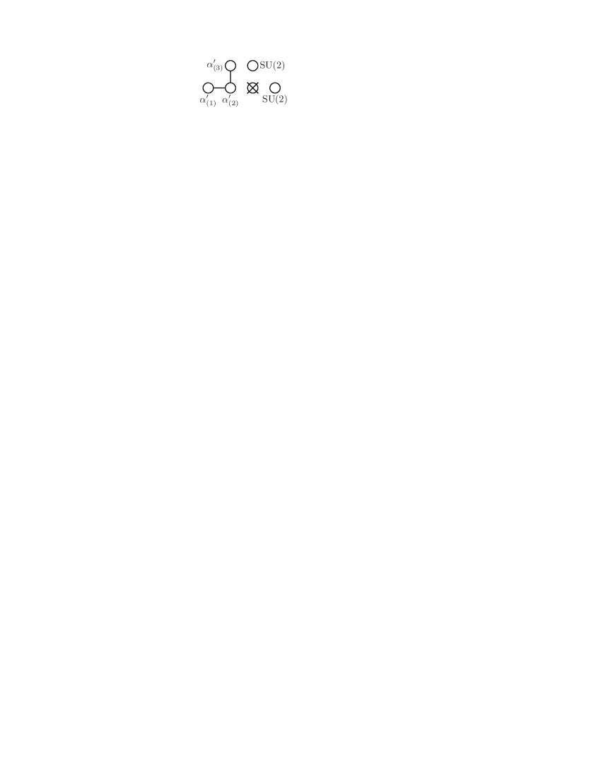
(b) Breaking to $G_{\mathrm{PS}}$.

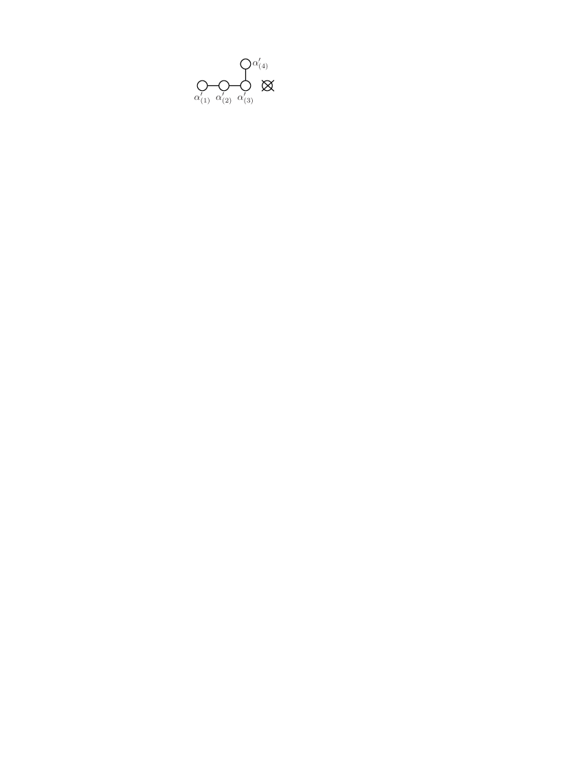
(c) Breaking to $G_{\mathrm{GG}}$.

Figure 1: The breaking to the Pati-Salam and Georgi-Glashow subgroups of $\mathrm{SO}(10)$ can be illustrated by removing the $\alpha_{(3)}{}$ (or $\alpha_{(2)}{}$) node of the extended Dynkin diagram (a) as shown in (b) or by removing $\alpha_{(5)}{}$ (or $\alpha_{(4)}{}$) as shown in (c).

Starting from the extended Dynkin diagram (cf. Fig. 1), the diagram of $\mathrm{G}_{\mathrm{PS}}$ is obtained by deleting the third (or second) node. Deleting the fourth (or fifth) node of the original diagram, we arrive at $G_{\mathrm{GG}}$. According to Sec. 3.1, twists which break to $G_{\mathrm{GG}}$ and $\mathrm{G}_{\mathrm{PS}}$, respectively, can be written as

$$P_{\mathrm{PS}} = \exp(\pi\mathrm{i}\,\mu^{(3)}\cdot\boldsymbol{H})\;,$$ (3.9a)

$$P_{\mathrm{GG}} = \exp(\pi\mathrm{i}\,\mu^{(4)}\cdot\boldsymbol{H})\;,$$ (3.9b)

where we exploited the fact that $|\alpha_{(i)}{}|^{2}=2$ in simply-laced groups.

In [14, 15], it was shown that by identifying these two twists as generators of $\mathbbm{Z}_{2}\times\mathbbm{Z}_{2}^{\prime}$, the gauge symmetry on a $\mathbbm{T}^{2}/(\mathbbm{Z}_{2}\times\mathbbm{Z}_{2}^{\prime})$ orbifold is reduced to $G_{\mathrm{SM}}^{\prime}=\mathrm{SU}(3)\times\mathrm{SU}(2)\times\mathrm{U}(1)_{\mathrm{Y}}\times\mathrm{U}(1)_{\chi}\subset\mathrm{SO}(10)$. The resulting geometry can be visualized as a ‘pillow’ with the corners corresponding to the fixed points.

The relevant group theory can be understood as follows: $\mu^{(3)}\cdot\boldsymbol{H}$ and $\mu^{(4)}\cdot\boldsymbol{H}$ are the $\mathrm{U}(1)$ generators appearing in $G_{\mathrm{SM}}^{\prime}$. The corresponding decomposition of the adjoint representation of $\mathrm{SO}(10)$ reads

$$\boldsymbol{45} \to (\boldsymbol{1},\boldsymbol{1})_{(6,4)}\oplus(\overline{\boldsymbol{3}},\boldsymbol{1})_{(-4,4)}\oplus(\boldsymbol{3},\boldsymbol{2})_{(1,4)}\oplus(\boldsymbol{3},\boldsymbol{2})_{(-5,0)}$$ (3.10)

$${}\oplus(\boldsymbol{1},\boldsymbol{1})_{(-6,-4)}\oplus(\boldsymbol{3},\boldsymbol{1})_{(4,-4)}\oplus(\overline{\boldsymbol{3}},\boldsymbol{2})_{(-1,-4)}\oplus(\overline{\boldsymbol{3}},\boldsymbol{2})_{(5,0)}$$

$${}\oplus(\boldsymbol{8},\boldsymbol{1})_{(0,0)}\oplus(\boldsymbol{1},\boldsymbol{3})_{(0,0)}\oplus(\boldsymbol{1},\boldsymbol{1})_{(0,0)}\oplus(\boldsymbol{1},\boldsymbol{1})_{(0,0)}\;,$$

where the $\mathrm{SU}(3)\times\mathrm{SU}(2)$ representations are given in boldface and the U(1) charges $(q_{Y},q_{\chi})$ appear as index. The twist which is responsible for this breaking is generated by a linear combination of the generators of the two $\mathrm{U}(1)$s, and rotates the charged representations by a phase $2\pi\,(y\,q_{Y}+\chi\,q_{\chi})$. For some combinations of $\chi$ and $y$, the orbifold breaking preserves a larger symmetry than adjoint breaking. For example, if $(\boldsymbol{1},\boldsymbol{1})_{(6,4)}$, $(\boldsymbol{1},\boldsymbol{1})_{(-6,-4)}$, $(\overline{\boldsymbol{3}},\boldsymbol{1})_{(-4,4)}$ and $(\boldsymbol{3},\boldsymbol{1})_{(4,-4)}$ survive (e.g., by taking $\chi=0$ and $y=1/2$), the resulting gauge group is $G_{\mathrm{PS}}$. If, on the other hand, $(\boldsymbol{3},\boldsymbol{2})_{(-5,0)}$ and $(\overline{\boldsymbol{3}},\boldsymbol{2})_{(5,0)}$ survive (e.g., by taking $\chi=1/8$ and $y=0$), the resulting gauge group is $G_{\mathrm{GG}}$. It is then clear that $G_{\mathrm{SM}}^{\prime}$ results as an intersection of gauge fields surviving $P_{\mathrm{PS}}$ and $P_{\mathrm{GG}}$. The breaking to $G_{\mathrm{SM}}^{\prime}$ can also be realized on a single $\mathbbm{Z}_{4}$ fixed point, e.g., by using $\chi=1/16$ and $y=1/4$.

As a side-remark, let us restate the above discussion in terms of matrices: Consider the adjoint VEV

$$v\,=\,\operatorname{diag}(a,a,a,b,b)\otimes\left(\begin{array}[]{cc}0&1\\ -1&0\end{array}\right)\;,$$ (3.11)

which breaks $\mathrm{SO}(10)$ to $G_{\mathrm{SM}}^{\prime}$ [22]. For the special case $a=\pm b$, the remaining symmetry is larger and equal to $G_{\mathrm{GG}}$. Alternatively, these breakings can be realized by a gauge twist $P=\exp[2\pi\mathrm{i}\,v]$ at an orbifold fixed point. In this case, taking $a=0$ and $b=1/2$ yields $P_{\mathrm{PS}}$ and $a=b=1/4$ yields $P_{\mathrm{GG}}$.

Let us now turn to the task of extending the ‘pillow’ of Asaka, Buchmüller and Covi [31] along the chain of exceptional groups $\mathrm{SO}(10)\subset\mathrm{E}_{6}\subset\mathrm{E}_{7}\subset\mathrm{E}_{8}$. A related discussion has already appeared in [32]. However, as will become clear below, we disagree with some of the results of that paper.

The obvious generalizations of (3.9) for the exceptional groups read

$$P_{\mathrm{GG}}^{(r)} := \exp(\pi\mathrm{i}\,\mu^{(r-1)}\cdot\boldsymbol{H})\;,$$ (3.12a)

$$P_{\mathrm{PS}}^{(r)} := \exp(\pi\mathrm{i}\,\mu^{(r-2)}\cdot\boldsymbol{H})\;.$$ (3.12b)

In other words, the generalizations of $P_{\mathrm{GG}}$ and $P_{\mathrm{PS}}$ to higher groups along the above chain remove the nodes $\alpha_{(r-1)}{}$ and $\alpha_{(r-2)}{}$ respectively. This is illustrated in Tab. 3.2.

$$\begin{array}[]{|l|l|}\hline\cr\vbox{\hbox{\includegraphics{DynkinD5toGGPS.eps}}}&\begin{array}[]{l}\begin{array}[]{rcl}\mathrm{SO}(10)&\xrightarrow{P_{\mathrm{GG}}\phantom{\big{|}}}&\mathrm{SU}(5)\times\mathrm{U}(1)\\ \mathrm{SO}(10)&\xrightarrow{P_{\mathrm{PS}}}&\mathrm{SU}(4)\times\mathrm{SU}(2)\times\mathrm{SU}(2)\\ \mathrm{SO}(10)&\xrightarrow{P_{\mathrm{GG}}\cdot P_{\mathrm{PS}}}&\mathrm{SU}(5)^{\prime}\times\mathrm{U}(1)^{\prime}\end{array}\\ G_{\mathrm{GG}}\cap G_{\mathrm{PS}}\,=\,\mathrm{SU}(3)\times\mathrm{SU}(2)\times\mathrm{U}(1)^{2}\phantom{\Big{|}}\end{array}\\ \hline\cr\vbox{\hbox{\includegraphics{DynkinE6toGGPS.eps}}}&\begin{array}[]{l}\begin{array}[]{rcl}\mathrm{E}_{6}&\xrightarrow{P_{\mathrm{GG}}^{(6)}\phantom{\big{|}}}&\mathrm{SO}(10)\times\mathrm{U}(1)\\ \mathrm{E}_{6}&\xrightarrow{P_{\mathrm{PS}}^{(6)}}&\mathrm{SU}(6)\times\mathrm{SU}(2)\\ \mathrm{E}_{6}&\xrightarrow{P_{\mathrm{GG}}^{(6)}\cdot P_{\mathrm{PS}}^{(6)}}&\mathrm{SO}(10)^{\prime}\times\mathrm{U}(1)^{\prime}\end{array}\\ G_{\mathrm{GG}}^{(6)}\cap G_{\mathrm{PS}}^{(6)}\,=\,\mathrm{SU}(5)\times\mathrm{U}(1)^{2}\phantom{\Big{|}}\end{array}\\ \hline\cr\vbox{\hbox{\includegraphics{DynkinE7toGGPS.eps}}}&\begin{array}[]{l}\begin{array}[]{rcl}\mathrm{E}_{7}&\xrightarrow{P_{\mathrm{GG}}^{(7)}\phantom{\big{|}}}&\mathrm{E}_{6}\times\mathrm{U}(1)\\ \mathrm{E}_{7}&\xrightarrow{P_{\mathrm{PS}}^{(7)}}&\mathrm{SO}(12)\times\mathrm{SU}(2)\\ \mathrm{E}_{7}&\xrightarrow{P_{\mathrm{GG}}^{(7)}\cdot P_{\mathrm{PS}}^{(7)}}&\mathrm{E}_{6}^{\prime}\times\mathrm{U}(1)^{\prime}\end{array}\\ G_{\mathrm{GG}}^{(7)}\cap G_{\mathrm{PS}}^{(7)}\,=\,\mathrm{SO}(10)\times\mathrm{U}(1)^{2}\phantom{\Big{|}}\end{array}\\ \hline\cr\vbox{\hbox{\includegraphics{DynkinE8toGGPS.eps}}}&\begin{array}[]{l}\begin{array}[]{rcl}\mathrm{E}_{8}&\xrightarrow{P_{\mathrm{GG}}^{(8)}\phantom{\big{|}}}&\mathrm{E}_{7}\times\mathrm{SU}(2)\\ \mathrm{E}_{8}&\xrightarrow{P_{\mathrm{PS}}^{(8)}}&\mathrm{E}_{7}^{\prime}\times\mathrm{SU}(2)^{\prime}\\ \mathrm{E}_{8}&\xrightarrow{P_{\mathrm{GG}}^{(8)}\cdot P_{\mathrm{PS}}^{(8)}}&\mathrm{E}_{7}^{\prime\prime}\times\mathrm{SU}(2)^{\prime\prime}\end{array}\\ G_{\mathrm{GG}}^{(8)}\cap G_{\mathrm{PS}}^{(8)}\,=\,\mathrm{E}_{6}\times\mathrm{U}(1)^{2}\phantom{\Big{|}}\end{array}\\ \hline\cr\end{array}$$

Table 3.2: Breaking patterns to the Georgi-Glashow and Pati-Salam like subgroups in $\mathrm{SO}(10)$ and the three exceptional groups $\mathrm{E}_{6}$, $\mathrm{E}_{7}$ and $\mathrm{E}_{8}$.

The breaking patterns of $\mathrm{SO}(10)$, $\mathrm{E}_{6}$ and $\mathrm{E}_{7}$ are easily determined by the use of Dynkin’s prescription because the Coxeter label corresponding to the nodes removed by $P_{\mathrm{GG}}^{(r)}$ and $P_{\mathrm{PS}}^{(r)}$ are 1 and 2, respectively. In the case of $\mathrm{E}_{8}$, it is also easy to see that $P_{\mathrm{GG}}^{(8)}$ breaks to $\mathrm{E}_{7}\times\mathrm{SU}(2)$. For $P_{\mathrm{PS}}^{(8)}$, the pattern is not so obvious: Since the 6th Coxeter label is 3 (cf. Tab. 3.1), and we use a $\mathbbm{Z}_{2}$ twist, the second level in terms of $\alpha_{(6)}{}$ survives $P_{\mathrm{PS}}^{(8)}$, but $\theta$ is projected out. We see that the subgroup must contain $\mathrm{E}_{6}$ and $\mathrm{SU}(2)$, and it can not be $\mathrm{E}_{6}\times\mathrm{SU}(3)$ because this is not a symmetric subgroup of $\mathrm{E}_{8}$. Hence, it must be also $\mathrm{E}_{7}\times\mathrm{SU}(2)$. We checked this statement by using a computer algebra system. In [15], an interesting property of the $\mathrm{SO}(10)$ twists was pointed out: $P_{\mathrm{GG}}^{\prime}=P_{\mathrm{GG}}\cdot P_{\mathrm{PS}}$ breaks to a different $\mathrm{SU}(5)\times\mathrm{U}(1)$ subgroup of $\mathrm{SO}(10)$, where the simple factor is often called ‘flipped $\mathrm{SU}(5)$’. This property is maintained for all three exceptional groups: $P_{\mathrm{GG}}^{(r)}\cdot P_{\mathrm{PS}}^{(r)}=P_{\mathrm{GG}}^{(r)\,\prime}$. Here $P_{\mathrm{GG}}^{(r)\,\prime}$ breaks to a subgroup linked by an inner automorphism to the subgroup left invariant by $P_{\mathrm{GG}}^{(r)}$. The reason is that $P_{\mathrm{GG}}^{(r)\,\prime}=\exp[\pi\mathrm{i}\,(\mu^{(r-1)}+\mu^{(r-2)})\cdot\boldsymbol{H}]$ commutes with $\boldsymbol{E}_{\alpha_{(r-1)}{}+\alpha_{(r-2)}{}}$ which then becomes a simple root of the subgroup, and projects out $\boldsymbol{E}_{\theta}$. This root encloses an angle of $120^{\circ}$ with $\alpha_{(r-3)}{}$ so that the resulting Dynkin diagram coincides with the one obtained by employing $P_{\mathrm{GG}}$. In the simple root system arising from the substitution $(\alpha_{(r-2)}{},\alpha_{(r-1)}{})\to(\alpha_{(r-2)}{}+\alpha_{(r-1)}{},-\alpha_{(r-1)}{})$, $P_{\mathrm{GG}}^{(r)\,\prime}$ acts in the same way as $P_{\mathrm{GG}}^{(r)}$ in the original root system.

4 Rank reduction and non-Abelian twists

It is obvious from the discussion so far that using only one inner-automorphism orbifold twist can never result in rank reduction. We therefore investigate the possibilities which arise when two (or more) twists are applied. Rank reduction of the gauge group was proposed in the context of string theory in [33]. Here, we will discuss this issue in the context of field theory, where one has fewer group-theoretic and geometric constraints.

We assume that we have an additional orbifold symmetry,

$$P^{\prime}\,=\,\exp\left[-2\pi\mathrm{i}\,\xi\,(\boldsymbol{E}_{\beta}+\boldsymbol{E}_{-\beta})\right]\quad\text{or}\quad P^{\prime}\,=\,\exp\left[2\pi\,\xi\,(\boldsymbol{E}_{\beta}-\boldsymbol{E}_{-\beta})\right]\;,$$ (4.1)

where $\mathrm{i}(\boldsymbol{E}_{\beta}+\boldsymbol{E}_{-\beta})$ and $\boldsymbol{E}_{\beta}-\boldsymbol{E}_{-\beta}$ are real generators outside the Cartan subalgebra. For simplicity, let us focus on the case that $\beta$ is a simple root, i.e.,

$$P^{\prime}_{j}\,=\,\exp\left[-2\pi\mathrm{i}\,\xi\,(\boldsymbol{E}_{\alpha_{(j)}{}}+\boldsymbol{E}_{-\alpha_{(j)}{}})\right]\;.$$ (4.2)

Then the raising and lowering operators $\boldsymbol{E}_{\pm\alpha_{(j)}{}}$ form an $\mathrm{SU}(2)$ group together with $\boldsymbol{h}=\alpha_{(j)}{}\cdot\boldsymbol{H}$. Clearly, this linear combination of Cartan generators ‘rotates’ under the action of $P^{\prime}$ like

$$P_{j}^{\prime\,-1}\,\boldsymbol{h}\,P_{j}^{\prime}\,=\,\cos(4\pi\,\xi)\,\boldsymbol{h}-\mathrm{i}\,\sin(4\pi\xi)\,(\boldsymbol{E}_{\alpha_{(j)}{}}-\boldsymbol{E}_{-\alpha_{(j)}{}})\;,$$ (4.3)

where we restricted ourselves to the case that $\alpha_{(j)}{}$ has length $\sqrt{2}$. Since a linear combination of Cartan generators transforms non-trivially, it is obvious that rank reduction is possible. Note also that these rotations yield an extension of the well-known Weyl reflections, i.e., the reflections with respect to a plane perpendicular to a simple root.

It is straightforward, but somewhat tedious to derive the action on arbitrary roots $\boldsymbol{E}_{\alpha}$. In simply-laced gauge groups, the root chains have at most length two unless they contain Cartan generators. Thus, $N_{\alpha,\pm\alpha_{(j)}{}}\neq 0$ implies $N_{\alpha,\mp\alpha_{(j)}{}}=0$. For the upper sign, we obtain (for $\alpha\neq\alpha_{(i)}{}$)

$$P^{\prime\,-1}_{j}\,\boldsymbol{E}_{\alpha}\,P^{\prime}_{j}\,=\,\cos(2\pi\,N_{\alpha,\alpha_{(j)}{}}\,\xi)\,\boldsymbol{E}_{\alpha}+\mathrm{i}\sin(2\pi\,N_{\alpha,\alpha_{(j)}{}}\,\xi)\,\boldsymbol{E}_{\alpha+\alpha_{(j)}{}}\;,$$ (4.4)

where we use the normalization constants $N_{\alpha,\beta}$ as defined in equation (2.3) with the convention to choose them positive.

From the discussion so far, it is clear that we can break any simple group factor completely by non-Abelian twists: The roots can always be removed by suitable exponentials of the Cartan generators, and the $\boldsymbol{H}_{i}$ can be projected out by using Eq. (4.3). This observation has an obvious application: Let $H\subset G$ be the subgroup that we want to obtain by orbifolding. Let $H^{\prime}\subset G$ be the maximal subgroup that commutes with $H$ and the Cartan generators of which are orthogonal to the Cartan generators of $H$. If $H^{\prime}$ is semi-simple, an orbifold breaking to $H$ is always possible. In this context, it is interesting to observe that $\mathrm{E}_{8}$ is the only simple group containing a maximal regular subgroup of the form $\mathrm{SU}(5)\times H^{\prime}$ with $H^{\prime}$ semi-simple, namely $\mathrm{E}_{8}\supset\mathrm{SU}(5)\times\mathrm{SU}(5)$. Thus, one could say that $\mathrm{E}_{8}$ is the smallest GUT group larger than $\mathrm{SU}(5)$ which can be orbifolded to the SM without additional $\mathrm{U}(1)$ factors.

A further example is in order: It is clear that we can break an $\mathrm{SU}(2)$ factor completely by the methods described above. Thus, since $\mathrm{E}_{6}\supset\mathrm{SU}(6)\times\mathrm{SU}(2)$, we can achieve $\mathrm{E}_{6}\to\mathrm{SU}(6)$ by taking $P=\exp[\pi\mathrm{i}\,\alpha_{(1)}{}\cdot\boldsymbol{H}]$ and $P^{\prime}=\exp[\pi\mathrm{i}\,(\boldsymbol{E}_{\alpha_{(1)}{}}+\boldsymbol{E}_{-\alpha_{(1)}{}})/2]$. In addition, we can modify $P$ in a way so that the breaking is stronger, e.g., $\mathrm{E}_{6}\to\mathrm{SU}(5)\times\mathrm{U}(1)$.

However, if extra $\mathrm{U}(1)$ factors are contained in $H^{\prime}$, the story becomes more complicated. One is tempted to conclude that such extra factors can not be removed, given that this is obviously not possible by adjoint VEV breaking. However, in the case of orbifold breaking this is not true. Consider, for example, $\mathrm{SO}(5)$ which can be broken to $\mathrm{SU}(2)\times\mathrm{U}(1)$ by using $P=\operatorname{diag}(-1,-1,1,1,1)$. The extra $\mathrm{U}(1)$ can be destroyed by invoking $P^{\prime}=\operatorname{diag}(1,-1,-1,-1,-1)$. This example is particularly interesting since here $P$ and $P^{\prime}$ commute although the rank is reduced (which is possible because the corresponding generators do not commute). The above SO(5) example is special because $P^{\prime}$, which maps the U(1) generator to minus itself, acts on the other (real) representations in a way consistent with SU(2) symmetry. If we deal with complex representations, i.e., the adjoint of $G$ branches as

$$\operatorname{ad}G\,\to\,\operatorname{ad}H\oplus\mathbbm{1}(0)\oplus\boldsymbol{R}(q)\oplus\overline{\boldsymbol{R}}(-q)\oplus\dots\;,$$ (4.5)

where $\boldsymbol{R}(q)$ and $\overline{\boldsymbol{R}}(-q)$ are conjugate to each other, a flip of the $\mathrm{U}(1)$ charge carries $\boldsymbol{R}$ and $\overline{\boldsymbol{R}}$ into each other. The flip then acts non-trivially on $H$ so that flipping the $\mathrm{U}(1)$ factor without affecting $H$ is impossible.

We emphasize that this excludes the possibility of orbifold breaking of the U(1) factor in a large class of cases. Namely, let $H\times$U(1)$\subset G$ such that the U(1) is the maximal group commuting with $H$. Clearly, any automorphism of $G$ leaving $H$ invariant has to map the U(1) onto itself. Since the only non-trivial automorphism of U(1) is the above sign flip, the presence of complex representations $H$ in the adjoint of $G$ (cf. Eq. 4.5) excludes the required $H$-preserving autmorphism of $G$. The extension to $H\times H^{\prime}\subset G$, where $H^{\prime}$ is a product group containing U(1) factors, is straightforward.

The above $\mathrm{SO}(5)$ scenario with $P$ and $P^{\prime}$ can, for example, be realized in $4+2$ dimensions with compact space $\mathbbm{T}^{2}/(\mathbbm{Z}_{2}\times\mathbbm{Z}_{2}^{\prime})$. The $\mathbbm{Z}_{2}$ generator acts on the torus as a rotation by $180^{\circ}$, the $\mathbbm{Z}_{2}^{\prime}$ generator acts as a shift by half of one of the original torus translations (cf. Fig. 2(a)).

It turns out that the elements of $\mathbbm{Z}_{2}\times\mathbbm{Z}_{2}^{\prime}$ comply with the multiplication law of the dihedral group $D_{2}$ of order 4. While the dihedral group of order 4 is Abelian, higher order dihedral groups are not. We illustrate a possible way of using the order 6 group $D_{3}$ in an orbifold construction in Fig. 2(b). It follows the $\mathbbm{T}^{2}/(\mathbbm{Z}_{2}\times\mathbbm{Z}_{2}^{\prime})$ construction up to the fact that we now divide the cell into three parts instead of two. Embedding it into a gauge group then allows for realizing non-Abelian twists.

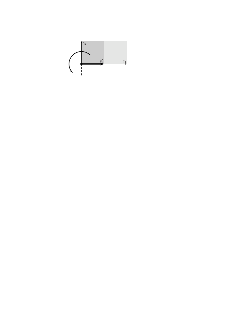
(a) $\mathbbm{T}^{2}/D_{2}$

(b) $\mathbbm{T}^{2}/D_{3}$

Figure 2: Examples of (a) a $\mathbbm{T}^{2}/D_{2}$ and (b) a $\mathbbm{T}^{2}/D_{3}$ orbifold where rank reduction is possible. The action of the dihedral group consists in a rotation by $180^{\circ}$ around the origin, and in a translation by $e_{1}^{\prime}$ in case (a), and a translation by $e_{1}^{\prime\prime}$ or $2\,e_{1}^{\prime\prime}$ in case (b).

These examples can be generalized in the following way: The orbifold can be interpreted as $\mathbbm{O}=\mathbbm{T}^{n}/R$ where $R$ is a symmetry of the lattice, and the torus arises by modding out flat space by discrete translations, $\mathbbm{T}^{n}=\mathbbm{R}^{n}/\Lambda$. By embedding the full symmetry group $K$, containing the operations of $R$ as well as the translations, into the gauge group, it is possible to achieve that the torus $\mathbbm{T}^{n}$, which arises as intermediate step in this picture, carries Wilson lines [34]. Since the generators associated with the Wilson lines do not necessarily commute with the twists corresponding to embedding the operations of $R$ into the gauge group, rank reduction is possible [33]. We believe that similar constructions will be important for model building.

Let us briefly comment on non-regular embeddings. Consider the group $\mathrm{SU}(3)$ which contains $\mathrm{SO}(3)$ (the subgroup of real matrices) as an S-subgroup (in Dynkin’s terminology). Let us pick two generators of the embedded $\mathrm{SO}(3)$, for instance

$$T_{1}\,=\,\left(\begin{array}[]{ccc}0&1&0\\ -1&0&0\\ 0&0&0\end{array}\right)\quad\text{and}\quad T_{2}\,=\,\left(\begin{array}[]{ccc}0&0&-1\\ 0&0&0\\ 1&0&0\end{array}\right)\;.$$ (4.6)

It is then straightforward to convince oneself that imposing the twists $P_{1}=\exp(2\pi\mathrm{i}\,T_{1}/4)$ and $P_{2}=\exp(2\pi\mathrm{i}\,T_{2}/4)$ breaks $\mathrm{SU}(3)$ completely. Similar constructions can be used to break larger groups with only a few twists. For instance, $\mathrm{E}_{8}$ has a maximal S-subalgebra $\mathfrak{su}(2)$ and can therefore be broken completely by only two twists, e.g., by embedding a suitable dihedral group in the $\mathrm{SU}(2)$.

5 Conifold GUTs

We now want to continue the discussion of the generic structure of orbifold GUTs given at the beginning of Sec. 3 and show that a mild generalization of the construction principles leads to a much larger freedom in model building. Our main focus will be on 6d models.

5.1 Geometry and gauge symmetry breaking

In 5 dimensions, the geometry is very constraining. Up to isomorphism, the only smooth compact manifold is $\mathbbm{S}^{1}$, where one has the familiar problems of obtaining chiral matter and of fixing the Wilson line, the value of which represents a modulus which, in the SUSY setting, can not be stabilized by perturbative effects. The only compact orbifold is the interval, which can always be viewed as $\mathbbm{S}^{1}/(\mathbbm{Z}_{2}\times\mathbbm{Z}_{2}^{\prime})$ (with $\mathbbm{S}^{1}/\mathbbm{Z}_{2}$ being a special case). The gauge breaking at each boundary is determined by a $\mathbbm{Z}_{2}$ automorphism and can be interpreted as explicit breaking by boundary conditions. One may try to generalize the setting by considering breaking by a boundary localized Higgs (in the limit where the VEV becomes large) [37] or ascribing Dirichlet and Neumann boundary conditions to different gauge fields (without the $\mathbbm{Z}_{2}$ automorphism restriction) [24]. Furthermore, it is possible to ascribe the breaking to a singular Wilson line crossing the boundary [24]. However, it appears to be unavoidable that geometry is used only in a fairly trivial way and that the breaking is confined entirely to the small-scale physics near the brane, outside the validity range of effective field theory.

Group-theoretically, the 5d setting is also fairly constrained since the relative orientation of the gauge twists at the two boundaries is a modulus. To be more specific, let $P_{1}=\exp({\boldsymbol{T}_{1}})$ and $P_{2}=\exp({\boldsymbol{T}_{2}})$ be the two relevant twists. Even though this makes rank reduction possible in principle, we are faced with the problem that, if the Wilson line connecting the boundaries develops an appropriate VEV, the situation becomes equivalent to both $\boldsymbol{T}_{1}$ and $\boldsymbol{T}_{2}$ being in the Cartan subalgebra, in which case the symmetry is enhanced to a maximal-rank subgroup. SUSY prevents the modulus from being fixed by loop corrections.

In 6 dimensions, the situation is much more complicated and interesting. Clearly, the smooth torus has the same problems as the $\mathbbm{S}^{1}$ discussed above. However, there is a large number of compact manifolds with conical singularities. A simple way to envisage such singular manifolds or, more precisely, conifolds is given in Fig. 3. The fundamental space consists of two identical triangles. The geometry is determined by gluing together the edges of the depicted triangles, thus leading to a triangle with a front and a back, a triangular ‘pillow’. It is flat everywhere except for the three conical singularities corresponding to the three corners of the basic triangle. Each deficit angle is $2(\pi-\varphi)$, where $\varphi$ is the corresponding angle of the triangle. Obviously, in this construction the basic triangle can be replaced by any polygon. If the polygon is non-convex, negative deficit angles appear.

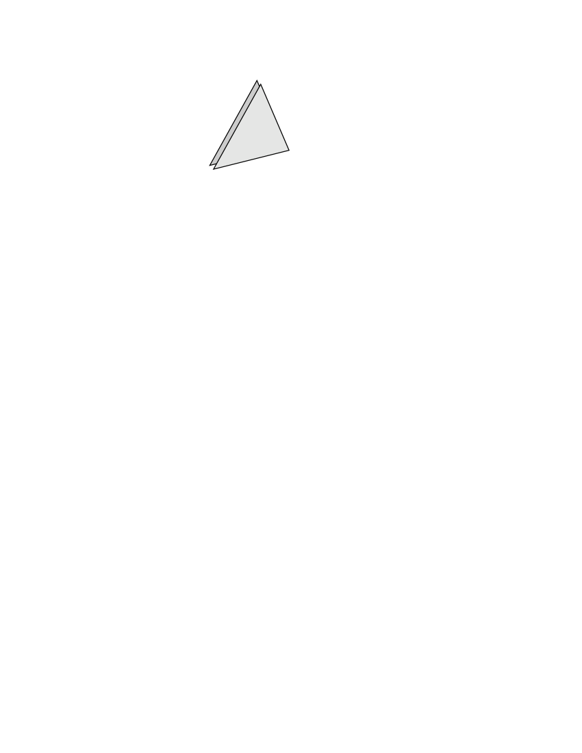
Figure 3: Construction of a compact manifold with singularities from two triangles.

Four specific polygons deserve a separate discussion. These are the rectangle, the equilateral triangle, the isosceles triangle with a $90^{\circ}$ angle, and the triangle with angles $30^{\circ}$, $60^{\circ}$, and $90^{\circ}$. The conifolds constructed in the above manner from these polygons can alternatively be derived from the torus as a $\mathbbm{Z}_{2}$, $\mathbbm{Z}_{3}$, $\mathbbm{Z}_{4}$ and $\mathbbm{Z}_{6}$ orbifold, respectively. Given that $\mathbbm{Z}_{n}$ can not be a symmetry of a 2-dimensional lattice for $n>6$, it is clear that this last method of constructing conifolds is highly constrained when compared to the generic conifold of Fig. 3 with an arbitrary polygon. However, from the perspective of effective field theory model building, there appears to be no fundamental reason to discard the multitude of possibilities arising in the more general framework.

Clearly, even more possibilities open up if, in addition to conical singularities one allows for 1-dimensional boundaries. These arise in orbifolding if a $\mathbbm{Z}_{2}$ reflection symmetry (in contrast to the $\mathbbm{Z}_{n}$ rotation symmetries above) of the torus is modded out [15] (see also [39]). However, in what follows we will concentrate on construction with conical singularities only.

We now turn to the possibilities of geometric gauge symmetry breaking on conifolds. Recall first that, if a given conifold can be constructed from a smooth manifold by modding out a discrete symmetry group, i.e., as an orbifold, then an appropriate embedding of this discrete group into the automorphism group of the gauge Lie algebra will lead to a gauge symmetry reduction. Working directly on the fundamental space (as opposed to the covering space) this gauge breaking can be ascribed to non-trivial values of Wilson lines encircling each of the conical singularities.

It is now fairly obvious how to introduce this type of breaking in the generic construction of Fig. 3 (possibly with the triangle replaced by an arbitrary polygon). First, we identify one edge of the front polygon with the corresponding edge of the back polygon. Next, when identifying along the two adjacent edges, one uses the freedom of introducing a relative gauge twist $P\in G$. In more detail, if $(x,y)$ and $(x^{\prime},y^{\prime})$ parametrize front and back polygon near the relevant edge (such that the edge is at $y=0$ or $y^{\prime}=0$), one demands $A^{\prime}(x^{\prime}=x,y^{\prime}=0)=P\,A(x,y=0)\,P^{-1}$ for the gauge potentials $A$ and $A^{\prime}$ on the two polygons. Continuing with the identifications, one finds that there is a freedom of choosing $n-1$ gauge twists $P_{i}$ in the presence of $n$ conical singularities. Technically, this is due to the fact that the identification along one of the edges can always be made trivial using global gauge rotations of one of the polygons. A geometric understanding follows from the fact that the global topology is that of a sphere, in which case the Wilson lines around $n-1$ singularities fix the last Wilson line (we always assume the vacuum configuration, i.e., $A$ is locally pure gauge).

Clearly, we want to obtain a smooth manifold (except for the singularities) in the end so that, to be more precise, the $P_{i}$ have to be introduced in the appropriate transition functions of the defining atlas. However, we believe that it is not necessary to spell out this familiar construction in detail.

Instead of using only inner automorphisms described by $P_{i}$, we could have allowed for outer automorphisms in the transition functions. In this case, which we will not pursue in this paper, the corresponding vacua are clearly disconnected from those defined only by inner automorphisms. The theory can then be thought of as defined on a generalization of a principal bundle (in the commonly used definition of principal bundles the transition functions involve only inner automorphisms).

We now want to analyze the gauge fields in a small open subset including one conical singularity. A convenient parametrization is given by polar coordinates $(r,\varphi)$ with $0<r<\epsilon$ and $0\leq\varphi<\beta$, where the singularity is at $r=0$ and the deficit angle is $2\pi-\beta$. As familiar from the Hosotani mechanism on smooth manifolds [40], we can trade the gauge twist in the matching from $\varphi=\beta$ to $\varphi=0$ for a background gauge field which, for a twist $P=\exp(\boldsymbol{T})$, can be chosen as $A=\boldsymbol{e}_{\varphi}\boldsymbol{T}/(\beta r)$. Here $\boldsymbol{e}_{\varphi}$ is the unit-vector in $\partial_{\varphi}$ direction so that $A$ is a Lie-algebra-valued vector. This simple exercise demonstrates explicitly that, at least locally, the breaking can be attributed to a non-vanishing gauge field VEV in a flat direction. However, in contrast to the Hosotani mechanism, the corresponding modulus can be fixed without violating the locality assumption (which we consider as fairly fundamental in effective field theory). Namely, the value of the Wilson line described by the above $A$ can be determined by some unspecified small-distance physics directly at the singularity. This is similar to the boundary breaking in 5 dimensions. In contrast to the 5d case, however, the breaking at the conical singularity is visible to the bulk observer, who can encircle the singularity and measure the Wilson line without coming close to the singularity. Thus, one might be tempted to conclude that this type of breaking has a better definition in terms of low-energy effective field theory.

To conclude this subsection, we want to collect the generalizations of 6d field theoretic orbifold models discussed above. First, one can work on conifolds, i.e., use deficit angles that can not result from modding out on the basis of a smooth manifold. The gauge twist at each singularity may, however, be still required to be consistent with the geometric twist. Second, one can insist on conventional orbifolds as far as the geometry is concerned but use arbitrary gauge twists at each conical singularity, i.e., give up the connection between the rotation angles in tangent and gauge space. Third, one may drop both constraints and work on conifolds with arbitrary deficit angles and gauge twists. Obviously, such constructions can also be carried out in more than 6 dimensions. The detailed discussion of those is beyond the scope of the present paper.

5.2 Generating chiral matter

In general, compactification on a non-flat manifold can provide chiral matter if the holonomy group of the compact manifold fulfills certain criteria. For example, it is well-known that compactification of a 10d SYM theory on Calabi-Yau manifolds with $\mathrm{SU}(3)$ holonomy [41] or on orbifolds [9] leads to $N=1$ SUSY in 4d. Both constructions are not unrelated as many orbifolds can be regarded as singular limits of manifolds in which the curvature is concentrated at the fixed points. Since the reduction of SUSY is a matter of geometry, compactification of a higher-dimensional field theory on a conifold can also lead to $N=1$ supersymmetric models in 4d.

Interesting models have been constructed using the fact that the vector multiplet of $N=(1,1)$ SUSY in 6d corresponds to one vector and three chiral multiplets in 4d language, $A=(V,\phi_{1},\phi_{2},\phi_{3})$. The fact that three copies of chiral multiplets appear automatically may be an explanation of the observed number of generations [4]. The above 6d theory can be interpreted as arising from a 10d SYM, in which case the scalars of the chiral multiplets are the extra components of gauge fields [42], for example, $\phi_{1}\ni A_{5}+\mathrm{i}A_{6}$, $\phi_{2}\ni A_{7}+\mathrm{i}A_{8}$ and $\phi_{3}\ni A_{9}+\mathrm{i}A_{10}$ ($A_{M}$ denote the components of the 10d vector). When defining our 6d models, we require the field transformations associated with going around a conical singularity to be an element of an SU(3) subgroup of the full $\mathrm{SO}(6)\simeq\mathrm{SU}(4)$ symmetry of the underlying 10d SYM theory. Under this subgroup, which we call $\mathrm{SU}(3)$ R-symmetry, the chiral superfields $\phi_{i}$ transform as a $\boldsymbol{3}$. The appealing feature of such a construction is that matter multiplets are not put in ‘by hand’ but arise in a natural way from a higher-dimensional SYM theory [5, 4, 7, 6].

The action of the $\mathrm{SU}(3)$ R-symmetry transformation on the chiral superfields is not completely arbitrary. For example, if $\phi_{1}\ni A_{5}+\mathrm{i}A_{6}$, the transformation of $\phi_{1}$ is fixed by geometry, e.g., when modding out a rotation symmetry, a corresponding rotation has to be applied to the $\phi_{1}$ superfield. Thus, when going around a conical singularity, $\phi_{1}$ receives a phase which is given by $2\varphi$, where $\varphi$ is the corresponding angle of the polygon. Since multiplying by the phase $e^{\mathrm{i}2\varphi}$ corresponds to a rotation in the complex plane, we will call $2\varphi$ ‘rotation angle’ in what follows. Clearly, the rotation angle sums up with the deficit angle to $2\pi$.

6 Specific models

Let us now discuss three models in which some of the main features of the last sections are exemplified. All these models are based on a SYM theory in $4+2$ dimensions endowed with $(N_{1},N_{2})=(1,1)$ SUSY. In 4d we then deal with three chiral superfields $\phi_{1}$, $\phi_{2}$ and $\phi_{3}$ where we assume that $\phi_{1}=A_{5}+\mathrm{i}A_{6}$ so that the action of the R-symmetry on $\phi_{1}$ is fixed (cf. Sec. 5.2).

6.1 $\boldsymbol{\mathrm{E}_{7}\to\mathrm{SU}(5)\times\mathrm{SU}(3)_{\mathrm{F}}\times\mathrm{U}(1)}$

Consider a SYM theory based on an $\mathrm{E}_{7}$ gauge group. $\mathrm{E}_{7}$ contains $\mathrm{SU}(5)\times\mathrm{SU}(3)_{\mathrm{F}}\times\mathrm{U}(1)$, and the adjoint representation decomposes as

$$\boldsymbol{133} \to (\boldsymbol{24},\boldsymbol{1})_{0}\oplus(\boldsymbol{1},\boldsymbol{1})_{0}\oplus(\boldsymbol{1},\boldsymbol{8})_{0}\oplus(\boldsymbol{5},\boldsymbol{1})_{6}\oplus(\overline{\boldsymbol{5}},\boldsymbol{1})_{-6}$$ (6.1)

$${}\oplus(\boldsymbol{10},\overline{\boldsymbol{3}})_{-2}\oplus(\overline{\boldsymbol{5}},\boldsymbol{3})_{-4}\oplus(\overline{\boldsymbol{10}},\boldsymbol{3})_{2}\oplus(\boldsymbol{5},\overline{\boldsymbol{3}})_{4}\;,$$

where we use a notation analogous to Eq. (3.10).

As explained in Sec. 3, the twist $P$ which causes the desired breaking can be understood as exponential of the $\mathrm{U}(1)$ generator. Under this twist, the multiplets appearing in Eq. (6.1) acquire phases which are proportional to the $\mathrm{U}(1)$ charge. By taking the proportionality constant to be $-1/12$, we arrive at the phases listed in Tab. 6.1 where here and below phases are given in units of $2\pi$.

$\begin{array}[]{|rcl|rcl|rcl|}\hline\cr(\boldsymbol{24},\boldsymbol{1})_{0}&:&\boldsymbol{0}&(\boldsymbol{5},\boldsymbol{1})_{6}&:&\boldsymbol{1/2}&(\overline{\boldsymbol{5}},\boldsymbol{3})_{-4}&:&\boldsymbol{1/3}\vphantom{\overline{\overline{\boldsymbol{5}}}}\\ (\boldsymbol{1},\boldsymbol{1})_{0}&:&\boldsymbol{0}&(\overline{\boldsymbol{5}},\boldsymbol{1})_{-6}&:&\boldsymbol{1/2}&(\overline{\boldsymbol{10}},\boldsymbol{3})_{2}&:&5/6\\ (\boldsymbol{1},\boldsymbol{8})_{0}&:&\boldsymbol{0}&(\boldsymbol{10},\overline{\boldsymbol{3}})_{-2}&:&\boldsymbol{1/6}&(\boldsymbol{5},\overline{\boldsymbol{3}})_{4}&:&2/3\\ \hline\cr\end{array}$

Table 6.1: Phases (in units of $2\pi$) for the different multiplets of $\mathrm{SU}(5)\times\mathrm{SU}(3)_{\mathrm{F}}\times\mathrm{U}(1)\subset\mathrm{E}_{7}$. Zeros correspond to the surviving gauge bosons, other phases which are compensated by the R-symmetry transformations are written in boldface.

The smallest phase present is $1/6$ so that $P$ is a $\mathbbm{Z}_{6}$ twist. Therefore, the R-symmetry acts on $\phi_{1}$ as a $-60^{\circ}$ rotation in the 5-6 plane, and thus the $(\boldsymbol{10},\overline{\boldsymbol{3}})_{-2}$ possesses a zero-mode. We choose the transformation of $\phi_{2}$ such that the $(\overline{\boldsymbol{5}},\boldsymbol{3})_{-4}$ survives as well, and the phase of $\phi_{3}$ is then fixed by the determinant condition. More explicitly, by taking

$$R\,=\,\exp[2\pi\mathrm{i}\,\operatorname{diag}(-1/6,2/3,-1/2)]\;\in\mathrm{SU}(3)\;,$$ (6.2)

we can achieve that 3 generations of $\boldsymbol{10}$ and $\overline{\boldsymbol{5}}$ survive without any mirrors, indicated by boldface phases in Tab. 6.1, and an $N=1$ SUSY in 4d is preserved. It is also interesting to observe that the only additional surviving superfields, namely $(\boldsymbol{5},\boldsymbol{1})_{6}$ and $(\overline{\boldsymbol{5}},\boldsymbol{1})_{-6}$ which acquire phases $1/2$ and therefore have zero-modes due to the third diagonal entry of $R$, carry the quantum numbers of the light Higgs fields in the supersymmetric $\mathrm{SU}(5)$ theory. Thus, the $\mathrm{SU}(5)$ part of this model looks relevant for reality, and is in particular anomaly-free.

The geometry of this model, which can be constructed as a standard orbifold $\mathbbm{T}^{2}/\mathbbm{Z}_{6}$, is given by two triangles with angles $30^{\circ}$, $60^{\circ}$ and $90^{\circ}$ (cf. Fig. 4). The $\mathbbm{Z}_{6}$ twist $P$ ($P_{6}=P$ in Fig. 4) is associated with the first of these fixed points; the twists $P^{2}$ and $P^{3}$ are associated with the remaining two fixed points. By construction, the order of rotation in the two extra dimensions coincides with the order of the twist in the gauge group.

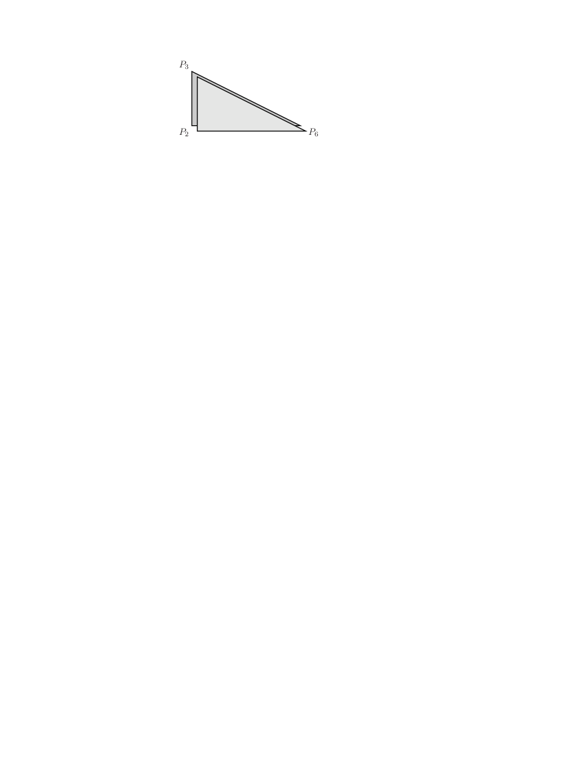
Figure 4: Example of a $4+2$ dimensional orbifold allowing for $\mathbbm{Z}_{6}$ twists. The fundamental space consists of two triangles. The geometry can be illustrated by gluing together the edges of the depicted triangles, thus leading to a triangle with a front- and a backside.

It is then straightforward to determine the gauge groups which survive at these fixed points. In the actual example, they turn out to be $\mathrm{SU}(6)\times\mathrm{SU}(3)_{\mathrm{F}}$ and $\mathrm{SU}(8)$, respectively. The content of non-vanishing fields at these fixed points is also found to be anomaly-free under the relevant surviving gauge group in both cases, which implies the absence of localized anomalies [44].

The complete model is, however, not free of anomalies. This is due to localized anomalies at the $P_{6}$ fixed points, where the gauge group is SU(5)$\times$U(1)$\times\mathrm{SU}(3)_{\mathrm{F}}$. However, the SU(5) part by itself is free of localized anomalies even at this fixed point. Thus, if $\mathrm{SU}(3)_{\mathrm{F}}\times\mathrm{U}(1)$ is broken, as it has to be in order to describe reality, there are no anomalies. The desired breaking of the unwanted symmetries may be due to fields which live on the fixed points, however, discussing such possibilities is beyond the scope of this study. Note also that if we were to break the additional symmetry by rank-reducing twists, fewer matter fields would survive. That is also the reason why we do not use rank-reducing twists in the next two models.

6.2 $\boldsymbol{\mathrm{E}_{8}\to G_{\mathrm{PS}}\times\mathrm{U}(1)^{3}}$

Under $\mathrm{E}_{8}\to\mathrm{SO}(10)\times\mathrm{SU}(4)$, the adjoint representation of $\mathrm{E}_{8}$ decomposes like

$$\boldsymbol{248}\,\to\,(\boldsymbol{45},\boldsymbol{1})\oplus(\boldsymbol{1},\boldsymbol{15})\oplus(\boldsymbol{16},\boldsymbol{4})\oplus(\overline{\boldsymbol{16}},\overline{\boldsymbol{4}})\oplus(\boldsymbol{10},\boldsymbol{6})\;.$$ (6.3)

$\mathrm{SO}(10)$ contains the Pati-Salam group [3] $G_{\mathrm{PS}}=\mathrm{SU}(4)\times\mathrm{SU}(2)\times\mathrm{SU}(2)$ whereby

$$\boldsymbol{45} \to (\boldsymbol{15},\boldsymbol{1},\boldsymbol{1})\oplus(\boldsymbol{1},\boldsymbol{3},\boldsymbol{1})\oplus(\boldsymbol{1},\boldsymbol{1},\boldsymbol{3})\oplus(\boldsymbol{6},\boldsymbol{2},\boldsymbol{2})\;,$$ (6.4a)

$$\boldsymbol{16} \to (\boldsymbol{4},\boldsymbol{2},\boldsymbol{1})\oplus(\overline{\boldsymbol{4}},\boldsymbol{1},\boldsymbol{2})\;,$$ (6.4b)

$$\boldsymbol{10} \to (\boldsymbol{6},\boldsymbol{1},\boldsymbol{1})\oplus(\boldsymbol{1},\boldsymbol{2},\boldsymbol{2})\;.$$ (6.4c)

This breaking can be achieved by using the rotation $-\mathbbm{1}\in\mathrm{SU}(2)$ for the first (or the second) $\mathrm{SU}(2)$. In addition, we can now impose the twist

$$F\,=\,\exp\left[2\pi\,\mathrm{i}\,\operatorname{diag}\left(1/3,-1/6,x,-1/6-x\right)\right]\in\mathrm{SU}(4)\;,$$ (6.5)

where, e.g., $x=\frac{1}{4}$, in order to break $\mathrm{SU}(4)\to[\mathrm{U}(1)]^{3}$. The charges of the $\boldsymbol{4}$ are then given by $q_{i}\in\{1/3,-1/6,x,-1/6-x\}$. The charges of the $\boldsymbol{6}$ are $q_{i}+q_{j}$ with $i\neq j$ since the $\boldsymbol{6}$ is the antisymmetric part of the $\boldsymbol{4}\times\boldsymbol{4}$ of $\mathrm{SU}(4)$, and finally the charges of the $\boldsymbol{15}$ are $q_{i}-q_{j}$.

Together with the R-symmetry transformation

$$R\,=\,\exp\left[2\pi\mathrm{i}\,\operatorname{diag}\left(-1/3,-1/3,-1/3\right)\right]\;,$$ (6.6)

three chiral generations of matter and three Higgs, i.e., $(\boldsymbol{1},\boldsymbol{2},\boldsymbol{2})$, survive. Only for certain $x$, additional fields will possess zero-modes, and we will choose $x$ to equal none of these values. Here, the number of generations is due to dimensional reduction of $(N_{1},N_{2})=(1,1)$ SUSY in 6d to 4d. The surviving gauge group is $G_{\mathrm{PS}}\times[\mathrm{U}(1)]^{3}$. The geometry is given by an equilateral triangle with the three corners corresponding to three identical fixed points.

Obviously, for such a construction, the geometric twist, i.e., the rotation in the two extra dimensions, is of a lower order than the group theoretical twist. This requires going beyond the usual field-theoretic orbifold constructions (although the geometry is still an orbifold). As proposed in Sec. 5, we define a field theory on a manifold with three conical singularities, each of them possessing a deficit angle of $2\pi/3$. This construction is then an equilateral triangle. We then add Wilson lines such that the group-theoretical twist $P$ at two of the fixed points equals the one described above. The twist at the third fixed point is then constrained to be $P^{-2}$ by the global geometry.

At each singularity of the conifold, the Pati-Salam part of the gauge group is anomaly-free. This is obvious for first two fixed points since the non-vanishing fields are those of the standard model with three Higgs doublets. At the third fixed point, the gauge symmetry is enhanced to the group SO(10), which has no 4d anomalies. Again, investigating mechanisms to break the extra $\mathrm{U}(1)$s as well as $G_{\mathrm{PS}}$ to $G_{\mathrm{SM}}$ is beyond the scope of this paper.

Note finally that this particular model can be viewed as an extension of [4], where three generations arise from the three chiral superfields present in the 4d description of a 10d SYM theory, i.e., they follow from the presence of three complex extra dimensions. The new points in our construction are the doublet-triplet splitting solution arising from the breaking to the Pati-Salam group (see [48] and the recent related stringy models of [49]) and the realization of all rather than just part of the matter fields in terms of the SYM multiplet.

6.3 $\boldsymbol{\mathrm{E}_{8}\to G_{\mathrm{PS}}\times\mathrm{SU}(3)_{\mathrm{F}}\times\mathrm{U}(1)}$

Alternatively, we can obtain $G_{\mathrm{PS}}$ from $\mathrm{E}_{8}$ and maintain an $\mathrm{SU}(3)_{\mathrm{F}}$ flavour symmetry by breaking the extra $\mathrm{SU}(4)$ of the decomposition (6.3) to $\mathrm{SU}(3)_{\mathrm{F}}\times\mathrm{U}(1)$. In order to achieve this breaking, we take a central element of $\mathrm{SU}(3)$,

$$P\,=\,\exp\left[2\pi\mathrm{i}\,\left(1/3,1/3,1/3,0\right)\right]\;.$$ (6.7)

The phases which arise by combining this twist with $\exp(-2\pi\mathrm{i}/4\,\mathbbm{1})\in\mathrm{SU}(4)$ are listed in Tab. 6.2.

$$\begin{array}[]{|rcl|rcl|rcl|}\hline\cr&&&&&&&&\\[-8.5359pt] (\boldsymbol{15},\boldsymbol{1},\boldsymbol{1};\boldsymbol{1}_{0})&:&\boldsymbol{0}&(\boldsymbol{1},\boldsymbol{1},\boldsymbol{1};\overline{\boldsymbol{3}}_{-4/3})&:&2/3&(\overline{\boldsymbol{4}},\boldsymbol{1},\boldsymbol{2};\overline{\boldsymbol{3}}_{-1})&:&11/12\\ (\boldsymbol{1},\boldsymbol{3},\boldsymbol{1};\boldsymbol{1}_{0})&:&\boldsymbol{0}&(\boldsymbol{4},\boldsymbol{2},\boldsymbol{1};\boldsymbol{3}_{1})&:&\boldsymbol{1/12}&(\overline{\boldsymbol{4}},\boldsymbol{1},\boldsymbol{2};\boldsymbol{1}_{-3})&:&1/4\\ (\boldsymbol{1},\boldsymbol{1},\boldsymbol{3};\boldsymbol{1}_{0})&:&\boldsymbol{0}&(\boldsymbol{4},\boldsymbol{2},\boldsymbol{1};\boldsymbol{1}_{-3})&:&3/4&(\boldsymbol{6},\boldsymbol{1},\boldsymbol{1};\boldsymbol{3}_{1})&:&5/6\\ (\boldsymbol{1},\boldsymbol{1},\boldsymbol{1};\boldsymbol{8}_{0})&:&\boldsymbol{0}&(\overline{\boldsymbol{4}},\boldsymbol{1},\boldsymbol{2};\boldsymbol{3}_{1})&:&\boldsymbol{7/12}&(\boldsymbol{6},\boldsymbol{1},\boldsymbol{1};\overline{\boldsymbol{3}}_{-1})&:&1/6\\ (\boldsymbol{1},\boldsymbol{1},\boldsymbol{1};\boldsymbol{1}_{0})&:&\boldsymbol{0}&(\overline{\boldsymbol{4}},\boldsymbol{1},\boldsymbol{2};\boldsymbol{1}_{3})&:&1/4&(\boldsymbol{1},\boldsymbol{2},\boldsymbol{2};\boldsymbol{3}_{1})&:&\boldsymbol{1/3}\\ (\boldsymbol{6},\boldsymbol{2},\boldsymbol{2};\boldsymbol{1}_{0})&:&1/2&(\boldsymbol{4},\boldsymbol{2},\boldsymbol{1};\overline{\boldsymbol{3}}_{-1})&:&11/12&(\boldsymbol{1},\boldsymbol{2},\boldsymbol{2};\overline{\boldsymbol{3}}_{-1})&:&2/3\\ (\boldsymbol{1},\boldsymbol{1},\boldsymbol{1};\boldsymbol{3}_{4/3})&:&\boldsymbol{1/3}&(\boldsymbol{4},\boldsymbol{2},\boldsymbol{1};\boldsymbol{1}_{3})&:&3/4&&&\\ \hline\cr\end{array}$$

Table 6.2: Table of the phase factors for the different multiplets of $G_{\mathrm{PS}}\times\mathrm{SU}(3)_{\mathrm{F}}\times\mathrm{U}(1)\subset\mathrm{E}_{8}$. Zeros correspond to surviving gauge bosons; other phases which are compensated by the R-symmetry transformation are written in boldface.

Now let us simultaneously impose an R-symmetry twist

$$R\,=\,\exp\left[2\pi\mathrm{i}\,\operatorname{diag}(-1/12,-7/12,-1/3)\right]\;.$$ (6.8)

It is then easy to see from Tab. 6.2 that the zero modes which emerge in the matter sector are three generations of SM matter, three Higgs and three additional neutrinos.

In order to realize such a model, we have again to relax the constraints of usual orbifold models, and therefore consider a manifold with a conical singularity with deficit angle $2\pi\cdot 5/12$ instead (cf. Sec. 5). To be more specific, we envisage the geometry of the model as an isosceles triangle with an angle of $2\pi\cdot 5/12$. Each corner corresponds to a fixed point, and we are free to choose both $\pi/12$ fixed points identically. By construction, the group-theoretical twist $P$ at the $\pi/12$ fixed points generate a $\mathbbm{Z}_{12}$, i.e., $P^{12}=\mathbbm{1}$. At the remaining $2\pi\cdot 5/12$ ‘corner’, we choose the twist $P^{10}=P^{-2}$ for consistency. Interestingly, a quick inspection of Tab. 6.2 reveals that the there surviving gauge symmetry is $\mathrm{SO}(10)$. Obviously, the $\mathrm{SO}(10)$ part of the gauge theory at this fixed point is anomaly-free automatically.

Once more, discussing the breaking of the extra gauge symmetry is beyond the scope of this study.

7 Conclusions

We have explored some of the group-theoretical possibilities in orbifold GUTs. In particular, we showed that, given a simple gauge group $G$, the breaking to any maximal-rank regular subgroup can be achieved by orbifolding.

We further studied rank reduction and found that simple group factors can always be broken completely. This is possible when using non-Abelian twists, and also if twists commute but the corresponding generators do not. Using such constructions in orbifolding is made possible by embedding a non-Abelian (or even Abelian) space group into the gauge group.

We then extended the familiar concept of orbifold GUTs by replacing the orbifolds by manifolds with conical singularities. The possibilities we discussed include orbifold geometries endowed with unrestricted Wilson lines wrapping the conical singularities, manifolds with conical singularities with arbitrary deficit angles, and combinations thereof.

Finally, we presented three specific models where three generations of fields carrying the SM quantum numbers come from a SYM theory in 6d. While the first one is a conventional orbifold model illustrating the usefulness of our group theoretical methods, the two others are based on the two new concepts mentioned above.

To summarize, we explored several new and interesting methods and possibilities which can be used in orbifold GUTs and their generalizations.

As none of our models is yet completely realistic, more effort is required in order to discuss phenomenological consequences. However, it is very appealing how easily three generations can be obtained and the doublet-triplet splitting problem can be solved. Thus, promoting our models to realistic ones in future studies appears to be worthwhile.

Note added: While this paper was being finalized, Ref. [50] appeared where Dynkin diagram techniques were used as well. Aspects of our analysis not addressed by [50] include, in particular, the breaking of any simple group to all maximal-rank regular subgroups, rank-reduction, as well as several new field-theoretic concepts and models.

A Table of orbifold twists

Group	Twist	Symmetric subgroup	Comment
$\mathrm{SU}(N+M)$	$\mathbbm{Z}_{2}$	$\mathrm{SU}(N)\times\mathrm{SU}(M)\times\mathrm{U}(1)$
$\mathrm{SO}(N+M)$	$\mathbbm{Z}_{2}$	$\mathrm{SO}(N)\times\mathrm{SO}(M)$	$N$ or $M$ even
$\mathrm{SO}(2N)$	$\mathbbm{Z}_{2}$	$\mathrm{SU}(N)\times\mathrm{U}(1)$
$\mathrm{Sp}(2N+2M)$	$\mathbbm{Z}_{2}$	$\mathrm{Sp}(2N)\times\mathrm{Sp}(2M)$
$\mathrm{Sp}(2N)$	$\mathbbm{Z}_{2}$	$\mathrm{SU}(N)\times\mathrm{U}(1)$
$\mathrm{G}_{2}$	$\mathbbm{Z}_{2}$	$\mathrm{SU}(2)\times\mathrm{SU}(2)$
$\mathrm{G}_{2}$	$\mathbbm{Z}_{3}$	$\mathrm{SU}(3)$
$\mathrm{F}_{4}$	$\mathbbm{Z}_{2}$	$\mathrm{Sp}(6)\times\mathrm{SU}(2)$
$\mathrm{F}_{4}$	$\mathbbm{Z}_{3}$	$\mathrm{SU}(3)\times\mathrm{SU}(3)$
$\mathrm{F}_{4}$	$\mathbbm{Z}_{4}$	$\mathrm{SU}(4)\times\mathrm{SU}(2)$	not maximal
$\mathrm{F}_{4}$	$\mathbbm{Z}_{2}$	$\mathrm{SO}(9)$
$\mathrm{E}_{6}$	$\mathbbm{Z}_{2}$	$\mathrm{SO}(10)\times\mathrm{U}(1)$
$\mathrm{E}_{6}$	$\mathbbm{Z}_{2}$	$\mathrm{SU}(6)\times\mathrm{SU}(2)$
$\mathrm{E}_{6}$	$\mathbbm{Z}_{3}$	$\mathrm{SU}(3)\times\mathrm{SU}(3)\times\mathrm{SU}(3)$
$\mathrm{E}_{7}$	$\mathbbm{Z}_{2}$	$\mathrm{SO}(12)\times\mathrm{SU}(2)$
$\mathrm{E}_{7}$	$\mathbbm{Z}_{3}$	$\mathrm{SU}(6)\times\mathrm{SU}(3)$
$\mathrm{E}_{7}$	$\mathbbm{Z}_{4}$	$\mathrm{SU}(4)\times\mathrm{SU}(4)\times\mathrm{SU}(2)$	not maximal
$\mathrm{E}_{7}$	$\mathbbm{Z}_{2}$	$\mathrm{E}_{6}\times\mathrm{U}(1)$
$\mathrm{E}_{7}$	$\mathbbm{Z}_{2}$	$\mathrm{SU}(8)$
$\mathrm{E}_{8}$	$\mathbbm{Z}_{2}$	$\mathrm{SO}(16)$
$\mathrm{E}_{8}$	$\mathbbm{Z}_{4}$	$\mathrm{SU}(8)\times\mathrm{SU}(2)$	not maximal
$\mathrm{E}_{8}$	$\mathbbm{Z}_{6}$	$\mathrm{SU}(6)\times\mathrm{SU}(3)\times\mathrm{SU}(2)$	not maximal
$\mathrm{E}_{8}$	$\mathbbm{Z}_{5}$	$\mathrm{SU}(5)\times\mathrm{SU}(5)$
$\mathrm{E}_{8}$	$\mathbbm{Z}_{4}$	$\mathrm{SO}(10)\times\mathrm{SU}(4)$	not maximal
$\mathrm{E}_{8}$	$\mathbbm{Z}_{3}$	$\mathrm{E}_{6}\times\mathrm{SU}(3)$
$\mathrm{E}_{8}$	$\mathbbm{Z}_{2}$	$\mathrm{E}_{7}\times\mathrm{SU}(2)$
$\mathrm{E}_{8}$	$\mathbbm{Z}_{3}$	$\mathrm{SU}(9)$

Table A.1: Maximal subgroups of the simple groups and the corresponding $\mathbbm{Z}_{n}$ orbifold twists. The five non-maximal subgroups which can be obtained by removing one node of the extended Dynkin diagram are listed for the sake of completeness.

References

- [1] H. Georgi and S. Glashow, Phys. Rev. Lett. 32 (1974) 438.
-
[2]
H. Georgi, AIP Conf. Proc. 23 (1975) 575;
H. Fritzsch and P. Minkowski, Annals Phys. 93 (1975) 193. -
[3]
J. Pati and A. Salam, Phys. Rev. D8 (1973) 1240;
J. Pati and A. Salam, Phys. Rev. D10 (1974) 275. - [4] T. Watari and T. Yanagida, Phys. Lett. B 532 (2002) 252 [arXiv:hep-ph/0201086].
-
[5]
K. S. Babu, S. M. Barr and B. s. Kyae,
Phys. Rev. D 65 (2002) 115008
[arXiv:hep-ph/0202178]. - [6] G. Burdman and Y. Nomura, Nucl. Phys. B 656 (2003) 3 [arXiv:hep-ph/0210257].
- [7] I. Gogoladze, Y. Mimura and S. Nandi, arXiv:hep-ph/0304118.
- [8] E. Witten, Nucl. Phys. B 258 (1985) 75.
- [9] L. J. Dixon, J. A. Harvey, C. Vafa and E. Witten, Nucl. Phys. B 261 (1985) 678 and 274 (1986) 285.
- [10] Y. Kawamura, Prog. Theor. Phys. 105 (2001) 999 [arXiv:hep-ph/0012125].
- [11] G. Altarelli and F. Feruglio, Phys. Lett. B 511 (2001) 257 [arXiv:hep-ph/0102301].
- [12] L. J. Hall and Y. Nomura, Phys. Rev. D 64 (2001) 055003 [arXiv:hep-ph/0103125].
-
[13]
A. Hebecker and J. March-Russell, Nucl. Phys. B 613 (2001) 3
[arXiv:hep-ph/0106166]. -
[14]
T. Asaka, W. Buchmüller and L. Covi, Phys. Lett. B 523 (2001) 199
[arXiv:hep-ph/0108021]. - [15] L. J. Hall, Y. Nomura, T. Okui and D. R. Smith, Phys. Rev. D 65 (2002) 035008 [arXiv:hep-ph/0108071].
-
[16]
E. B. Dynkin, The structure of semi-simple algebras,
Amer. Math. Soc. Transl. No. 1 (1950) pp. 1-143,
also Amer. Math. Soc. Transl. (1) 9 (1962) pp. 328-469. - [17] E. B. Dynkin, Semi-simple subalgebras of semi-simple Lie algebras, Amer. Math. Soc. Transl., Ser. 2, 6 (1957) pp. 111-244.
- [18] E. B. Dynkin, Maximal subgroups of the classical groups, Amer. Math. Soc. Transl., Ser. 2, 6 (1957) pp. 245-378.
- [19] E. B. Dynkin, Selected papers, Amer. Math. Soc., 1999.
-
[20]
R. Gilmore, Lie groups, Lie algebras, and some of their applications,
Malabar Krieger, 1994. -
[21]
R. N. Cahn, Semisimple Lie algebras and their representations,
Benjamin/Cummings, 1984. - [22] H. Georgi, Lie algebras in particle physics. From isospin to unified theories, 2nd edition, vol. 54, Perseus Books, 1999.
- [23] R. Slansky, Phys. Rept. 79 (1981) 1.
-
[24]
A. Hebecker and J. March-Russell, Nucl. Phys. B625 (2002) 128
[arXiv:hep-ph/0107039]. - [25] N. Haba, M. Harada, Y. Hosotani and Y. Kawamura, Nucl. Phys. B 657 (2003) 169 [arXiv:hep-ph/0212035].
-
[26]
L. J. Hall and Y. Nomura, arXiv:hep-ph/0212134;
M. Quiros, arXiv:hep-ph/0302189. - [27] H. D. Fegan, An introduction to compact Lie groups, World Scientific Publishing, 1991, 131 P.
-
[28]
K. R. Dienes and J. March-Russell,
Nucl. Phys. B 479 (1996) 113
[arXiv:hep-th/9604112]. -
[29]
Y. Katsuki, Y. Kawamura, T. Kobayashi, N. Ohtsubo and K. Tanioka, Prog. Theor. Phys. 82 (1989) 171.
Y. Katsuki, Y. Kawamura, T. Kobayashi, N. Ohtsubo, Y. Ono and K. Tanioka, Nucl. Phys. B 341 (1990) 611. - [30] M. Golubitsky and B. Rothschild, Primitive subalgebras of exceptional Lie algebras, Pac. J. Math. 39 No. 2 (1971), 371–393.
-
[31]
T. Asaka, W. Buchmüller and L. Covi, Phys. Lett. B 540 (2002) 295
[arXiv:hep-ph/0204358]. - [32] N. Haba and Y. Shimizu, arXiv:hep-ph/0212166.
- [33] L. E. Ibanez, H. P. Nilles and F. Quevedo, Phys. Lett. B 192 (1987) 332.
- [34] L. E. Ibanez, H. P. Nilles and F. Quevedo, Phys. Lett. B 187 (1987) 25.
- [35] E. P. Wigner, Group theory, Academic press, 1949, 372 P.
- [36] S. Groot Nibbelink, arXiv:hep-th/0305139.
-
[37]
Y. Nomura, D. R. Smith and N. Weiner, Nucl. Phys. B 613 (2001) 147
[arXiv:hep-ph/0104041]. - [38] A. Hebecker, Nucl. Phys. B 632 (2002) 101 [arXiv:hep-ph/0112230].
- [39] T. j. Li, Nucl. Phys. B 633 (2002) 83 [arXiv:hep-th/0112255].
- [40] Y. Hosotani, Phys. Lett. B 126 (1983) 309, and Annals Phys. 190 (1989) 233.
- [41] P. Candelas, G. T. Horowitz, A. Strominger and E. Witten, Nucl. Phys. B 258 (1985) 46.
- [42] N. Marcus, A. Sagnotti and W. Siegel, Nucl. Phys. B 224 (1983) 159.
-
[43]
Y. Imamura, T. Watari and T. Yanagida,
Phys. Rev. D 64 (2001) 065023
[arXiv:hep-ph/0103251]. -
[44]
T. Asaka, W. Buchmüller and L. Covi, Nucl. Phys. B 648 (2003) 231
[arXiv:hep-ph/0209144]. - [45] F. Gmeiner, S. Groot Nibbelink, H. P. Nilles, M. Olechowski and M. G. Walter, Nucl. Phys. B 648 (2003) 35 [arXiv:hep-th/0208146].
- [46] G. von Gersdorff and M. Quiros, arXiv:hep-th/0305024.
- [47] A. E. Faraggi, talk at 4th Int. Conf. on Phys. Beyond the Standard Model, Lake Tahoe, 1994 [arXiv:hep-ph/9501288].
-
[48]
R. Dermisek and A. Mafi, Phys. Rev. D 65 (2002) 055002
[arXiv:hep-ph/0108139];
H. D. Kim and S. Raby, JHEP 0301 (2003) 056 [arXiv:hep-ph/0212348]. -
[49]
J. E. Kim, arXiv:hep-th/0301177;
K. S. Choi and J. E. Kim, arXiv:hep-ph/0305002. - [50] K. S. Choi, K. Hwang and J. E. Kim, arXiv:hep-th/0304243.