Abstract

We consider a special class of dimension-six operators which are assumed to be induced by some new physics with typical scales of order $\Lambda$. This special class are the operators with two quarks which can mediate transitions between quark flavours. We show that under quite general assumptions the effect of these operators can be parametrised in terms of six parameters, leading to a modification of the (at tree level flavour diagonal) neutral currents and to an “effective CKM matrix” for the charged currents, which is not necessarily unitary any more. The effects of these operators on charged and neutral currents are studied.

1 Introduction

In the coming few years the flavour sector of the standard model (SM) will have to pass its first detailed test, which hopefully leads to some hint to physics beyond the SM. Being the most general renormalizable theory compatible with the observed broken $SU(3)_{C}\times SU(2)_{L}\times U(1)_{Y}$ symmetry and the observed particle spectrum, any effect beyond the SM has to show up at the scale of the weak boson masses as a set of operators with mass dimension of six or higher, where these operators have to be compatible with the SM symmetry. The coupling constants of the dimension-six operators scale as $1/\Lambda^{2}$ where $\Lambda$ represents the scale of the new physics.

All the possible operators have been listed already some time ago [1], but due to their large number this approach is - in its full generality - useless for phenomenological applications, since every operator comes with an unknown coupling constant. Thus it is unavoidable to restrict their number by some assumption. As an example one can consider the parametrisation of new-physics effects in terms of the Peskin-Takeuchi parameters $S$, $T$ and $U$ [2] which have been used in the analysis of the LEP precision data. These parameters can be related to a certain subset of dimension-six operators [3] and are thus an example for a generic analysis.

However, up to now flavour physics lacks such a simple parametrisation of new-physics effects. Looking at the list of dimension-six operators which can appear at the scale of the weak bosons only those with quark fields are relevant for flavour physics. These operators have either four quark fields (in which case there are no other fields) or two quark fields, in which case the remaining three mass dimensions are made up by either covariant derivatives or Higgs fields.

A specific feature of the SM is the significant suppression of neutral currents by the GIM mechanism, making neutral current transitions very sensitive to possible new-physics effects. This has been investigated before in a number of publications; see eg. [4, 5]. However, the symmetries of the SM suggest that one could also have effects in the charged currents, where the SM effects are at best CKM suppressed and thus one has less sensitivity to new-physics effects.

In the present paper we discuss the impact of dimension-six two-quark operators, which could be induced at the scale of the weak bosons by some new-physics effect. We are aiming at a simple phenomenological parametrisation in the spirit of the aforementioned analysis of the gauge sector by Peskin and Takeuchi. A similar aaproach has been suggested recently for the Higgs sector [6].

In the next section we classify the general dimension-six operators which are relevant at the scale of the weak boson mass, which are bilinear in the quark fields and which are compatible with the symmetries of the SM. We make well defined simplifying assumptions that restrict the number of parameters to only 6. Finally we discuss our result and conclude.

2 Dimension-Six Operators

We shall first write down the standard model contributions in order to fix our notation. Starting from a $SU(2)_{L}\times SU(2)_{R}$ symmetry we group the left-handed quarks according to

$$Q_{1}=\left(\begin{array}[]{c}u_{L}\\ d_{L}\end{array}\right)\quad Q_{2}=\left(\begin{array}[]{c}c_{L}\\ s_{L}\end{array}\right)\quad Q_{3}=\left(\begin{array}[]{c}t_{L}\\ b_{L}\end{array}\right)$$ (1)

and likewise for the right-handed quarks

$$q_{1}=\left(\begin{array}[]{c}u_{R}\\ d_{R}\end{array}\right)\quad q_{2}=\left(\begin{array}[]{c}c_{R}\\ s_{R}\end{array}\right)\quad q_{3}=\left(\begin{array}[]{c}t_{R}\\ b_{R}\end{array}\right)$$ (2)

such that $Q_{A}$ transforms as a $(2,1)$ and $q_{A}$ as a $(1,2)$ under $SU(2)_{L}\times SU(2)_{R}$.

The Higgs field transforms as a $(2,2)$ under this symmetry and we gather the two real fields $\phi_{0}$, $\chi_{0}$ and the complex field $\phi_{+}=\phi_{-}^{*}$ into a $2\times 2$ matrix

$$H=\frac{1}{\sqrt{2}}\left(\begin{array}[]{cc}\phi_{0}-i\chi_{0}&\ \sqrt{2}\phi_{+}\\ -\sqrt{2}\phi_{-}&\ \phi_{0}+i\chi_{0}\end{array}\right)\,.$$ (3)

We can now write down the Lagrangian for a non-linear sigma model, having an $SU(2)_{L}\times SU(2)_{R}$ symmetry, broken down to the diagonal $SU(2)_{L+R}$ by vacuum-expectation value $v$ of the Higgs field

$$\langle 0|H|0\rangle=\frac{v}{\sqrt{2}}\mathbbm{1}$$

leading to mass terms for the quarks. This corresponds almost to the (ungauged) standard model, except that $SU(2)_{L}\times SU(2)_{R}$ is explicitly broken down to $SU(2)_{L}\times U(1)_{Y}$ by the mass terms of the quarks. Note that the Higgs sector itself still has the full $SU(2)_{L}\times SU(2)_{R}\to SU(2)_{L+R}\equiv SU(2)_{C}$ symmetry, which is the well known custodial symmetry. The renormalisable Lagrangian invariant under $SU(2)_{L}\times U(1)_{Y}$ corresponding to the ungauged standard model is

$${\cal L}_{SM} = \overline{Q}_{A}(i\mathchoice{\ooalign{$\hfil\displaystyle\mkern 0.0mu/\hfil$\crcr$\displaystyle\partial$}}{\ooalign{$\hfil\textstyle\mkern 0.0mu/\hfil$\crcr$\textstyle\partial$}}{\ooalign{$\hfil\scriptstyle\mkern 0.0mu/\hfil$\crcr$\scriptstyle\partial$}}{\ooalign{$\hfil\scriptscriptstyle\mkern 0.0mu/\hfil$\crcr$\scriptscriptstyle\partial$}})Q_{A}+\overline{q}_{A}(i\mathchoice{\ooalign{$\hfil\displaystyle\mkern 0.0mu/\hfil$\crcr$\displaystyle\partial$}}{\ooalign{$\hfil\textstyle\mkern 0.0mu/\hfil$\crcr$\textstyle\partial$}}{\ooalign{$\hfil\scriptstyle\mkern 0.0mu/\hfil$\crcr$\scriptstyle\partial$}}{\ooalign{$\hfil\scriptscriptstyle\mkern 0.0mu/\hfil$\crcr$\scriptscriptstyle\partial$}})q_{A}-\frac{1}{v}(\overline{Q}_{A}H\hat{M}_{AB}q_{B}+h.c.)$$ (20)

$$+ \frac{1}{2}{\rm Tr}\left\{(\partial_{\mu}H)^{\dagger}(\partial^{\mu}H)\right\}-V\left({\rm Tr}\left\{H^{\dagger}H\right\}\right)$$ (21)

where we defined the mass matrix

$$\hat{M}_{AB}=\frac{1}{2}(m^{u}_{AB}+m^{d}_{AB})\mathbbm{1}+\frac{1}{2}(m^{u}_{AB}-m^{d}_{AB})\tau^{3}$$ (22)

where $m^{u/d}$ correspond to the mass matrices of the up/down-type quarks. Note that the term proportional to $\tau^{3}$ explicitly breaks $SU(2)_{C}$, leading to a splitting between up- and down-quark masses and to mixing between families.

The standard model is obtained from gauging the $SU(2)_{L}\times U(1)_{Y}$ symmetry, which means that the ordinary derivatives have to be replaced by covariant ones

$$iD_{\mu}Q_{A} = i\partial_{\mu}Q_{A}+\frac{1}{\sqrt{2}}g\left(\tau^{+}W_{\mu}^{+}+\tau^{-}W_{\mu}^{-}\right)\,Q_{A}+\frac{1}{2}g\tau^{3}W_{\mu}^{3}Q_{A}$$ (23)

$$\qquad\quad+\frac{1}{6}g^{\prime}B_{\mu}\,Q_{A}$$

$$iD_{\mu}q_{A} = i\partial_{\mu}q_{A}+\frac{1}{2}g^{\prime}\left(\frac{1}{3}+\tau^{3}\right)B_{\mu}\,q_{A}$$ (24)

$$iD_{\mu}H = i\partial_{\mu}H+\frac{1}{2}g\tau^{a}W_{\mu}^{a}H-\frac{1}{2}g^{\prime}B_{\mu}H\tau^{3}$$ (25)

The physical fields for the neutral bosons are obtained by the usual rotation $W_{\mu}^{3}=\cos\Theta_{W}Z_{\mu}+\sin\Theta_{W}A_{\mu}$, $B_{\mu}=\cos\Theta_{W}A_{\mu}-\sin\Theta_{W}Z_{\mu}$ and $g\sin\Theta_{W}=g^{\prime}\cos\Theta_{W}$.

Eq. (20) (more precisely its gauged version) is the most general renormalizable Lagrangian with an $SU(2)_{L}\times U(1)_{Y}$ symmetry and with this particle content. Going beyond the standard model means to consider operators of dimension higher than four. It turns out that there are no dimension-five operators compatible with $SU(2)\times U(1)$ symmetry. The dimension-six operators appear with couplings suppressed by two powers of the scale of new physics $\Lambda$. We are going to consider those dimension-six operators which involve two quark fields. They may be classified according to the helicities of the quark fields: left-left (LL), right-right (RR) and left-right (LR). Therefore the Lagrangian is given by

$$\mathcal{L}=\mathcal{L}_{SM}+\frac{1}{\Lambda^{2}}\sum_{i}O^{(i)}_{LL}+\frac{1}{\Lambda^{2}}\sum_{i}O^{(i)}_{RR}+\frac{1}{\Lambda^{2}}\sum_{i}O^{(i)}_{LR}$$ (26)

The two quark fields have in total dimension three, the remaining dimensionality has to come either from covariant derivatives or from powers of the Higgs field. Note that (26) is in fact very general; possible exceptions are e.g. special models with more than one Higgs doublet.

Furthermore, we do not include QCD into our discussion, since we assume that strong interactions to be flavour blind. A generalisation of the operator basis would be straightforward. Thus we have the following operators [1, 7]:

LL-Operators with three derivatives:

$$O^{(1)}_{LL} = G_{AB}^{(1)}\,\overline{Q}_{A}\left(i\mathchoice{\ooalign{$\hfil\displaystyle\mkern 0.0mu/\hfil$\crcr$\displaystyle D$}}{\ooalign{$\hfil\textstyle\mkern 0.0mu/\hfil$\crcr$\textstyle D$}}{\ooalign{$\hfil\scriptstyle\mkern 0.0mu/\hfil$\crcr$\scriptstyle D$}}{\ooalign{$\hfil\scriptscriptstyle\mkern 0.0mu/\hfil$\crcr$\scriptscriptstyle D$}}\right)^{3}Q_{B}$$ (35)

$$O^{(2)}_{LL} = G_{AB}^{(2)}\,\overline{Q}_{A}\left\{i\mathchoice{\ooalign{$\hfil\displaystyle\mkern 0.0mu/\hfil$\crcr$\displaystyle D$}}{\ooalign{$\hfil\textstyle\mkern 0.0mu/\hfil$\crcr$\textstyle D$}}{\ooalign{$\hfil\scriptstyle\mkern 0.0mu/\hfil$\crcr$\scriptstyle D$}}{\ooalign{$\hfil\scriptscriptstyle\mkern 0.0mu/\hfil$\crcr$\scriptscriptstyle D$}}\,,\,\sigma^{\mu\nu}B_{\mu\nu}\right\}Q_{B}$$ (44)

$$O^{(3)}_{LL} = iG_{AB}^{(3)}\,\overline{Q}_{A}\left[i\mathchoice{\ooalign{$\hfil\displaystyle\mkern 0.0mu/\hfil$\crcr$\displaystyle D$}}{\ooalign{$\hfil\textstyle\mkern 0.0mu/\hfil$\crcr$\textstyle D$}}{\ooalign{$\hfil\scriptstyle\mkern 0.0mu/\hfil$\crcr$\scriptstyle D$}}{\ooalign{$\hfil\scriptscriptstyle\mkern 0.0mu/\hfil$\crcr$\scriptscriptstyle D$}}\,,\,\sigma^{\mu\nu}B_{\mu\nu}\right]Q_{B}$$ (53)

$$O^{(4)}_{LL} = G_{AB}^{(4)}\,\overline{Q}_{A}\left\{i\mathchoice{\ooalign{$\hfil\displaystyle\mkern 0.0mu/\hfil$\crcr$\displaystyle D$}}{\ooalign{$\hfil\textstyle\mkern 0.0mu/\hfil$\crcr$\textstyle D$}}{\ooalign{$\hfil\scriptstyle\mkern 0.0mu/\hfil$\crcr$\scriptstyle D$}}{\ooalign{$\hfil\scriptscriptstyle\mkern 0.0mu/\hfil$\crcr$\scriptscriptstyle D$}}\,,\,\sigma^{\mu\nu}W_{\mu\nu}\right\}Q_{B}$$ (62)

$$O^{(5)}_{LL} = iG_{AB}^{(5)}\,\overline{Q}_{A}\left[i\mathchoice{\ooalign{$\hfil\displaystyle\mkern 0.0mu/\hfil$\crcr$\displaystyle D$}}{\ooalign{$\hfil\textstyle\mkern 0.0mu/\hfil$\crcr$\textstyle D$}}{\ooalign{$\hfil\scriptstyle\mkern 0.0mu/\hfil$\crcr$\scriptstyle D$}}{\ooalign{$\hfil\scriptscriptstyle\mkern 0.0mu/\hfil$\crcr$\scriptscriptstyle D$}}\,,\,\sigma^{\mu\nu}W_{\mu\nu}\right]Q_{B}$$ (71)

$$O^{(6)}_{LL} = G_{AB}^{(6)}\overline{Q}_{A}\left[iD^{\mu}\,,\,iB_{\mu\nu}\right]\gamma^{\nu}Q_{B}$$ (72)

$$O^{(7)}_{LL} = G_{AB}^{(7)}\overline{Q}_{A}\left[iD^{\mu}\,,\,iW_{\mu\nu}\right]\gamma^{\nu}Q_{B}$$ (73)

Where the matrices $G^{(i)}$ are hermitean and $B_{\mu\nu}$ and $W_{\mu\nu}$ are the field strength tensors of the $U(1)_{Y}$ and the $SU(2)_{L}$ symmetries. Since field strength tensors can be written as commutators of covariant derivatives they are counted as two derivatives. For product groups (like in the SM) the commutator gives only a linear combination of the field strength tensors, so we have to treat them separately avoiding more than one covariant derivative per operator. Note that the covariant derivative acts on all fields to the right.

LL-Operators with two Higgs fields and one derivative:

For these operators we get

$$O^{(8)}_{LL} = \overline{Q}_{A}\left\{H\hat{G}_{AB}^{(8)}H^{\dagger}\,,\,(i\mathchoice{\ooalign{$\hfil\displaystyle\mkern 0.0mu/\hfil$\crcr$\displaystyle D$}}{\ooalign{$\hfil\textstyle\mkern 0.0mu/\hfil$\crcr$\textstyle D$}}{\ooalign{$\hfil\scriptstyle\mkern 0.0mu/\hfil$\crcr$\scriptstyle D$}}{\ooalign{$\hfil\scriptscriptstyle\mkern 0.0mu/\hfil$\crcr$\scriptscriptstyle D$}})\right\}Q_{B}$$ (82)

$$O^{(9)}_{LL} = i\overline{Q}_{A}\left[H\hat{G}_{AB}^{(9)}H^{\dagger}\,,\,(i\mathchoice{\ooalign{$\hfil\displaystyle\mkern 0.0mu/\hfil$\crcr$\displaystyle D$}}{\ooalign{$\hfil\textstyle\mkern 0.0mu/\hfil$\crcr$\textstyle D$}}{\ooalign{$\hfil\scriptstyle\mkern 0.0mu/\hfil$\crcr$\scriptstyle D$}}{\ooalign{$\hfil\scriptscriptstyle\mkern 0.0mu/\hfil$\crcr$\scriptscriptstyle D$}})\right]Q_{B}$$ (91)

$$O^{(10)}_{LL} = \overline{Q}_{A}H\hat{G}_{AB}^{(10)}(i\mathchoice{\ooalign{$\hfil\displaystyle\mkern 0.0mu/\hfil$\crcr$\displaystyle D$}}{\ooalign{$\hfil\textstyle\mkern 0.0mu/\hfil$\crcr$\textstyle D$}}{\ooalign{$\hfil\scriptstyle\mkern 0.0mu/\hfil$\crcr$\scriptstyle D$}}{\ooalign{$\hfil\scriptscriptstyle\mkern 0.0mu/\hfil$\crcr$\scriptscriptstyle D$}})H^{\dagger}Q_{B}$$ (100)

The matrices $\hat{G}_{AB}^{(i)}$ are hermitean and consist of a $SU(2)_{C}$ conserving and a $SU(2)_{C}$ breaking piece as

$$\hat{G}_{AB}^{(i)}=G_{AB}^{(i)}\mathbbm{1}+G_{AB}^{(i)\prime}\tau_{3}.$$ (101)

RR-Operators with three derivatives:

In this case we have more operators due to the possibility of explicitly breaking custodial $SU(2)_{C}$. These additional operators are obtained by replacing all occurrences of $q_{A}$ by $\tau^{3}q_{A}$ in all possible ways. Thus we shall only write the $SU(2)_{C}$-conserving operators, which are

$$O^{(1)}_{RR} = F_{AB}^{(1)}\,\overline{q}_{A}\left(i\mathchoice{\ooalign{$\hfil\displaystyle\mkern 0.0mu/\hfil$\crcr$\displaystyle D$}}{\ooalign{$\hfil\textstyle\mkern 0.0mu/\hfil$\crcr$\textstyle D$}}{\ooalign{$\hfil\scriptstyle\mkern 0.0mu/\hfil$\crcr$\scriptstyle D$}}{\ooalign{$\hfil\scriptscriptstyle\mkern 0.0mu/\hfil$\crcr$\scriptscriptstyle D$}}\right)^{3}q_{B}$$ (110)

$$O^{(2)}_{RR} = F_{AB}^{(2)}\,\overline{q}_{A}\left\{i\mathchoice{\ooalign{$\hfil\displaystyle\mkern 0.0mu/\hfil$\crcr$\displaystyle D$}}{\ooalign{$\hfil\textstyle\mkern 0.0mu/\hfil$\crcr$\textstyle D$}}{\ooalign{$\hfil\scriptstyle\mkern 0.0mu/\hfil$\crcr$\scriptstyle D$}}{\ooalign{$\hfil\scriptscriptstyle\mkern 0.0mu/\hfil$\crcr$\scriptscriptstyle D$}}\,,\,\sigma^{\mu\nu}B_{\mu\nu}\right\}q_{B}$$ (119)

$$O^{(3)}_{RR} = iF_{AB}^{(3)}\,\overline{q}_{A}\left[i\mathchoice{\ooalign{$\hfil\displaystyle\mkern 0.0mu/\hfil$\crcr$\displaystyle D$}}{\ooalign{$\hfil\textstyle\mkern 0.0mu/\hfil$\crcr$\textstyle D$}}{\ooalign{$\hfil\scriptstyle\mkern 0.0mu/\hfil$\crcr$\scriptstyle D$}}{\ooalign{$\hfil\scriptscriptstyle\mkern 0.0mu/\hfil$\crcr$\scriptscriptstyle D$}}\,,\,\sigma^{\mu\nu}B_{\mu\nu}\right]q_{B}$$ (128)

$$O^{(4)}_{RR} = F_{AB}^{(4)}\,\overline{q}_{A}\left[iD^{\mu}\,,\,iB_{\mu\nu}\right]\gamma^{\nu}q_{B}$$ (129)

RR-Operators with two Higgs fields and one derivative:

In the same way we get for the custodial $SU(2)_{C}$ conserving operators

$$O^{(5)}_{RR} = F_{AB}^{(5)}\,\overline{q}_{A}\,\left\{H^{\dagger}H\,,\,(i\mathchoice{\ooalign{$\hfil\displaystyle\mkern 0.0mu/\hfil$\crcr$\displaystyle D$}}{\ooalign{$\hfil\textstyle\mkern 0.0mu/\hfil$\crcr$\textstyle D$}}{\ooalign{$\hfil\scriptstyle\mkern 0.0mu/\hfil$\crcr$\scriptstyle D$}}{\ooalign{$\hfil\scriptscriptstyle\mkern 0.0mu/\hfil$\crcr$\scriptscriptstyle D$}})\right\}\,q_{B}$$ (138)

$$O^{(6)}_{RR} = iF_{AB}^{(6)}\,\overline{q}_{A}\,\left[H^{\dagger}H\,,\,(i\mathchoice{\ooalign{$\hfil\displaystyle\mkern 0.0mu/\hfil$\crcr$\displaystyle D$}}{\ooalign{$\hfil\textstyle\mkern 0.0mu/\hfil$\crcr$\textstyle D$}}{\ooalign{$\hfil\scriptstyle\mkern 0.0mu/\hfil$\crcr$\scriptstyle D$}}{\ooalign{$\hfil\scriptscriptstyle\mkern 0.0mu/\hfil$\crcr$\scriptscriptstyle D$}})\right]\,q_{B}$$ (147)

$$O^{(7)}_{RR} = F_{AB}^{(7)}\,\overline{q}_{A}\,\,H^{\dagger}(i\mathchoice{\ooalign{$\hfil\displaystyle\mkern 0.0mu/\hfil$\crcr$\displaystyle D$}}{\ooalign{$\hfil\textstyle\mkern 0.0mu/\hfil$\crcr$\textstyle D$}}{\ooalign{$\hfil\scriptstyle\mkern 0.0mu/\hfil$\crcr$\scriptstyle D$}}{\ooalign{$\hfil\scriptscriptstyle\mkern 0.0mu/\hfil$\crcr$\scriptscriptstyle D$}})H\,q_{B}$$ (156)

Again all the matrices $F^{(i)}$ have to be hermitean and the custodial $SU(2)_{C}$ violating operators are obtained by the replacement $q_{A}\longrightarrow\tau^{3}q_{A}$

LR-Operators with three Higgs fields:

Here we have only one operator conserving custodial $SU(2)_{C}$

$$O^{(1)}_{LR} = K_{AB}^{(1)}\overline{Q}_{A}HH^{\dagger}Hq_{B}+h.c.$$ (157)

Note that the matrix $K^{(1)}$ needs not to be hermitean. There is also one custodial $SU(2)_{C}$ violating operator which is obtained by the replacement $q_{A}\longrightarrow\tau^{3}q_{A}$.

LR-Operators with one Higgs field and two derivatives:

$$O^{(2)}_{LR} = \overline{Q}_{A}\,H\hat{K}_{AB}^{(2)}(i\mathchoice{\ooalign{$\hfil\displaystyle\mkern 0.0mu/\hfil$\crcr$\displaystyle D$}}{\ooalign{$\hfil\textstyle\mkern 0.0mu/\hfil$\crcr$\textstyle D$}}{\ooalign{$\hfil\scriptstyle\mkern 0.0mu/\hfil$\crcr$\scriptstyle D$}}{\ooalign{$\hfil\scriptscriptstyle\mkern 0.0mu/\hfil$\crcr$\scriptscriptstyle D$}})^{2}\,q_{B}+h.c.$$ (166)

$$O^{(3)}_{LR} = \overline{Q}_{A}\,(i\mathchoice{\ooalign{$\hfil\displaystyle\mkern 0.0mu/\hfil$\crcr$\displaystyle D$}}{\ooalign{$\hfil\textstyle\mkern 0.0mu/\hfil$\crcr$\textstyle D$}}{\ooalign{$\hfil\scriptstyle\mkern 0.0mu/\hfil$\crcr$\scriptstyle D$}}{\ooalign{$\hfil\scriptscriptstyle\mkern 0.0mu/\hfil$\crcr$\scriptscriptstyle D$}})^{2}H\hat{K}_{AB}^{(3)}\,q_{B}+h.c.$$ (175)

$$O^{(4)}_{LR} = \overline{Q}_{A}\,\sigma^{\mu\nu}B_{\mu\nu}H\hat{K}_{AB}^{(4)}\,q_{B}+h.c.$$ (176)

$$O^{(5)}_{LR} = \overline{Q}_{A}\,\sigma^{\mu\nu}W_{\mu\nu}H\hat{K}_{AB}^{(5)}\,q_{B}+h.c.$$ (177)

$$O^{(6)}_{LR} = \overline{Q}_{A}\,(i\mathchoice{\ooalign{$\hfil\displaystyle\mkern 0.0mu/\hfil$\crcr$\displaystyle D$}}{\ooalign{$\hfil\textstyle\mkern 0.0mu/\hfil$\crcr$\textstyle D$}}{\ooalign{$\hfil\scriptstyle\mkern 0.0mu/\hfil$\crcr$\scriptstyle D$}}{\ooalign{$\hfil\scriptscriptstyle\mkern 0.0mu/\hfil$\crcr$\scriptscriptstyle D$}})H\hat{K}_{AB}^{(6)}(i\mathchoice{\ooalign{$\hfil\displaystyle\mkern 0.0mu/\hfil$\crcr$\displaystyle D$}}{\ooalign{$\hfil\textstyle\mkern 0.0mu/\hfil$\crcr$\textstyle D$}}{\ooalign{$\hfil\scriptstyle\mkern 0.0mu/\hfil$\crcr$\scriptstyle D$}}{\ooalign{$\hfil\scriptscriptstyle\mkern 0.0mu/\hfil$\crcr$\scriptscriptstyle D$}})\,q_{B}+h.c.$$ (194)

$$O^{(7)}_{LR} = \overline{Q}_{A}\,(iD_{\mu})H\hat{K}_{AB}^{(7)}(iD^{\mu})\,q_{B}+h.c.$$ (195)

where we again use the notation

$$\hat{K}_{AB}^{(i)}=K_{AB}^{(i)}\mathbbm{1}+K_{AB}^{(i)\prime}\tau_{3}.$$ (196)

to include the custodial $SU(2)_{C}$ violating contributions. As in (157) the matrices $K^{(i)}_{AB}$ and $K^{(i)\prime}_{AB}$ need not to be hermitean.

We shall not discuss the renormalisation of these operators. In fact, the set of operators we have listed does not close under renormalisation. This is obvious, since we leave out the four-quark operators, some of which mix into the operators listed above and vice versa. However, we do not consider this to a be a problem, since renormalisation effects are small due to small couplings.

3 Reducing the number of operators

In this section we will discuss under which assumptions the number of operators can be reduced. We try to keep these assumptions as general as possible in order to obtain a generic parametrisation of possible new-physics effects.

3.1 Equations of Motion

The operators listed above are not independent, since some of them are connected by the equations of motion (eom)

$$(i\mathchoice{\ooalign{$\hfil\displaystyle\mkern 0.0mu/\hfil$\crcr$\displaystyle D$}}{\ooalign{$\hfil\textstyle\mkern 0.0mu/\hfil$\crcr$\textstyle D$}}{\ooalign{$\hfil\scriptstyle\mkern 0.0mu/\hfil$\crcr$\scriptstyle D$}}{\ooalign{$\hfil\scriptscriptstyle\mkern 0.0mu/\hfil$\crcr$\scriptscriptstyle D$}})Q_{A} = \frac{1}{v}H{\cal M}_{AB}\,q_{B}$$ (205)

$$(i\mathchoice{\ooalign{$\hfil\displaystyle\mkern 0.0mu/\hfil$\crcr$\displaystyle D$}}{\ooalign{$\hfil\textstyle\mkern 0.0mu/\hfil$\crcr$\textstyle D$}}{\ooalign{$\hfil\scriptstyle\mkern 0.0mu/\hfil$\crcr$\scriptstyle D$}}{\ooalign{$\hfil\scriptscriptstyle\mkern 0.0mu/\hfil$\crcr$\scriptscriptstyle D$}})q_{A} = \frac{1}{v}{\left(\cal M^{\dagger}\right)}_{AB}H^{\dagger}\,Q_{B}\,.$$ (214)

This allows us to eliminate all the operators with two quarks and three covariant derivatives, with the exception of $O^{(6)}_{LL}$, $O^{(7)}_{LL}$ and $O^{(4)}_{RR}$. These can be rewritten as four-fermion operators by the equation of motion for the gauge fields, and hence they are not in the class of operators we are considering here.

The same is true for dimension-six operators involving the gluonic field strength; we have not explicitly written these operators but, since the gluon momenta are again of the order of the masses of the external states, they can be dropped for the same reason.

Using the equations of motion allows us in particular to remove all operators which yield (after spontaneous symmetry breaking) a contribution to the (irreducible) two-point vertex functions corresponding to the kinetic energy. This is a natural choice, since these contributions correspond only to field redefinitions, mass renormalisations and to a renormalisation of the CKM matrix.

This leads to the following basis of operators:

LL-Operators

$$O^{(1)}_{LL} = \overline{Q}_{A}\,\mathchoice{\ooalign{$\hfil\displaystyle\mkern 0.0mu/\hfil$\crcr$\displaystyle L$}}{\ooalign{$\hfil\textstyle\mkern 0.0mu/\hfil$\crcr$\textstyle L$}}{\ooalign{$\hfil\scriptstyle\mkern 0.0mu/\hfil$\crcr$\scriptstyle L$}}{\ooalign{$\hfil\scriptscriptstyle\mkern 0.0mu/\hfil$\crcr$\scriptscriptstyle L$}}G_{AB}^{(1)}\,Q_{B}$$ (223)

$$O^{(2)}_{LL} = \overline{Q}_{A}\,\mathchoice{\ooalign{$\hfil\displaystyle\mkern 0.0mu/\hfil$\crcr$\displaystyle L_{3}$}}{\ooalign{$\hfil\textstyle\mkern 0.0mu/\hfil$\crcr$\textstyle L_{3}$}}{\ooalign{$\hfil\scriptstyle\mkern 0.0mu/\hfil$\crcr$\scriptstyle L_{3}$}}{\ooalign{$\hfil\scriptscriptstyle\mkern 0.0mu/\hfil$\crcr$\scriptscriptstyle L_{3}$}}G_{AB}^{(2)}\,Q_{B}$$ (232)

with

$$L^{\mu} = H\left(iD^{\mu}H\right)^{\dagger}+\left(iD^{\mu}H\right)H^{\dagger}$$ (233)

$$L^{\mu}_{3} = H\tau_{3}\left(iD^{\mu}H\right)^{\dagger}+\left(iD^{\mu}H\right)\tau_{3}H^{\dagger}$$ (234)

and all matrices $G^{(i)}_{AB}$ being hermitean.

RR-Operators

$$O^{(1)}_{RR} = \overline{q}_{A}\,\mathchoice{\ooalign{$\hfil\displaystyle\mkern 0.0mu/\hfil$\crcr$\displaystyle R$}}{\ooalign{$\hfil\textstyle\mkern 0.0mu/\hfil$\crcr$\textstyle R$}}{\ooalign{$\hfil\scriptstyle\mkern 0.0mu/\hfil$\crcr$\scriptstyle R$}}{\ooalign{$\hfil\scriptscriptstyle\mkern 0.0mu/\hfil$\crcr$\scriptscriptstyle R$}}F_{AB}^{(1)}\,q_{B}$$ (243)

$$O^{(2)}_{RR} = \overline{q}_{A}\,\left\{\tau_{3},\mathchoice{\ooalign{$\hfil\displaystyle\mkern 0.0mu/\hfil$\crcr$\displaystyle R$}}{\ooalign{$\hfil\textstyle\mkern 0.0mu/\hfil$\crcr$\textstyle R$}}{\ooalign{$\hfil\scriptstyle\mkern 0.0mu/\hfil$\crcr$\scriptstyle R$}}{\ooalign{$\hfil\scriptscriptstyle\mkern 0.0mu/\hfil$\crcr$\scriptscriptstyle R$}}\right\}F_{AB}^{(2)}\,q_{B}$$ (252)

$$O^{(3)}_{RR} = i\overline{q}_{A}\,\left[\tau_{3},\mathchoice{\ooalign{$\hfil\displaystyle\mkern 0.0mu/\hfil$\crcr$\displaystyle R$}}{\ooalign{$\hfil\textstyle\mkern 0.0mu/\hfil$\crcr$\textstyle R$}}{\ooalign{$\hfil\scriptstyle\mkern 0.0mu/\hfil$\crcr$\scriptstyle R$}}{\ooalign{$\hfil\scriptscriptstyle\mkern 0.0mu/\hfil$\crcr$\scriptscriptstyle R$}}\right]F_{AB}^{(3)}\,q_{B}$$ (261)

$$O^{(4)}_{RR} = \overline{q}_{A}\,\tau_{3}\mathchoice{\ooalign{$\hfil\displaystyle\mkern 0.0mu/\hfil$\crcr$\displaystyle R$}}{\ooalign{$\hfil\textstyle\mkern 0.0mu/\hfil$\crcr$\textstyle R$}}{\ooalign{$\hfil\scriptstyle\mkern 0.0mu/\hfil$\crcr$\scriptstyle R$}}{\ooalign{$\hfil\scriptscriptstyle\mkern 0.0mu/\hfil$\crcr$\scriptscriptstyle R$}}\tau_{3}F_{AB}^{(4)}\,q_{B}$$ (270)

with

$$R^{\mu} = H^{\dagger}\left(iD^{\mu}H\right)+\left(iD^{\mu}H\right)^{\dagger}H$$ (271)

and again hermitean $F_{AB}^{(i)}$.

LR-Operators

$$O^{(1)}_{LR} = \overline{Q}_{A}\,HH^{\dagger}H\hat{K}_{AB}^{(1)}\,q_{B}+h.c.$$ (272)

$$O^{(2)}_{LR} = \overline{Q}_{A}\,\left(\sigma_{\mu\nu}B^{\mu\nu}\right)H\hat{K}_{AB}^{(2)}\,q_{B}\,+h.c.$$ (273)

$$O^{(3)}_{LR} = \overline{Q}_{A}\,\left(\sigma_{\mu\nu}W^{\mu\nu}\right)H\hat{K}_{AB}^{(3)}\,q_{B}+h.c.$$ (274)

$$O^{(4)}_{LR} = \overline{Q}_{A}\,\left(iD_{\mu}H\right)iD^{\mu}\hat{K}_{AB}^{(4)}\,q_{B}+h.c.$$ (275)

The coupling matrices

$$\hat{K}_{AB}^{(i)}={K}^{(i)}_{AB}+\tau_{3}{K}_{AB}^{(i)\prime}$$ (276)

do not have to be hermitean.

3.2 Chiral limit

In the standard model any coupling between left-handed and right-handed components of the fields is only due to the mass term. This implies that (except for the top quark) the corresponding Yukawa couplings are very small.

Any dimension-six operator coupling left and right helicities will (after spontaneous symmetry breaking) either contain a mass term (such as $O^{(1)}_{LR}$) or it will mix into a mass term. In fact, evaluating diagrams of the type shown in fig. 1 will lead to a quadratic divergence which means that these operators will mix with the dimension-four mass term of the original Lagrangian (20).

HMmass (100,30) thick i1,o1 i2,o2 fermion, label=$L$,label.side=rightv2,i2 plain,label=$L$v3,v2 fermionv4,v3 plain,label=$L$v5,v4 fermion,label=$R$i1,v5 v2 decor.shape=square,decor.size=8thick,decor.filled=30v5 boson,leftv5,v2

Figure 1: Diagram which induces a mass term from e.g. ${\mathcal{O}}^{(3)}_{LR}$. The shaded box denotes an insertion of ${\mathcal{O}}^{(3)}_{LR}$

In particular, even if the mass term in (20) were absent, the operators $O^{(i)}_{LR}$ would induce a mass of the order

$$m^{(i)}_{LR}\sim\frac{g^{2}}{16\pi^{2}}v\,g^{(i)}_{LR}$$

where $g$ is the coupling of $SU(2)_{L}\times U(1)_{Y}$ and $g^{(i)}_{LR}$ are the couplings of the $O^{(i)}_{LR}$, i.e. one of the matrix elements of $\hat{K}^{(i)}_{AB}$. In order to comply with the observed smallness of the Yukawa couplings we are led to our first assumption: We assume that a chiral limit exists, in which all quarks become massless, even if the dimension-six contributions are included.

Formally we can implement this limit by replacing each occurrence of the combination $Hq_{A}$ or $H\tau^{3}q_{A}$ by

$${Hq_{A},\quad H\tau^{3}q_{A}}\quad\longrightarrow\quad{\lambda Hq_{A},\quad\lambda H\tau^{3}q_{A}}$$ (277)

where $\lambda$ is a parameter which vanishes in the chiral limit. This replacement happens also in in the dimension-four piece (20) corresponding to the standard model; if the Yukawa couplings in (20) were of order unity, we could chose $\lambda$ to be of order $m_{q}/v$ to achive the smallness of the Yukawa couplings of the (light) quarks. Likewise, this parameter will also multiply the $O^{(i)}_{LR}$, making these couplings small as well.

Thus we argue that in order to keep the light quark masses small the natural assumption for the couplings $\hat{K}^{(i)}$ is

$$g^{(i)}_{LR}\propto K^{(i)}\sim\lambda=\frac{m_{q}}{v}$$ (278)

which will make the contributions of all $O^{(i)}_{LR}$ very small.

However, the SM contribution to the neutral currents mediated by $O^{(i)}_{LR}$ is also suppressed by the GIM mechanism as well as by loop factors, so for the neutral currents the net-supression factor of the SM contributions relative to the the new-physics contribution is $v^{2}/\Lambda^{2}$. Still the absolute size of the effects is small and we shall neglect these contributions in the following.

We may use the above argument (although here it may be weaker) to consider the $O^{(i)}_{RR}$ operators. If new-physics contributions are purely left-handed (i.e. if we have only new interactions acting on the left-handed components), this would imply that all the $O^{(i)}_{RR}$ are suppressed by two powers of $\lambda$.

$$F^{(i)}\sim\lambda^{2}=\left(\frac{m_{q}}{v}\right)^{2}$$ (279)

Although this may be considered very restrictive we still will make this assumption and neglect also the operators of the type $O^{(i)}_{RR}$.

Using this assumption we continue with assuming that the operators $O_{LL}^{(1)}$ and $O_{LL}^{(2)}$ shown in (223) and (232) yield the leading new-physics contribution. In particular, after spontaneous symmetry breaking one finds an anomalous quark-gauge boson coupling of the order $v^{2}/\Lambda^{2}$.

3.3 Flavour Conservation

The next assumption we are going to discuss is flavour conservation. It is well known that flavour-changing neutral currents (FCNCs) are very strongly suppressed. In the standard model the violation of flavour occurs through the fact that

$$\left[m^{u}m^{u{\dagger}}\,,\,m^{d}m^{d{\dagger}}\right]\neq 0$$ (280)

implying that there is no basis in the left-handed flavour space where both mass matrices are diagonal. FCNCs are suppressed in the SM by the GIM mechanism [8]. It ensures that only the mass differences between up- or down-type quarks are relevant for FCNCs. Therefore significant contributions in the SM can come from the top quark only, but these suffer from an additional suppression by the small mixing angles.

For the discussion of the dimension-six operators we shall use a concept similar to minimal flavour violation [5], which means that all the FCNCs induced by tree level contributions of the dimension-six operators are assumed to vanish, i.e. the corresponding coupling matrices are diagonal in the mass eigenbasis.

In particular, for our leading contribution shown in (223) and (232) we find after spontaneous symmetry breaking

$$H(iD_{\mu}H)^{\dagger}+(iD_{\mu}H)H^{\dagger}=$$ (281)

$$\qquad\qquad v^{2}\frac{g}{\sqrt{2}}\left(\tau^{+}W_{\mu}^{+}+\tau^{-}W_{\mu}^{-}\right)+v^{2}\frac{g}{2\cos\theta_{W}}Z_{\mu}\tau^{3}+\cdots$$

$$H\tau^{3}(iD_{\mu}H)^{\dagger}+(iD_{\mu}H)\tau^{3}H^{\dagger}=v^{2}\frac{g}{2\cos\theta_{W}}Z_{\mu}+\cdots.$$ (282)

The neutral currents from the operators in (223) and (232) yield

$$O^{(1)}_{LL}+O^{(2)}_{LL}=v^{2}\frac{g}{2\cos\theta_{W}}Z_{\mu}\overline{Q}_{A}\gamma^{\mu}\tau^{3}\left(G_{AB}^{(1)}+\tau^{3}G_{AB}^{(2)}\right)Q_{B}+\cdots.$$ (283)

where the ellipses denote contributions with higher powers of the fields.

Thus it is convenient to consider the combinations

$$G^{(u)}=\left(G^{(1)}+G^{(2)}\right)\quad G^{(d)}=\left(G^{(1)}-G^{(2)}\right)$$ (284)

corresponding to the couplings for the neutral currents for the up-type and the down-type quarks.

We may now formulate our second assumption: We shall assume that

$$\left[m^{u}m^{u{\dagger}}\,,\,G^{(u)}\right]=0=\left[m^{d}m^{d{\dagger}}\,,\,G^{(d)}\right],$$ (285)

which avoids FCNCs at least at tree level.

4 Impact on the charged currents

The contribution of the operators (223) and (232) to the charged current is

$$O^{(1)}_{LL}+O^{(2)}_{LL}=v^{2}\left(G_{AB}^{(u)}+G_{AB}^{(d)}\right)\frac{g}{2\sqrt{2}}\overline{Q}_{A}\gamma^{\mu}\left(\tau^{+}W_{\mu}^{+}+\tau^{-}W_{\mu}^{-}\right)Q_{B}+\cdots$$ (286)

where the ellipses denote terms with additional fields.

In order to discuss the implications of (286) it is convenient to go to the mass eigenbasis. According to our assumption (285) both $G^{(u)}$ and $G^{(d)}$ are diagonal in this basis, i.e.

$$S_{L}^{(u)\dagger}G^{(u)}S_{L}^{(u)}={\rm diag}(g_{u},\,g_{c},\,g_{t})\equiv G_{u}$$ (287)

$$S_{L}^{(d)\dagger}G^{(d)}S_{L}^{(d)}={\rm diag}(g_{d},\,g_{s},\,g_{b})\equiv G_{d}$$

where $S_{L}^{(u/d)}$ are the (unitary) transformations to the mass eigenbasis for the left-handed up/down-type quarks. Inserting this into (286) we get

$$V_{\textit{\scriptsize{eff}}}=V_{\textit{\scriptsize{CKM}}}+\frac{v^{2}}{2\Lambda^{2}}\left(G_{u}V_{\textit{\scriptsize{CKM}}}+V_{\textit{\scriptsize{CKM}}}G_{d}\right)$$ (288)

where

$$V_{\textit{\scriptsize{CKM}}}=S_{L}^{(u)\dagger}S_{L}^{(d)}$$ (289)

is the usual definition of the (unitary) CKM matrix from the diagonalisation of the mass matrices.

Due to the fact that both $G^{(u)}$ and $G^{(d)}$ have to be hermitean, we find that (287) defines six real quantities parametrising possible new-physics effects occuring in the charged current. Likewise, due to $SU(2)\times U(1)$ symmetry the same parameters appear in the (flavour-diagonal) neutral currents.

The implications of (288) are best analysed by studying the relations

$$V_{\textit{\scriptsize{eff}}}^{\dagger}V_{\textit{\scriptsize{eff}}} = 1+\frac{v^{2}}{\Lambda^{2}}\left(V_{\textit{\scriptsize{CKM}}}^{\dagger}G_{u}V_{\textit{\scriptsize{CKM}}}+G_{d}\right)$$ (290)

$$V_{\textit{\scriptsize{eff}}}V_{\textit{\scriptsize{eff}}}^{\dagger} = 1+\frac{v^{2}}{\Lambda^{2}}\left(G_{u}+V_{\textit{\scriptsize{CKM}}}G_{d}V_{\textit{\scriptsize{CKM}}}^{\dagger}\right).$$ (291)

We note that $V_{\textit{\scriptsize{eff}}}$ is unitary, if

$$G_{u}V_{\textit{\scriptsize{CKM}}}=-V_{\textit{\scriptsize{CKM}}}G_{d}$$ (292)

which is equivalent to

$$\frac{v^{2}}{\Lambda^{2}}G_{u}=-\frac{v^{2}}{\Lambda^{2}}G_{d}=g_{0}\mathbbm{1}$$ (293)

where $g_{0}$ is a real parameter. Although the charged currents will then be as in the standard model, the neutral currents are still affected, see (283).

Similarly, if both $G_{u}$ and $G_{d}$ are proportional to the unit matrix

$$\frac{v^{2}}{\Lambda^{2}}G_{u}=\left(g_{0}+\frac{1}{2}\Delta g\right)\mathbbm{1}\quad\mbox{ and }\quad\frac{v^{2}}{\Lambda^{2}}G_{d}=-\left(g_{0}-\frac{1}{2}\Delta g\right)\mathbbm{1}$$ (294)

with another real parameter $\Delta g$ we find that the effective CKM matrix is proportional to $V_{\textit{\scriptsize{CKM}}}$

$$V_{\textit{\scriptsize{eff}}}=\left(1+\frac{1}{2}\Delta g\right)\,V_{\textit{\scriptsize{CKM}}}\,.$$ (295)

The elements $V_{\textit{\scriptsize{eff,ud}}}$ and $V_{\textit{\scriptsize{eff,us}}}$ of the first row of the unitarity triangle have been measured quite precisely. For this first row we have

$$|V_{\textit{\scriptsize{eff,ud}}}|^{2}+|V_{\textit{\scriptsize{eff,us}}}|^{2}+{\cal O}(\lambda^{6}) = 1+\Delta g+g_{1}^{(u)}+|V_{\textit{\scriptsize{eff,ud}}}|^{2}g_{1}^{(d)}+{\cal O}(\frac{v^{4}}{\Lambda^{4}})$$ (296)

where we here and in the following use the notation

$$\begin{array}[]{>{\displaystyle}rc>{\displaystyle}l@{\qquad\ }>{\displaystyle}rc>{\displaystyle}l}g_{1}^{(u)}&=&\,\frac{v^{2}}{\Lambda^{2}}\left(g_{u}-g_{c}\right)&g_{2}^{(u)}&=&\frac{v^{2}}{\Lambda^{2}}\left(g_{t}-g_{c}\right)\\ g_{1}^{(d)}&=&\,\frac{v^{2}}{\Lambda^{2}}\left(g_{d}-g_{s}\right)&g_{2}^{(d)}&=&\frac{v^{2}}{\Lambda^{2}}\left(g_{b}-g_{s}\right)\\ g_{0}&=&\frac{v^{2}}{2\Lambda^{2}}\left(g_{c}-g_{s}\right)&\Delta g&=&\frac{v^{2}}{\Lambda^{2}}\left(g_{c}+g_{s}\right)\end{array}$$ (297)

which defines the six parameters of our parametrisation.

Currently there is a statistically insignificant deviation from CKM unitarity

$$|V_{\textit{\scriptsize{eff,ud}}}|^{2}+|V_{\textit{\scriptsize{eff,us}}}|^{2}=0.9957\pm 0.0026\,;$$ (298)

speculating that this deviation is due to $G_{u}$ and $G_{d}$, we get for the parameters

$$\Delta g+g_{1}^{(u)}+|V_{\textit{\scriptsize{eff,ud}}}|^{2}g_{1}^{(d)}=0.0043\pm 0.0026\,.$$ (299)

Most of the other tests of the flavour sector of the standard model usually involve the off-diagonal elements of (290) and (291). In order to obtain non-diagonal contributions on the right-hand sides of relations (290) and (291) $G_{u}$ and/or $G_{d}$ have to have different eigenvalues. Looking at the non-diagonal elements of (290) and (291) we get

$$\left(V_{\textit{\scriptsize{eff}}}^{\dagger}V_{\textit{\scriptsize{eff}}}\right)_{d_{i}d_{j}} = \frac{v^{2}}{\Lambda^{2}}\left(V^{*}_{ud_{i}}V_{ud_{j}}g_{u}+V^{*}_{cd_{i}}V_{cd_{j}}g_{c}+V^{*}_{td_{i}}V_{td_{j}}g_{t}\right)\quad\ i\not=j$$ (300)

$$\left(V_{\textit{\scriptsize{eff}}}V_{\textit{\scriptsize{eff}}}^{\dagger}\right)_{u_{i}u_{j}} = \frac{v^{2}}{\Lambda^{2}}\left(V_{u_{i}d}V^{*}_{u_{j}d}g_{d}+V_{u_{i}s}V^{*}_{u_{j}s}g_{s}+V_{u_{i}b}V^{*}_{u_{j}b}g_{b}\right)\quad i\not=j$$ (301)

where $V_{u_{i}\,d_{j}}$ are the elements of $V_{\textit{\scriptsize{CKM}}}$.

Making use of the unitarity relation for $V_{\textit{\scriptsize{CKM}}}$ we get

$$\left(V_{\textit{\scriptsize{eff}}}^{\dagger}V_{\textit{\scriptsize{eff}}}\right)_{ds} = g_{1}^{(u)}\,V^{*}_{ud}V_{us}+g_{2}^{(u)}\,V^{*}_{td}V_{ts}$$ (302)

$$\left(V_{\textit{\scriptsize{eff}}}^{\dagger}V_{\textit{\scriptsize{eff}}}\right)_{db} = g_{1}^{(u)}\,V^{*}_{ud}V_{ub}+g_{2}^{(u)}\,V^{*}_{td}V_{tb}$$ (303)

$$\left(V_{\textit{\scriptsize{eff}}}^{\dagger}V_{\textit{\scriptsize{eff}}}\right)_{sb} = g_{1}^{(u)}\,V^{*}_{us}V_{ub}+g_{2}^{(u)}\,V^{*}_{ts}V_{tb}$$ (304)

$$\left(V_{\textit{\scriptsize{eff}}}V_{\textit{\scriptsize{eff}}}^{\dagger}\,\right)_{uc} = g_{1}^{(d)}\,V_{ud}V^{*}_{cd}+g_{2}^{(d)}V_{ub}V^{*}_{cb}$$ (305)

$$\left(V_{\textit{\scriptsize{eff}}}V_{\textit{\scriptsize{eff}}}^{\dagger}\right)_{ut} = g_{1}^{(d)}\,V_{ud}V^{*}_{td}+g_{2}^{(d)}\,V_{ub}V^{*}_{tb}$$ (306)

$$\left(V_{\textit{\scriptsize{eff}}}V_{\textit{\scriptsize{eff}}}^{\dagger}\right)_{ct} = g_{1}^{(d)}\,V_{cd}V^{*}_{td}+g_{2}^{(d)}\,V_{cb}V^{*}_{tb}$$ (307)

In the SM the relations (302) to (307) have vanishing left-hand sides and are usually visualised as triangles in the complex plane. Here the left-hand sides are not vanishing which corresponds to “open triangles”. For the $B$ physics triangle the situation is depicted in figure 2.

Figure 2: Unitarity “triangle” for $V_{\textit{\scriptsize{eff}}}$

An expansion in powers of the Wolfenstein parameter $\lambda$ shows that in (302) the $g^{(u)}_{2}$ contribution is suppressed by a factor of $\lambda^{4}$ compared to the $g^{(u)}_{1}$ part. Therefore a measurement of this triangle is sensive to new-physics effects coming from $g^{(u)}_{1}$. We get with data from [9]

$$\left|1-g_{1}^{(u)}\right|+\mathcal{O}(\lambda^{4})=\left|\frac{V_{\textit{\scriptsize{eff,cd}}}^{*}V_{\textit{\scriptsize{eff,cs}}}}{V_{\textit{\scriptsize{eff,ud}}}^{*}V_{\textit{\scriptsize{eff,us}}}}\right|=1.044\pm 0.076$$ (308)

which translates into

$$g_{1}^{(u)}=-0.044\pm 0.076\,.$$ (309)

Nearly the same situation comes from the unitarity triangle (304) where the coefficient for $g^{(u)}_{1}$ is of order $\lambda^{2}$ which makes this triangle sensitive to $g^{(u)}_{2}$ only. Unfortunately we cannot give an upper limit for $|g^{(u)}_{2}|$ because there is no precise measurement for $|V_{ts}|$ yet.

The usual $B$ physics unitarity triangle is given by (303). Here the coefficients for the $g^{(u)}_{1/2}$ are of the same order which makes the measurement of this triangle sensitive to both coefficients. In the following we will mainly discuss this triangle since it is in the main focus of the $B$ factories. For the triangles containing the coefficients $g^{(d)}_{1/2}$ the discussion is analogous.

Using only matrix elements of $V_{\textit{\scriptsize{eff}}}$ we obtain for (303)

$$\left(V_{\textit{\scriptsize{eff}}}^{\dagger}V_{\textit{\scriptsize{eff}}}\right)_{bd} = g_{1}\,V_{\textit{\scriptsize{eff,ud}}}V_{\textit{\scriptsize{eff,ub}}}^{*}+g_{2}V_{\textit{\scriptsize{eff,td}}}V_{\textit{\scriptsize{eff,tb}}}^{*}+\mathcal{O}(\textstyle{\frac{v^{4}}{\Lambda^{4}}})$$ (310)

where we have dropped the superscript $(u)$, since we shall only consider this unitarity triangle for the rest of the paper. Furthermore, we can formulate all triangle relations with $V_{\textit{\scriptsize{eff}}}$ only; therefore $V$ means $V_{\textit{\scriptsize{eff}}}$ from now on. In particular, all matrix elements $V_{u_{i}\,d_{j}}$ are now elements of $V\equiv V_{\textit{\scriptsize{eff}}}$ .

In the standard analysis of the $B$ physics unitarity triangle the “$c$-side” serves as the normalised base; the remaining sides are as usual

$$R_{b}=\left|\frac{V_{ud}V^{*}_{ub}}{V_{cd}V^{*}_{cb}}\right|\qquad\mathrm{and}\qquad R_{t}=\left|\frac{V_{td}V^{*}_{tb}}{V_{cd}V^{*}_{cb}}\right|.$$ (311)

They are given by the measurement of semileptonic $B$ decays and by the oscillation frequency of $B$-$\overline{B}$ mixing. Note that $B$-$\overline{B}$ oscillations are given by a loop process involving standard model particles. In our approach a modification of $\Delta m_{d/s}$ is due to the diagrams depicted in fig 3, which is due to our assumptions the only source for a new effect. This is in contrast to the usual point of view, where non-SM effects are induced by heavy particles in the loops, which - in the case of $B$-$\overline{B}$ mixing - leads to a four fermion operator of the form $(\bar{b}d)(\bar{b}d)$ which has been considered elsewhere [10].

HMboxdiag (35,15) thick t1,t2,t4,t5 b1,b2,b4,b5 fermion,label=$b$t1,t2 fermion,label=$d/s$b2,b1 fermion,label=$b$b5,b4 fermion,label=$d/s$t4,t5 bosonb2,t2 bosonb4,t4 fermiont2,t4 fermionb4,b2 t4,b2,b4 decor.shape=square,decor.size=4thick,decor.filled=30t2  + perm. and   (35,15) thick t1,t2,t4,t5 b1,b2,b4,b5 fermion,label=$b$t1,t2 fermion,label=$d/s$b2,b1 fermion,label=$b$b5,b4 fermion,label=$d/s$t4,t5 fermionb2,t2 fermionb4,t4 bosont2,t4 bosonb4,b2 t4,b2,b4 decor.shape=square,decor.size=4thick,decor.filled=30t2  + perm.

Figure 3: Diagrams corresponding to the new-physics effects in $B$-$\overline{B}$ mixing.

Furthermore, the angles are then given by

$$\alpha=\arg\left(-\frac{V_{td}V^{*}_{tb}}{V_{ud}V^{*}_{ub}}\right)\qquad\beta=\arg\left(-\frac{V_{cd}V^{*}_{cb}}{V_{td}V^{*}_{tb}}\right)\qquad\gamma=\arg\left(-\frac{V_{ud}V^{*}_{ub}}{V_{cd}V^{*}_{cb}}\right).$$ (312)

Expressed in these quantites, the unitarity relation may be cast into the form

$$\left(1-g_{1}\right)R_{b}e^{i\gamma}+\left(1-g_{2}\right)R_{t}e^{-i\beta}=1.$$ (313)

A few comments are in order. Since the parameters $g_{i}$ are real, there is no additional source for CP violation in the proposed parametrisation. For this reason the angles appearing in (313) are the same as in the original $V_{\textit{\scriptsize{CKM}}}$. Thus the effects of the new physics show up in the lengths of the sides of the unitarity triangles only, which appear “stretched” by the factors $g_{i}$. The situation is sketched in figure 2.

It is interesting to note that with the current inputs ($\sin(2\beta)$, $|V_{ub}|/|V_{cb}|$ and $\Delta m_{d/s}$) [9] we still do not get any constraint on the parameters $g_{i}$. The main problem is our ignorance of the angle $\gamma$. Even if we include the information from Kaon physics, we obtain a wide range for $\gamma$

$$30^{\circ}\leq\gamma\leq 165^{\circ}$$ (314)

from the intersections of the hyperbola from Kaon-CP violation and the circle from $|V_{ub}/V_{cb}|$. If this angle were known better (e.g. from a measurement of a CP asymmetry) we could constrain the parameters $g_{i}$.

A measurement of $\gamma$ is currently not available, so we shall proceed by making an assumption for the angle $\gamma$. We shall assume that a measurement of $\gamma$ as been performed which yields $\gamma$ in the range of the current standard-model fits. The possible range for $g_{1}$ and $g_{2}$ is sketched in fig. 4. Taking the current $95\%$ confidence levels of the CKM-Fit [11] we find for the possible ranges

$$-0.49\leq g_{1}\leq+0.33\qquad-0.54\leq g_{2}\leq+0.35$$ (315)

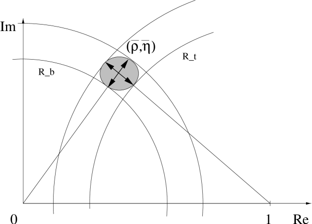
Figure 4: Unitarity “triangle”, assuming the SM range for $\gamma$.

The $g_{i}$ are of order $\frac{v^{2}}{\Lambda^{2}}$ which translates into a limit of roughly $\Lambda\geq 500\,{\rm GeV}$

5 Implications for neutral currents

Finally we have to consider the effect on neutral currents, in particular on flavour changing neutral currents (FCNCs). The tree-level contributions to FCNCs are absent by construction, but through loops the charged currents induce modifications of the neutral currents. The insertion of the effective CKM matrix for the charged currents induces a violation of the GIM mechanism which leads to FCNCs already at one loop.

The obvious example for such an effect is an effective left-handed FCNC coupling to the $Z$ boson induced by the loop diagrams shown in fig. 5. They lead to a mixing of the operators $O_{LL}$ such that off-diagonal contributions to $O^{(2)}_{LL}$ and the neutral components of $O^{(1)}_{LL}$ appear. These contributions are expected to be small, although they are enhanced by a large logarithm of the type $\ln(\Lambda/M_{W})$ where $\Lambda$ is the scale of new physics. The suppression originates on the one hand from the electroweak loop factor $g^{2}/(16\pi^{2})$ and on the other hand from the fact that this contribution is proportional to the GIM violation (290, 291), which has to be a small quantity as well.

HMZoneloop (50,20) thick a0,a1,i,a2 b0,b1,o,b2 z fermion,label=$d$,label.side=lefti,v1 phantom,tension=2v1,v2,v3 fermion,label=$d^{\prime}$,label.side=leftv3,o decor.shape=square,decor.size=5thick,decor.filled=30v1 v3 boson,label=$W$,label.side=right,leftv1,v3 boson,label=$Z$,label.side=leftv2,z fermionv1,v2,v3   (50,20) thick a0,a1,i,a2 b0,b1,o,b2 z fermion,label=$d$,label.side=lefti,v1 phantom,tension=2v1,v2,v3 fermion,label=$d^{\prime}$,label.side=leftv3,o decor.shape=square,decor.size=5thick,decor.filled=30v1 v3 fermionv1,v3 boson,label=$W$,label.side=left,right,tag=1v1,v3 phantom,tag=2v2,z p[] p1vpath1(__v1, __v3) p2vpath2(__v2, __z) boson,label=$Z$,label.side=leftpoint length(p1)/2 of p1 – point length(p2) of p2 decor.shape=circle,decor.filled=full,decor.size=2thickpoint length(p1)/2 of p1

Figure 5: Diagrams leading to FCNCs on the one-loop level. This corresponds to a mixing of the Operators $O_{LL}$.

Another effect of similar type is the modification of the $\rho$ parameter, whose deviation from unity is defined as usual by

$$\Delta\rho=\frac{A_{ZZ}(0)}{M_{Z}^{2}}-\frac{A_{WW}(0)}{M_{W}^{2}}$$ (316)

where $A_{ZZ}$ and $A_{WW}$ are the transverse contributions to the $Z$ and the $W$ self energies.

Clearly there is a contribution to the $\rho$ parameter from dimension-six operators which contain only Higgs and gauge fields [3]. An example is the operator

$$R={\rm Tr}\left\{L_{\mu}L_{3}^{\mu}\right\}$$ (317)

which leads at tree level to a modification of $\rho$.

However, in our case we can consider the contribution of (223) and (232) to the $\rho$ parameter by computing the diagrams shown in fig. 6.

HMrhofigure (50,20) thick i o boson,label=$Z$,label.side=left,tension=2i,v1 boson,label=$Z$,label.side=left,tension=2v2,o fermion,left,label=$t$,label.side=leftv1,v2 fermion,left,label=$t$,label.side=leftv2,v1 decor.shape=square,decor.size=5thick,decor.filled=30v1 v2   and   (50,20) thick i o boson,label=$W$,label.side=left,tension=2i,v1 boson,label=$W$,label.side=left,tension=2v2,o fermion,left,label=$t$,label.side=leftv1,v2 fermion,left,label=$d,,s,,b$,label.side=leftv2,v1 decor.shape=square,decor.size=5thick,decor.filled=30v1 v2

Figure 6: One-loop diagrams for the new-physics contribution to the $\rho$ parameter. The box indicates the insertion of a vertex corresponding to $O_{LL}^{(1)}$ and $O_{LL}^{(2)}$.

In the standard model the $\rho$ parameter is convergent due to the fact that the divergencies of the charged and the neutral current cancel exactly. Including the new-physics contributions disturbs this cancellation, leading to an enhancement by a logarithm of the scale of the new-physics contribution. This indicates that a mixing of the operators (223) and (232) into operators of the type (317) occurs.

Keeping only the dominant contribution from the top quark we obtain

$$\Delta\rho=\frac{3G_{F}m_{t}^{2}}{2\pi^{2}\sqrt{2}}\left(-2g_{0}-g_{2}^{(u)}+g_{1}^{(d)}|V_{td}|^{2}+g_{2}^{(d)}|V_{tb}|^{2}\right)\ln\left(\frac{\Lambda^{2}}{M_{W}^{2}}\right).$$ (318)

We note that the operator (223) conserves the custodial $SU(2)_{C}$, while (232) breaks this symmetry. The contribution of (232) is proportional to the difference $v^{2}/\Lambda^{2}\left(G_{u}-G_{d}\right)=2g_{0}\mathbbm{1}$, while the $SU(2)_{C}$ conserving piece is $v^{2}/\Lambda^{2}\left(G_{u}+G_{d}\right)=\Delta g\mathbbm{1}$. The $\rho$-parameter is a measure of $SU(2)_{C}$ breaking and hence it cannot depend on $\Delta g$. Although the case $v^{2}/\Lambda^{2}\,G_{u}=-v^{2}/\Lambda^{2}\,G_{d}=g_{0}\mathbbm{1}$ corresponds to the case where the CKM matrix is unitary despite a possible new-physics contribution, it still changes the strength of the charged current relative to the neutral one, and thus this appears in the $\rho$ parameter. In turn $v^{2}/\Lambda^{2}\left(G_{u}+G_{d}\right)=\Delta g\mathbbm{1}$ changes both the coupling of the neutral as well as the charged currents by the same amount, but this has to lead to a non-unitary CKM matrix with $V_{\textit{\scriptsize{eff}}}V_{\textit{\scriptsize{eff}}}^{\dagger}=(1+\Delta g)\mathbbm{1}$.

Likewise, the remaining terms in (318) have a similarly simple explanation. Already the mass matrices of the standard model violate $SU(2)_{C}$ leading to nontrivial mixings. If this effect was absent, we would have $V_{td}=0$ and $V_{tb}=1$. If now the new physics effects would conserve $SU(2)_{C}$ we would have $g_{2}^{(u)}=-g_{2}^{(d)}$ in which case the $\rho$ parameter again would not be affected.

Finally we may also consider the effect of the new-physics contributions in (223) and (232) on the forward-backward asymmetry for bottom quarks produced in $e^{+}e^{-}$ collisions on the $Z$ resonance. On resonance the forward-backward asymmetry is given by

$$A_{FB}=\frac{3}{4}\left(\frac{g_{L,e}^{2}-g_{R,e}^{2}}{g_{L,e}^{2}+g_{R,e}^{2}}\right)\left(\frac{g_{L,b}^{2}-g_{R,b}^{2}}{g_{L,b}^{2}+g_{R,b}^{2}}\right)$$ (319)

where $g_{L,i}$ and $g_{R,i}$ are the left- and right-handed couplings of the particle $i$.

According to (223) and (232) we assume that only the left-handed couplings of the bottom quark deviate from the standard model values. Inserting the couplings of the electron and the bottom quark we get

$$A_{FB} = \frac{9(4s_{W}^{2}-3)(4s_{W}^{2}-1)}{4(8s_{W}^{4}-12s_{W}^{2}+9)(8s_{W}^{4}-4s_{W}^{2}+1)}$$

$$\quad-\frac{36s_{W}^{4}(2s_{W}^{2}-3)(4s_{W}^{2}-1)}{(8s_{W}^{4}-12s_{W}^{2}+9)^{2}(8s_{W}^{4}-4s_{W}^{2}+1)}\,g_{b}$$

where $s_{W}^{2}=\sin^{2}\Theta_{W}$ is the weak mixing parameter and $g_{b}$ is of order $v^{2}/\Lambda^{2}$.

It is interesting to note that the coefficient in front of the new-physics parameter $g_{b}$ is very small; putting in $s_{W}^{2}\approx 0.2314$ which reproduces the best fit for the SM [12] one obtains

$$A_{FB}=0.1039-0.016g_{b}$$ (321)

which makes such an effect hard to observe. Currently there is a statistically insignificant deviation of the measured value $A_{FB}=0.0994\pm 0.0017$ from the standard model expectation. Attributing this to $g_{b}$ yields $g_{b}\sim 0.3$ which is quite enormous, because $g_{b}$ is of order $v^{2}/\Lambda^{2}$ and such a value would lead to a relatively low $\Lambda$ of order 500 GeV.

6 Conclusions

We suggest a possible parametrisation of new-physics effects in flavour physics. It is based on considerations of dimension-six operators, out of which we have discussed the operators with two quark fields only. Making two more assumptions which is flavour conservation and the existence of a massless limit we can reduce the number of new-physics parameters to six.

We discussed the impact of these contributions on charged as well as on neutral currents. In the sector of charged currents, our parametrisation affects the analysis of the $B$ physics unitarity triangle in a well defined way by replacing the CKM matrix by an effective one. However, with present data most of the parameters cannot be constrained significantly. Due to the fact that the effective CKM matrix is not necessarily unitary anymore flavour changing neutral currents receive contributions at one loop from the violation of the GIM mechanism which we assume to be small. Furthermore, in the neutral currents the $SU(2)_{C}$ violating parameters affect the $\rho$ parameter yielding a possible contribution of order $M_{W}^{2}/\Lambda^{2}\ln(\Lambda^{2}/M_{W}^{2})$; however, the neutral currents test a different set of parameters as the CKM analysis. Finally, the forward backward asymmetry in $e^{+}e^{-}\to Z_{0}\to\bar{b}b$ is not very sensitive due to a small coefficient.

Clearly the analysis of the above set of operators cannot cover the full variety of possible new-physics contributions in the flavour sector. In particular, the set of all possible four-fermion operators has a nontrivial flavour structure, but is very large. Consequently one has to impose additional assumptions concerning these operators to deal with them in practical applications.

One possibility, which has been discussed already in [1], is to impose additional symmetries such as a horizontal or family symmetry. However, in general the couplings of the charged and neutral currents turn out to be of similar size. Using the stringent constraints on FCNCs yields very small couplings for the neutral current operators, which in turn then implies that also the charged current contributions will have very small couplings. At least in scenarios of this type it is justified to neglect the four-fermion operators e.g. in the analysis of the $B$ physics unitarity triangle discussed above.

References

• [1] W. Buchmuller and D. Wyler, Nucl. Phys. B 268, 621 (1986).
• [2] M. E. Peskin and T. Takeuchi, Phys. Rev. D 46 (1992) 381.
• [3] H. Georgi, Nucl. Phys. B 363 (1991) 301.
• [4] G. Buchalla, G. Hiller and G. Isidori, Phys. Rev. D 63, 014015 (2001) [arXiv:hep-ph/0006136].
• [5] G. D’Ambrosio, G. F. Giudice, G. Isidori and A. Strumia, Nucl. Phys. B 645 (2002) 155 [arXiv:hep-ph/0207036].
• [6] V. Barger, T. Han, P. Langacker, B. McElrath and P. Zerwas, arXiv:hep-ph/0301097.
• [7] D. Espriu and J. Manzano, Phys. Rev. D 63 (2001) 073008 [arXiv:hep-ph/0011036].
• [8] S. L. Glashow, J. Iliopoulos and L. Maiani, Phys. Rev. D 2 (1970) 1285.
• [9] K. Hagiwara et al. [Particle Data Group Collaboration], Phys. Rev. D 66 (2002) 010001.
• [10] Y. Grossman, Y. Nir and M. P. Worah, Phys. Lett. B 407, 307 (1997) [arXiv:hep-ph/9704287].
• [11] A. Hocker, H. Lacker, S. Laplace and F. Le Diberder, Eur. Phys. J. C 21 (2001) 225 [arXiv:hep-ph/0104062].
• [12] P. B. Renton, Rept. Prog. Phys.  65 (2002) 1271 [arXiv:hep-ph/0206231].