$B^{0}-\bar{B}^{0}$ mixing beyond factorization

Abstract

We present a calculation of the $B^{0}-\bar{B}^{0}$ mixing matrix element in the framework of QCD sum rules for three-point functions. We compute $\alpha_{s}$ corrections to a three-point function at the three-loop level in QCD perturbation theory, which allows one to extract the matrix element with next-to-leading order (NLO) accuracy. This calculation is imperative for a consistent evaluation of experimentally-measured mixing parameters since the coefficient functions of the effective Hamiltonian for $B^{0}-\bar{B}^{0}$ mixing are known at NLO. We find that radiative corrections violate factorization at NLO; this violation is under full control and amounts to 10%.

The phenomenon of particle-antiparticle mixing, possible in systems of neutral mesons of different flavors, is the primary source of studies of CP violation (for review, see e.g. buhalla ). According to the Cabibbo-Kobayashi-Maskawa (CKM) picture, quarks of all three generations must be present in a transition for CP violation to occur. Historically, studies of $K^{0}-\bar{K}^{0}$ mixing provided first essential insights into the physics of heavy particles as well as tests of general concepts of quantum field theory. For a long time it was the only place where the effects of CP violation were clearly established (see e.g. kkreviewOLD ). Since weak couplings of $s$ and $d$ quarks to third generation quarks are small, experimental studies of CP violation in heavy mesons are considered more promising. While recent experimental results for heavy charmed mesons $D(\bar{u}c)$ are encouraging, a full consistent theoretical description of this system is still lacking Petrov:2002is . These considerations make the systems of $B_{d}(\bar{d}b)$ and $B_{s}(\bar{s}b)$ mesons the most promising laboratory for a precision analysis of CP violation and mixing both experimentally and theoretically reviewBB . Hereafter we shall consider $B_{d}$ mesons. The generalization to $B_{s}$ mesons is straightforward.

Phenomenologically the system of the $B^{0}-\bar{B}^{0}$ mesons is described by the effective mass operator $\left(M-i\Gamma/2\right)_{ij}$, $\{i,j\}=\{1,2\}$ which in the presence of $\Delta B=2$ interactions acquires non-diagonal terms. The difference between the values of the mass eigenstates of $B$ mesons $\Delta m=M_{heavy}-M_{light}\approx 2\left|M_{12}\right|$ is an important observable which is precisely measured to be $\Delta m=0.489\pm 0.005(stat)\pm 0.007(syst)~{}ps^{-1}$ PDG . With an adequate theoretical description, it can be used to extract top quark CKM parameters.

In the standard model, the effective low-energy Hamiltonian describing $\Delta B=2$ transitions has been computed at next-to-leading order (NLO) in QCD perturbation theory (PT) Buras

$$H_{\mbox{eff}}^{\triangle B=2} = \frac{G_{F}^{2}M_{W}^{2}}{4\pi^{2}}\left({V_{tb}}^{*}V_{td}\right)^{2}\eta_{B}S_{0}(x_{t})$$

$$\times \left[\alpha_{s}^{(5)}(\mu)\right]^{-6/23}\left[1+\frac{\alpha_{s}^{(5)}(\mu)}{4\pi}J_{5}\right]{\cal O}(\mu)$$

where $\eta_{B}=0.55\pm 0.1$ Buras:1990fn , $J_{5}=1.627$ in the naive dimensional regularization (NDR) scheme, $S_{0}(x_{t})$ is the Inami-Lim function Inami:1980fz , and ${\cal O}(\mu)=(\bar{b}_{L}\gamma_{\sigma}d_{L})(\bar{b}_{L}\gamma_{\sigma}d_{L})(\mu)$ is a local four-quark operator at the normalization point $\mu$. Note that the part of Eq. ($B^{0}-\bar{B}^{0}$ mixing beyond factorization) in the second line is renormalization-group (RG) invariant. Mass splitting of heavy and light mass eigenstates can then be found to be

$$\Delta m=2|\langle\bar{B}^{0}|H_{\mbox{eff}}^{\triangle B=2}|B^{0}\rangle|$$ (2)

$$=~{}\!\!{\cal C}\left[\alpha_{s}^{(5)}(\mu)\right]^{-6/23}\left[1+\frac{\alpha_{s}^{(5)}(\mu)}{4\pi}J_{5}\right]\langle\bar{B}^{0}|{\cal O}(\mu)|B^{0}\rangle$$

where ${\cal C}=G_{F}^{2}M_{W}^{2}\left({V_{tb}}^{*}V_{td}\right)^{2}\eta_{B}m_{B}S_{0}(x_{t})/\left(4\pi^{2}\right)$. The largest uncertainty of about 30% in the theoretical calculation is introduced by the poorly known hadronic matrix element ${\cal A}=\langle\bar{B}^{0}|{\cal O}(\mu)|B^{0}\rangle$ PDG . The evaluation of this matrix element is a genuine non-perturbative task, which can be approached with several different techniques. The simplest approach (“factorization”) Gaillard:1974hs reduces the matrix element ${\cal A}$ to the product of matrix elements measured in leptonic $B$ decays ${\cal A}^{f}=(8/3)$ $\langle\bar{B}^{0}|\bar{b}_{L}\gamma_{\sigma}d_{L}|0\rangle\langle 0|\bar{b}_{L}\gamma^{\sigma}d_{L}|B^{0}\rangle=(2/3)f_{B}^{2}m_{B}^{2}$ where the decay constant $f_{B}$ is defined by $\langle 0|\bar{b}_{L}\gamma_{\mu}d_{L}|B^{0}({\bf p})\rangle=ip_{\mu}f_{B}/2$. A deviation from the factorization ansatz is usually described by the parameter $B_{B}$ defined as ${\cal A}=B_{B}{\cal A}^{f}$; in factorization $B_{B}=1$. There are many approaches to evaluate this parameter (and the analogous parameter $B_{K}$ of $K^{0}-\bar{K}^{0}$ mixing) available in the literature Bardeen ; ope-three-kk ; bb-three ; Reinders ; Narison ; Melikhov ; lattice ; Hiorth .

The calculation of the hadronic mixing matrix elements using Operator Product Expansion (OPE) and QCD sum rule techniques for three-point functions ope-three-kk ; bb-three ; Reinders is very close in spirit to lattice computations lattice , which is a model-independent, first-principles method. In the QCD sum rule approach one relies on asymptotic expansions of a Green’s function while on the lattice the function itself can be computed in principle. The sum rule techniques also provide a consistent way of taking into account perturbative corrections to matrix elements which is needed to restore the RG invariance of physical observables usually violated in the factorization approximation kkaplhas . The calculation of perturbative corrections to $B^{0}-\bar{B}^{0}$ mixing using OPE and sum rule techniques is the main subject of this paper. A concrete realization of the sum rule method applied here consists of the calculation of the moments of the three-point correlation function of the interpolating operators of the $B$-meson and the local operator ${\cal O}(\mu)$ responsible for $B^{0}-\bar{B}^{0}$ transitions.

Let us consider the three-point correlation function

$$\Pi(p_{1},p_{2})=\int dxdy\langle 0|TJ_{\bar{B}}(x){\cal O}(0)\bar{J}_{B}(y)|0\rangle e^{ip_{2}x-ip_{1}y}.$$

The operator $J_{B}=(m_{b}+m_{d})\bar{d}i\gamma_{5}b$ is chosen as interpolating current for the $B^{0}$-meson and $m_{b}$ is the $b$ quark mass. Note that $J_{B}$ is RG invariant, $J_{B}=\partial_{\mu}(\bar{d}\gamma_{\mu}\gamma_{5}b)$ and $\langle 0|J_{B}(0)|B^{0}(p)\rangle=f_{B}m_{B}^{2}$ where $m_{B}$ is the $B$-meson mass. A dispersive representation of the correlator reads

$$\Pi(p_{1},p_{2})\equiv\Pi(p_{1}^{2},p_{2}^{2},q^{2})=\int\frac{\rho(s_{1},s_{2},q^{2})ds_{1}ds_{2}}{(s_{1}-p_{1}^{2})(s_{2}-p_{2}^{2})}$$ (3)

where $q=p_{2}-p_{1}$. For the analysis of $B^{0}-\bar{B}^{0}$ mixing this correlator needs to be computed at $q=0$, while within the sum rule framework $q^{2}=0$. This particular kinematical point is infrared safe for massive quarks.

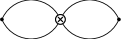
Figure 1: Perturbation theory diagram at LO

The matrix element $\langle\bar{B}^{0}|{\cal O}(\mu)|B^{0}\rangle$ appears in the three-point correlator as a contribution of the $B$-mesons in the form of a double pole

$$\Pi(p_{1}^{2},p_{2}^{2},q^{2})=\frac{\langle J_{\bar{B}}|\bar{B}^{0}\rangle}{m_{B}^{2}-p_{1}^{2}}\langle\bar{B}^{0}|{\cal O}(\mu)|B^{0}\rangle\frac{\langle B^{0}|\bar{J}_{B}\rangle}{m_{B}^{2}-p_{2}^{2}}+\ldots$$ (4)

where the ellipsis stand for higher resonances and continuum contributions. The matrix element can be extracted by comparing the representations given in Eq. (4) and the (smeared) theoretical expression of Eq. (3) obtained with an asymptotic expansion based on OPE. Note that the analytical calculation of the spectral density itself at NLO of PT expansion is beyond present computational techniques. Therefore, a practical way of extracting the $B^{0}-\bar{B}^{0}$ matrix element is to analyze the moments of the correlation function at ${p_{1}^{2}=p_{2}^{2}=0}$ at the point $q^{2}=0$. One obtains

$$M(i,j)\equiv\frac{\partial^{i+j}\Pi(p_{1}^{2},p_{2}^{2},0)}{i!j!\partial p_{1}^{2i}\partial p_{2}^{2j}}=\int\frac{\rho(s_{1},s_{2},0)ds_{1}ds_{2}}{s_{1}^{i+1}s_{2}^{j+1}}\,.$$

A theoretical computation of these moments reduces to an evaluation of single scale vacuum diagrams (we neglect the light quark masses). This calculation can be done analytically with available tools for the automatic computation of multi-loop diagrams.

The leading contribution to the asymptotic expansion is given by the diagram shown in Fig. 1. At leading order (LO) in QCD perturbation theory the three-point function of Eq. ($B^{0}-\bar{B}^{0}$ mixing beyond factorization) completely factorizes $\Pi(p_{1},p_{2})=(8/3)$$\Pi_{\mu}(p_{1})\Pi^{\mu}(p_{2})$ where $\Pi_{\mu}(p)$ is the two-point correlator

$$\Pi_{\mu}(p)=p_{\mu}\Pi(p^{2})=\int dxe^{ipx}\langle 0|TJ_{\bar{B}}(x)\bar{b}_{L}\gamma_{\mu}d_{L}(0)|0\rangle.$$ (5)

The calculation of moments is straightforward since the double spectral density $\rho(s_{1},s_{2},q^{2})$ can be explicitly found. Using a dispersive representation of $\Pi(p^{2})$

$$\Pi(p^{2})=\int_{m^{2}}^{\infty}\frac{\rho(s)ds}{s-p^{2}},\quad\rho(s)=\frac{3}{16\pi^{2}}m^{2}\left(1-\frac{m^{2}}{s}\right)^{2}$$ (6)

one finds the LO double spectral density $\rho^{\rm LO}(s_{1},s_{2},q^{2})=(8/3)(p_{1}\cdot p_{2})\rho(s_{1})\rho(s_{2})=(4/3)(s_{1}+s_{2}-q^{2})\rho(s_{1})\rho(s_{2})$. First non-factorizable contributions to Eq. (3) appear at NLO. Nevertheless, the factorizable diagrams form an important subset of all contributions, as they are independently gauge and RG invariant. Thus, a classification of diagrams in terms of their factorizability is a very powerful technique in the quantitative analysis.

The NLO factorizable contributions are given by the product of two-point correlation functions from Eq. (5), as shown in Fig. 2.

Figure 2: Factorizable diagrams at NLO

Writing $\Pi(p^{2})=\Pi_{\rm LO}(p^{2})+\Pi_{\rm NLO}(p^{2})$ we obtain $\Pi_{\rm NLO}^{f}(p_{1},p_{2})$$=$$(8/3)$$(p_{1}.p_{2})$$(\Pi_{\rm LO}(p_{1}^{2})\Pi_{\rm NLO}(p_{2}^{2})$ $+$$\Pi_{\rm NLO}(p_{1}^{2})\Pi_{\rm LO}(p_{2}^{2}))$. The spectral density of the correlator $\Pi_{\rm NLO}(p^{2})$ is known analytically. This completely solves the problem of the NLO analysis in factorization. Note that even a NNLO analysis of factorizable diagrams is possible as several moments of two-point correlators are known analytically. Others can be obtained numerically from the approximate spectral density chetmomnondiag .

The NLO analysis of non-factorizable contributions within perturbation theory is the main result of this paper. This analysis amounts to the calculation of a set of three-loop diagrams (a typical diagram is presented in Fig. 3). These diagrams can be computed using the package MATAD for automatic calculation of Feynman diagrams matad . Before applying this package, the combinatorics of disentangling the tensorial structures has to be solved and all the diagrams have to be reduced to a set of scalar integrals which can be done using the results of ref. Davyd . The steps described above were automized with the computer algebra system FORM form . We shall present the details of this calculation elsewhere.

The local four-quark operator ${\cal O}$ entering the effective Hamiltonian has to be renormalized. We employ dimensional regularization with an anticommuting $\gamma_{5}$.

Figure 3: An example of a non-factorizable diagram at NLO

The renormalization of the operator ${\cal O}$ reads

$${\cal O}^{R}={\cal O}^{B}-\frac{\alpha_{s}}{4\pi}\frac{1}{\varepsilon}{\cal O}_{c}$$ (7)

with ${\cal O}_{c}=(\bar{b}_{L}\Gamma_{\mu\nu\alpha}t^{a}d_{L})(\bar{b}_{L}\Gamma^{\mu\nu\alpha}t^{a}d_{L})$. The $t^{a}$ are the $SU_{c}(3)$ generators and $\Gamma_{\mu\nu\alpha}$$=(\gamma_{\mu}\gamma_{\nu}\gamma_{\alpha}$$-\gamma_{\alpha}\gamma_{\nu}\gamma_{\mu})/2$. The renormalization of the factorizable contributions reduces to that of the $b$-quark mass $m$. We use the quark pole mass as a mass parameter of the calculation.

The expression for the “theoretical” moments reads

$$M_{th}(i,j)=\frac{m^{6}a_{ij}}{m^{2(i+j)}}\left(1+\frac{\alpha_{s}}{4\pi}\left(b^{f}_{ij}+b^{nf}_{ij}\right)\right)$$ (8)

where the quantities $a_{ij}$, $b^{f}_{ij}$ and $b^{nf}_{ij}$ represent LO, NLO factorizable and NLO nonfactorizable contributions as shown in Figs. 1-3. The NLO nonfactorizable contributions $b^{nf}_{ij}$ with $i+j\leq 7$ are analytically calculated in this paper for the first time. The calculation required about 24 hours of computing time on a dual-CPU 2 GHz Intel Xeon machine. The calculation of higher moments is feasible but requires considerable optimization of the code. This work is in progress and will be presented elsewhere. As an example, we give the analytical results for the lowest finite moment $M_{th}(2,2)$:

$$a_{22}=\frac{1}{(16\pi^{2})^{2}}\left(\frac{8}{3}\right),\quad b^{f}_{22}=\frac{40}{3}+\frac{16\pi^{2}}{9}\,,$$ (9)

$$b^{nf}_{22}=S_{2}\frac{8366187}{17500}-\zeta_{3}\frac{84608}{875}-\pi^{2}\frac{33197}{52500}-\frac{426319}{315000}.$$

Here $S_{2}=\frac{4}{9\sqrt{3}}{\rm Cl}_{2}\left(\frac{\pi}{3}\right)=0.2604\ldots$, $\zeta_{3}=\zeta(3)$, and $\mu^{2}=m^{2}$. For higher moments we present only numerical values for $b^{nf}_{ij}$: $b^{nf}_{2(2345)}=\{0.68,1.22,1.44,1.56\}$ and $b^{nf}_{3(34)}=\{1.96,2.25\}$. The nonperturbative contribution due to the gluon condensate is small. For the standard numerical value $\langle g^{2}_{s}G^{2}\rangle=0.5~{}{\rm GeV}^{4}$ svz , the nonfactorizable contribution due to the gluon condensate amounts to about 3% of the perturbative contribution for the high moment $M(3,3)$. For lower moments it is even smaller and, therefore, can be safely neglected in the whole analysis.

We use the above theoretical results to analyze sum rules and extract the non-perturbative parameter $B_{B}$.

The “phenomenological” side of the sum rules is given by the moments which can be inferred from Eq. (4)

$$M_{ph}(i,j)=\frac{8}{3}B_{B}\frac{f_{B}^{4}m_{B}^{2}}{m_{B}^{2(i+j)}}$$ (10)

$$+{\cal O}\left(\frac{1}{(m_{B}^{2}+\Delta)^{i+1}m_{B}^{2j}},\frac{1}{(m_{B}^{2}+\Delta)^{j+1}m_{B}^{2i}}\right)$$

where the contribution of the $B$-meson is displayed explicitly. The remaining parts are the contributions due to higher resonances and the continuum which are suppressed due to the mass gap $\Delta$ in the spectrum model.

For comparison we consider the factorizable approximation for both “theoretical”

$$M_{th}^{f}(i,j)=\frac{m^{6}a_{ij}}{m^{2(i+j)}}\left(1+\frac{\alpha_{s}}{4\pi}b^{f}_{ij}\right)$$ (11)

and “phenomenological” moments, which, by construction, are built from the moments of the two-point function of Eq. (5)

$$M_{ph}^{f}(i,j)=\frac{8}{3}\frac{f_{B}^{4}m_{B}^{2}}{m_{B}^{2(i+j)}}+...$$ (12)

According to standard QCD sum rule technique, the “theoretical” calculation is dual to the “phenomenological” one. Thus, Eq. (10) should be equivalent (in the sum rule sense) to Eq. (8). Also, in factorization, Eq. (12) is equivalent to Eq. (11). Now Eq. (11) and Eq. (8) differ only due to non-factorizable corrections. Therefore, the difference between Eq. (12) and Eq. (10) is because the residues differ from their factorized values.

To find the nonfactorizable addition to $B_{B}$ from the sum rules we form ratios of the total and factorizable contributions. On the “theoretical” side one finds

$$\frac{M_{th}(i,j)}{M_{th}^{f}(i,j)}=1+\frac{\alpha_{s}}{4\pi}\frac{b^{nf}_{ij}}{1+\frac{\alpha_{s}}{4\pi}b^{f}_{ij}}\,.$$ (13)

This ratio is mass-independent. On the “phenomenological” side we have

$$\frac{M_{ph}(i,j)}{M_{ph}^{f}(i,j)}=\frac{B_{B}+R_{B}(z^{j}+z^{i})+C_{B}z^{i+j}}{1+R^{f}(z^{j}+z^{i})+C^{f}z^{i+j}}$$ (14)

where $z=m_{B}^{2}/(m_{B}^{2}+\Delta)$ is a parameter that describes the suppression of higher state contributions. $\Delta$ is a gap between the squared masses of the $B$-meson and higher states. $R_{B}$, $C_{B}$, $R^{f}$ and $C^{f}$ are parameters of the model for higher state contributions within the sum rule approach. In order to extract the non-factorizable contribution to $B_{B}$ we write $B_{B}=1+\Delta B$. Similarly, one can parameterize contributions to “phenomenological” moments due to higher $B$-meson states by writing $R_{B}=R^{f}+\Delta R$ and $C_{B}=C^{f}+\Delta C$. Clearly, $\Delta B=\Delta R=\Delta C=0$ in factorization. We obtain

$$\frac{M_{ph}(i,j)}{M_{ph}^{f}(i,j)}=1+\frac{\Delta B+\Delta R(z^{j}+z^{i})+\Delta Cz^{i+j}}{1+R^{f}(z^{j}+z^{i})+C^{f}z^{i+j}}\,.$$ (15)

Comparing Eqs. (13) and (15) one sees how the perturbative non-factorizable correction $b^{nf}_{ij}$ is “distributed” among the phenomenological parameters of the spectrum. We extract $\Delta B$ by a combined fit of several “theoretical” and “phenomenological” moments. The final formula for the determination of $\Delta B$ reads

$$\frac{\alpha_{s}}{4\pi}b^{nf}_{ij}=\Delta B+\Delta R(z^{j-2}+z^{i-2})+\Delta Cz^{i+j-4}$$ (16)

where $\Delta R$ and $\Delta C$ are free parameters of the fit. We take $\Delta=0.4m_{B}^{2}$ which corresponds to the duality interval of $1~{}{\rm GeV}$ in energy scale within the HQET analysis of the $B$ meson two-point correlator. We then perform least-squares fit to determine $\Delta B$. Using all available theoretical moments we find $(\Delta B,\Delta R,\Delta C)$$=\alpha_{s}(m)/(4\pi)$$(7.1,-5.0,3.6)$. We checked the stability of the sum rules which lead to a prediction of $\Delta B$. It can be illustrated in the following way. The contribution of higher $B$ states is suppressed more strongly for higher moments and therefore decreases with increasing order of a moment, while the perturbative correction grows. The sum of both is (approximately) the same for all moments, which leads to a (almost) constant value for $\Delta B$, independent of the particular moment. The calculation can be further improved with the evaluation of higher moments. The result is sensitive to the parameter $z$ or to the magnitude of the mass gap $\Delta$ used in the parametrization of the spectrum. Estimating all uncertainties we finally find the NLO non-factorizable QCD corrections to $\Delta B$ due to perturbative contributions to the sum rules to be $\Delta B=(6\pm 1)\alpha_{s}(m)/(4\pi)$. For $m=4.8~{}{\rm GeV}$, $\alpha_{s}(m)=0.2$ PDG ; Penin:1999kx it leads to $\Delta B=0.095\approx 0.1$. It is known that nonperturbative corrections (such as the ones due to the quark-gluon condensate) to the parameter $B_{B}$ are negative, $\Delta B^{nonPT}(m)=-0.05$ bb-three . Combining this result with the present analysis we find $B_{B}(m)=1+0.1_{PT}-0.05_{nonPT}$ showing the excellent numerical validity of the factorization approximation at the scale $\mu=m$.

In conclusion, we have evaluated the $B^{0}-\bar{B}^{0}$ mixing matrix element in the framework of QCD sum rules for three-point functions at NLO in perturbative QCD. The effect of radiative corrections on $B_{B}$ is under complete control and amounts to approximately $+10$%. We have also shown that perturbative QCD correction to $\Delta B$ for the moments considered in our analysis completely dominates the correction due to the gluon condensate.

We thank Rob Harr for fruitful discussions. This work was supported in part by the Russian Fund for Basic Research under contracts 01-02-16171 and 02-01-00601, by Volkswagen grant No. I/77788, and by the US Department of Energy under grant DE-FG02-96ER41005.

References

- (1) G. Buchalla, A. J. Buras and M. Lautenbacher, Rev. Mod. Phys. 68, 1125 (1996).
- (2) I. I. Bigi and A. I. Sanda, Cambridge Monogr. Part. Phys. Nucl. Phys. Cosmol. 9, 1 (2000).
- (3) A. A. Petrov, arXiv:hep-ph/0207212.
- (4) A. Ali and D. London, arXiv:hep-ph/0002167.
- (5) K. Hagiwara et al., Phys. Rev. D 66, 010001 (2002).
- (6) F. J. Gilman and M. B. Wise, Phys. Rev. D 27, 1128 (1983); A. J. Buras, arXiv:hep-ph/9806471.
- (7) A. J. Buras, M. Jamin and P. H. Weisz, Nucl. Phys. B 347, 491 (1990); J. Urban, F. Krauss, U. Jentschura and G. Soff, Nucl. Phys. B 523, 40 (1998).
- (8) T. Inami and C. S. Lim, Prog. Theor. Phys. 65, 297 (1981) [Erratum-ibid. 65, 1772 (1981)].
- (9) M. Gaillard and B. Lee, Phys. Rev. D 10, 897 (1974).
- (10) J. Bijnens, H. Sonoda and M. B. Wise, Phys. Rev. Lett. 53, 2367 (1984); W. A. Bardeen, A. J. Buras and J. M. Gerard, Phys. Lett. B 211, 343 (1988).
- (11) K. G. Chetyrkin et al., Phys. Lett. B 174, 104 (1986); L. J. Reinders and S. Yazaki, Nucl. Phys. B 288, 789 (1987);
- (12) A. A. Ovchinnikov and A. A. Pivovarov, Sov. J. Nucl. Phys. 48, 120 (1988); Phys. Lett. B 207, 333 (1988); A. A. Pivovarov, arXiv:hep-ph/9606482.
- (13) L. J. Reinders and S. Yazaki, Phys. Lett. B 212, 245 (1988).
- (14) A. Pich, Phys. Lett. B 206, 322 (1988); S. Narison and A. A. Pivovarov, Phys. Lett. B 327, 341 (1994).
- (15) D. Melikhov and N. Nikitin, Phys. Lett. B 494, 229 (2000).
- (16) D. Becirevic et al., Phys. Lett. B 487, 74 (2000); D. Becirevic et al., Nucl. Phys. B 618, 241 (2001); M. Lusignoli, G. Martinelli and A. Morelli, Phys. Lett. B 231, 147 (1989); M. Lusignoli, L. Maiani, G. Martinelli and L. Reina, Nucl. Phys. B 369, 139 (1992); C. T. Sachrajda, Nucl. Instrum. Meth. A 462, 23 (2001); J. M. Flynn and C. T. Sachrajda, Adv. Ser. Direct. High Energy Phys. 15, 402 (1998).
- (17) A. Hiorth and J. O. Eeg, Eur. Phys. J. C 30, 006 (2003).
- (18) A. A. Pivovarov, Int. J. Mod. Phys. A 10, 3125 (1995).
- (19) K. G. Chetyrkin, M. Steinhauser, arXiv:hep-ph/0108017.
- (20) M. Steinhauser, Comput. Phys. Commun. 134, 335 (2001).
- (21) A. I. Davydychev and J. B. Tausk, Nucl. Phys. B 465, 507 (1996).
- (22) J. A. Vermaseren, arXiv:math-ph/0010025.
- (23) M. A. Shifman, A. I. Vainshtein and V. I. Zakharov, Nucl. Phys. B 147, 448 (1979).
- (24) A. A. Penin and A. A. Pivovarov, Nucl. Phys. B 549, 217 (1999).