Remarks on heavy-quark production
in photon-nucleon and photon-photon collisions

Abstract

I discuss mechanisms of heavy quark production in (real) photon-nucleon and (real) photon - (real) photon collisions. In particular, I focuse on application of the Saturation Model. In addition to the main dipole-nucleon or dipole-dipole contribution included in recent analyses, I propose how to calculate within the same formalism the hadronic single-resolved contribution to heavy quark production. At high photon-photon energies this yields a sizeable correction of about 30-40 % for inclusive charm production and 15-20 % for bottom production. Adding all possible contributions to $e^{+}e^{-}\rightarrow b\bar{b}X$ together removes a huge deficit observed in earlier works but does not solve the problem totally.

1 Introduction

The total cross section for virtual photon - proton scattering in the region of small $x$ and intermediate $Q^{2}$ can be well described by the Saturation Model (SAT-MOD) [1]. The very good agreement with experimental data can be extended even to the region of rather small $Q^{2}$ by adjusting an effective quark mass. At present there is no deep understanding of the fit value of the parameter as we do not understand in detail the confinement and the underlying nonperturbative effects related to large size QCD contributions.

In this presentation I shall limit to the production of heavy quarks which is simpler and more transparent for real photons. Here one can partially avoid the problem of the poor understanding of the effective light quark mass, i.e. the domain of the large (transverse) size of the hadronic system emerging from the photon.

It was shown recently that the simple SAT-MOD description can be succesfully extended also to the photon-photon scattering [2]. The heavy quark production in photon-photon collisions is interesting in the context of a deficit of standard QCD predictions relative to the experimental data as observed recently for $b$ quark production.

2 Heavy quark production in photon-nucleon scattering

In the so-called dipole picture the cross section for heavy quark-antiquark ($Q\bar{Q}$) photoproduction on the nucleon can be written as

$$\sigma_{\gamma N\rightarrow Q\bar{Q}}(W)=\int d^{2}\rho dz\;|\Phi_{T}^{Q\bar{Q}}(\vec{\rho},z)|^{2}\sigma_{dN}(\rho,z,W)\;,$$ (1)

where $\Phi_{T}$ is (transverse) quark-antiquark photon wave function (see for instance [4]) and $\sigma_{dN}$ is the dipole-nucleon total cross section. Inspired by its phenomenological success [1] we shall use the SAT-MOD parametrization for $\sigma_{dN}$. Because for real photoproduction the Bjorken-$x$ is not defined we are forced to replace $x$ by $x_{g}$ [3].

In Fig.1a I show predictions of SAT-MOD for charm photoproduction. The dotted line represents calculations based on Eq.(1). The result of this calculation exceeds considerably the fixed target experimental data. One should remember, however, that the simple formula (1) applies at high energies only. At lower energies one should include effects due to kinematical threshold. In the momentum representation this can be done by requiring: $M_{Q\bar{Q}}<W$, where $M_{Q\bar{Q}}$ is the invariant mass of the final $Q\bar{Q}$ system. This upper limit still exceeds the low energy experimental data. There are phase space limitations in the region $x_{g}\rightarrow$ 1 which have been neglected so far. Those can be estimated using naive counting rules. Such a procedure leads to a reasonable agreement with the fixed target experimental data.

The deviation of the solid line from the dotted line gives an idea of the range of the safe applicability of SAT-MOD for the production of the charm quarks/antiquarks. The cross section for $W>$ 20 GeV is practically independent of the approximate treatment of the threshold effects. SAT-MOD seems to slightly underestimate the H1 collaboration data [5]. For comparison in Fig.1 we show the result of similar calculations in the collinear approach (thick dash-dotted line) with details described in [3].

The calculation above is not complete. For real photons a vector dominance contribution due to photon fluctuation into vector mesons should be included on the top of the dipole contribution. In the present calculation we include only the dominant gluon-gluon fusion component. Then

$$\sigma_{\gamma N\rightarrow Q\bar{Q}}^{VDM}(W)=\sum_{V}\frac{4\pi}{f_{V}^{2}}\;\int dx_{V}dx_{N}\;g_{V}(x_{V},\mu^{2}_{F})\;g_{N}(x_{N},\mu^{2}_{F})\;\sigma_{gg\rightarrow Q\bar{Q}}(\hat{W})\;.$$ (2)

Here the $f_{V}$ constants describe the transition of the photon into vector mesons ($\rho$, $\omega$, $\phi$). The gluon distributions in vector mesons are taken as that for the pion [7].

The dash-dotted line in Fig.1a shows the VDM contribution calculated in the leading order (LO) approximation for $\sigma_{gg\rightarrow Q\bar{Q}}$. The so-calculated VDM contribution is small at small energies but cannot be neglected at high energies.

The situation for bottom photoproduction seems similar. In Fig.1b I compare the SAT-MOD predictions with the data from the H1 collaboration [6]. Here the threshold effects survive up to very high energy $W\sim$ 50 GeV. Again the predictions of SAT-MOD are slightly below the H1 experimental data point. The relative magnitude of the VDM component is similar as for the charm production.

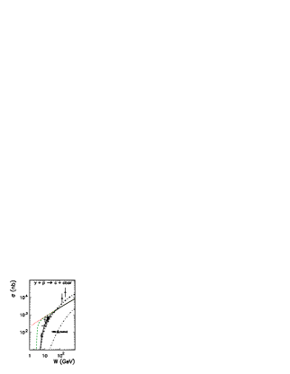
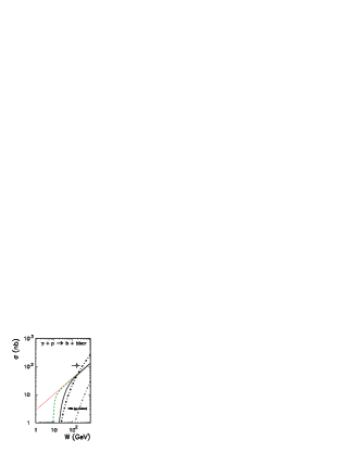
Figure 1: The cross section for $\gamma+p\rightarrow Q\bar{Q}X$. The dotted line: standard SAT-MOD, the dashed line: includes kinematical threshold, the solid line includes in addition a suppression by $(1-x_{c})^{7}$, the thick dash-dotted line: collinear approximation and the thin dash-dotted line: the LO VDM contribution.

3 Heavy quark production in photon-photon scattering

In the dipole-dipole approach the total cross section for $\gamma\gamma\rightarrow Q\bar{Q}$ production can be expressed as

$$\sigma_{\gamma\gamma\rightarrow Q\bar{Q}}^{dd}(W) = \sum_{f_{2}\neq Q}\int|\Phi^{Q\bar{Q}}(\rho_{1},z_{1})|^{2}|\Phi^{f_{2}\bar{f}_{2}}(\rho_{2},z_{2})|^{2}\sigma_{dd}(\rho_{1},\rho_{2},x_{Qf})\;d^{2}\rho_{1}dz_{1}d^{2}\rho_{2}dz_{2}$$

$$+ \sum_{f_{1}\neq Q}\int|\Phi^{f_{1}\bar{f}_{1}}(\rho_{1},z_{1})|^{2}|\Phi^{Q\bar{Q}}(\rho_{2},z_{2})|^{2}\sigma_{dd}(\rho_{1},\rho_{2},x_{fQ})\;d^{2}\rho_{1}dz_{1}d^{2}\rho_{2}dz_{2}\;,$$

where $\sigma_{dd}$ is the dipole-dipole cross section.

There are two problems associated with direct use of (LABEL:SM_QQbar). First of all, it is not completely clear how to generalize $\sigma_{dd}$ from $\sigma_{dN}$ parametrized in [1]. Secondly, formula (LABEL:SM_QQbar) is correct only at $W\gg 2m_{Q}$. At lower energies one should worry about proximity of the kinematical threshold.

In a very recent paper [2] a new phenomenological parametrization for $\sigma_{dd}$ has been proposed. The phenomenological threshold factor in [2] does not guarantee automatic vanishing of the cross section exactly below the true kinematical threshold $W=2m_{a}+2m_{b}$. Therefore, instead of the phenomenological factor I impose an extra kinematical constraint: $M_{f\bar{f}}+M_{Q\bar{Q}}<W$ on the integration in (LABEL:SM_QQbar).

It is also not completely clear how to generalize the energy dependence of $\sigma_{dN}$ in photon-nucleon scattering to the energy dependence of $\sigma_{dd}$ in photon-photon scattering. In [3] I have defined the parameter which controls the SAT-MOD energy dependence of $\sigma_{dd}$ in a symmetric way with respect to both photons. In comparison to the prescription in [2], our prescription leads to a small reduction of the cross section far from the threshold [3].

Up to now we have calculated the contribution when photons fluctuate into quark-antiquark pairs, which is not complete. The dipole approach must be supplemented by the resolved photon contribution. This contribution can be estimated in the vector dominance model when either of the photons fluctuates into vector mesons. If the first photon fluctuates into the vector mesons, the so-defined single-resolved contribution to the heavy quark-antiquark production can be calculated analogously to the photon-nucleon case as

$$\sigma^{SR,1}_{\gamma\gamma\rightarrow Q\bar{Q}}(W)=\sum_{V_{1}}\frac{4\pi}{f_{V_{1}}^{2}}\int|\Phi_{2}^{Q\bar{Q}}(\rho_{2},z_{2})|^{2}\sigma_{V_{1}d}(\rho_{2},x_{1})\;d^{2}\rho_{2}dz_{2}\;,$$ (4)

where $\sigma_{V_{1}d}$ is vector meson - dipole total cross section. In the spirit of SAT-MOD, we parametrize the latter exactly as for the photon-nucleon case [1] with a simple rescaling of the normalization factor $\sigma_{0}^{dV}=2/3\cdot\sigma_{0}^{dN}$. In the present calculation $\sigma_{0}^{dN}$ as well as the other parameters of SAT-MOD are taken from [1]. Analogously, if the second photon fluctuates into vector mesons we obtain

$$\sigma^{SR,2}_{\gamma\gamma\rightarrow Q\bar{Q}}(W)=\sum_{V_{2}}\frac{4\pi}{f_{V_{2}}^{2}}\int|\Phi_{1}^{Q\bar{Q}}(\rho_{1},z_{1})|^{2}\sigma_{dV_{2}}(\rho_{1},x_{2})\;d^{2}\rho_{1}dz_{1}\;.$$ (5)

This clearly doubles the first contribution (4) to the total cross section.

The integrations in (4) and (5) are not free of kinematical constraints. When calculating both single-resolved contributions, it should be checked additionally if the heavy quark-antiquark invariant mass $M_{Q\bar{Q}}$ is smaller than the total photon-photon energy $W$ (see [3]).

In Fig.2 I show different contributions to the inclusive $c/\bar{c}$ (left panel) and $b/\bar{b}$ (right panel) production in photon-photon scattering. The thick solid line represents the sum of all contributions.

Let us start from the discussion of the inclusive charm production. The experimental data of the L3 collaboration [9] are shown for comparison. The modifications discussed above lead to a small damping of the cross section in comparison to Ref.[2]. The corresponding result (long-dashed line) stays below the recent experimental data of the L3 collaboration [9]. The hadronic single-resolved contribution constitutes about 30 - 40 % of the main SM contribution. At high energies the cross section for the $2c2\bar{c}$ component is about 8 % of that for the single $c\bar{c}$ pair component. In the inclusive cross section its contribution should be doubled because each of the heavy quarks/antiquarks can be potentially identified experimentally.

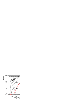
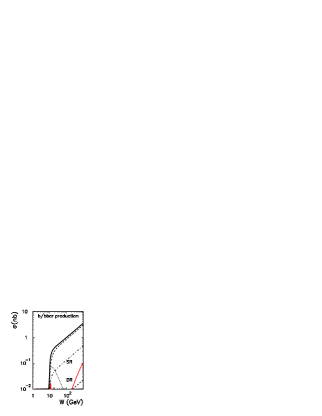
Figure 2: Different contributions to the inclusive charm (left panel) and bottom (right panel) production. The long-dashed line: the dipole-dipole contribution, the dash-dotted line: the single-resolved contribution, the lower dashed line: the $2Q2\bar{Q}$ contribution, the dotted line: the direct contribution, the gray solid line: double-resolved contribution. The experimental data for inclusive $c/\bar{c}$ production are from Ref.[9].

At higher energies the direct contribution is practically negligible. In contrast, the hadronic double-resolved contribution, when each of the two photons fluctuates into a vector meson [3] is shown by the thin solid line in the figure becomes important only at very high energies relevant for TESLA. Here we have consistently taken $g_{V}(x_{V},\mu_{F}^{2})=g_{\pi}(x_{V},\mu_{F}^{2})$.

The situation for bottom production (see right panel) is somewhat different. Here the main SAT-MOD component is dominant. Due to smaller charge of the bottom quark than that for the charm quark, the direct component is effectively reduced with respect to the dominant SAT-MOD component by the corresponding ratio of quark/antiquark charges: $(1/9)^{2}:(4/9)^{2}=1/16$. The same is true for the $2b2\bar{b}$ component. Here, in addition, there are threshold effects which play a role up to relatively high energy.

3.1 Short- versus long-distance phenomena

What are typical distances probed in heavy quark production ? Is the heavy quark production a short distance phenomenon ? These questions can be easily answered in the mixed representation formulation considered in the present paper. In Fig.3 I display the integrand of

$$\sigma_{\gamma\gamma\rightarrow c\bar{c}}(W)=\int\;I(\rho_{1},\rho_{2})\;d\rho_{1}d\rho_{2}\;.$$ (6)

The maxima in Fig.3 correspond to the most probable situations. For one light ($m_{u}$ = $m_{d}$ = $m_{0}$, $m_{s}$ = $m_{0}$ + 0.15 GeV) and second heavy quark-antiquark pair the map is clearly asymmetric. One can observe a ridge parallel to the $\rho_{1}$ or $\rho_{2}$ axis. There is no well localized maximum. Both short and long distances are probed.

Figure 3: A map of $\frac{d^{2}\sigma^{\gamma\gamma\rightarrow c\bar{c}}(\rho_{1},\rho_{2})}{d\rho_{1}d\rho_{2}}$ at W = 100 GeV for the first (left-top panel) and the second (right-top panel) photon fluctuating into $c\bar{c}$. For comparison I show analogous maps for light quark-antiquark pairs (left-bottom panel) and for the case when both pairs consist of charm quarks/antiquarks (right-bottom panel).

For comparison, in the bottom part of the figure, I show similar maps when both pairs consist of light (u,d,s) quarks/antiquarks (left-bottom) and in the case when both pairs consist of charm quarks/antiquarks (right-bottom). For light quarks (u,d,s) one observes a clear maximum at $(\rho_{1},\rho_{2})$ = (1 GeV^-1, 1 GeV^-1) = (0.2 fm, 0.2 fm). In this case a non-negligible strength extends, however, up to large distances $\rho_{1}$ and $\rho_{2}$. Only in the case of the production of two $c\bar{c}$ pairs, the cross section is dominated exclusively by short-distance phenomena.

3.2 $e^{+}e^{-}\rightarrow e^{+}e^{-}b\bar{b}X$

Up to now no attempt was done to unfold experimentally the cross section for $\gamma\gamma\rightarrow b\bar{b}X$. Only the cross section for the $e^{+}e^{-}\rightarrow b\bar{b}X$ reaction was obtained recently by the L3 and OPAL collaborations at LEP2 [9, 10]. The measured, positron and electron antitagged cross sections cannot be described as a sum of direct and single-resolved contributions, even if next-to-leading order corrections are included [10]. The measured cross section exceeds the theoretical predictions by a large factor. This is a new situation in comparison to the charm production where the deficit is much smaller.

The cross section for the $e^{+}e^{-}\rightarrow b\bar{b}\;X$ reaction when both positron and electron are antitagged can be easily estimated in the equivalent photon approximation (EPA) as

$$\sigma(e^{+}e^{-}\rightarrow b\bar{b}X;W_{ee})=\int dx_{A}dx_{B}\;f_{A}(E_{b},\theta_{max},x_{A})f_{B}(E_{b},\theta_{max},x_{B})$$

$$\sigma(\gamma\gamma\rightarrow b\bar{b}X;W)\;,$$ (7)

where $f_{A}$ and $f_{B}$ are virtuality-integrated flux factors of photons in the positron and electron, respectively, and $\theta_{max}$ is the maximal angle of the positron/electron not, to be identified by the experimental apparatus. In the present analysis we calculate the integrated flux factors $f_{A}$ and $f_{B}$ in a simple logarithmic approximation. The photon-photon energy can be calculated in terms of photon longitudinal momentum fractions $x_{A}$ and $x_{B}$ in the positron and electron, respectively, as $W=\sqrt{x_{A}x_{B}s_{ee}}$. It is instructive to visualize how different regions of $W_{\gamma\gamma}$ contribute to $\sigma(e^{+}e^{-}\rightarrow b\bar{b}X;W_{ee})$. For this purpose it is useful to transform variables from $x_{A},x_{B}$ to $x_{F}\equiv x_{A}-x_{B}$ and $W_{\gamma\gamma}=W$. Then

$$\sigma(e^{+}e^{-}\rightarrow b\bar{b}X;W_{ee})=\int dx_{F}dW\;{\cal J}\;f_{A}(E_{b},\theta_{max},x_{A})f_{B}(E_{b},\theta_{max},x_{B})$$

$$\sigma(\gamma\gamma\rightarrow b\bar{b}X;W)\;,$$ (8)

where the Jacobian ${\cal J}$ is a simple function of kinematical variables.

Figure 4: The dependence of the integrand of Eq.(7) on the photon-photon energy $W_{\gamma\gamma}$ for $x_{F}$ = 0 (solid) and $x_{F}$ = $\pm$ 0.5 (dashed) for the $b\bar{b}$ production for the direct mechanism (left panel) and in the dipole-dipole scattering in the Saturation Model (right panel) with the present prescription for the energy dependence of the dipole-dipole cross section. In this calculation $W_{ee}$ = 190 GeV.

The integrand $I(x_{F},W)$ of (8) for $b\bar{b}$ is shown in Fig.4 for the direct production (left panel) and for the Saturation Model (right panel) including all contributions considered in the present analysis. Quite a different pattern can be observed for the two mechanisms. While for the direct production one is sensitive mainly to low-energy photon-photon collisions, in the Saturation Model the contributions of high-energies cannot be neglected and one has to integrate over $W_{\gamma\gamma}$ essentially up to $W_{ee}$. This difference in $W_{\gamma\gamma}$ is due to different energy dependence of $\sigma(\gamma\gamma\rightarrow b\bar{b};W_{\gamma\gamma})$ for the different mechanisms considered, as has been discussed above. Even in the latter case the integrated cross section is very sensitive to the region of not too high energies $W\sim$ 20 GeV, where the not-fully-understood threshold effects may play essential role.

Table 1: Cross sections in pb for $e^{+}e^{-}\rightarrow b\bar{b}X$ for LEP2 averaged energy $W_{ee}$ = 190 GeV.

direct	$b\bar{b}$	$2b2\bar{b}$	SR	sum	L3	OPAL
	SAT-MOD	SAT-MOD	SAT-MOD
1.21	6.1-7.4	0.034	1.92	9.3-10.6	13.1 $\pm$ 2.0 $\pm$ 2.4	14.2 $\pm$ 2.5 $\pm$ 5.0

For LEP2 averaged energy $<W_{ee}>\approx$ 190 GeV the cross section integrated taking into account experimental cuts is $\sigma(e^{+}e^{-}\rightarrow b\bar{b}X)$ = 6.1 pb (C = 1) or 7.4 pb (C = 1/2) [3] for the dipole-dipole SAT-MOD scattering process. The corresponding cross section for the direct production is $\sigma(e^{+}e^{-}\rightarrow b\bar{b}X)$ = 1.2 pb. The hadronic single-resolved contribution calculated here in the Saturation Model is very similar in size to that calculated in the standard collinear approach [10]. As can be seen in Table 1 the $2b2\bar{b}$ contribution is practically negligible. We have completely omitted the double-resolved contribution which is practically negligible. The sum of the direct, $b\bar{b}$ SAT-MOD, $2b2\bar{b}$ SAT-MOD and the hadronic single resolved SAT-MOD component is 9.3-10.6 pb in the case when no transverse momenta cuts on the main SAT-MOD component are included and 6.4-7.1 pb with the cuts. These numbers should be compared to experimentally measured $\sigma(e^{+}e^{-}\rightarrow b\bar{b}X)$ = 13.1 $\pm$ 2.0 (stat) $\pm$ 2.4 (syst) pb [11] (L3) and preliminary $\sigma(e^{+}e^{-}\rightarrow b\bar{b}X)$ = 14.2 $\pm$ 2.5 (stat) $\pm$ 5.0 (syst) pb [11] (OPAL). In comparison to earlier calculations in the literature, the theoretical deficit is much smaller. The success of the present calculation relies on the inclusion of a few mechanisms neglected so far - in particular the dipole-dipole contribution which, in our opinion, is not contained in the standard collinear approach.

Up to now only the $W_{\gamma\gamma}$-integrated cross section has been determined experimentally. This, in fact, does not allow to identify experimentally whether the problem is in low or high $W_{\gamma\gamma}$. In order to identify better the region where the standard collinear approach fails it would be useful to bin the experimental cross section in the intervals of $W_{\gamma\gamma}$ making use of a possibility to measure $W_{vis}$ which can be related to $W_{\gamma\gamma}$ via a suitable Monte Carlo program. At present, even splitting the cross section for $e^{+}e^{-}\rightarrow b\bar{b}X$ into $\sigma(W_{\gamma\gamma}<W_{0})$ and $\sigma(W_{\gamma\gamma}>W_{0})$ for $W_{0}\sim$ 20 GeV would be useful and should shed more light on the problem of the experimental excess of $b\bar{b}$ relative to the “standard” QCD approach.

3.3 Quark-antiquark correlations

So far mainly the integrated cross section for heavy quark/antiquark production was considered in the literature. Only in a few cases inclusive distributions in transverse momentum or rapidity (see e.g.[12]) were presented. No attempts have so far been made to analyze the final state in more detail. In our opinion investigating correlations between heavy quark - heavy antiquark could be much more conclusive in identifying the production mechanisms than the integrated cross section or even a single variable distribution.

In principle, any correlation between two kinematical variables of the final quark and antiquark would be of interest. We suggest that the following final quark/antiquark momentum fractions:

$$x_{Q}=\frac{\vec{p}_{Q}}{|\vec{p}_{Q}|}{\hat{n}}_{\gamma_{1}}\;,$$

$$x_{\bar{Q}}=\frac{\vec{p}_{\bar{Q}}}{|\vec{p}_{\bar{Q}}|}{\hat{n}}_{\gamma_{1}}\;,$$ (9)

where

$${\hat{n}_{\gamma_{1}}}=\frac{\vec{p}_{\gamma_{1}}}{|\vec{p}_{\gamma_{1}}|}$$ (10)

would be very useful to separate the different mechanisms (approaches). In the definition above $\vec{p}_{Q}$ and $\vec{p}_{\bar{Q}}$ are momenta of the heavy quark and antiquark, respectively, and $\vec{p}_{\gamma_{1}}$ is the momentum of the first photon, all in the photon-photon center-of-mass frame. By definition -1 $<x_{Q},x_{\bar{Q}}<$ 1. Similar quantities are being used at present when analyzing, e.g., jet production at HERA to separate out resolved and direct processes.

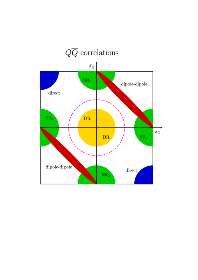
Figure 5: The expected locii in $(x_{Q},x_{\bar{Q}})$ space of different mechanisms considered in the present analysis. $SR_{1}$ / $SR_{2}$ means that the first/second photon was transformed into vector mesons and $DR$ means that each of the photons was transformed into a vector meson. The dashed circle is the locus corresponding to the pairs emitted from the middle of the gluonic ladder (not discussed in the text).

In Fig.5 I present a sketch of naive expectations. Although a precise map requires detailed calculations for each mechanism separately, which is beyond the scope of the present analysis, it is obvious that the separation of different mechanisms here should be much better than for any inclusive spectra. In the case of dipole-dipole approach (the elongated ellipses) this would require going to the momentum representation. The mixed representation used in the present paper is useful only for integrated cross sections.

Experimentally, the analysis suggested would be difficult at LEP2 because of rather limited statistics. We hope that such an analysis will be possible at the photon-photon option at TESLA. At present, even localizing a few LEP2 coincidence $c\bar{c}$ events in the diagram $x_{c}$ versus $x_{\bar{c}}$ would be instructive.

4 Conclusions

There is no common consensus in the literature on detailed understanding of the dynamics of photon-nucleon and photon-photon collisions. In this presentation I have limited the discussion to the production of heavy quarks simultaneously in photon-nucleon and photon-photon collisions at high energies. The sizeable mass of charm or bottom quarks sets a natural low energy limit on a naive application of SAT-MOD. Here a careful treatment of the kinematical threshold is required.

We have started the analysis from (real) photon-nucleon scattering, which is very close to the domain of SAT-MOD as formulated in [1]. If the kinematical threshold corrections are included, SAT-MOD gives similar results as the standard collinear approach for both charm and bottom production. We have estimated the VDM contribution to the heavy quark production.

The second part of the present analysis has been devoted to real photon - real photon collisions. For the first time in the literature we have estimated the cross section for the production of $2c2\bar{c}$ final state. We have found that this component constitutes up to 10-15 % of the inclusive charm production at high energies and is negligible for the bottom production. We have shown how to generalize SM to the case when one of the photons fluctuates into light vector mesons. It was found that this component yields a significant correction of about 30-40 % for inclusive charm production and 15-20 % for bottom production. We have shown that the double resolved component, when both photons fluctuate into light vector mesons, is nonnegligible only at very high energies, both for the charm and bottom production.

I have shown that the production of $c\bar{c}$ pairs (the same is true for $b\bar{b}$) is not completely of perturbative character and involves both short- and large-size contributions. The latter as nonperturbative are unavoidably subjected to some modeling. Present experimental statistics do not allow extraction of cross sections for the $\gamma\gamma\rightarrow b\bar{b}$ reaction and therefore it is not clear where the observed deficit resides. It is not excluded that the apparent deficit of bottom quarks may reside at photon-photon energies close to threshold. This is a region where the underlying physics has never carefully been studied.

Finally I have discussed a possibility to distinguish experimentally the different mechanisms discussed in the present paper by measuring heavy quark - antiquark correlations. This suggestion requires, however, further detailed studies of the Monte Carlo type, including experimental possibilities and limitations.

The present calculation is not fully consistent as far as parameters are considered. I have taken SAT-MOD parameters from Ref.[1], where only dipole (quark-antiquark) component was fitted to the total cross section for $\gamma^{*}p$ scattering and added the resolved photon in addition. In a consistent treatment one should include in addition the resolved photon component in the fit to the HERA structure function data. Such an analysis has been completed only recently [13].

References

- [1] K. Golec-Biernat and M. Wüsthoff, Phys. Rev. D59 (1998) 014017.
- [2] N. Timneanu, J. Kwieciński and L. Motyka, Eur. Phys. Jour. C23 (2002) 513.
- [3] A. Szczurek, Eur. Phys. Jour. C26 (2002) 183.
- [4] N.N. Nikolaev and B.G. Zakharov, Z. Phys. C49 (1991) 607.
- [5] S. Aid et al.(H1 collaboration), Nucl. Phys.B472 (1996) 32.
- [6] C. Adloff et al. (H1 collaboration), Phys. Lett. B467 (1999) 156.
- [7] M. Glück, E. Reya and A. Vogt, Z. Phys. C53 (1992) 651.
- [8] M. Glück, E. Reya and A. Vogt, Z. Phys. C67 (1995) 433.
- [9] M. Acciarri et al.(L3 collaboration), Phys. Lett. B514 (2001) 19.
- [10] A. Csilling, hep-ex/0010060, a talk given at the conference PHOTON2000, Ambleside, UK, August 2000.
- [11] M. Acciarri et al.(L3 collaboration), Phys. Lett. B503 (2001) 10.
- [12] M. Krämer and E. Laenen, Phys. Lett. B371 (1996) 303.
-
[13]
A. Szczurek, a talk at the international workshop DIS2003,
Sankt Petersburg, Russia, April 23-27, 2003;
T. Pietrycki and A. Szczurek, hep-ph/0306009.