How to reconcile the Rosenbluth and the polarization transfer methods in the measurement of the proton form factors

Abstract

The apparent discrepancy between the Rosenbluth and the polarization transfer method for the ratio of the electric to magnetic proton form factors can be explained by a two-photon exchange correction which does not destroy the linearity of the Rosenbluth plot. Though intrinsically small, of the order of a few percent of the cross section, this correction is accidentally amplified in the case of the Rosenbluth method.

The electro-magnetic form factors are essential pieces of our knowlegde of the nucleon structure and this justifies the efforts devoted to their experimental determination. They are defined as the matrix elements of the electro-magnetic current $J^{\mu}(x)$ according to  :

$$<N(p^{\prime})|J^{\mu}(0)|N(p)>$$

$$=\,e\,\bar{u}(p^{\prime})\left[G_{M}(Q^{2})\gamma^{\mu}-F_{2}(Q^{2})\frac{(p+p^{\prime})^{\mu}}{2M}\right]u(p),$$ (1)

where $e\simeq\sqrt{4\pi/137}$ is the proton charge, $M$ the nucleon mass, and $Q^{2}$ the squared momentum transfer. The magnetic form factor $G_{M}$ is related to the Dirac ($F_{1})$ and Pauli ($F_{2})$ form factors by $G_{M}=F_{1}+F_{2}$, and the electric form factor is given by $G_{E}=F_{1}-\tau F_{2}$, with $\tau=Q^{2}/4M^{2}$. For the proton, $F_{1}(0)=1$, and $F_{2}(0)=\mu_{p}-1=1.79$. In the one-photon exchange or Born approximation, elastic lepton-nucleon scattering :

$$l(k)+N(p)\rightarrow l(k^{\prime})+N(p^{\prime}),$$ (2)

gives direct access to the form factors in the spacelike region ($Q^{2}>0)$, through its cross section :

$$d\sigma_{B}=C_{B}(Q^{2},\varepsilon)\left[G_{M}^{2}(Q^{2})+\frac{\varepsilon}{\tau}G_{E}^{2}(Q^{2})\right],$$ (3)

where $\varepsilon$ is the photon polarization parameter, and $C_{B}(Q^{2},\varepsilon)$ is a phase space factor which is irrelevant in what follows. For a given value of $Q^{2}$, Eq. (3) shows that it is sufficient to measure the cross section for two values of $\varepsilon$ to determine the form factors $G_{M}$ and $G_{E}$. This is referred to as the Rosenbluth method Rosenb50 . The fact that $d\sigma/C_{B}(Q^{2},\varepsilon)$ is a linear function of $\varepsilon$ (Rosenbluth plot criterion) is generally considered as a test of the validity of the Born approximation.
Polarized lepton beams give another way to access the form factors Akhieser58 . In the Born approximation, the polarization of the recoiling proton along its motion ($P_{l}$) is proportional to $G_{M}^{2}$ while the component perpendicular to the motion ($P_{t}$ ) is proportional to $G_{E}G_{M}$. We call this the polarization method for short. Because it is much easier to measure ratios of polarizations, it has been used mainly to determine the ratio $G_{E}/G_{M}$ through a measurement of $P_{t}/P_{l}$ using Akhiezer68  :

$$\frac{P_{t}}{P_{l}}=-\sqrt{\frac{2\varepsilon}{\tau(1+\varepsilon)}}\frac{G_{E}}{G_{M}}.$$ (4)

Thus, in the framework of the Born approximation, one has two independent measurements of $R=G_{E}/G_{M}.$ In Fig. 1 we show the corresponding results, which we call $R^{exp}_{Rosenbluth}$ and $R^{exp}_{Polarization}$ , for the range of $Q^{2}$ which is common to both methods. The data are from Refs. LT1994 ; Jones00 ; Gayou02 . It is seen that the deviation between the two methods starts around $Q^{2}=2$ GeV² and increases with $Q^{2}$, reaching a factor $4$ at $Q^{2}=6$ GeV². A recent re-analysis of the SLAC cross sections Arr03 and new Rosenbluth measurements from JLab Chr03 confirm that the Rosenbluth and polarization extractions of the ratio $G_{E}/G_{M}$ are incompatible at large $Q^{2}$. This discrepancy is a serious problem as it generates confusion and doubt about the whole methodology of lepton scattering experiments.
In this letter we take a first step to unravel this problem by interpreting the discrepancy as a failure of the Born approximation which nevertheless does not destroy the linearity of the Rosenbluth plot. This means that we give up the beloved one-photon exchange concept and enter the not well paved path of multi-photon physics. By this we do not mean the effect of soft (real or virtual) photons, that is the radiative corrections. The effect of the latter is well under control because their dominant (infra-red) part can be factorized in the observables and therefore does not affect the ratio $G_{E}/G_{M}$. Here we consider genuine exchange of hard photons between the lepton and the hadron. Such higher-order corrections to the one-photon exchange approximation have been considered in the past Dr59 ; Gr69 , and their effects were found to be of order 1 - 2 % on the cross section. However, such estimates based on nucleon and resonance intermediate states can only be expected to give a realistic description of the nucleon structure for momentum transfers up to $Q^{2}\lesssim 1$ GeV², whereas they are largely unknown at higher values of $Q^{2}$.

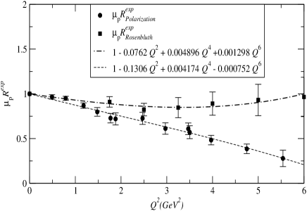
Figure 1: Experimental values of $R^{exp}_{Rosenbluth}$ LT1994 and $R^{exp}_{Polarization}$ Jones00 ; Gayou02 and their polynomial fits.

Even if we restrict ourselves to the two-photon exchange case, the evaluation of the box diagram (Fig. 2) involves the full reponse of the nucleon to doubly virtual Compton scattering and we do not know how to perform this calculation in a model independent way. Therefore we adopt a modest strategy based on the phenomenological consequences of using the full $eN$ scattering amplitude rather than its Born approximation. Though it cannot lead to a full answer it produces the following interesting results:

• the two-photon exchange amplitude needed to explain the discrepancy is actually of the expected order of magnitude, that is a few percent of the Born amplitude.

• there may be a simple explanation of the fact that the Rosenbluth plot looks linear even though it is strongly affected by the two-photon exchange.

• the polarization method result is little affected by the two-photon exchange, at least in the range of $Q^{2}$ which has been studied until now.

Figure 2: The box diagram. The filled blob represents the response of the nucleon to the scattering of the virtual photon.

To proceed with the general analysis of elastic electron-nucleon scattering (2), we adopt the usual definitions :

$$P=\frac{p+p^{\prime}}{2},\,K=\frac{k+k^{\prime}}{2},\,q=k-k^{\prime}=p^{\prime}-p,$$ (5)

and choose

$$Q^{2}=-q^{2},\,\nu=K.P,$$ (6)

as the independent invariants of the scattering. The polarization parameter $\varepsilon$ of the virtual photon is related to the invariant $\nu$ as (neglecting the electron mass $m_{e}$) :

$$\varepsilon=\frac{\nu^{2}-M^{4}\tau(1+\tau)}{\nu^{2}+M^{4}\tau(1+\tau)}.$$ (7)

For a theory which respects Lorentz, parity and charge conjugation invariance, the $T$-matrix for elastic scattering of two spin 1/2 particles can be expanded in terms of six independent Lorentz structures which, following Ref. Goldb57 , can be chosen as: $\bar{u}(k^{\prime})u(k)\ \bar{u}(p^{\prime})u(p)$, $\bar{u}(k^{\prime})u(k)\ \bar{u}(p^{\prime})\gamma.Ku(p)$, $\bar{u}(k^{\prime})\gamma_{5}u(k)\ \bar{u}(p^{\prime})\gamma_{5}u(p)$, $\bar{u}(k^{\prime})\gamma.Pu(k)\ \bar{u}(p^{\prime})\gamma.Ku(p)$, $\bar{u}(k^{\prime})\gamma.Pu(k)\ \bar{u}(p^{\prime})u(p)$, $\bar{u}(k^{\prime})\gamma_{5}\gamma.Pu(k)\ \bar{u}(p^{\prime})\gamma_{5}\gamma.Ku(p)$. In the limit $m_{e}\to 0$, the vector nature of the coupling in QED implies that any Feynman diagram is invariant under the chirality operation $u(k)\to\gamma_{5}u(k),\bar{u}(k^{\prime})\to-\bar{u}(k^{\prime})\gamma_{5}$. Therefore the Lorentz structures which change their sign under this operation must come with an explicit factor $m_{e}$. This allows us to neglect the structures which contain either $\bar{u}(k^{\prime})u(k)$ or $\bar{u}(k^{\prime})\gamma_{5}u(k)$. Using the Dirac equation and elementary relations between Dirac matrices the linear combination of the remaining three amplitudes can be written in the form :

$$T\, = \,\frac{e^{2}}{Q^{2}}\,\bar{u}(k^{\prime})\gamma_{\mu}u(k)\,$$ (8)

$$\times \bar{u}(p^{\prime})\left(\tilde{G}_{M}\,\gamma^{\mu}-\tilde{F}_{2}\frac{P^{\mu}}{M}+\tilde{F}_{3}\frac{\gamma.KP^{\mu}}{M^{2}}\right)u(p),$$

where $\tilde{G}_{M},\,\tilde{F}_{2},\,\tilde{F}_{3}$ are complex functions of $\nu$ and $Q^{2}$, and where the factor $e^{2}/Q^{2}$ has been introduced for convenience. In the Born approximation, one obtains :

$$\tilde{G}_{M}^{Born}(\nu,Q^{2})\, = \,G_{M}(Q^{2}),$$

$$\tilde{F}_{2}^{Born}(\nu,Q^{2})\, = \,F_{2}(Q^{2}),$$

$$\tilde{F}_{3}^{Born}(\nu,Q^{2})\, = \,0.$$ (9)

Since $\tilde{F}_{3}$ and the phases of $\tilde{G}_{M}$ and $\tilde{F}_{2}$ vanish in the Born approximation, they must originate from processes involving at least the exchange of two photons. Relative to the factor $e^{2}$ introduced in Eq. (8), we see that they are at least of order $e^{2}.$ This, of course, assumes that the phases of $\tilde{G}_{M}$ and $\tilde{F}_{2}$ are defined, which amounts to supposing that, in the kinematical region of interest, the moduli of $\tilde{G}_{M}$ and $\tilde{F}_{2}$ do not vanish, which we take for granted in the following. Defining :

$$\tilde{G}_{M}=e^{i\phi_{M}}|\tilde{G}_{M}|,\,\tilde{F}_{2}=e^{i\phi_{2}}|\tilde{F}_{2}|,\,\tilde{F}_{3}=e^{i\phi_{3}}|\tilde{F}_{3}|,$$ (10)

and using standard techniques, we get the following expressions for the observables of interest :

$$d\sigma = C_{B}(\nu,Q^{2})\,\frac{\varepsilon(1+\tau)}{\tau}$$ (11)

$$\times \left\{|\tilde{G}_{M}|^{2}\,\frac{\rho^{2}-\tau+\tau^{2}}{\rho^{2}-\tau-\tau^{2}}+|\tilde{F}_{2}|^{2}(1+\tau)\right.$$

$$-2\,|\tilde{G}_{M}|\,\left(\cos\phi_{2M}|\tilde{F}_{2}|-\cos\phi_{3M}|\tilde{F}_{3}|\rho\right)$$

$$\left.-2\,\cos\phi_{23}\,|\tilde{F}_{2}\tilde{F}_{3}|\rho+|\tilde{F}_{3}|^{2}(\rho^{2}-\tau^{2})\right\},$$

$$\frac{P_{t}}{P_{l}} = -\sqrt{\frac{\rho^{2}-\tau-\tau^{2}}{\tau}}$$

$$\times \frac{|\tilde{G}_{M}|-\cos\phi_{2M}|\tilde{F}_{2}|(1+\tau)+\cos\phi_{3M}|\tilde{F}_{3}|\rho}{|\tilde{G}_{M}|\rho+\cos\phi_{3M}|\tilde{F}_{3}|(\rho^{2}-\tau-\tau^{2})},$$ (12)

with $\phi_{2M}=\phi_{2}-\phi_{M}$, $\phi_{3M}=\phi_{3}-\phi_{M}$, $\phi_{23}=\phi_{2}-\phi_{3}$, and $\rho=\nu/M^{2}$. If one substitutes the Born approximation values of the amplitudes (How to reconcile the Rosenbluth and the polarization transfer methods in the measurement of the proton form factors) then Eqs. (11,12) give back the familiar expressions of Eqs. (3,4).
To simplify the above general expressions, we make the very reasonable assumption that only the two-photon exchange needs to be considered. In practice we make an expansion in power of $e^{2}$ of Eqs. (11,12) using the fact that $\phi_{M},\,\phi_{2}$ and $\tilde{F}_{3}$ are at least of order $e^{2}$ but we do not expand $|\tilde{G}_{M}|$ and $|\tilde{F}_{2}|$, which is perfectly legitimate. This leads to the following approximate expressions :

$$\frac{d\sigma}{C_{B}(\varepsilon,Q^{2})} \simeq \frac{|\tilde{G}_{M}|^{2}}{\tau}\left\{\tau+\varepsilon\frac{|\tilde{G}_{E}|^{2}}{|\tilde{G}_{M}|^{2}}\right.$$ (13)

$$\left.+\,2\varepsilon\left(\tau+\frac{|\tilde{G}_{E}|}{|\tilde{G}_{M}|}\right){\cal R}\left(\frac{\nu\tilde{F}_{3}}{M^{2}|\tilde{G}_{M}|}\right)\right\},$$

$$\frac{P_{t}}{P_{l}} \simeq -\,\sqrt{\frac{2\varepsilon}{\tau(1+\varepsilon)}}\,\left\{\,\frac{|\tilde{G}_{E}|}{|\tilde{G}_{M}|}\right.$$ (14)

$$\left.+\left(1-\frac{2\varepsilon}{1+\varepsilon}\frac{|\tilde{G}_{E}|}{|\tilde{G}_{M}|}\right){\cal R}\left(\frac{\nu\tilde{F}_{3}}{M^{2}|\tilde{G}_{M}|}\right)\right\},$$

where the neglected terms are of order $e^{4}$ w.r.t. the leading one. By analogy, we have defined :

$$\tilde{G}_{E}=\tilde{G}_{M}-(1+\tau)\tilde{F}_{2},\,$$ (15)

and ${\cal R}$ denotes the real part. Note that $\tilde{G}^{Born}_{E}(\nu,Q^{2})=G_{E}(Q^{2})$. To set the scale for the size of the two-photon exchange term $(\tilde{F}_{3})$ we introduce the dimensionless ratio :

$$Y_{2\gamma}(\nu,Q^{2})={\cal R}\left(\frac{\nu\tilde{F}_{3}}{M^{2}|\tilde{G}_{M}|}\right).$$ (16)

In the region of large $Q^{2}$ which is where the discrepancy really gets large, $\tau$ is of order 1 or larger, while we can take as upper bound estimate $|\tilde{G}_{E}|/|\tilde{G}_{M}|\simeq G_{E}(0)/G_{M}(0)=1/2.79$ . So, for a qualitative reasoning, we can neglect $|\tilde{G}_{E}|/|\tilde{G}_{M}|$ with respect to $\tau$ and, up to a term quadratic in $Y_{2\gamma}$, the cross section has the form $|\tilde{G}_{M}|^{2}(1+\varepsilon\,Y_{2\gamma})^{2}$. So we expect $Y_{2\gamma}\sim\alpha\simeq 1/137$. However in the Rosenbluth method where one identifies $(G_{E}/G_{M})^{2}$ with the coefficient of $\varepsilon$, the two photon effect comes as a correction to a small number $\sim(1/2.79)^{2}$. So we expect that the correction will have a stronger effect in the Rosenbluth than in the polarization method.
From Eqs. (13,14) we see that the pair of observables $(d\sigma,\,P_{t}/P_{l})$ depends on $|\tilde{G}_{M}|$, $|\tilde{G}_{E}|$, and ${\cal R}(\tilde{F}_{3})$. In the first approximation, we know that $|\tilde{G}_{M}(\nu,Q^{2})|\simeq G_{M}(Q^{2})$, $|\tilde{G}_{E}(\nu,Q^{2})|\simeq G_{E}(Q^{2})$, and only ${\cal R}(\tilde{F}_{3})$ is really a new unknown parameter. Thus allowing for two-photon exchange somewhat complicates the interpretation of the lepton scattering experiments but not in a dramatic way. The main uncertainty is the dependence on $\nu$ (or $\varepsilon$) of $\tilde{F}_{3}$ and to further simplify the problem we make the following observations. First, if we look at the data of Ref. LT1994 for $d\sigma/C_{B}(\varepsilon,Q^{2})$ as a function of $\varepsilon$ we observe that for each value of $Q^{2}$ the set of points are pretty well aligned. We see in Eq. (13) that this can be understood if, at least in the first approximation, the product $\nu\,\tilde{F}_{3}$ is independent of $\varepsilon.$ We do not have a first principle explanation for this but we feel allowed to take it as experimental evidence. To explain the linearity of the plot one must also suppose that $|\tilde{G}_{M}|$ and $|\tilde{G}_{E}|$ are independent of $\varepsilon$ (that is $\nu$ ) but since the dominant term of these amplitudes depends only on $Q^{2}$ this is a very mild assumption. We then see from Eq. (13) that what is measured using the Rosenbluth method is :

$$(R^{exp}_{Rosenbluth})^{2}=\frac{|\tilde{G}_{E}|^{2}}{|\tilde{G}_{M}|^{2}}+2\left(\tau+\frac{|\tilde{G}_{E}|}{|\tilde{G}_{M}|}\right)Y_{2\gamma},$$ (17)

with $|\tilde{G}_{E}|/|\tilde{G}_{M}|$ and $Y_{2\gamma}$ essentially independent of $\varepsilon$ , rather than $(R^{exp}_{Rosenbluth})^{2}=(G_{E}/G_{M})^{2}$ , as implied by one-photon exchange. Second, the experimental results of the polarization method have been obtained for a rather narrow range of $\varepsilon$, typically from $\varepsilon=0.75$ to $0.9$ for the points at large $Q^{2}$. So, in practice, we can neglect the $\varepsilon$ dependence of $R^{exp}_{Polarization}$ and from Eq. (14) we see that this experimental ratio must be interpreted as :

$$R^{exp}_{Polarization}=\frac{|\tilde{G}_{E}|}{|\tilde{G}_{M}|}+\left(1-\frac{2\varepsilon}{1+\varepsilon}\frac{|\tilde{G}_{E}|}{|\tilde{G}_{M}|}\right)Y_{2\gamma},$$ (18)

rather than $R^{exp}_{Polarization}=G_{E}/G_{M}$. In order that Eq. (18) be consistent with our hypothesis we should find that $Y_{2\gamma}$ is small enough that the factor $2\varepsilon/(1+\varepsilon)$ introduces no noticeable $\varepsilon$ dependence in $R^{exp}_{Polarization}$.

Figure 3: The ratio $Y^{exp}_{2\gamma}$ versus $\varepsilon$ for several values of $Q^{2}$.

We can now solve Eqs. (17,18) for $|\tilde{G}_{E}|/|\tilde{G}_{M}|$ and $Y_{2\gamma}$ for each $Q^{2}$ . Since the system of equations is equivalent to a quadratic equation it is more efficient to solve it numerically. For this we have fitted the data by a polynomial in $Q^{2}$ as shown in Fig. 1, and we shall consider this fit as the experimental values. In particular we do not attempt to represent the effect of the error bars which can be postponed to a more complete re-analysis of the data. The solution of Eqs. (17,18) for the ratio $Y^{exp}_{2\gamma}$ is shown in Fig. 3 where we can see that, as expected, it is essentially flat as a function of $\varepsilon$ and small, of the order of a few percent. Thus a tiny correction allows the Rosenbluth and the polarization method to give the same value for $|\tilde{G}_{E}|/|\tilde{G}_{M}|$. It is reasonable to think that $\delta G_{E}=\tilde{G}_{E}-G_{E}$ and $\delta G_{M}=\tilde{G}_{M}-G_{M}$ are comparable to $Y^{exp}_{2\gamma}$ and therefore $|\tilde{G}_{E}|/|\tilde{G}_{M}|$ should not be very different from the actual value of $G_{E}/G_{M}$. So it makes sense to compare the value we get for $R^{exp}_{1\gamma+2\gamma}=|\tilde{G}_{E}|/|\tilde{G}_{M}|$ with the starting experimental ratios $R^{exp}_{Rosenbluth}$ and $R^{exp}_{Polarization}$. This is shown in Fig. 4, from which we see that $R^{exp}_{1\gamma+2\gamma}$ is close to $R^{exp}_{Polarization}$. The difference between the two curves can be attributed either to $Y^{exp}_{2\gamma}$ or to $(\delta G_{M},\ \delta G_{E})$. Insofar as $(\delta G_{M},\ \delta G_{E})$ are of the same order of magnitude as $Y^{exp}_{2\gamma}$, which is small according to our analysis, our interpretation of this small difference is that the polarization method is little affected by the two-photon correction.
In summary, the discrepancy between the Rosenbluth and the polarization method for $G_{E}/G_{M}$ can be attributed to a failure of the one-photon approximation which is amplified at large $Q^{2}$ in the case of the Rosenbluth method. The expression for the cross section also suggests that the two-photon effect does not destroy the linearity of the Rosenbluth plot provided the product ${\cal R}(\nu\tilde{F}_{3})$ is independent of $\nu.$ It remains to be investigated if there is a fundamental reason for this behavior or if it is fortuitous. Using the existing data we have extracted the essential piece of the puzzle, that is the ratio $Y^{exp}_{2\gamma}$ which measures the relative size of the two-photon amplitude $\tilde{F}_{3}$. Within our approximation scheme, we find that $Y^{exp}_{2\gamma}$ is of the order of a few percent. This is a very reassuring result since this is the order of magnitude expected for two-photon corrections. What is needed next is a realistic evaluation of this particular amplitude. A first step in this direction was performed very recently in Ref. Blund03 , where the contribution to the two-photon exchange amplitude was calculated for a nucleon intermediate state in Fig. 2. The calculation of Ref. Blund03 found that the two-photon exchange correction with intermediate nucleon has the proper sign and magnitude to resolve a large part of the discrepancy between the two experimental techniques, confirming the finding of our general analysis. As a next step, an estimate of the inelastic part is needed to fully quantify the nucleon response in the two-photon exchange process.
From our analysis we extract the ratio $|\tilde{G}_{E}|/|\tilde{G}_{M}|$ which in the first approximation should not be very different from $G_{E}/G_{M}$. We find that it is close to the value obtained by the polarization method when one assumes the one-photon exchange approximation. This comparison is meaningful if, as suggested by the smallness of $Y^{exp}_{2\gamma}$, $\delta G_{E}$ and $\delta G_{M}$ are negligible. This could be checked by a realistic calculation of the two-photon corrections. However we think that a definitive conclusion will wait for the determination of $\delta G_{E}$ and $\delta G_{M}$ as we did for $Y^{exp}_{2\gamma}$. The necessary experiments probably require the use of positrons as well as electron beams.

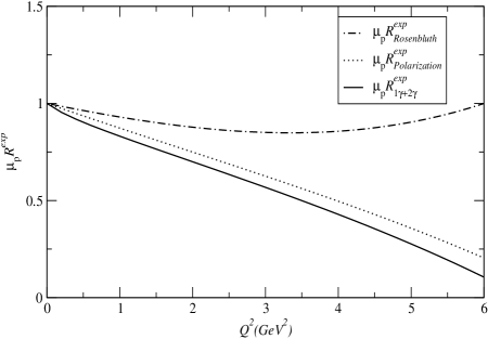
Figure 4: Comparison of the experimental ratios $\mu_{p}R^{exp}_{Rosenbluth}$ and $\mu_{p}R^{exp}_{Polarization}$ with the value of $\mu_{p}R^{exp}_{1\gamma+2\gamma}$ deduced from our analysis.

This work was supported by the French Commissariat à l’Energie Atomique (CEA), and by the Deutsche Forschungsgemeinschaft (SFB443).

References

- (1) M.N. Rosenbluth, Phys. Rev. 79, 615 (1950).
- (2) A.I. Akhiezer, L.N. Rozentsveig and I.M. Shmushkevich, Sov. Phys. JETP6, 588 (1958).
- (3) A.I. Akhiezer and M.P. Rekalo, Sov. Phys. Doklady 13, 572 (1968).
- (4) L. Andivahis et al., Phys. Rev. D 50, 5491 (1994).
- (5) M.K. Jones et al., Phys. Rev. Lett. 84, 1398 (2000).
- (6) O. Gayou et al., Phys. Rev. Lett. 88, 092301 (2002).
- (7) J. Arrington, nucl-ex/0305009.
- (8) M.C. Christy et al., to be submitted to Phys. Rev. C.
- (9) S.D. Drell and S. Fubini, Phys. Rev. 113, 741 (1959).
- (10) G.K. Greenhut, Phys. Rev. 184, 1860 (1969).
- (11) M.L. Goldberger, Y. Nambu and R. Oehme, Ann. of Phys. 2, 226 (1957).
- (12) P.G. Blunden, W. Melnitchouk and J.A. Tjon, nucl-th/0306076.