Nonfactorizable contributions to $B\rightarrow D^{(*)}M$ decays

Yong-Yeon Keum^a , T. Kurimoto^b, Hsiang-nan Li^c,d,
Cai-Dian Lü^e, and A.I. Sanda^a

^aDepartment of Physics, Nagoya University, Nagoya, Japan

^bFaculty of Science, Toyama University, Toyama 930-8555, Japan

^cInstitute of Physics, Academia Sinica, Taipei, Taiwan 115, Republic of China

^dDepartment of Physics, National Cheng-Kung University,
Tainan, Taiwan 701, Republic of China

^eCCAST (World Laboratory), P.O. Box 8730, Beijing 100080, China;

^eInstitute of High Energy Physics, CAS, P.O. Box 918(4), Beijing 100039, China

While the naive factorization assumption works well for many two-body nonleptonic $B$ meson decay modes, the recent measurement of $\bar{B}\rightarrow D^{(*)0}M^{0}$ with $M=\pi$, $\rho$ and $\omega$ shows large deviation from this assumption. We analyze the $B\rightarrow D^{(*)}M$ decays in the perturbative QCD approach based on $k_{T}$ factorization theorem, in which both factorizable and nonfactorizable contributions can be calculated in the same framework. Our predictions for the Bauer-Stech-Wirbel parameters, $\left|a_{2}/a_{1}\right|=0.43\pm 0.04$ and $Arg(a_{2}/a_{1})\sim-42^{\circ}$ and $\left|a_{2}/a_{1}\right|=0.47\pm 0.05$ and $Arg(a_{2}/a_{1})\sim-41^{\circ}$, are consistent with the observed $B\rightarrow D\pi$ and $B\rightarrow D^{*}\pi$ branching ratios, respectively. It is found that the large magnitude $|a_{2}|$ and the large relative phase between $a_{2}$ and $a_{1}$ come from color-suppressed nonfactorizable amplitudes. Our predictions for the ${\bar{B}}^{0}\rightarrow D^{*0}\rho^{0}$, $D^{*0}\omega$ branching ratios can be confronted with future experimental data.

1 INTRODUCTION

Understanding nonleptonic $B$ meson decays is crucial for testing the standard model, and also for uncovering the trace of new physics. The simplest case is two-body nonleptonic $B$ meson decays, for which Bauer, Stech and Wirbel (BSW) proposed the naive factorization assumption (FA) in their pioneering work [1]. Considerable progress, including generalized FA [2, 3, 4] and QCD-improved FA (QCDF) [5], has been made since this proposal. On the other hand, technique to analyze hard exclusive hadronic scattering was developed by Brodsky and Lepage [6] based on collinear factorization theorem in perturbative QCD (PQCD). A modified framework based on $k_{T}$ factorization theorem was then given in [7, 8], and extended to exclusive $B$ meson decays in [9, 10, 11, 12]. The infrared finiteness and gauge invariance of $k_{T}$ factorization theorem was shown explicitly in [13]. Using this so-called PQCD approach, we have investigated dynamics of nonleptonic $B$ meson decays [14, 15, 16]. Our observations are summarized as follows:

1. FA holds approximately for charmless $B$ meson decays, as our computation shows that nonfactorizable contributions are always negligible due to the cancellation between a pair of nonfactorizable diagrams.

2. Penguin amplitudes are enhanced, as the PQCD formalism includes dynamics from the region, where the energy scale $\mu$ runs to $\sqrt{\bar{\Lambda}m_{b}}<m_{b}$, $\bar{\Lambda}\equiv m_{B}-m_{b}$ being the $B$ meson and $b$ quark mass difference.

3. Annihilation diagrams contribute to large short-distance strong phases through the $(S+P)(S-P)$ penguin operators.

4. The sign and the magnitude of CP asymmetries in two-body nonleptonic $B$ meson decays can be calculated, and we have predicted relatively large CP asymmetries in the $B\rightarrow K^{(*)}\pi$ [14, 17] and $\pi\pi$ modes[15, 16, 18].

All analyses involving strong dynamics suffer large theoretical uncertainties than we would like. How reliable are these predictions? This can be answered only by comparing more of our predictions with experimental data. For this purpose, we study the $B\rightarrow D^{(*)}M$ decays in PQCD, where $M$ is a pseudoscalar or a vector meson. A $D^{(*)}$ meson is massive, and the energy release involved in two-body charmed decays is not so large. If predictions for these decays agree reasonably well with experimental data, PQCD should be more convincing for two-body charmless decays. Since penguin diagrams do not contribute, there are less theoretical ambiguities, such as the argument on chiral enhancement or dynamical enhancement. Checking the validity of PQCD analyses in charmed decays is then more direct.

Note that FA is expected to break down for charmed nonleptonic $B$ meson decays [19]. FA holds for charmless decays because of the color transparency argument: contributions from the dominant soft region cancel between the two nonfactorizable diagrams, where the exchanged gluons attach the quark and the antiquark of the light meson emitted from the weak vertex. For charmed decays with the light meson replaced by a $D^{(*)}$ meson, the two nonfactorizable amplitudes do not cancel due to the mass difference between the two constituent quarks of the $D^{(*)}$ meson. Hence, nonfactorizable contributions ought to be important. This observation further leads to the speculation that strong phases in the $B\rightarrow D^{(*)}M$ decays, if there are any, arise from nonfactorizable amplitudes. In charmless decays, strong phases come from annihilation amplitudes through the $(S+P)(S-P)$ penguin operators, since nonfactorizable ones are negligible as explained above. Annihilation amplitudes should not be the source of strong phases for charmed decays, which do not involve the $(S+P)(S-P)$ penguin operators.

In this paper we shall apply the PQCD formalism to the two-body charmed decays $B\rightarrow D^{(*)}M$ with $M=\pi$, $\rho$ and $\omega$. PQCD has predicted the strong phases from annihilation amplitudes for charmless decays, which are consistent with the recently measured CP asymmetries in the $B^{0}_{d}\rightarrow\pi^{+}\pi^{-}$ modes. It is then interesting to examine whether PQCD also gives the correct magnitude and strong phases from nonfactorizable amplitudes implied by the isospin relation of the $B\rightarrow D^{(*)}M$ decays. Compared to the work in [11], the contributions from the twist-3 light meson distribution amplitudes and the threshold resummation effect have been taken into account, and more modes analyzed. The power counting rules for charmed $B$ meson decays, constructed in [20], are employed to obtain the leading factorization formulas. It will be shown that nonfactorizable contributions to charmed decays are calculable in PQCD, and play an important role in explaining the isospin relation indicated by experimental data. The predictions for the $B\rightarrow D^{*0}\rho^{0}$, $D^{*0}\omega$ branching ratios can be confronted with future measurement.

In Sec. II we review the progresses on the study of two-body charmed nonleptonic $B$ meson decays in the literature. The PQCD analysis of the above decays is presented in Sec. III by taking the $B\rightarrow D\pi$ modes as an example. Numerical results for all the $B\rightarrow D^{(*)}M$ branching ratios, and for the extracted BSW parameters $a_{1}$ and $a_{2}$ are collected in Sec. IV. In Sec. V we compare the PQCD approach to exclusive $B$ meson decays with others in the literature. Sec. VI is the conclusion. Appendix A contains the explicit expressions of the factorization formulas.

2 REVIEW OF PREVIOUS WORKS

2.1 PQCD Approach to $B\rightarrow D^{(*)}$ Form Factors

To develop the PQCD formalism for charmed $B$ meson decays, we have investigated the $B\rightarrow D^{(*)}$ transition form factors in the large recoil region of the $D^{(*)}$ meson [20]. We briefly review this formalism, which serves as the basis of the $B\rightarrow D^{(*)}M$ analysis. The $B\rightarrow D^{(*)}$ transition is more complicated than the $B\rightarrow\pi$ one, because it involves three scales: the $B$ meson mass $m_{B}$, the $D^{(*)}$ meson mass $m_{D^{(*)}}$, and the heavy meson and heavy quark mass difference, $\bar{\Lambda}=m_{B}-m_{b}\sim m_{D^{(*)}}-m_{c}$ of order of the QCD scale $\Lambda_{\rm QCD}$, $m_{D^{(*)}}$ ($m_{c}$) being the $D^{(*)}$ meson ($c$ quark) mass. We have postulated the hierachy of the three scales,

$$m_{B}\gg m_{D^{(*)}}\gg\bar{\Lambda}\;,$$ (1)

which allows a consistent power expansion in $m_{D^{(*)}}/m_{B}$ and in $\bar{\Lambda}/m_{D^{(*)}}$.

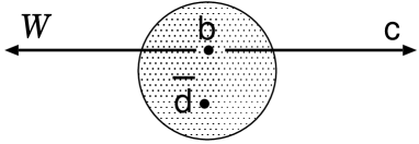
Figure 1: $B\rightarrow D^{(*)}$ transition through the $b$ quark decay into a $c$ quark and a virtual $W$ boson.

Write the $B$ ($D^{(*)}$) meson momentum $P_{1}$ ($P_{2}$) in the light-cone coordinates as

$$P_{1}=\frac{m_{B}}{\sqrt{2}}(1,1,{\bf 0}_{T})\;,\;\;\;\;P_{2}=\frac{m_{B}}{\sqrt{2}}\left(1,\frac{m_{D^{(*)}}^{2}}{m_{B}^{2}},{\bf 0}_{T}\right)\;.$$ (2)

The picture associated with the $B\rightarrow D^{(*)}$ transition is shown in Fig. 1, where the initial state is approximated by the $b\bar{d}$ component. The $b$ quark decays into a $c$ quark and a virtual $W$ boson, which carries the momentum $q$. Since the constituents are roughly on the mass shell, we have the invariant masses $k_{i}^{2}\sim O(\bar{\Lambda}^{2})$, $i=1$ and 2, where $k_{1}$ ($k_{2}$) is the momentum of the spectator $\bar{d}$ quark in the $B$ ($D^{(*)}$) meson. The above kinematic constraints lead to the order of magnitude of $k_{1}$ and $k_{2}$ [20],

$$k_{1}^{\mu} \sim (\bar{\Lambda},\bar{\Lambda},\bar{\Lambda})\;,$$

$$k_{2}^{\mu} \sim \left(\frac{m_{B}}{m_{D^{(*)}}}\bar{\Lambda},\frac{m_{D^{(*)}}}{m_{B}}\bar{\Lambda},\bar{\Lambda}\right)\;.$$ (3)

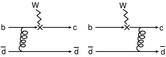
Figure 2: Lowest-order diagrams contributing to the $B\rightarrow D^{(*)}$ form factors. Quite a bit of momentum must be transfered to the spectator $\bar{d}$ quark through the hard gluon exchange.

The lowest-order diagrams contributing to the $B\rightarrow D^{(*)}$ form factors contain a hard gluon exchange between the $b$ or $c$ quark and the $\bar{d}$ quark as shown in Fig. 2. The $\bar{d}$ quark undergoes scattering in order to catch up with the $c$ quark, forming a $D^{(*)}$ meson. With the parton momenta in Eq. (3), the exchanged gluon is off-shell by

$$(k_{1}-k_{2})^{2}\sim-\frac{m_{B}}{m_{D^{(*)}}}\bar{\Lambda}^{2}\;,$$ (4)

which has been identified as the characteristic scale of the hard kernels. Under Eq. (1), we have $m_{B}/m_{D}^{(*)}\gg 1$, and the hard kernels are calculable in perturbation theory. It has been found that the applicability of PQCD to the $B\rightarrow D^{(*)}$ transition at large recoil is marginal for the physical masses $m_{B}$ and $m_{D^{(*)}}$ [20].

Infrared divergences arise from higher-order corrections to Fig. 2. The soft (collinear) type of divergences is absorbed into the $B$ ($D^{(*)}$) meson wave function $\phi_{B}(x_{1},b_{1})$ ($\phi_{D^{(*)}}(x_{2},b_{2})$), which is not calculable but universal. The impact parameter $b_{1}$ ($b_{2}$) is conjugate to the transverse momentum $k_{1T}$ ($k_{2T}$) carried by the $\bar{d}$ quark in the $B$ ($D^{(*)}$) meson. It has been shown, from equations of motion for the relevant nonlocal matrix elements, that $\phi_{B}(x_{1},b_{1})$ ($\phi_{D^{(*)}}(x_{2},b_{2})$) has a peak at the momentum fraction $x_{1}\equiv k_{1}^{-}/P_{1}^{-}\sim\bar{\Lambda}/m_{B}$ ($x_{2}\equiv k_{2}^{+}/P_{2}^{+}\sim\bar{\Lambda}/m_{D^{(*)}}$) [20].

The form factors are then expressed as the convolution of the hard kernels $H$ with the $B$ and $D^{(*)}$ meson wave functions in $k_{T}$ factorization theorem,

$$F^{BD^{(*)}}(q^{2})=\int dx_{1}dx_{2}d^{2}b_{1}d^{2}b_{2}\phi_{B}(x_{1},b_{1})H(x_{1},x_{2},b_{1},b_{2})\phi_{D^{(*)}}(x_{2},b_{2})\;.$$ (5)

The $D^{(*)}$ meson wave function contains a Sudakov factor arising from $k_{T}$ resummation, which sums the large double logarithms $\alpha_{s}\ln^{2}(m_{B}b_{2})$ to all orders. The $B$ meson wave function also contains such a Sudakov factor, whose effect is negligible because a $B$ meson is dominated by soft dynamics. The hard kernels involve a Sudakov factor from threshold resummation, which sums the large double logarithm $\alpha_{s}\ln^{2}x_{1}$ or $\alpha_{s}\ln^{2}x_{2}$ to all orders. This factor modifies the end-point behavior of the $B$ and $D^{(*)}$ meson wave functions effectively, rendering them diminish faster in the small $x_{1,2}$ region.

2.2 End-point Singularity and Sudakov Factor

It has been pointed out that if evaluating Fig. 2 in collinear factorization theorem, an end-point singularity appears [21]. In this theorem we have the lowest-order hard kernel,

$$H^{(0)}(x_{1},x_{2})\propto\frac{1}{x_{1}x_{2}^{2}}\;,$$ (6)

from the left diagram in Fig. 2, which leads to a logarithmic divergence, as the $D^{(*)}$ meson distribution amplitude behaves like $\phi_{D^{(*)}}(x_{2})\propto x_{2}$ in the small $x_{2}$ region. This singularity implies the breakdown of collinear factorization, and $k_{T}$ factorization becomes more appropriate. Once the parton transverse momenta $k_{T}$ are taken into account, Eq. (6) is modified into

$$H^{(0)}(x_{1},x_{2},{\bf k}_{1T},{\bf k}_{2T})\propto\frac{m_{B}^{4}}{[x_{1}x_{2}m_{B}^{2}+({\bf k}_{1T}-{\bf k}_{2T})^{2}][x_{2}m_{B}^{2}+{\bf k}_{2T}^{2}]}\;.$$ (7)

A dynamical effect, the so-called Sudakov suppression, favors the configuration in which $k_{T}$ is not small [8]. The end-point singularity then disappears as explained below.

Figure 3: QCD demands the presence of a Sudakov factor, which is an amplitude for a quark-antiquark color dipole not to emit real gluons in the final state. For a large transverse separation $b$, the quark and the antiquark do not shield each other’s color charge, and intend to radiate. In this region Sudakov suppression is strong.

When an electron undergoes harder scattering, it intends to radiate more photons. Hence, the scattering amplitude for radiating no photons must be suppressed by a factor, whose effect increases with the electron energy. In QED it is the well-known Sudakov suppression factor, an amplitude for an electron not to emit a photon in hard scattering. In the current QCD case of the $B\rightarrow D^{(*)}$ transition, it is the $c$-$\bar{d}$ quark-antiquark color dipole that undergoes hard scattering. When the color dipole is larger, in intends to radiate more gluons. Since the final state contains only a single $D^{(*)}$ meson, the real gluon emission is forbidden in the hard decay process. Similarly, the transition amplitude must involve a Sudakov factor, whose effect increases with the size of the color dipole, i.e., with the separation $b$ between $c$ and $\bar{d}$. That is, the configuration with a smaller separation $b$ or with a larger relative transverse momentum $k_{T}$ is preferred in the $B\rightarrow D^{(*)}$ transition at large recoil. Then the virtual particles involved in the hard kernel remain sufficiently off-shell, and Eq. (5), with Eq. (7) inserted, is free from the end-point singularity.

The corresponding Sudakov factor can be derived in PQCD as a function of the transverse separation $b$ and of the momentum fraction $x$ carried by the spectator quark [9], whose behavior is shown in Fig. 3. The Sudakov factor suppresses the large $b$ region, where the quark and the antiquark are separated by a large transverse distance and the color shielding is not effective. It also suppresses the $x\sim 1$ region, where a quark carries all of the meson momentum, and intends to emit real gluons in hard scattering. The Sudakov factors from $k_{T}$ resummation [22] for the $B$ and $D^{(*)}$ mesons are only associated with the light spectator quarks, since the double logarithms arise from the overlap of the soft and mass (collinear) divergences. These factors, being universal, are the same as in all our previous analyses.

Similarly, the small $x$ region corresponds to a configuration with a soft spectator, i.e., with a large color dipole in the longitudinal direction. The probability for this large color dipole not to radiate in hard scattering is also described by a Sudakov factor, which comes from threshold resummation for the hard kernels. For the derivation of this Sudakov factor, refer to [23]. For convenience, it has been parametrized as [24],

$$S_{t}(x)=\frac{2^{1+2c}\Gamma(3/2+c)}{\sqrt{\pi}\Gamma(1+c)}[x(1-x)]^{c}\;,$$ (8)

with the constant $c=0.35$. The above parametrization is motivated by the qualitative behavior of $S_{t}$: $S_{t}(x)\rightarrow 0$ as $x\rightarrow 0$, 1 [23]. Since threshold resummation is associated with the hard kernels, the result could be process-dependent. It has been observed [25] that its effect is essential for factorizable decay topologies, and negligible for nonfactorizable decay topologies.

2.3 Factorization Assumption

We review the basics of FA for the $B\rightarrow D^{(*)}M$ decays. The relevant effective weak Hamiltonian is given by

$${\cal H}_{\rm eff}={G_{F}\over\sqrt{2}}\,V_{cb}V_{ud}^{*}\Big{[}C_{1}(\mu)O_{1}(\mu)+C_{2}(\mu)O_{2}(\mu)\Big{]}\;,$$ (9)

where the four-fermion operators are

$$O_{1}=(\bar{d}b)_{V-A}(\bar{c}u)_{V-A}\;,\qquad\qquad O_{2}=(\bar{c}b)_{V-A}(\bar{d}u)_{V-A}\;,$$ (10)

with the definition $(\bar{q}_{1}q_{2})_{V-A}\equiv\bar{q}_{1}\gamma_{\mu}(1-\gamma_{5})q_{2}$, $V$’s the Cabibbo-Kobayashi-Maskawa (CKM) matrix elements, and $C_{1}$ and $C_{2}$ the Wilson coefficients. The $\bar{B}^{0}\rightarrow D^{+}\pi^{-}$ mode is referred to as the class-1 (color-allowed) topology, in which the charged pion is emitted at the weak vertex. The $\bar{B}^{0}\rightarrow D^{0}\pi^{0}$ mode is referred to as the class-2 (color-suppressed) topology, in which the $D^{0}$ meson is directly produced.

For the $\bar{B}^{0}\rightarrow D^{+}\pi^{-}$ mode, $O_{2}$ and Fierz transformed $O_{1}$ contribute. For the $\bar{B}^{0}\rightarrow D^{0}\pi^{0}$ mode, $O_{1}$ and Fierz transformed $O_{2}$ contribute. Applying FA [1] or generalized FA [2, 3, 4] to the hadronic matrix elements, we have

$$\langle D^{+}\pi^{-}|(\bar{c}b)_{V-A}(\bar{d}u)_{V-A}|\bar{B}^{0}\rangle\approx\langle D^{+}|(\bar{c}b)_{V-A}|\bar{B}^{0}\rangle\langle\pi^{-}|(\bar{d}u)_{V-A}|0\rangle\;,$$

$$\langle D^{0}\pi^{0}|(\bar{d}b)_{V-A}(\bar{c}u)_{V-A}|\bar{B}^{0}\rangle\approx\langle\pi^{0}|(\bar{d}b)_{V-A}|\bar{B}^{0}\rangle\langle D^{0}|(\bar{c}u)_{V-A}|0\rangle\;.$$ (11)

Substituting the definition of the $B$ meson transition form factors, $F^{BD}$ and $F^{B\pi}$, and of the meson decay constants, $f_{\pi}$ and $f_{D}$, the $\bar{B}^{0}\rightarrow D^{+}\pi^{-}$ (class-1) and $\bar{B}^{0}\rightarrow D^{0}\pi^{0}$ (class-2) decay amplitudes are expressed as

$$A(\bar{B}^{0}\rightarrow D^{+}\pi^{-}) = i\,\frac{G_{F}}{\sqrt{2}}\,V_{cb}V_{ud}^{*}\,(m_{B}^{2}-m_{D}^{2})\,f_{\pi}\,F^{BD}(m_{\pi}^{2})\,a_{1}(D\pi)\;,$$ (12)

$$\sqrt{2}\,A(\bar{B}^{0}\rightarrow D^{0}\pi^{0}) = -i\,\frac{G_{F}}{\sqrt{2}}\,V_{cb}V_{ud}^{*}\,(m_{B}^{2}-m_{\pi}^{2})\,f_{D}\,F^{B\pi}(m_{D}^{2})\,a_{2}(D\pi)\;,$$ (13)

where the parameters $a_{1}$ and $a_{2}$ are defined by

$$a_{1}=C_{2}(\mu)+{C_{1}(\mu)\over N_{c}}\;,\;\;\;\;a_{2} = C_{1}(\mu)+{C_{2}(\mu)\over N_{c}}\;,$$ (14)

$N_{c}$ being the number of colors. The $B^{-}\rightarrow D^{0}\pi^{-}$ mode, involving both classes of amplitudes, is referred to as class-3. The isospin symmetry implies

$$A(\bar{B}^{0}\rightarrow D^{+}\pi^{-})=A(B^{-}\rightarrow D^{0}\pi^{-})+\sqrt{2}\,A(\bar{B}^{0}\rightarrow D^{0}\pi^{0})\;.$$ (15)

It is straightforward to apply FA to other $\bar{B}\rightarrow D^{(*)}M$ modes. $a_{1}$ and $a_{2}$ depend on the color and Dirac structures of the operators, but otherwise are postulated to be universal [1, 26, 27]. They have the orders of magnitude $a_{1}(D\pi)\sim O(1)$ and $a_{2}(D\pi)\sim O(1/N_{c})$. The consistency of FA can be tested by comparing $a_{1}$ and $a_{2}$ extracted from various decays. Within errors, the class-1 decays $\bar{B}^{0}\rightarrow D^{(*)+}M^{-}$ with $M=\pi,\rho,a_{1},D_{s}$, and $D_{s}^{*}$ are described using a universal value $|a_{1}|\approx 1.1\pm 0.1$, whereas the class-2 decays $\bar{B}\rightarrow\bar{K}^{(*)}M$ with $M=J/\psi$ and $\psi(2S)$ suggest a nearly universal value $|a_{2}|\approx 0.2$–0.3 [28]. The wide range of $|a_{2}|$ is due to the uncertainty in the $B\rightarrow K^{(*)}$ form factors. The class-3 decays $B^{-}\rightarrow D^{(*)0}M^{-}$ with $M=\pi$ and $\rho$, which are sensitive to the interference of the two decay topologies, can be explained by a real and positive ratio $a_{2}/a_{1}\approx 0.2$–0.3, which seemed to agree with the above determination of $|a_{1}|$ and $|a_{2}|$. This is the reason FA was claimed to work well in explaining two-body charmed $B$ meson decays, before the class-2 modes $\bar{B}^{0}\rightarrow D^{0}M^{0}$ with $M=\pi,\eta$, and $\omega$ were measured.

The recently observed $\bar{B}^{0}\rightarrow D^{0}M^{0}$ branching ratios listed in Table 1 [29, 30] revealed interesting QCD dynamics. The parameter $|a_{2}|$ directly extracted from these modes falls into the range of $|a_{2}(D\pi)|\sim 0.35-0.60$ and $|a_{2}(D^{*}\pi)|\sim 0.25-0.50$ [31]. To maintain the predictions for the class-3 decays, there must exist sizeable relative strong phases between class-1 and class-2 amplitudes [19], which are $Arg(a_{2}/a_{1})=59^{\circ}$ for the $D\pi$ modes and $Arg(a_{2}/a_{1})=63^{\circ}$ for the $D^{*}\pi$ modes [31]. These results can be regarded as a failure of FA: the parameters $a_{2}$ in different types of decays, such as $\bar{B}\rightarrow D^{(*)}\pi$ and $\bar{B}\rightarrow\bar{K}^{(*)}J/\psi$, differ by almost a factor 2 in magnitude, implying strong nonuniversal nonfactorizable effects. It is then crucial to understand this nonuniversality and, especially, the mechanism responsible for the large relative phases in a systematic QCD framework.

3 $B\rightarrow D\pi$ IN PQCD

In this section we take the $B\rightarrow D\pi$ decays as an example of the PQCD analysis. The intensive study of all other modes will be performed in the next section. The $B\rightarrow D\pi$ decay rates have the expressions,

$$\Gamma_{i}=\frac{1}{128\pi}G_{F}^{2}|V_{cb}|^{2}|V_{ud}|^{2}\frac{m_{B}^{3}}{r}|A_{i}|^{2}\;.$$ (16)

The indices for the classes $i=1$, 2, and 3, denote the modes ${\bar{B}}^{0}\rightarrow D^{+}\pi^{-}$, ${\bar{B}}^{0}\rightarrow D^{0}\pi^{0}$, and $B^{-}\rightarrow D^{0}\pi^{-}$, respectively. The amplitudes $A_{i}$ are written as

$$A_{1} = f_{\pi}\xi_{\rm ext}+f_{B}\xi_{\rm exc}+{\cal M}_{\rm ext}+{\cal M}_{\rm exc}\;,$$ (17)

$$\sqrt{2}A_{2} = -(f_{D}\xi_{\rm int}-f_{B}\xi_{\rm exc}+{\cal M}_{\rm int}-{\cal M}_{\rm exc})\;,$$ (18)

$$A_{3} = f_{\pi}\xi_{\rm ext}+f_{D}\xi_{\rm int}+{\cal M}_{\rm ext}+{\cal M}_{\rm int}\;,$$ (19)

with $f_{B}$ being the $B$ meson decay constant. The functions $\xi_{\rm ext}$, $\xi_{\rm int}$, and $\xi_{\rm exc}$ denote the factorizable external $W$-emission (color-allowed), internal $W$-emission (color-suppressed), and $W$-exchange contributions, which come from Figs. 4(a) and 4(b), Figs. 5(a) and 5(b), and Figs. 6(a) and 6(b), respectively. The functions ${\cal M}_{\rm ext}$, ${\cal M}_{\rm int}$, and ${\cal M}_{\rm exc}$ represent the nonfactorizable external $W$-emission, internal $W$-emission, and $W$-exchange contributions, which come from Figs. 4(c) and 4(d), Figs. 5(c) and 5(d), and Figs. 6(c) and 6(d), respectively. All the topologies, including the factorizable and nonfactorizable ones, have been taken into account. It is easy to find that Eqs. (17)-(19) obey the isospin relation in Eq. (15).

Figure 4: Color-allowed emission diagrams contributing to the $B\rightarrow D^{(*)}\pi$ decays.

Figure 5: Color-suppressed emission diagrams contributing to the $B\rightarrow D^{(*)}\pi$ decays.

Figure 6: Annihilation Diagrams contributing to the $B\rightarrow D^{(*)}\pi$ decays.

In the PQCD framework based on $k_{T}$ factorization theorem, an amplitude is expressed as the convolution of hard $b$ quark decay kernels with meson wave functions in both the longitudinal momentum fractions and the transverse momenta of partons. Our PQCD formulas are derived up to leading-order in $\alpha_{s}$, to leading power in $m_{D}/m_{B}$ and in $\bar{\Lambda}/m_{D}$, and to leading double-logarithm resummations. For the Wilson coefficients, we adopt the leading-order renormalization-group evolution for consistency, although the next-to-leading-order ones are available in the literature [32]. For the similar reason, we employ the one-loop running coupling constant $\alpha_{s}(\mu)=2\pi/[\beta_{1}\ln(\mu/{\Lambda_{\rm QCD}^{(n_{f})}})]$ with $\beta_{1}=(33-2n_{f})/3$, $n_{f}$ being the number of active quarks. The QCD scale is chosen as $\Lambda_{\rm QCD}^{(5)}=193$ MeV for the scale $m_{b}<\mu<m_{W}$, which is derived from $\Lambda_{\rm QCD}^{(4)}=250$ MeV for $\mu<m_{b}$.

The leading-order and leading-power factorization formulas for the above decay amplitudes are collected in Appendix A. Here we mention only some key ingredients in the calculation. The formulas for the $B\rightarrow D\pi$ decays turn out to be simpler than those for the $B\rightarrow\pi\pi$ ones. The simplicity is attributed to the power counting rules under the hierachy of the three scales in Eq. (1). The hard kernels are evaluated up to the power corrections of order $\bar{\Lambda}/m_{D}\sim m_{D}/m_{B}$ ($\bar{\Lambda}/m_{B}$ is regarded as being of even higher power). Following these rules, the terms proportional to $x_{1}\sim\bar{\Lambda}/m_{B}$ and to $x_{2}\sim\bar{\Lambda}/m_{D}$ are higher-power compared to the leading $O(1)$ terms and dropped. We have also dropped the terms of higher powers in $r=m_{D}/m_{B}$. Accordingly, the phase space factor $1-r^{2}$, appearing in Eq. (16) originally, has been approximated by 1. This approximation is irrelevant for explaining the ratios of the $B\rightarrow D\pi$ branching ratios, and causes an uncertainty in the absolute branching ratios, which is much smaller than those from the CKM matrix element $|V_{cb}|$, and from the meson decay constants $f_{B}$ and $f_{D}$.

Up to the power corrections of order $\bar{\Lambda}/m_{B}$ and $\bar{\Lambda}/m_{D}$, we consider only a single $B$ ($D$) meson wave function. The nonperturbative $B$ meson and pion wave functions have been fixed in our previous works [14, 15]. The unknown $D$ meson wave function was determined by fitting the PQCD predictions for the $B\rightarrow D$ transition form factors to the observed $B\rightarrow Dl\nu$ decay spectrum [20]. The contributions from the two-parton twist-3 $D$ meson wave functions, being higher-power, are negligible. Note that in the charmless decays the contributions from the two-parton twist-3 light meson distribution amplitudes are not down by a power of $1/m_{B}$. These distribution amplitudes, being constant at the momentum fraction $x\rightarrow 0$ as required by equations of motion, lead to linear singularities in the collinear factorization formulas. The linear singularities modify the naive power counting, such that two-parton twist-3 contributions become leading-power [24, 33]. In the charmed decays the above equations of motion are modified [20], and the two-parton twist-3 $D$ meson wave functions vanish at the end point of $x$. Therefore, their contributions are indeed higher-power.

Retaining the parton transverse momenta $k_{T}$, the nonfactorizable topologies generate strong phases from non-pinched singularities of the hard kernels [34]. For example, the virtual quark propagator in Fig. 5(d) is written, in the principle-value prescription, as

$$\frac{1}{x_{3}(x_{2}-x_{1})m_{B}^{2}-({\bf k}_{2T}-{\bf k}_{1T}+{\bf k}_{3T})^{2}+i\epsilon} = P\left[\frac{1}{x_{3}(x_{2}-x_{1})m_{B}^{2}-({\bf k}_{2T}-{\bf k}_{1T}+{\bf k}_{3T})^{2}}\right]$$

$$-i\pi\delta(x_{3}(x_{2}-x_{1})m_{B}^{2}-({\bf k}_{2T}-{\bf k}_{1T}+{\bf k}_{3T})^{2})\;,$$

with $x_{3}$ being the momentum fraction associated with the pion. The second term contributes to the strong phase, which is thus of short-distance origin and calculable. The first term in the above expression does not lead to an end-point singularity. Note that the strong phase from Eq. (LABEL:pri) is obtained by keeping all terms in the denominator of a propagator without neglecting $x_{1}$ and $x_{2}$.

4 NUMERICAL RESULTS

The computation of the hard kernels in $k_{T}$ factorization theorem for other charmed decay modes is similar and straightforward. The $B\rightarrow D^{*}\pi$ decay amplitudes are the same as the $B\rightarrow D\pi$ ones but with the substitution of the mass, the decay constant, and the distribution amplitude,

$$m_{D}\rightarrow m_{D^{*}}\;,\;\;f_{D}\rightarrow f_{D^{*}}\;,\;\;\phi_{D}(x_{2})\rightarrow\phi_{D^{*}}(x_{2})\;.$$ (21)

This simple substitution is expected at leading power under the hierachy in Eq. (1): the difference between the two channels should occur only at $O(\bar{\Lambda}/m_{D})$. An explicit derivation shows that the difference occurs at the twist-3 level for the nonfactorizable emission diagrams in Fig. 4 and for the annihilation diagrams in Fig. 6. It implies that the universality (channel-independence) of $a_{1}$ and $a_{2}$ assumed in FA [35] breaks down at subleading power even within the $B\rightarrow D^{(*)}M$ decays.

Replacing the pion in Figs. 4-6 by the $\rho$ ($\omega$) meson, we obtain the diagrams for the $B\rightarrow D^{(*)}\rho(\omega)$ decays. The factorization formulas for the $B\rightarrow D\rho(\omega)$ decay amplitudes are also the same as those for the $B\rightarrow D\pi$ ones but with the substitution,

$$\phi_{\pi}\rightarrow\phi_{\rho,\omega}\;,\;\;\;\;\phi_{\pi}^{p}\rightarrow\phi_{\rho,\omega}^{s}\;,\;\;\;\;\phi_{\pi}^{t}\rightarrow\phi_{\rho,\omega}^{t}\;,\;\;\;\;m_{0}\rightarrow m_{\rho(\omega)}\;,$$ (22)

where $\phi_{\pi}$ ($\phi_{\pi}^{p,t}$) is the two-parton twist-2 (twist-3) pion distribution amplitude, $\phi_{\rho,\omega}$ ($\phi_{\rho,\omega}^{s,t}$) the two-parton twist-2 (twist-3) $\rho$ and $\omega$ meson distribution amplitudes, respectively, $m_{0}$ the chiral enhancement scale, and $m_{\rho(\omega)}$ the $\rho$ ($\omega$) meson mass. Hence, the similar isospin relation holds:

$$A(B^{0}\rightarrow D^{-}\rho^{+})=A(B^{+}\rightarrow\bar{D}^{0}\rho^{+})+\sqrt{2}A(B^{0}\rightarrow\bar{D}^{0}\rho^{0})\;.$$ (23)

The $B\rightarrow D^{*}\rho(\omega)$ decays contain more amplitudes associated with the different polarizations. However, at leading power, the amplitudes associated with the transverse polarizations, suppressed by a power of $m_{D^{*}}/m_{B}$ or of $m_{\rho}/m_{B}$, are negligible. That is, the factorization formulas for the $B\rightarrow D^{*}\rho(\omega)$ modes are the same as the $B\rightarrow D\rho(\omega)$ ones with the substitution in Eq. (21). Note that the $W$-exchange contribution changes sign in the $\bar{B}^{0}\rightarrow D^{(*)0}\omega$ decay amplitude:

$$A(\bar{B}^{0}\rightarrow D^{(*)0}\omega)=-\frac{1}{\sqrt{2}}(f_{D^{(*)}}\xi_{\rm int}+f_{B}\xi_{\rm exc}+{\cal M}_{\rm int}+{\cal M}_{\rm exc})\;,$$ (24)

due to the different quark structures between the $\omega$ meson (proportional to $u\bar{u}+d\bar{d}$) and the $\rho^{0}$ meson (proportional to $u\bar{u}-d\bar{d}$).

In the numerical analysis we adopt the model for the $B$ meson wave function,

$$\phi_{B}(x,b)=N_{B}x^{2}(1-x)^{2}\exp\left[-\frac{1}{2}\left(\frac{xm_{B}}{\omega_{B}}\right)^{2}-\frac{\omega_{B}^{2}b^{2}}{2}\right]\;,$$ (25)

with the shape parameter $\omega_{B}$ and the normalization constant $N_{B}$ being related to the decay constant $f_{B}$ through

$$\int dx\phi_{B}(x,0)=\frac{f_{B}}{2\sqrt{2N_{c}}}\;.$$ (26)

The $D^{(*)}$ meson distribution amplitude is given by

$$\phi_{D^{(*)}}(x)=\frac{3}{\sqrt{2N_{c}}}f_{D^{(*)}}x(1-x)[1+C_{D^{(*)}}(1-2x)]\;,$$ (27)

with the shape parameter $C_{D^{(*)}}$. The pion and $\rho(\omega)$ meson distribution amplitudes have been derived in [36, 37], whose explicit expressions are given in Appendix A. The $B$ meson wave function was then extracted from the light-cone-sum-rule (LCSR) results of the $B\rightarrow\pi$ transition form factor [24]. The range of $C_{D^{(*)}}$ was determined from the measured $B\rightarrow D^{(*)}l\nu$ decay spectrum at large recoil employing the $B$ meson wave function extracted above. We do not consider the variation of $\phi_{D^{(*)}}$ with the impact parameter $b$, since the available data are not yet sufficiently precise to control this dependence.

The input parameters are listed below:

$$f_{B}=190\;{\rm MeV}\;,\;\;\omega_{B}=0.4\;{\rm GeV}\;,$$

$$f_{D}=240\;{\rm MeV}\;,\;\;C_{D}=0.8\pm 0.2\;,$$

$$f_{D^{*}}=230\;{\rm MeV}\;,C_{D^{*}}=0.7\pm 0.2\;,$$

$$f_{\pi}=132\;{\rm MeV}\;,\;\;f_{\rho}=f_{\omega}=200\;{\rm MeV}\;,\;\;f_{\rho}^{T}=f_{\omega}^{T}=160\;{\rm MeV}\;,$$

$$m_{B}=5.28\;{\rm GeV}\;,\;\;m_{b}=4.8\;{\rm GeV}\;,\;\;$$

$$m_{D}=1.87\;{\rm GeV}\;,\;\;m_{D^{*}}=2.01\;{\rm GeV}\;,\;\;m_{c}=1.3\;{\rm GeV}\;,\;\;$$

$$m_{\rho}=0.77\;{\rm GeV}\;,\;\;m_{\omega}=0.78\;{\rm GeV}\;,$$

$$m_{t}=170\;{\rm GeV}\;,\;\;m_{W}=80.41\;{\rm GeV}\;,\;\;m_{0}=1.4\;{\rm GeV}\;,$$

$$\tau_{B^{\pm}}=1.674\times 10^{-12}{\rm s}\;,\;\;\tau_{B^{0}}=1.542\times 10^{-12}{\rm s}\;,$$

$$G_{F}=1.16639\times 10^{-5}\;{\rm GeV}^{-2}\;,\;\;|V_{cb}|=0.043\;,\;\;|V_{ud}|=0.974\;,$$ (28)

where $m_{t}$, $m_{W}$, $\tau_{B^{\pm}}$ and $\tau_{B^{0}}$ denote the top quark mass, the $W$ boson mass, the $B^{\pm}$ meson lifetime, and the $B^{0}$ meson lifetime, respectively. The above meson wave functions and parameters correspond to the form factors at maximal recoil,

$$F_{0}^{B\pi}\sim 0.3\;,~{}~{}~{}~{}~{}~{}\xi_{+}^{BD}\sim 0.57\;,~{}~{}~{}~{}~{}~{}\xi_{A_{1}}^{BD^{*}}\sim 0.52\;,$$ (29)

which are close to the results from QCD sum rules [38, 39]. We stress that there is no arbitrary parameter in our calculation, though the value of each parameter is only known up to a range.

The PQCD predictions for each term of the $B\rightarrow D\pi$ decay amplitudes are exhibited in Table 2. The theoretical uncertainty comes only from the variation of the shape parameter for the $D$ meson distribution amplitude, $0.6<C_{D}<1.0$. It is expected that the color-allowed factorizable amplitude $f_{\pi}\xi_{\rm ext}$ dominates, and that the color-suppressed factorizable contribution $f_{D}\xi_{\rm int}$ is smaller due to the Wilson coefficient $C_{1}+C_{2}/N_{c}\sim 0$. The color-allowed nonfactorizable amplitude ${\cal M}_{\rm ext}$ is negligible: since the pion distribution amplitude is symmetric under the exchange of $x_{3}$ and $1-x_{3}$, the contributions from the two diagrams Figs. 4(c) and 4(d) cancel each other in the dominant region with small $x_{2}$. It is also down by the small Wilson coefficient $C_{1}/N_{c}$. For the color-suppressed nonfactorizable contribution ${\cal M}_{\rm int}$, the above cancellation does not exist in the dominant region with small $x_{3}$, because the $D$ meson distribution amplitude $\phi_{D}(x_{2})$ is not symmetric under the exchange of $x_{2}$ and $1-x_{2}$. Furthermore, ${\cal M}_{\rm int}$, proportional to $C_{2}/N_{c}\sim 0.3$, is not down by the Wilson coefficient. It is indeed comparable to the color-allowed factorizable amplitude $f_{\pi}\xi_{\rm ext}$, and produces a large strong phase as explained in Eq. (LABEL:pri). Both the factorizable and nonfactorizable annihilation contributions are small, consistent with our argument in Sec. II.

The predicted branching ratios in Table 3 are in agreement with the averaged experimental data [29, 30, 40]. We extract the parameters $a_{1}$ and $a_{2}$ by equating Eqs. (12) and (13) to Eqs. (17) and (18), respectively. That is, our $a_{1}$ and $a_{2}$ do not only contain the nonfactorizable amplitudes as in generalized FA, but the small annihilation amplitudes, which was first discussed in [41]. We obtain the ratio $|a_{2}/a_{1}|\sim 0.43$ with $10\%$ uncertainty and the phase of $a_{2}$ relative to $a_{1}$ about $Arg(a_{2}/a_{1})\sim-42^{\circ}$. If excluding the annihilation amplitudes $f_{B}\xi_{\rm exc}$ and ${\cal M}_{\rm exc}$, we have $|a_{2}/a_{1}|\sim 0.46$ and $Arg(a_{2}/a_{1})\sim-64^{\circ}$. Note that the experimental data do not fix the sign of the relative phases. The PQCD calculation indicates that $Arg(a_{2}/a_{1})$ should be located in the fourth quadrant. It is evident that the short-distance strong phase from the color-suppressed nonfactorizable amplitude is already sufficient to account for the isospin triangle formed by the $B\rightarrow D\pi$ modes. The conclusion that the data hint large final-state interaction was drawn from the analysis based on FA [19, 31, 42, 43]. Hence, it is more reasonable to claim that the data just imply a large strong phase, but do not tell what mechanism generates this phase [44]. From the viewpoint of PQCD, this strong phase is of short distance, and produced from the non-pinched singularity of the hard kernel. Certainly, under the current experimental and theoretical uncertainties, there is still room for long-distance phases from final-state interaction.

The PQCD predictions for the $B\rightarrow D^{*}\pi$ decay amplitudes and branching ratios in Table 4 are also consistent with the data [45]. Since $m_{D^{*}}$ and $\phi_{D^{*}}$ are only slightly different from $m_{D}$ and $\phi_{D}$, respectively, the results are close to those in Table 3. The $B\rightarrow D^{*}\pi$ branching ratios are smaller than the $B\rightarrow D\pi$ ones because of the form factors $\xi^{BD^{*}}_{A_{1}}<\xi^{BD}_{+}$ as shown in Eq. (29). Similarly, the ratio $|a_{2}/a_{1}|$ and the relative phase $Arg(a_{2}/a_{1})$ are also close to those associated with the $B\rightarrow D\pi$ decays. We obtain the ratio $|a_{2}/a_{1}|\sim 0.47$ with $10\%$ uncertainty and the relative phase about $Arg(a_{2}/a_{1})\sim-41^{\circ}$. Excluding the annihilation amplitudes, we have $|a_{2}/a_{1}|\sim 0.5$ and $Arg(a_{2}/a_{1})\sim-63^{\circ}$.

The PQCD predictions for the $B\rightarrow D^{(*)}\rho(\omega)$ branching ratios are listed in Table 5, which match the data [45]. The $\bar{B}^{0}\rightarrow D^{+}\rho^{-}$ and $B^{-}\rightarrow D^{0}\rho^{-}$ branching ratios are about twice of the $\bar{B}^{0}\rightarrow D^{+}\pi^{-}$ and $B^{-}\rightarrow D^{0}\pi^{-}$ ones because of the larger $\rho$ meson decay constant, $(f_{\rho}/f_{\pi})^{2}\sim 2$. The relatively smaller $\bar{B}^{0}\rightarrow D^{0}\rho^{0}$ branching ratio is attributed to the cancellation of the above enhancing effect between the color-suppressed and $W$-exchange contributions, consistent with the observation made in an analysis based on the topological-amplitude parametrization [46]. The $\bar{B}^{0}\rightarrow D^{0}\omega$ branching ratio is larger than the $\bar{B}^{0}\rightarrow D^{0}\rho^{0}$ one due to the constructive inteference between the color-suppressed contribution and the annihilation contribution as indicated in Eq. (24). To obtain the ${\bar{B}}^{0}\rightarrow D^{*}\rho$ helicity amplitudes and their relative phases [47], the power-suppressed contributions from the transverse polarizations must be included. For consistency, the contribution from the longitudinal polarization should be calculated up to the same power. We shall study this subject in a forthcoming paper. The predictions for the $B\rightarrow D^{*0}\rho^{0}$, $D^{*0}\omega$ decays can be compared with future measurement. The latter branching ratio is larger than the former one because of the same reason as for the $B\rightarrow D^{0}\rho^{0}$, $D^{0}\omega$ decays.

5 COMPARISON WITH OTHER APPROACHES

In this section we make a brief comparison of the PQCD formalism with other QCD approaches to exclusive $B$ meson decays, emphasizing the differences. For more details, refer to [48]. As mentioned before, there are two kinds of factorization theorem for QCD processes [13]: collinear factorization, on which the soft-collinear effective theory (SCET) [49, 50], LCSR [51, 52], and QCDF [5] are based, and $k_{T}$ factorization, on which the PQCD approach is based. Calculating the $B\rightarrow\pi$ form factor $F^{B\pi}$ in collinear factorization up to leading power in $1/m_{B}$ and leading-order in $\alpha_{s}$, an end-point singularity occurs. Hence, we define three types of contributions: a genuine soft contribution $f^{\rm S}$, a contribution $f^{\rm EP}$ containing the end-point singularity, and a finite contribution $f^{\rm F}$:

$$F^{B\pi}=f^{\rm S}+f^{\rm EP}+f^{\rm F}\;.$$ (30)

The second term can not cover the complete soft contribution, because it is from a leading formalism. Note that the end-point singularity exists even in the heavy quark limit. Hence, $B$ meson decays differ from other exclusive processes, which become calculable in collinear factorization at sufficiently large momentum transfer.

There are two options to handle the above end-point singularity [53]: first, an end-point singularity in collinear factorization implies that exclusive $B$ meson decays are dominated by soft dynamics. Therefore, a heavy-to-light form factor is not calculable, and $f^{\rm EP}$ should be treated as a soft object, like $f^{\rm S}$. In SCET and QCDF, $F^{B\pi}$ is then written, up to $O(\alpha_{s})$, as [54, 55]

$$F^{B\pi}=f^{\rm NF}+f^{\rm F}\;,$$ (31)

with

$$f^{\rm NF} = f^{\rm S}+f^{\rm EP}\;,$$

$$f^{\rm F} = \phi_{B}\otimes T^{\prime}\otimes\phi_{\pi}\;.$$ (32)

The soft form factor $f^{\rm NF}$, obeying the large-energy symmetry relations [56], can be estimated in terms of a triangle diagram without a hard gluon exchange in LCSR [38, 57]. However, since the pion vertex has been replaced by the pion distribution amplitudes under twist expansion, what is calculated in LCSR is not the full soft contribution. The term $f^{\rm F}$ has been expressed as a convolution of the hard-scattering kernel $T^{\prime}$ with the light-cone distribution amplitudes of the $B$ meson and of the pion in the momentum fractions, implying that it is calculable in collinear factorization.

The second option is that an end-point singularity indicates the breakdown of the collinear factorization. Hence, the $k_{T}$ factorization is the more appropriate framework, in which the parton transverse momenta $k_{T}$ are retained in the hard kernel, and $f^{\rm EP}$ does not develop an end-point singularity. Both $f^{\rm EP}$ and $f^{\rm F}$ are then calculable, and expressed, in the PQCD approach, as

$$F^{B\pi}=f^{\rm EP}+f^{\rm F}=\phi_{B}\otimes T\otimes\phi_{\pi}\;,$$ (33)

where the symbol $\otimes$ represents the convolution not only in the momentum fractions, but in the transverse separations. The hard kernel $T^{\prime}$ in Eq. (32) is derived from the complete hard kernel $T$ by dropping the terms which lead to the end-point singularity in the collinear factorization. Certainly, the subtraction of these terms depends on a regularization scheme [55]. The strong Sudakov suppression in the soft parton region implies that the genuine soft contribution $f^{\rm S}$ is not important [8, 24]. Equation (33) is then claimed to be a consequence of the hard-dominance picture, because a big portion of $F^{B\pi}$ is calculable. The agreement between the sum-rule and PQCD predictions for many $B$ meson transition form factors justifies that $f^{\rm S}$ is indeed negligible. Since $f^{\rm EP}$ remains in Eq. (33), the form factor symmetry relations at large recoil are still respected in the PQCD framework [24], which are then modified by the subleading term $f^{\rm F}$.

Therefore, the soft-dominance (hard-dominance) picture postulated in LCSR (PQCD) makes sense in the collinear ($k_{T}$) factorization [48]. The two pictures arise from the different theoretical frameworks, and there is no conflict at all. In other words, the soft contribution refers to $f^{\rm NF}$ in SCET, LCSR, and QCDF, which is large, but to $f^{\rm S}$ in PQCD, which is small. LCSR can be regarded as a method to evaluate $f^{\rm EP}$ or $f^{\rm NF}$ in the collinear factorization (at least the light-cone distribution amplitudes have been employed on the pion side), while the $k_{T}$ factorization is adopted in PQCD for the evaluation of $f^{\rm EP}$. We emphasize that there is no preference between the two options for semileptonic $B$ meson decays, both of which give similar results as stated above. However, in their extension to two-body nonleptonic $B$ meson decays, predictions could be very different. For example, the main source of strong phases in the $B\rightarrow\pi\pi$ decays is the correction to the weak vertex in QCDF, but the annihilation diagram in PQCD. This is the reason QCDF (PQCD) predicts a smaller and positive (larger and negative) CP asymmetry $C_{\pi\pi}$ [13, 58]. It is then possible to discriminate experimentally which theoretical framework works better.

Next we compare our formalism for two-body charmed nonleptonic $B$ meson decays based on the $k_{T}$ factorization with SCET and QCDF based on the collinear factorization. Currently, LCSR has not yet been applied to the nonfactorizable contribution discussed here, but only to that from three-parton distribution amplitudes [59], since the former, involving two loops, is more complicated to analyze. Similarly, the neglect of $k_{T}$ results in end-point singularities in the factorizable contributions $\xi_{\rm ext}$ and $\xi_{\rm int}$, which need to be parametrized in terms of the $B\rightarrow D$ and $B\rightarrow\pi$ transition form factors, respectively. It also causes an end-point singularity in the color-suppressed nonfactorizable amplitude ${\cal M}_{\rm int}$, if the $c$ quark is treated as being massive. This is why the color-suppressed modes, i.e., the magnitude and the phase of $a_{2}$, can not be predicted in QCDF, and the proof of QCDF in the SCET formalism [60] considered only the color-allowed mode $\bar{B}^{0}\rightarrow D^{+}\pi^{-}$. The color-allowed nonfactorizable amplitude ${\cal M}_{\rm ext}$ is calculable in QCDF, because the end-point singularities cancel between the pair of diagrams, Figs. 4(c) and 4(d). We mention a recent work on SCET [61], in which the color-suppressed nonfactorizable amplitude has been parametrized as an expression similar to Eq. (31).

If the $c$ quark is treated as being massless, the end-point singularities in the pair of color-suppressed nonfactorizable diagrams, Figs. 5(c) and 5(d), will cancel each other as in the charmless case [33, 58]. This can be understood by examining the behavior of the integrand of ${\cal M}_{\rm int}$ in Eq. (45) in the dominant region with small $x_{3}$, noticing that the $D$ meson distribution amplitude $\phi_{D}(x_{2})$ would be symmetric under the exchange of $x_{2}$ and $1-x_{2}$ in the $m_{c}\rightarrow 0$ limit. However, the nonfactorizable contribution will become negligible in this limit, such that the amplitude ${\cal M}_{\rm int}$, though calculable in QCDF, is not large enough to explain the $B\rightarrow D\pi$ data. It is then obvious that the PQCD approach has made a great contribution here: the nonfactorizable corrections to the naive factorizations of both the color-allowed and color-suppressed modes can be predicted, and the latter is found to be very important.

6 CONCLUSION

In this paper we have analyzed the two-body charmed nonleptonic decays $B\rightarrow D^{(*)}M$ with $M=\pi$, $\rho$, and $\omega$ in the PQCD approach. This framework is based on $k_{T}$ factorization theorem, which is free of end-point singularities and gauge-invariant. $k_{T}$ factorization theorem is more appropriate, when the end-point region of a momentum fraction is important, and collnear factorization theorem breaks down. By including the transverse degrees of freedom of partons in the evaluation of a hard kernel, and the Sudakov factors from $k_{T}$ and threshold resummations, the virtual particles remain sufficiently off-shell, and the end-point singularities do not exist. We have explained that there is no conflict between LCSR with the soft-dominance picture and PQCD with the hard-dominance picture, since the soft contributions refer to the different quantities in the two theoretical frameworks.

The derivation of the factorization formulas for the $B\rightarrow D^{(*)}M$ decay amplitudes follow the power counting rules constructed in our previous work on the $B\rightarrow D^{(*)}$ transition form factors. Under the hierachy $m_{B}\gg m_{D^{(*)}}\gg\bar{\Lambda}$, the $B$ and $D^{(*)}$ meson wave functions exhibit a peak at the momentum fractions around $\bar{\Lambda}/m_{B}$ and $\bar{\Lambda}/m_{D^{(*)}}$, respectively. Up to leading power in $m_{D^{(*)}}/m_{B}$ and in $\bar{\Lambda}/m_{D^{(*)}}$, only a single $B$ meson wave function and a single $D^{(*)}$ meson wave function are involved. The factorization formulas then become simpler than those for the charmless decays. Moreover, the factorization formulas for all the $B\rightarrow D^{(*)}M$ modes are identical, except the appropriate substitution of the masses, the decay constants, and the meson distribution amplitudes. We emphasize that there is no arbitrary parameter in our analysis (there are in QCDF), though all universal inputs are not yet known precisely. The meson wave functions have been determined either from the semileptonic data or from LCSR.

Being free from the end-point singularities, all topologies of decay amplitudes are calculable in PQCD, including the color-suppressed nonfactorizable one. This amplitude can not be computed in QCDF based on the collinear factorization theorem due to the existence of the end-point singularities for a massive $c$ quark. We have observed in PQCD that this amplitude, not suppressed by the Wilson coefficient (proportional to $C_{2}/N_{c}$), is comparable to the dominant color-allowed factorizable amplitude. It generates a large strong phase from the non-pinched singularity of the hard kernel, which is crucial for explaining the observed $B\rightarrow D^{(*)}M$ branching ratios. The other topologies are less important: the color-allowed nonfactorizable contribution is negligible because of the pair cancellation and the small Wilson coefficient $C_{1}/N_{c}$. The color-suppressed factorizable amplitude with the small Wilson coefficient $a_{2}=C_{1}+C_{2}/N_{c}$ is also negligible. The annihilation amplitudes are small, since they come from the tree operators.

All our predictions are consistent with the existing measurements. For those without data, such as the $B\rightarrow D^{*0}\rho^{0}$, $D^{*0}\omega$ modes, our predictions can be confronted with future measurement. As stated before, we have predicted the large strong phases from the scalar-penguin annihilation amplitudes, which are required by the large CP asymmetries observed in two-body charmless decays. The success in predicting the storng phases from the color-suppressed nonfactorizable amplitudes for the two-body charmed decays further supports the $k_{T}$ factorization theorem. The conclusion drawn in this work is that the short-distance strong phase is already sufficient to account for the $B\rightarrow D^{(*)}M$ data. Certainly, there is still room for long-distance strong phases from final-state interaction. For the application of the PQCD approach to other charmed decays, such as $B\rightarrow D_{s}^{(*)}K$ and $B\rightarrow D^{(*)}f_{0}$, refer to [62] and [63], respectively.

Appendix A FACTORIZATION FORMULAS FOR $B\rightarrow D\pi$

In this Appendix we present the factorization formulas for the $B\rightarrow D\pi$ decay amplitudes. We choose the $B$ meson, $D$ meson, and pion momenta in the light-cone coordinate as,

$$P_{1}=\frac{m_{B}}{\sqrt{2}}(1,1,{\bf 0}_{T})\;,\ \ P_{2}=\frac{m_{B}}{\sqrt{2}}(1,r^{2},{\bf 0}_{T})\;,\ \ P_{3}=\frac{m_{B}}{\sqrt{2}}(0,1-r^{2},{\bf 0}_{T})\;,$$ (34)

respectively, with $r=m_{D}/m_{B}$ being defined before. The fractional momenta of the light valence quarks in the $B$ meson, $D$ meson and the pion are

$$k_{1} = x_{1}\frac{m_{B}}{\sqrt{2}}(1,0,{\bf 0}_{T})+{\bf k}_{1T}\mbox{\ \ for\ \ $\xi_{\rm int}$, $M_{\rm int}$,}$$

$$k_{1} = x_{1}\frac{m_{B}}{\sqrt{2}}(0,1,{\bf 0}_{T})+{\bf k}_{1T}\mbox{\ \ for\ \ others,}$$

$$k_{2} = x_{2}\frac{m_{B}}{\sqrt{2}}(1,0,{\bf 0}_{T})+{\bf k}_{2T}\;,$$

$$k_{3} = x_{3}\frac{m_{B}}{\sqrt{2}}(0,1-r^{2},{\bf 0}_{T})+{\bf k}_{3T}\;,$$ (35)

respectively. Which longitudinal component of $k_{1}$, $k_{1}^{+}$ or $k_{1}^{-}$, is relevant depends on the final-state meson the hard gluon attaches. That is, it is selcted by the inner product $k_{1}\cdot k_{3}$ or $k_{1}\cdot k_{2}$.

The factorizable amplitudes $\xi_{\rm ext}$, $\xi_{\rm int}$ and $\xi_{\rm exc}$ are written as

$$\xi_{\rm ext} = 16\pi C_{F}\sqrt{r}m_{B}^{2}\int_{0}^{1}dx_{1}dx_{2}\int_{0}^{1/\Lambda}b_{1}db_{1}b_{2}db_{2}\phi_{B}(x_{1},b_{1})\phi_{D}(x_{2})$$ (36)

$$\times\left[E_{e}(t_{e}^{(1)})h(x_{1},x_{2},b_{1},b_{2})S_{t}(x_{2})+rE_{e}(t_{e}^{(2)})h(x_{2},x_{1},b_{2},b_{1})S_{t}(x_{1})\right]\;,$$

$$\xi_{\rm int} = 16\pi C_{F}\sqrt{r}m_{B}^{2}\int_{0}^{1}dx_{1}dx_{3}\int_{0}^{1/\Lambda}b_{1}db_{1}b_{3}db_{3}\phi_{B}(x_{1},b_{1})$$ (37)

$$\times\{[(1+x_{3})\phi_{\pi}(x_{3})+r_{0}(1-2x_{3})(\phi_{\pi}^{p}(x_{3})+\phi_{\pi}^{t}(x_{3}))]$$

$$\times E_{i}(t_{i}^{(1)})h(x_{1},x_{3}(1-r^{2}),b_{1},b_{3})S_{t}(x_{3})$$

$$\ \ +2r_{0}\phi_{\pi}^{p}(x_{3})E_{i}(t_{i}^{(2)})h(x_{3},x_{1}(1-r^{2}),b_{3},b_{1})S_{t}(x_{1})\}\;,$$

$$\ \xi_{\rm exc} = 16\pi C_{F}\sqrt{r}m_{B}^{2}\int_{0}^{1}dx_{2}dx_{3}\int_{0}^{1/\Lambda}b_{2}db_{2}b_{3}db_{3}\phi_{D}(x_{2})$$ (38)

$$\times\left[-x_{3}\phi_{\pi}(x_{3})E_{a}(t_{a}^{(1)})h_{a}(x_{2},x_{3}(1-r^{2}),b_{2},b_{3})S_{t}(x_{3})\right.$$

$$\ \ \ \left.+x_{2}\phi_{\pi}(x_{3})E_{a}(t_{a}^{(1)})h_{a}(x_{3},x_{2}(1-r^{2}),b_{3},b_{2})S_{t}(x_{2})\right]\;,$$

with the mass ratio $r_{0}\equiv m_{0}/m_{B}$, the evolution factors,

$$E_{e}(t) = \alpha_{s}(t)a_{1}(t)\exp[-S_{B}(t)-S_{D}(t)]\;,$$

$$E_{i}(t) = \alpha_{s}(t)a_{2}(t)\exp[-S_{B}(t)-S_{\pi}(t)]\;,$$

$$E_{a}(t) = \alpha_{s}(t)a_{2}(t)\exp[-S_{D}(t)-S_{\pi}(t)]\;,$$ (39)

and the Wilson coefficients,

$$a_{1}=C_{2}+\frac{C_{1}}{N_{c}}\;,\;\;\;\;a_{2}=C_{1}+\frac{C_{2}}{N_{c}}\;.$$ (40)

Note that $C_{1}=0$ and $C_{2}=1$ at tree level in our convention. The explicit expressions of the Sudakov factors $\exp[-S_{B}(t)]$, $\exp[-S_{D}(t)]$ and $\exp[-S_{\pi}(t)]$ from $k_{T}$ resummation are referred to [20, 24].

The functions $h$’s, obtained from Figs. 4(a) and 4(b), Figs. 5(a) and 5(b), and Figs. 6(a) and 6(b), are given by

$$h(x_{1},x_{2},b_{1},b_{2}) = K_{0}\left(\sqrt{x_{1}x_{2}}m_{B}b_{1}\right)$$ (41)

$$\times\left[\theta(b_{1}-b_{2})K_{0}\left(\sqrt{x_{2}}m_{B}b_{1}\right)I_{0}\left(\sqrt{x_{2}}m_{B}b_{2}\right)\right.$$

$$\left.+\theta(b_{2}-b_{1})K_{0}\left(\sqrt{x_{2}}m_{B}b_{2}\right)I_{0}\left(\sqrt{x_{2}}m_{B}b_{1}\right)\right]\;,$$

$$h_{a}(x_{2},x_{3},b_{2},b_{3}) = \left(i\frac{\pi}{2}\right)^{2}H_{0}^{(1)}\left(\sqrt{x_{2}x_{3}}m_{B}b_{2}\right)$$ (42)

$$\times\left[\theta(b_{2}-b_{3})H_{0}^{(1)}\left(\sqrt{x_{3}}m_{B}b_{2}\right)J_{0}\left(\sqrt{x_{3}}m_{B}b_{3}\right)\right.$$

$$\left.+\theta(b_{3}-b_{2})H_{0}^{(1)}\left(\sqrt{x_{3}}m_{B}b_{3}\right)J_{0}\left(\sqrt{x_{3}}m_{B}b_{2}\right)\right]\;.$$

The hard scales $t$ are chosen as

$$t_{e}^{(1)}={\rm max}(\sqrt{x_{2}}m_{B},1/b_{1},1/b_{2})\;,\;\;\;t_{e}^{(2)}={\rm max}(\sqrt{x_{1}}m_{B},1/b_{1},1/b_{2})\;,$$

$$t_{i}^{(1)}={\rm max}(\sqrt{x_{3}(1-r^{2})}m_{B},1/b_{1},1/b_{3})\;,\;\;\;t_{i}^{(2)}={\rm max}(\sqrt{x_{1}(1-r^{2})}m_{B},1/b_{1},1/b_{3})\;,$$

$$t_{a}^{(1)}={\rm max}(\sqrt{x_{3}(1-r^{2})}m_{B},1/b_{2},1/b_{3})\;,\;\;\;t_{a}^{(2)}={\rm max}(\sqrt{x_{2}(1-r^{2})}m_{B},1/b_{2},1/b_{3})\;.$$ (43)

For the nonfactorizable amplitudes, the factorization formulas involve the kinematic variables of all the three mesons. Their expressions are

$${\cal M}_{\rm ext} = 32\pi\sqrt{2N}C_{F}\sqrt{r}m_{B}^{2}\int_{0}^{1}[dx]\int_{0}^{1/\Lambda}b_{1}db_{1}b_{3}db_{3}\phi_{B}(x_{1},b_{1})\phi_{D}(x_{2})\phi_{\pi}(x_{3})$$ (44)

$$\times\left[x_{3}E_{b}(t_{b}^{(1)})h^{(1)}_{b}(x_{i},b_{i})-(1-x_{3}+x_{2})E_{b}(t_{b}^{(1)})h^{(2)}_{b}(x_{i},b_{i})\right]\;,$$

$${\cal M}_{\rm int} = 32\pi\sqrt{2N}C_{F}\sqrt{r}m_{B}^{2}\int_{0}^{1}[dx]\int_{0}^{1/\Lambda}b_{1}db_{1}b_{2}db_{2}\phi_{B}(x_{1},b_{1})\phi_{D}(x_{2})$$ (45)

$$\times\left[(-x_{2}-x_{3})\phi_{\pi}(x_{3})E_{d}(t_{d}^{(1)})h^{(1)}_{d}(x_{i},b_{i})+(1-x_{2})\phi_{\pi}(x_{3})E_{d}(t_{d}^{(2)})h^{(2)}_{d}(x_{i},b_{i})\right]\;,$$

$${\cal M}_{\rm exc} = 32\pi\sqrt{2N}C_{F}\sqrt{r}m_{B}^{2}\int_{0}^{1}[dx]\int_{0}^{1/\Lambda}b_{1}db_{1}b_{2}db_{2}\phi_{B}(x_{1},b_{1})\phi_{D}(x_{2})$$ (46)

$$\times\left[x_{3}\phi_{\pi}(x_{3})E_{f}(t_{f}^{(1)})h^{(1)}_{f}(x_{i},b_{i})-x_{2}\phi_{\pi}(x_{3})E_{f}(t_{f}^{(2)})h^{(2)}_{f}(x_{i},b_{i})\right]\;,$$

from Figs. 4(c) and 4(d), Figs. 5(c) and 5(d), and Figs. 6(c) and 6(d), respectively, with the definition $[dx]\equiv dx_{1}dx_{2}dx_{3}$. The evolution factors are given by

$$E_{b}(t) = \alpha_{s}(t)\frac{C_{1}(t)}{N}\exp[-S(t)|_{b_{2}=b_{1}}]\;,$$

$$E_{d}(t) = \alpha_{s}(t)\frac{C_{2}(t)}{N}\exp[-S(t)|_{b_{3}=b_{1}}]\;,$$

$$E_{f}(t) = \alpha_{s}(t)\frac{C_{2}(t)}{N}\exp[-S(t)|_{b_{3}=b_{2}}]\;.$$ (47)

with the Sudakov exponent $S=S_{B}+S_{D}+S_{\pi}$.

The functions $h^{(j)}$, $j=1$ and 2, appearing in Eqs. (44)-(46), are written as

$$h^{(j)}_{b} = \left[\theta(b_{1}-b_{3})K_{0}\left(Bm_{B}b_{1}\right)I_{0}\left(Bm_{B}b_{3}\right)\right.$$ (50)

$$\quad\left.+\theta(b_{3}-b_{1})K_{0}\left(Bm_{B}b_{3}\right)I_{0}\left(Bm_{B}b_{1}\right)\right]$$

$$\times\left(\begin{array}[]{cc}K_{0}(B_{j}m_{B}b_{3})&\mbox{for $B^{2}_{j}\geq 0$}\\ \frac{i\pi}{2}H_{0}^{(1)}(\sqrt{|B_{j}^{2}|}m_{B}b_{3})&\mbox{for $B^{2}_{j}\leq 0$}\end{array}\right)\;,$$

$$h^{(j)}_{d} = \left[\theta(b_{1}-b_{2})K_{0}\left(Dm_{B}b_{1}\right)I_{0}\left(Dm_{B}b_{2}\right)\right.$$ (53)

$$\quad\left.+\theta(b_{2}-b_{1})K_{0}\left(Dm_{B}b_{2}\right)I_{0}\left(Dm_{B}b_{1}\right)\right]$$

$$\times\left(\begin{array}[]{cc}K_{0}(D_{j}m_{B}b_{2})&\mbox{for $D^{2}_{j}\geq 0$}\\ \frac{i\pi}{2}H_{0}^{(1)}(\sqrt{|D_{j}^{2}|}m_{B}b_{2})&\mbox{for $D^{2}_{j}\leq 0$}\end{array}\right)\;,$$

$$h^{(j)}_{f} = i\frac{\pi}{2}\left[\theta(b_{1}-b_{2})H_{0}^{(1)}\left(Fm_{B}b_{1}\right)J_{0}\left(Fm_{B}b_{2}\right)\right.$$ (56)

$$\quad\left.+\theta(b_{2}-b_{1})H_{0}^{(1)}\left(Fm_{B}b_{2}\right)J_{0}\left(Fm_{B}b_{1}\right)\right]\;$$

$$\times\left(\begin{array}[]{cc}K_{0}(F_{j}m_{B}b_{1})&\mbox{for $F^{2}_{j}\geq 0$}\\ \frac{i\pi}{2}H_{0}^{(1)}(\sqrt{|F_{j}^{2}|}m_{B}b_{1})&\mbox{for $F^{2}_{j}\leq 0$}\end{array}\right)\;,$$

with the variables

$$B^{2} = x_{1}x_{2}\;,$$

$$B_{1}^{2} = x_{1}x_{2}-x_{2}x_{3}(1-r^{2})\;,$$

$$B_{2}^{2} = x_{1}x_{2}-x_{2}(1-x_{3})(1-r^{2})\;,$$

$$D^{2} = x_{1}x_{3}(1-r^{2})\;,$$

$$D_{1}^{2} = F_{1}^{2}=(x_{1}-x_{2})x_{3}(1-r^{2})\;,$$

$$D_{2}^{2} = (x_{1}+x_{2})r^{2}-(1-x_{1}-x_{2})x_{3}(1-r^{2})\;,$$

$$F^{2} = x_{2}x_{3}(1-r^{2})\;,$$

$$F_{2}^{2} = x_{1}+x_{2}+(1-x_{1}-x_{2})x_{3}(1-r^{2})\;.$$ (57)

There is an ambiguity in defining a light-cone $B$ meson wave function for the nonfactorizable amplitude ${\cal M}_{\rm exc}$, since both the components $k_{1}^{+}$ and $k_{1}^{-}$ contribute through the inner products $k_{1}\cdot k_{2}$ and $k_{1}\cdot k_{3}$ in the denominators of the virtual particle propagators. However, a careful examination of the factorization formula shows that the dominant region is the one with $k_{2}\sim O(\bar{\Lambda})$ and $k_{3}\sim O(m_{B})$ at leading twist. Hence, we drop the term $k_{1}\cdot k_{2}$. The scales $t^{(j)}$ are chosen as

$$t_{b}^{(j)} = {\rm max}(Bm_{B},\sqrt{|B_{j}^{2}|}m_{B},1/b_{1},1/b_{3})\;,$$

$$t_{d}^{(j)} = {\rm max}(Dm_{B},\sqrt{|D_{j}^{2}|}m_{B},1/b_{1},1/b_{2})\;,$$

$$t_{f}^{(j)} = {\rm max}(Fm_{B},\sqrt{|F_{j}^{2}|}m_{B},1/b_{1},1/b_{2})\;.$$ (58)

We explain that the factorization formulas presented above are indeed of leading power under the power counting rules in [20]. The factorizable amplitudes are as shown in [20, 33]. For the nonfactorizable amplitudes, the terms proportional to $x_{3}$ and to $1-x_{3}$ in ${\cal M}_{\rm ext}$ cancel each other roughly. This cancellation can be understood by means of the corresponding expression in collinear factorization theorem: the first and second terms in ${\cal M}_{\rm ext}$ are proportional to

$$-\frac{x_{3}}{x_{1}x_{2}^{2}x_{3}}\;,\;\;\;\;\frac{1-x_{3}+x_{2}}{x_{1}x_{2}^{2}(1-x_{3})}\;.$$ (59)

For simplicity, $x_{1}$ has been suppressed, when it appears in the sum together with $x_{2}$ or $x_{3}$. It is found that the first ratio cancels the $1-x_{3}$ term in the second ratio. That is, the $x_{2}$ term is in fact leading and not negligible. For a similar reason, the $-x_{2}$ term in ${\cal M}_{\rm int}$ cancels the $1-x_{2}$ term. Hence, the $-x_{3}$ term is leading. If one drops $-x_{2}$ in ${\cal M}_{\rm int}$, the above cancellation disappears, and a fake leading term will be introduced.

The pion and $\rho$ meson distribution amplitudes have been derived in [36, 37]:

$$\phi_{\pi}(x) = \frac{3f_{\pi}}{\sqrt{2N_{c}}}x(1-x)\left[1+0.44C_{2}^{3/2}(2x-1)+0.25C_{4}^{3/2}(2x-1)\right]\;,$$ (60)

$$\phi_{\pi}^{p}(x) = \frac{f_{\pi}}{2\sqrt{2N_{c}}}\left[1+0.43C_{2}^{1/2}(2x-1)+0.09C_{4}^{1/2}(2x-1)\right]\;,$$ (61)

$$\phi_{\pi}^{t}(x) = \frac{f_{\pi}}{2\sqrt{2N_{c}}}(1-2x)\left[1+0.55(10x^{2}-10x+1)\right]\;,$$ (62)

$$\phi_{\rho}(x) = \frac{3f_{\rho}}{\sqrt{2N_{c}}}x(1-x)\left[1+0.18C_{2}^{3/2}(2x-1)\right]\;,$$ (63)

$$\phi_{\rho}^{t}(x) = \frac{f^{T}_{\rho}}{2\sqrt{2N_{c}}}\left\{3(2x-1)^{2}+0.3(2x-1)^{2}[5(2x-1)^{2}-3]\right.$$ (64)

$$\left.+0.21[3-30(2x-1)^{2}+35(2x-1)^{4}]\right\}\;,$$

$$\phi_{\rho}^{s}(x) = \frac{3f_{\rho}^{T}}{2\sqrt{2N_{c}}}(1-2x)\left[1+0.76(10x^{2}-10x+1)\right]\;,$$ (65)

$$\phi_{\rho}^{T}(x) = \frac{3f_{\rho}^{T}}{\sqrt{2N_{c}}}x(1-x)\left[1+0.2C_{2}^{3/2}(2x-1)\right]\;,$$ (66)

$$\phi_{\rho}^{v}(x) = \frac{f_{\rho}}{2\sqrt{2N_{c}}}\bigg{\{}\frac{3}{4}[1+(2x-1)^{2}]+0.24[3(2x-1)^{2}-1]$$ (67)

$$+0.12[3-30(2x-1)^{2}+35(2x-1)^{4}]\bigg{\}}\;,$$

$$\phi_{\rho}^{a}(x) = \frac{3f_{\rho}}{4\sqrt{2N_{c}}}(1-2x)\left[1+0.93(10x^{2}-10x+1)\right]\;,$$ (68)

with the Gegenbauer polynomials,

$$C_{2}^{1/2}(t)=\frac{1}{2}(3t^{2}-1)\;,\;\;\;C_{4}^{1/2}(t)=\frac{1}{8}(35t^{4}-30t^{2}+3)\;,$$

$$C_{2}^{3/2}(t)=\frac{3}{2}(5t^{2}-1)\;,\;\;\;C_{4}^{3/2}(t)=\frac{15}{8}(21t^{4}-14t^{2}+1)\;.$$ (69)

We shall assume that the $\omega$ meson wave functions are identical to the $\rho$ meson ones in this work.

Decay mode	Belle [29]	CLEO [30]
$\bar{B}^{0}\rightarrow D^{0}\pi^{0}$	$3.1\pm 0.4\pm 0.5$	$2.74^{+0.36}_{-0.32}\pm 0.55$
$\bar{B}^{0}\rightarrow D^{*0}\pi^{0}$	$2.7^{+0.8+0.5}_{-0.7-0.6}$	$2.20^{+0.59}_{-0.52}\pm 0.79$
$\bar{B}^{0}\rightarrow D^{0}\eta$	$1.4^{+0.5}_{-0.4}\pm 0.3$
$\bar{B}^{0}\rightarrow D^{*0}\eta$	$2.0^{+0.9}_{-0.8}\pm 0.4$
$\bar{B}^{0}\rightarrow D^{0}\omega$	$1.8\pm 0.5^{+0.4}_{-0.3}$
$\bar{B}^{0}\rightarrow D^{*0}\omega$	$3.1^{+1.3}_{-1.1}\pm 0.8$

Table 1: Data (in units of $10^{-4}$) of the $\bar{B}^{0}\rightarrow D^{(*)0}M^{0}$ $(X=\pi,\eta,\omega)$ branching ratios.

Amplitudes	$C_{D}=0.6$	$C_{D}=0.8$	$C_{D}=1.0$
$f_{\pi}\xi_{\rm ext}$	$6.90$	$7.46$	$8.01$
$f_{D}\xi_{\rm int}$	$-1.44$	$-1.44$	$-1.44$
$f_{B}\xi_{\rm exc}$	$-0.01-0.03i$	$-0.02-0.03i$	$-0.02-0.03i$
${\cal M}_{\rm ext}$	$-0.24+0.57i$	$-0.25+0.60i$	$-0.27+0.65i$
${\cal M}_{\rm int}$	$3.34-3.02i$	$3.22-3.07i$	$3.10-3.12i$
${\cal M}_{\rm exc}$	$-0.26-0.89i$	$-0.31-0.95i$	$-0.37-1.02i$

Table 2: Predicted $B\rightarrow D\pi$ decay amplitudes in units of $10^{-2}$ GeV.

Quantities	$C_{D}=0.6$	$C_{D}=0.8$	$C_{D}=1.0$	Data
$A_{1}$	$6.39-0.35i$	$6.88-0.38i$	$7.35-0.40i$
$A_{2}$	$-1.53+1.48i$	$-1.49+1.48i$	$-1.45+1.45i$
$A_{3}$	$8.56-2.45i$	$8.99-2.47i$	$9.40-2.46i$
$B(\bar{B}^{0}\rightarrow D^{+}\pi^{-})$	2.37	2.74	3.13	$3.0\pm 0.4$
$B(\bar{B}^{0}\rightarrow D^{0}\pi^{0})$	0.26	0.25	0.24	$0.29\pm 0.05$
$B(B^{-}\rightarrow D^{0}\pi^{-})$	4.96	5.43	5.91	$5.3\pm 0.5$
$|a_{2}/a_{1}|$ (w/o anni.)	0.47(0.51)	0.43(0.46)	0.39(0.42)
$Arg(a_{2}/a_{1})$ (w/o anni.)	$-42.5^{o}$($-61.5^{o}$ )	$-41.6^{o}$ ($-63.5^{o}$)	$-41.9^{o}$($-65.3^{o}$)

Table 3: Predicted $B\rightarrow D\pi$ decay amplitudes in units of $10^{-2}$ GeV, branching ratios in units of $10^{-3}$, $|a_{2}/a_{1}|$, and relative angle $Arg(a_{2}/a_{1})$ in units of degree.

Quantities	$C_{D^{*}}=0.5$	$C_{D^{*}}=0.7$	$C_{D^{*}}=0.9$	Data
$A_{1}$	$6.32-0.42i$	$6.81-0.45i$	$7.30-0.49i$
$A_{2}$	$-1.65+1.61i$	$-1.62+1.59i$	$-1.59+1.57i$
$A_{3}$	$8.65-2.69i$	$9.10-2.70i$	$9.55-2.70i$
$B(\bar{B}^{0}\rightarrow D^{*+}\pi^{-})$	2.16	2.51	2.88	$2.76\pm 0.21$
$B(\bar{B}^{0}\rightarrow D^{*0}\pi^{0})$	0.29	0.28	0.27	$0.25\pm 0.07$
$B(B^{-}\rightarrow D^{*0}\pi^{-})$	4.79	5.26	5.75	$4.60\pm 0.40$
$|a_{2}/a_{1}|$ (w/o anni.)	0.52 (0.55)	0.47 (0.50)	0.43 (0.47)
$Arg(a_{2}/a_{1})$ (w/o anni.)	$-40.5^{o}$ ($-61.4^{o}$)	$-40.7^{o}$ ($-63.1^{o}$)	$-40.8^{o}$ ($-64.8^{o}$)

Table 4: Predicted $B\rightarrow D^{*}\pi$ decay amplitudes in units of $10^{-2}$ GeV, branching ratios in units of $10^{-3}$, $|a_{2}/a_{1}|$, and relative angle $Arg(a_{2}/a_{1})$ in units of degree.

Branching ratios	$C_{D}=0.6$	$C_{D}=0.8$	$C_{D}=1.0$	Data
$B(\bar{B}^{0}\rightarrow D^{+}\rho^{-})$	4.10	4.72	5.38	$8.0\pm 1.4$
$B(\bar{B}^{0}\rightarrow D^{0}\rho^{0})$	0.17	0.17	0.17	$0.29\pm 0.11$
$B(B^{-}\rightarrow D^{0}\rho^{-})$	7.26	8.15	9.09	$13.4\pm 1.8$
$B(\bar{B}^{0}\rightarrow D^{0}\omega)$	0.50	0.54	0.56	$0.18\pm 0.06$
Branching ratios	$C_{D^{*}}=0.5$	$C_{D^{*}}=0.7$	$C_{D^{*}}=0.9$	Data
$B(\bar{B}^{0}\rightarrow D^{*+}\rho^{-})$	5.32	6.16	7.08	$7.3\pm 1.5$
$B(\bar{B}^{0}\rightarrow D^{*0}\rho^{0})$	0.18	0.18	0.19	$<0.51$
$B(B^{-}\rightarrow D^{*0}\rho^{-})$	9.14	10.32	11.60	$15.5\pm 3.1$
$B(\bar{B}^{0}\rightarrow D^{*0}\omega)$	0.49	0.53	0.58	$<0.74$

Table 5: Predicted $B\rightarrow D^{(*)}\rho(\omega)$ branching ratios in units of $10^{-3}$.

References

• [1] M. Bauer, B. Stech, M. Wirbel, Z. Phys. C 29, 637 (1985); ibid. 34, 103 (1987).
• [2] H.Y. Cheng, Phys. Lett. B 335, 428 (1994).
• [3] H.Y. Cheng, Z. Phys. C 69, 647 (1996).
• [4] J. Soares, Phys. Rev D 51, 3518 (1995); A.N. Kamal and A.B. Santra, Z. Phys. C 72, 91 (1996); A.N. Kamal, A.B. Santra, and R.C. Verma, Phys. Rev. D 53, 2506 (1996).
• [5] M. Beneke, G. Buchalla, M. Neubert, and C.T. Sachrajda, Phys. Rev. Lett. 83, 1914 (1999); Nucl. Phys. B591, 313 (2000).
• [6] G.P. Lapage and S.J. Brodsky, Phys. Lett. B 87, 359 (1979); Phys. Rev. D 22, 2157 (1980).
• [7] J. Botts and G. Sterman, Nucl. Phys. B225, 62 (1989).
• [8] H-n. Li and G. Sterman, Nucl. Phys. B381, 129 (1992).
• [9] H-n. Li and H.L. Yu, Phys. Rev. Lett. 74, 4388 (1995); Phys. Lett. B 353, 301 (1995); Phys. Rev. D 53, 2480 (1996).
• [10] C.H. Chang and H-n. Li, Phys. Rev. D 55, 5577 (1997).
• [11] T.W. Yeh and H-n. Li, Phys. Rev. D 56, 1615 (1997).
• [12] H.Y. Cheng, H-n. Li, and K.C. Yang, Phys. Rev. D 60, 094005 (1999).
• [13] H-n. Li, Phys. Rev. D 64, 014019 (2001); M. Nagashima and H-n. Li, hep-ph/0202127; Phys. Rev. D 67, 034001 (2003).
• [14] Y.Y. Keum, H-n. Li, and A.I. Sanda, Phys. Lett. B 504, 6 (2001); Phys. Rev. D 63, 054008 (2001); Y.Y. Keum and H-n. Li, Phys. Rev. D63, 074006 (2001).
• [15] C. D. Lü, K. Ukai, and M. Z. Yang, Phys. Rev. D 63, 074009 (2001).
• [16] Y.Y. Keum and A. I. Sanda, Phys. Rev. D 67, 054009 (2003).
• [17] Y.Y. Keum, hep-ph/0210127.
• [18] Y.Y. Keum, hep-ph/0209208.
• [19] M. Neubert and A.A. Petrov, Phys. Lett. B 519, 50 (2001).
• [20] T. Kurimoto, H-n. Li, and A.I. Sanda, Phys. Rev. D 67, 054028 (2003).
• [21] A.P. Szczepaniak, E.M. Henley, and S.J. Brodsky, Phys. Lett. B 243, 287 (1990); G. Burdman and J.F. Donoghue, Phys. Lett. B 270, 55 (1991).
• [22] J.C. Collins and D.E. Soper, Nucl. Phys. B193, 381 (1981).
• [23] H-n. Li, Phys. Rev. D 66, 094010 (2002).
• [24] T. Kurimoto, H-n. Li, and A.I. Sanda, Phys. Rev. D 65, 014007, (2002).
• [25] H-n. Li and K. Ukai, Phys. Lett. B 555, 197 (2003).
• [26] M. Neubert, V. Rieckert, B. Stech and Q.P. Xu, in Heavy Flavours, ed. A.J. Buras and M. Lindner (World Scientific, Singapore, 1992) p. 286; M. Neubert and B. Stech, in Heavy Flavours II, ed. A.J. Buras and M. Lindner (World Scientific, Singapore, 1998) p. 294, hep-ph/9705292.
• [27] A. Deandrea, N. Di Bartolomeo, R. Gatto, and G. Nardulli, Phys. Lett. B 318, 549 (1993).
• [28] H.Y. Cheng and K.C. Yang, Phys. Rev. D 59, 092004 (1999).
• [29] Belle Colla., K. Abe et al., Phys. Rev Lett. 88, 052002 (2002).
• [30] CLEO Colla., T.E. Coan et al., Phys. Rev. Lett. 88, 062001 (2002). Phys. Rev. D 59, 092004 (1999).
• [31] H.Y. Cheng, Phys. Rev. D 65, 094012 (2002).
• [32] For a review, see G. Buchalla, A.J. Buras, M.E. Lautenbacher, Rev. Mod. Phys. 68, 1125 (1996).
• [33] C.H. Chen, Y.Y. Keum, and H-n. Li, Phys. Rev. D 64, 112002 (2001); Phys. Rev. D 66, 054013 (2002).
• [34] C.Y. Wu, T.W. Yeh, and H-n. Li, Phys. Rev. D 53, 4982 (1996); ibid. 55, 237 (1997).
• [35] A. Ali, G. Kramer and C.D. Lü, Phys. Rev. D58, 094009 (1998); C.D. Lü, Nucl. Phys. Proc. Suppl. 74, 227 (1999); Y.H. Chen, H.Y. Cheng, B. Tseng, K.C. Yang, Phys. Rev. D60, 094014 (1999).
• [36] P. Ball, JHEP 01, 010 (1999).
• [37] P. Ball, V.M. Braun, Y. Koike, and K. Tanaka, Nucl. Phys. B529, 323 (1998).
• [38] P. Ball and V.M. Braun, Phys. Rev. D58, 094016 (1998); P. Ball, J. High Energy Phys. 9809, 005 (1998); A. Khodjamirian et al., Phys. Rev. D 62, 114002 (2000).
• [39] V.N. Baier and A.G. Grozin, hep-ph/9908365 and references therein.
• [40] BaBar Colla., B. Aubert et al., hep-ex/0207092.
• [41] M. Gourdin, A.N. Kamal, Y.Y. Keum and X.Y. Pham, Phys. Letts. B 333, 507 (1994).
• [42] Z.Z. Xing, hep-ph/0107257.
• [43] C.K. Chua, W.S Hou, and K.C. Yang, Phys. Rev. D65, 096007 (2002).
• [44] J.P. Lee, hep-ph/0109101.
• [45] K. Hagawara et al. (Particle Data Group), Phys. Rev. D 66, 010001 (2002).
• [46] C.W. Chiang and J.L. Rosner, Phys. Rev. D 67, 074013 (2003).
• [47] A.I. Sanda, N. Sinha, R. Sinha, and K. Ukai, in Proceedings of the 4th Workshop on $B$ Physics and CP Violation (BCP4) ed. T. Ohshima and A.I. Sanda (World Scientific, Singapore, 2001) p. 339.
• [48] H-n. Li, hep-ph/0303116.
• [49] C.W. Bauer, S. Fleming, and M. Luke, Phys. Rev. D 63, 014006 (2001).
• [50] C.W. Bauer, S. Fleming, D. Pirjol, and I.W. Stewart, Phys. Rev. D 63, 114020 (2001).
• [51] V.L. Chernyak and I.R. Zhitnitsky, Nucl. Phys. B345, 137 (1990).
• [52] A. Ali, V.M. Braun, and H. Simma, Z. Phys. C 63, 437 (1994).
• [53] H-n. Li, hep-ph/0304217.
• [54] D. Pirjol and I.W. Stewart, hep-ph/0211251.
• [55] M. Beneke and T. Feldmann, Nucl. Phys. B592, 3 (2000).
• [56] J. Charles et al., Phys. Rev. D 60, 014001 (1999); J. Chay and C. Kim, Phys. Rev. D 65, 114016 (2002); M. Beneke, A.P. Chapovsky, M. Diehl and T. Feldmann, Nucl. Phys. B643, 431 (2002).
• [57] P. Ball, hep-ph/0308249.
• [58] H-n. Li, hep-ph/0110365.
• [59] A. Khodjamirian, Nucl. Phys. B605, 558 (2001); B. Melic, hep-ph/0303250.
• [60] C.W. Bauer, D. Pirjol and I.W. Stewart, Phys. Rev. Lett. 87, 201806 (2001).
• [61] S. Mantry, D. Pirjol and I.W. Stewart, hep-ph/0306254.
• [62] C.D. Lu and K. Ukai, hep-ph/0210206; Y. Li and C.D. Lu, hep-ph/0304288.
• [63] C.H. Chen, hep-ph/0302059.