Abstract

We argue that the amount of baryon stopping observed in the central rapidity region of heavy ion collisions at RHIC is proportional to the nuclear valence quark distributions at small $x$. By generalizing Mueller’s dipole model to describe Reggeons we construct a non-linear evolution equation for the valence quark distributions at small $x$ in the leading double-logarithmic approximation. The equation includes the effects of gluon saturation in it. The solution of the evolution equation gives a valence quark distribution function $dn_{val}/dy\sim e^{-(0.4\div 0.5)\,y}$. We show that this $y$-dependence as well as the predictions of Regge theory are consistent with the net-proton rapidity distribution reported by BRAHMS.

I Introduction

One of the outstanding theoretical issues related to our understanding of hadrons is the problem of how distributions of quarks and gluons arise. In the last several years, remarkable progress has been made in our understanding of the gluon distribution at small $x$ [1, 2, 3, 4, 5, 6, 7, 8, 9]. One has been able to show the existence of a region of a high density of gluons in a very coherent configuration, the Color Glass Condensate and to understand how this region joins on to the low density region [2, 3, 7, 8, 10, 11, 12, 13]. These regions correspond to different values of $x$ and $Q^{2}$ for which the gluon distribution function is measured. The region of low density can be understood by a combination of techniques associated with the BFKL [14] and the DGLAP [15] evolution equations. Within the low density region, it has been found that the geometric scaling [16] extends outside of the saturation region, where the correlation functions for gluons are pure powers with anomalous dimensions [11]. At larger $Q^{2}$ and or larger values of $x$, the density of gluons is even lower and results match on smoothly to the results of DGLAP evolution [15]. These various regions are shown in Fig. 1. (For specific numerical estimates see [17].)

The essential feature of small $x$ physics which allows for a solution for the gluon distribution is that the density of gluons is very large [2]. This density can be thought of as a momentum scale squared, $Q_{s}^{2}$, where the subscript $s$ refers to saturation [1, 18]. Saturation here means that the density of gluons at any given value of $x$ approaches a fixed limit as we go toward smaller $x$. For $p_{T}^{2}\leq Q_{s}^{2}$, the gluon phase space density in a hadron or nucleus of radius $R$ is [2]

$${1\over{\pi R^{2}}}{{dn_{G}}\over{dy\,d^{2}p_{T}}}\sim{1\over\alpha_{s}}.$$ (1)

Because the strong coupling constant is evaluated at $Q_{s}^{2}\gg\Lambda^{2}_{QCD}$, the coupling is small. The phase space density is large, and hence the gluons are in a condensate. The glass arises because the gluons are described by classical fields which are produced by sources at higher values of $x$ and therefore have their time scales Lorentz time dilated. Furthermore, the gluon distribution function is somewhat disordered in the transverse plane [7, 8] suggesting glassy behavior. Since the coupling constant is weak, weak coupling methods may be combined with renormalization group techniques to solve for the properties of the Color Glass Condensate [4, 6, 7, 8]. Because in the weak field region, the typical momentum scale is large, there is no infrared problem in solving BFKL or DGLAP evolution. The infrared cutoff is in fact the saturation momentum as this is the scale on which the gluon color charge distribution neutralizes [2, 3, 9, 13, 19].

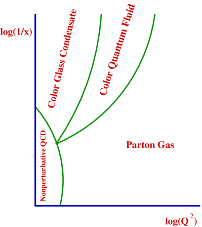
FIG. 1.: The various phases of high density QCD. (For specific numerical estimates see [17]). In the Color Glass Condensate the gluon density is large. In the Color Quantum Fluid phase, the density is low, but correlation functions are power law behaved with anomalous dimensions. In the parton gas phase, the density is described by the ordinary evolution equations of DGLAP or BFKL equation.

A problem currently not understood is the origin of the valence quark number distributions at small $x$. This includes both the baryon number distribution and isospin number distribution. Spin is also a valence effect for the distributions of quarks and gluons inside a hadron, but spin, unlike baryon number and isospin, can be carried by the gluons. We shall restrict our attention here to isospin and baryon number since it is a little simpler, although many of the techniques developed here might be applied to this case. In the case of baryon number, it is true that non-perturbative topological excitations of the gluon field might give contributions to baryon number [20, 21, 22]. For weak coupling, we expect these contributions to be small, and in this paper we shall not consider their effect. It would be most interesting to have a proper first principle computation of the magnitude of these effects within the Color Glass Condensate. An experimental analysis of the stopping of net electric charge versus the stopping of baryon number, which would allow one to disentangle the contributions of the valence quarks from the non-perturbative topological gluonic excitations at RHIC is under way [23].

We shall assume here that baryon number and isospin are carried by valence quarks [24, 25]. In weak coupling, we should be able to compute the $x$ and $Q^{2}$ dependence of these valence quark distribution functions. We will include non-perturbative aspects of the Color Glass Condensate in our computation since the quarks, although weakly coupled, propagate in the strong background field associated with the Color Glass Condensate.

In experiment, one typically measures the valence quark distribution in the distribution of particles produced in the final state. In this paper, we shall only consider how this is affected by the valence quark distribution associated with the hadron’s wavefunction. We shall not consider the effects of final state scattering. In so far as this final state scattering is due to local particle interactions, valence quantum numbers should spread diffusively, and cannot disperse over a wide range in $x$. On the other hand, novel particle interactions have been proposed, often involving the interpretation of baryon number as a topological excitation of gluons, which allow for transfer of baryon number [21, 22]. Computation of such effects is beyond the scope of this paper, but they might be possible to include in a computation such as that advocated by Krasnitz and Venugopalan [26] and by Lappi [27].

In this paper, we will derive the $x$ and $p_{T}$ dependence of the unintegrated valence quark distribution functions, subject to the caveats above. To understand the essential role that the Color Glass Condensate plays in this computation, consider the diagrams of Fig. 2 computed by Kirschner and Lipatov [28, 29, 30] and by Griffiths and Ross [31]:

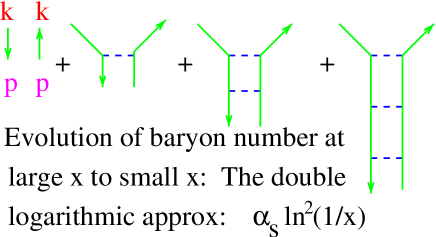
FIG. 2.: The ladder diagrams for the evolution of baryon number.

These diagrams are singular, and the expansion parameter for individual diagrams is $\alpha_{s}\ln^{2}(1/x)$. The $\ln^{2}(1/x)$ arises from the longitudinal and transverse phase space due to the fact that the $p_{T}$ integral is not limited in the ultraviolet and is effectively cut off by the center of mass energy of the system [28, 29, 30, 31].

For gluons, the expansion parameter for ladder diagrams is $\alpha_{s}\ln(1/x)$, and the result of summation is that [14]

$${{dn_{G}}\over{dx}}\sim{1\over{x^{1+C\alpha_{s}}}}.$$ (2)

For the case of valence quark distributions, we expect that the double logarithmic behavior is generated by $1/x^{\sqrt{B\alpha_{s}}}$, so it is not too surprising that the result of computing diagrams in Fig. 2 is [28]

$${{dn_{val}}\over{dx}}\sim{1\over{x^{\sqrt{2\alpha_{s}C_{F}/\pi}}}}.$$ (3)

If we take $\alpha_{s}\sim 0.25-0.5$, we find $dn_{val}/dx\sim 1/x^{0.5-0.7}$. Such a value is typical of the Color Glass Condensate and the valence quark distribution, as we shall see in a later section, correctly describes the baryon number distribution seen at RHIC.

The problem with summing the ladder graphs is justifying a weak coupling expansion [32]. If the coupling is weak, then such diagrams indeed generate the leading order contribution. On the other hand if one takes the ladder contribution seriously, the dominant contribution for baryon number occurs at a transverse momentum scale of order $\Lambda_{QCD}$, and the weak coupling methods fail. We will see that properly including the effects of the Color Glass Condensate generate a cutoff at $p_{T}\sim Q_{s}\gg\Lambda_{QCD}$ at asymptotically small $x$.

To see how this works, consider the diagrams of Fig. 3:

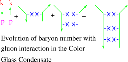
FIG. 3.: The ladder diagrams for the evolution of baryon number including the possibility of interaction with the Color Glass Condensate.

In this figure, one has a ladder sum, but the gluons can be absorbed in the Color Glass Condensate. In terms of traditional Feynman diagrams this implies that any number of gluonic ladder fan diagrams [1, 4] can connect to the reggeon (quark) ladder depicted in Fig. 3. The overall interaction would look like set of fan diagrams consisting of a single quark ladder with any number of gluonic (BFKL [14]) ladders attached to it and to each other. The fan diagrams for gluons have been summed before in [1, 4, 6]. Here we are going to write down an equation summing up the fan diagrams with a single quark ladder. For small enough $k_{T}$ of the gluons in Fig. 3, the gluons do not propagate, they get absorbed in the target and the distribution in $p_{T}$ of the quarks does not evolve. Our expectation is therefore that we get a growing distribution function for valence quarks only if the transverse momentum of the quarks exceed the saturation momentum. The coupling constant should therefore be evaluated at $Q_{s}$.

The goal of this paper is to show that this is true by constructing and solving an evolution equation for the valence quark distribution functions. The equation is constructed in Eq. (44) and its solution with a simple model for gluon evolution is given by Eq. (71).

The resulting picture which arises for the gluon and quark distribution functions is amusing: The gluons have phase space density which is dominated by glue with $k_{T}\leq Q_{s}$ and has a logarithmic divergence $\sim\ln Q_{s}/k_{T}$ in the infrared. The valence quarks have a similar transverse phase space density, which is lower than the gluon one by powers of Bjorken $x$ (see Eqs. (86), (87) and (88) and is described by the quark saturation scale $Q_{s}^{quark}=(2/3)\,Q_{s}$. This is shown in Fig. 4.

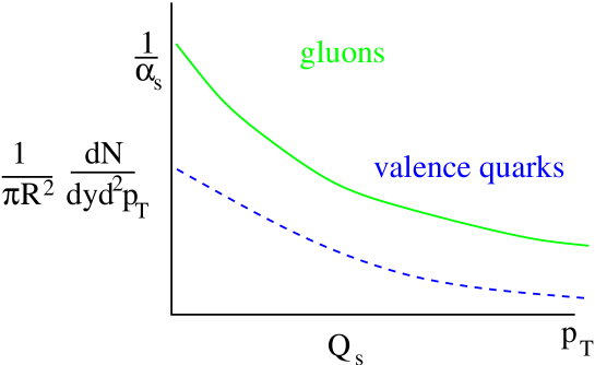
FIG. 4.: The phase space distribution of valence quarks and gluons as a function of $p_{T}$ at fixed $x$.

A remarkable conclusion of this work is that for $p_{T}$ far outside the saturation region, the valence quark distributions are power law behaved with non-integer powers (for fixed coupling). This reflects the power law behavior with fractional anomalous dimensions found for the gluon distribution function in the geometrical scaling region [10, 11]. It adds weight to the conjecture that there is an intermediate phase between that of the Color Glass Condensate and the parton gas, the Color Quantum Fluid [33].

The outline of this paper is as follows: In Sect. II we construct the analog of the McLerran-Venugopalan model for valence quarks [2]. This illustrates with a simple model how the saturation scale regulates the valence quark distribution in the infrared. Next, in Sect. III we derive a small $x$ evolution equation for the valence quark distribution within Mueller’s dipole picture. This evolution equation is then solved in the linear regime in Sect. IV and the $x$-intercept is found to agree with previous results based upon the summation of ladder diagrams [28]. Then in Sect. V we solve the full non-linear evolution equation using a simple theta function model of the dipole scattering amplitude. This section therefore merges Sect. II and and Sect. IV illustrating how the saturation scale serves as an infrared cutoff and how quantum evolution changes the canonical dimensions in the McLerran-Venugopalan model. Finally, in Sect. VI we analyze the rapidity distribution of net-protons from the BRAHMS experiment [34] and extract a phenomenological intercept. This intercept is compared with the perturbative intercept of Sect. IV and the intercept expected from Regge theory.

II Valence Quark Distribution in the Semi-Classical Approximation

In this Section we construct a soft valence quark wave function of a nucleus in the quasi-classical approximation of McLerran-Venugopalan model [2]. This quasi-classical wave function will have some qualitative features of the full answer and will also serve as the initial condition for the evolution equation which we will construct below.

Let us consider an ultrarelativistic nucleus moving in the light cone “plus” direction. Similar to [3] we begin by constructing soft valence quark distribution in a single nucleon at the lowest order in the coupling as depicted in Fig. 5. There a valence quark with momentum $p$ splits into a quark with momentum $k$ and a gluon with momentum $p-k$. Using the rules of light-cone perturbation theory [35] the wave function of the valence quark in $A_{+}=0$ light cone gauge can be written as (see Appendix A)

$$\psi^{a}_{\sigma\lambda}({\underline{k}},{\underline{p}}-{\underline{k}},z)\,=\,g\,T^{a}\,[1+z-\sigma\lambda(1-z)]\ \frac{{\underline{\epsilon}}^{\lambda}\cdot({\underline{k}}-z\,{\underline{p}})}{({\underline{k}}-z\,{\underline{p}})^{2}},$$ (4)

where $z=k_{+}/p_{+}$, $\sigma$ is the quark’s helicity which is conserved in the splitting since quarks are assumed to be massless, $\lambda$ and $a$ are gluon’s polarization and color and ${\underline{\epsilon}}^{\lambda}$ is the gluon’s polarization vector. Transforming into transverse coordinate space we end up with

$$\psi^{a}_{\sigma\lambda}({\underline{x}}_{23},{\underline{x}}_{31},z)\,=\,g\,T^{a}\,[1+z-\sigma\lambda(1-z)]\,\delta^{2}({\underline{x}}_{31}+z\,{\underline{x}}_{23})\,\frac{i}{2\pi}\,\frac{{\underline{\epsilon}}^{\lambda}\cdot{\underline{x}}_{23}}{{\underline{x}}_{23}^{2}},$$ (5)

where ${\underline{x}}_{ij}={\underline{x}}_{i}-{\underline{x}}_{j}$ with ${\underline{x}}_{1}$ and ${\underline{x}}_{2}$ the coordinates of the quark before and after the splitting and ${\underline{x}}_{3}$ the transverse coordinate of the gluon (see Fig. 5).

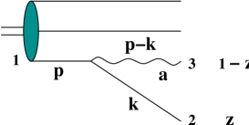
FIG. 5.: Soft valence quark wave function of a nucleon.

Squaring the expression in Eq. (5), summing over gluon polarizations, averaging over quark helicities and integrating over the initial quark position ${\underline{x}}_{1}$ (in the amplitude and in the complex conjugate amplitude separately) we end up with

$$\Psi(z)\,=\,\int\frac{d^{2}x_{23}}{2\pi}\int_{z_{i}}^{1}\frac{dz}{2(1-z)}\,\frac{1}{2}\,\sum_{\sigma,\lambda,a}|\psi^{a}_{\sigma\lambda}({\underline{x}}_{23},z)|^{2}\,=\,\int d^{2}x_{23}\,\int_{z_{i}}^{1}\,dz\,\frac{{\tilde{\alpha}}_{s}}{2\pi}\,\frac{1+z^{2}}{1-z}\,\frac{1}{x_{23}^{2}},$$ (6)

where we defined

$${\tilde{\alpha}}_{s}\,=\,\frac{\alpha_{s}C_{F}}{\pi},$$ (7)

$z_{i}$ is some initial light cone momentum fraction and $C_{F}=\frac{N_{c}^{2}-1}{2\,N_{c}}$. Looking at the $z$-dependence of Eq. (6) we recognize the real part of the DGLAP splitting function $\gamma_{qq}$ [15]. By transforming $z\rightarrow 1-z$ we would obtain $\gamma_{Gq}$ splitting function as expected.

Until now we have not imposed any restrictions on the quark’s longitudinal momentum fraction $z$. Imposing $z\ll 1$ for soft quarks we get ${\underline{x}}_{1}={\underline{x}}_{3}$ from Eq. (5). The soft valence quark wave function can be written as

$$\psi^{a}_{\sigma\lambda}({\underline{x}}_{21},z)\,=\,g\,T^{a}\,(1-\sigma\lambda)\,\frac{i}{2\pi}\,\frac{{\underline{\epsilon}}^{\lambda}\cdot{\underline{x}}_{21}}{{\underline{x}}_{21}^{2}}.$$ (8)

Let us define a distribution function of valence quarks in a nucleus similar to how it was done for gluons in [3, 36]. To do that we have to multiply the wave function in Eq. (8) by its complex conjugate at a different transverse coordinate of the soft quark, average over helicities, sum over polarizations and integrate over transverse coordinate positions of the initial quark ${\underline{x}}_{1}$. The result yields

$$\frac{dn_{val}\,({\underline{x}}-{\underline{y}})}{dy}\Bigg{|}_{LO}\,=\,\frac{1}{4\pi}\,\frac{z}{2}\,\sum_{\sigma,\lambda,a}\left<\psi^{a}_{\sigma\lambda}({\underline{x}},z)\psi^{a*}_{\sigma\lambda}({\underline{y}},z)\right>\,=\,\frac{z\,N_{c}}{2}\,A\,{\tilde{\alpha}}_{s}\,\ln\frac{1}{({\underline{x}}-{\underline{y}})^{2}\Lambda^{2}}$$ (9)

where the brackets $\left<\,\ldots\,\right>$ imply averaging over nucleon’s impact factors and summation over all nucleons in the nucleus [3, 36], which brought in a factor of atomic number $A$. We inserted a factor of $N_{c}$ in Eq. (9) to account for $N_{c}$ valence quarks in a nucleon and $\Lambda$ is some infrared cutoff of the order of $\Lambda_{QCD}$. Since we are interested in the number of quarks per unit rapidity we rewrote the $z$-integral in Eq. (6) for small $z$ as

$$\frac{dz}{1-z}\,\approx\,dz\,=\,\frac{dz}{z}\,z$$

which yielded the factor of $z$ in Eq. (9). Eq. (9) gives us the soft valence quark distribution in a nucleus at the lowest order in the coupling constant. Its Fourier transform would give us unintegrated valence quark distribution function of a nucleus.

Recalling that for soft gluons the corresponding lowest order wave function is [5]

$$A^{a}_{\sigma\lambda}({\underline{x}}_{21},z)\,=\,2\,g\,T^{a}\,\frac{i}{2\pi}\,\frac{{\underline{\epsilon}}^{\lambda}\cdot{\underline{x}}_{21}}{{\underline{x}}_{21}^{2}}$$ (10)

we obtain the LO gluon distribution function [3, 36]

$$\frac{dn_{G}\,({\underline{x}}-{\underline{y}})}{dy}\Bigg{|}_{LO}\,=\,\frac{1}{4\pi}\,\left<{\underline{A}}^{a}({\underline{x}})\cdot{\underline{A}}^{a}({\underline{y}})\right>\bigg{|}_{LO}\,=\,{\tilde{\alpha}}_{s}\,A\,\ln\frac{1}{({\underline{x}}-{\underline{y}})^{2}\Lambda^{2}}.$$ (11)

Comparing Eq. (9) to Eq. (11) we see that already at this lowest order the ratio of valence quarks to gluons in the small-$z$ tail of the distribution functions is a rapidly falling function of rapidity $y=\ln 1/z$

$$\frac{dn_{val}/dy}{dn_{G}/dy}\Bigg{|}_{LO}\,=\,\frac{z\,N_{c}}{2}\,\sim z\,\sim\,e^{-y}.$$ (12)

The exact scaling with rapidity of the ratio in Eq. (12) will be modified by quantum evolution as we will see below.

In the mean time let us try to construct the valence quark distribution function of a nucleus including the effects of multiple rescatterings [2, 3, 36]. Diagrammatically this is equivalent to resumming powers of $\alpha_{s}^{2}A^{1/3}$, or, equivalently, powers of $x_{\perp}^{2}Q_{s}^{2}$ [3]. Following the prescription carried out for gluonic fields in [3] we start off in $\partial_{\mu}A_{\mu}=0$ covariant gauge. In this gauge nucleons can not exchange gluons with each other and the soft gluonic or quark fields of the nucleus are just additive with the total field of the nucleus being the sum of the individual fields of the nucleons. Therefore if $\psi^{cov}_{N}({\underline{x}},x_{-})$ is the lowest order fermionic field of the valence quarks in a single nucleon in covariant gauge the field of the whole nucleus would be

$$\psi^{cov}_{A}({\underline{x}},x_{-})\,=\,\sum_{i=1}^{A}\psi^{cov}_{N_{i}}({\underline{x}},x_{-}).$$ (13)

After a gauge transformation to the $A_{+}=0$ light cone gauge the field becomes

$$\psi^{LC}_{A}({\underline{x}},x_{-})\,=\,S({\underline{x}},x_{-})\,\sum_{i=1}^{A}\psi^{cov}_{N_{i}}({\underline{x}},x_{-}),$$ (14)

where the matrix of gauge transformation is [3, 36]

$$S({\underline{x}},x_{-})\ =\ \mbox{P}\exp\left(-igT^{a}\int\ d^{2}b\ db_{-}\theta(x_{-}-b_{-})\ {\hat{\rho}}^{a}({\underline{b}},b_{-})\ \ln(|{\underline{x}}-{\underline{b}}|\Lambda)\right).$$ (15)

${\hat{\rho}}^{a}$ is a color charge density operator normalized according to

$$\left<{\hat{\rho}}^{a}({\underline{x}},x_{-})\ {\hat{\rho}}^{b}({\underline{y}},y_{-})\right>\ =\ \frac{\alpha_{s}}{2N_{c}\pi}\,\rho({\underline{x}},x_{-})\,\delta(x_{-}-y_{-})\,\delta^{2}({\underline{x}}-{\underline{y}})\,\delta^{ab}$$ (16)

with $\rho({\underline{x}},x_{-})$ the normal nuclear density in the infinite momentum frame of the nucleus, obeying

$$\int\ d^{2}x\ dx_{-}\ \rho({\underline{x}},x_{-})=\ A.$$ (17)

In terms of the fermionic field $\psi^{LC}_{A}({\underline{x}},x_{-})$ the valence quark distribution function can be written as

$$\frac{dn_{val}\,({\underline{x}}-{\underline{y}})}{dy}\,=\,\frac{1}{4\pi}\,\frac{z}{2}\,\int\,\frac{dx_{-}\,dy_{-}}{(2\pi)^{2}}\,e^{ik_{+}(x_{-}-\,y_{-})}\,\left<{\bar{\psi}}^{LC}_{A}({\underline{y}},y_{-})\,\frac{1}{2}\gamma_{+}\,\psi^{LC}_{A}({\underline{x}},x_{-})\right>$$ (18)

$$=\,\frac{1}{4\pi}\,\frac{z}{2}\,\int\,\frac{dx_{-}\,dy_{-}}{(2\pi)^{2}}\,e^{ik_{+}(x_{-}-\,y_{-})}\,\left<{\bar{\psi}}^{cov}_{A}({\underline{y}},y_{-})\,S^{-1}({\underline{y}},y_{-})\,\frac{1}{2}\gamma_{+}\,S({\underline{x}},x_{-})\psi^{cov}_{A}({\underline{x}},x_{-})\right>,$$ (19)

where now $\left<\ldots\right>$ includes averaging over longitudinal coordinates of the nucleons as well. The lowest order single nucleon valence quark field $\psi^{cov}_{N}({\underline{x}},x_{-})$ is the same in light cone and covariant gauges and is proportional to a $\delta$-function on the light cone, $\psi^{cov}_{N_{i}}({\underline{x}},x_{-})\sim\delta(x_{-}-x_{i-})$ with $x_{i-}$ the light cone coordinate of the nucleon. Using this property of the fermion field together with Eq. (13) in Eq. (18) yields

$$\frac{dn_{val}\,({\underline{x}}-{\underline{y}})}{dy}\,=\,\frac{1}{4\pi}\,\frac{z}{2}\,\sum_{i=1}^{A}\,\left<{\bar{\psi}}^{cov}_{N_{i}}({\underline{y}},x_{i-})\,S^{-1}({\underline{y}},x_{i-})\,\frac{1}{2}\gamma_{+}\,S({\underline{x}},x_{i-})\psi^{cov}_{N_{i}}({\underline{x}},x_{i-})\right>.$$ (20)

To perform the averaging in Eq. (20) one has to use the definition of $S({\underline{x}},x_{-})$ from Eq. (15) together with Eqs. (16) and (17) in the product $S^{-1}({\underline{y}},x_{i-})S({\underline{x}},x_{i-})$. Since the direction of $b_{-}$-integration is reversed in $S$ and $S^{-1}$ we can divide all the integration into tiny slices and the first slice on the left of $S^{-1}({\underline{y}},x_{i-})$ would include the same $b_{-}$ interval as the last slice on the right of $S({\underline{x}},x_{i-})$. Since the color charge density correlators (16) are local we can independently average in each slice keeping the correlators only up to quadratic order in $\hat{\rho}$, which corresponds to the quasi-classical approximation [3]. The same procedure has been used for different correlators in [36, 3]. Averaging of the $S$-matrices in Eq. (20) can be done independent of ${\bar{\psi}}\gamma_{+}\psi$ since the latter term is the only one depending on the slice of the $b_{-}$-integral adjacent to $x_{i-}$ (see the first reference in [3] for a discussion of the “last nucleon”). Performing $S$-matrix averaging [36] we obtain

$$\frac{dn_{val}\,({\underline{x}}-{\underline{y}})}{dy}\,=\,\frac{1}{4\pi}\,\frac{z}{2}\,\sum_{i=1}^{A}\,\int_{-L}^{L}\,\frac{dx_{i-}}{2\,L}e^{-\frac{1}{4}({\underline{x}}-{\underline{y}})^{2}\,Q_{s}^{quark\,2}\,\left(\frac{x_{i-}+L}{2\,L}\right)}\left<{\bar{\psi}}^{cov}_{N_{i}}({\underline{y}},x_{i-})\,\frac{1}{2}\gamma_{+}\,\psi^{cov}_{N_{i}}({\underline{x}},x_{i-})\right>,$$ (21)

where $2\,L$ is the extent of the nucleus in the $x_{-}$-direction. The quark saturation scale is defined for a cylindrical nucleus as [37]

$${\underline{x}}^{2}Q_{s}^{quark\,2}\,=\,{\underline{x}}^{2}\ \frac{2\pi^{2}\alpha_{s}}{N_{c}}\,\frac{A}{S_{\perp}}\,xG_{N}(x,1/{\underline{x}}^{2})$$ (22)

with $S_{\perp}=\pi R^{2}$ the cross sectional area of the nucleus with radius $R$ and $xG_{N}(x,1/{\underline{x}}^{2})={\tilde{\alpha}}_{s}\ln(1/{\underline{x}}^{2}\Lambda^{2})$ the gluon distribution in a single nucleon (see Eq. (11)).

Noting that the correlator in Eq. (21) is, in fact, $x_{i-}$-independent and is equal to the correlator in Eq. (9), we can integrate over $x_{i-}$ in Eq. (21). In the end we obtain the following expression for the valence quark structure function of a nucleus in a quasi-classical approximation

$$\frac{dn_{val}\,({\underline{x}}-{\underline{y}})}{dy}\,=\,\frac{z\,N_{c}^{2}\,S_{\perp}}{\alpha_{s}\,\pi^{2}\,({\underline{x}}-{\underline{y}})^{2}}\,\left(1-e^{-({\underline{x}}-{\underline{y}})^{2}Q_{s}^{quark\,2}/4}\right).$$ (23)

Eq. (23) has an important qualitative feature in it: the valence quark distribution goes to zero at large transverse separations $|{\underline{x}}-{\underline{y}}|$. The effect of saturation physics on the valence quark distribution function is to suppress the infrared part of the distribution. This can be observed by defining the unintegrated valence quark distribution function

$$f_{val}(x=e^{-y},{\underline{k}}^{2})\,=\,\frac{1}{4\,\pi}\,\int d^{2}x\,e^{i{\underline{k}}\cdot{\underline{x}}}\,\frac{dn_{val}\,({\underline{x}})}{dy}.$$ (24)

Neglecting the ${\underline{x}}$-dependence in $xG_{N}(x,1/{\underline{x}}^{2})$ in Eq. (22) one can Fourier-transform the expression (23) getting

$$f_{val}(x,{\underline{k}}^{2})\,=\,\frac{z\,N_{c}^{2}\,S_{\perp}}{4\,\alpha_{s}\,\pi^{2}}\ \Gamma\left(0,\frac{{\underline{k}}^{2}}{Q_{s}^{quark\,2}}\right),$$ (25)

where $\Gamma(\nu,z)$ is the incomplete Gamma function. The valence quark distribution (25) is much less infrared divergent than the Fourier transform of the lowest order expression in Eq. (9) (see Eq. (27) below). This property is similar to non-Abelian Weizsäcker-Williams gluon distribution function [3]. One can easily see that in the limit of small momenta $k_{\perp}\ll Q_{s}^{quark}$ Eq. (25) becomes

$$f_{val}(x,{\underline{k}}^{2})\,=\,\frac{z\,N_{c}^{2}\,S_{\perp}}{4\,\alpha_{s}\,\pi^{2}}\,\ln\frac{Q_{s}^{quark\,2}}{{\underline{k}}^{2}}\hskip 28.45274ptk_{\perp}\ll Q_{s}^{quark}.$$ (26)

At very high transverse momenta $k_{\perp}\gg Q_{s}^{quark}$ the valence quark distribution function (23) transformed via Eq. (24) maps onto $f_{val}(x,{\underline{k}}^{2})$ given by the lowest order expression which can be obtained by either using Eq. (9) in Eq. (24) or by expanding Eq. (25)

$$f_{val}(x,{\underline{k}}^{2})\bigg{|}_{LO}\,=\,\frac{z\,N_{c}}{2}\,A\,{\tilde{\alpha}}_{s}\,\frac{1}{{\underline{k}}^{2}},\hskip 28.45274ptk_{\perp}\gg Q_{s}^{quark}.$$ (27)

The quasi-classical approximation employed in this Section allowed us to derive two important features of the valence quark distribution at small-$x$. The first feature is that, similar to the gluon distribution, multiple rescatterings regulate the infrared singularity as demonstrated in Eqs. (23), (25) and (26). The second feature is that rapidity/Bjorken $x$ distribution of valence quarks at the classical level is just proportional to $x$ (see Eq. (12)). In the following three Sections we will study how this $x$-dependence gets modified by inclusion of quantum evolution.

III Including nonlinear evolution in the double logarithmic approximation

Our goal here is to describe the small-$x_{Bj}$ evolution of the valence quark distribution functions including the effects of gluon evolution to all orders in color charge density. We consider deep inelastic scattering (DIS) on a nucleus. In the dipole picture [5, 38] the splitting function of a virtual photon into $q\bar{q}$ dipole is factorized from the subsequent evolution of the scattering cross section of the dipole on a nucleus [4]. The total cross section and $F_{2}$ structure function are dominated by gluon exchange at small $x_{Bj}$ for which one writes

$$F_{2}(x_{Bj},Q^{2})=\frac{Q^{2}}{4\pi^{2}\alpha_{EM}}\int\frac{d^{2}x\,dz}{4\pi}\,\Phi^{\gamma^{*}\rightarrow q{\bar{q}}}({\underline{x}},z)\ 2\int d^{2}b\ N({\underline{x}},{\underline{b}},\tau\equiv\ln\frac{z_{\min}s}{\Lambda^{2}}).$$ (28)

Here $\Phi({\underline{x}},z)$ describes the photon splitting into a $\bar{q}q$ dipole with transverse separation $\underline{x}$ and moment fractions $z$ and $1-z$ respectively. To first order in the electromagnetic charge (see e.g. [39]) the photon splitting function into a $\bar{q}q$ dipole, with flavor $f$ and electromagnetic charge $(Z_{f}e)$ is

$$\Phi^{\gamma^{*}\rightarrow q\bar{q}}_{f}(\underline{x},z)=\frac{2\alpha_{EM}\ Z_{f}^{2}N_{c}}{\pi}\left[\epsilon^{2}K_{1}^{2}(\epsilon x)\left(z^{2}+(1-z)^{2}\right)+4\,Q^{2}\,z^{2}(1-z)^{2}\,K_{0}^{2}(\epsilon x)\right]\;.$$ (29)

where $\epsilon^{2}=z(1-z)Q^{2}+m_{f}^{2}$ and $m_{f}$ is the quark mass. Eq. (28) implicitly includes a sum over all quark flavors. $N({\underline{x}},{\underline{b}},\tau)$ is the forward scattering amplitude at impact parameter $\underline{b}$ of the $q\bar{q}$ dipole on a nucleus. $N(\underline{x},{\underline{b}},\tau)$ depends upon the rapidity $\tau=\ln\frac{z_{\min}s}{\Lambda^{2}}$ where $s=\frac{Q^{2}}{x_{Bj}}$ and $z_{\min}=\min(z,1-z)$. In the leading log approximation we substitute $\tau=\ln\frac{zs}{\Lambda^{2}}\approx\ln\frac{1}{x_{Bj}}$ provided that $z$ is not too small. $N({\underline{x}},{\underline{b}},\tau)$ is normalized such that

$$\sigma^{q{\bar{q}}A}_{glue}\,=\,2\int d^{2}b\,N({\underline{x}},{\underline{b}},\tau).$$ (30)

The quantum evolution of the gluon exchange amplitude $N({\underline{x}},{\underline{b}},\tau)$ has been resummed to all orders in pomeron exchanges/color charge density [4, 5, 6, 7, 8] for the total cross section of a $q\bar{q}$ dipole scattering on a nucleus. The result was a functional differential equation [7, 8]. In the large $N_{c}$ limit the small $x_{Bj}$ evolution equation for the forward amplitude $N({\underline{x}},{\underline{b}},\tau)$ is a nonlinear integro-differential equation [4, 6]

$$N({\underline{x}}_{01},{\underline{b}},\tau)=\gamma({\underline{x}}_{01},{\underline{b}})\,\exp\left[-\frac{4\alpha_{s}C_{F}}{\pi}\ln\left(\frac{x_{01}}{\rho}\right)\tau\right]+\frac{\alpha_{s}C_{F}}{\pi^{2}}\int_{0}^{\tau}d\tau^{\prime}\,\exp\left[-\frac{4\alpha_{s}C_{F}}{\pi}\ln\left(\frac{x_{01}}{\rho}\right)(\tau-\tau^{\prime})\right]$$

$$\times\int_{\rho}d^{2}x_{2}\frac{x_{01}^{2}}{x_{02}^{2}x_{12}^{2}}\,[2\,N({\underline{x}}_{02},{\underline{b}}+\frac{1}{2}{\underline{x}}_{21},\tau^{\prime})-N({\underline{x}}_{02},{\underline{b}}+\frac{1}{2}{\underline{x}}_{21},\tau^{\prime})\,N({\underline{x}}_{12},{\underline{b}}+\frac{1}{2}{\underline{x}}_{20},\tau^{\prime})],$$ (31)

where $\rho$ is some ultraviolet cutoff and $\gamma({\underline{x}}_{01},{\underline{b}})$ is the initial condition for $\tau$-evolution. In Ref. [4] $\gamma({\underline{x}}_{01},{\underline{b}})$ was taken in the quasi-classical Mueller-Glauber approximation [18]

$$\gamma({\underline{x}},{\underline{b}}_{0})=1-e^{-{\underline{x}}^{2}Q_{s}^{quark2}/4}\;.$$ (32)

The linear part of Eq. (31) gives the BFKL equation [14, 5]. Inclusion of multiple pomeron exchanges introduces the term quadratic in $N$ on the right hand side of Eq. (31). In momentum space at $t=0$ and in the double logarithmic limit Eq. (31) reduces to GLR-MQ equation [1]. We want to construct an analogue of Eq. (31) for the valence quark distribution function.

To this end, consider the difference between the structure functions of a nucleus made entirely of protons and a nucleus made entirely of neutrons, $F_{2}^{val}\equiv 3(F_{2}^{p}-F_{2}^{n})$. The gluon exchange amplitudes are identical for the proton and neutron and therefore $F_{2}^{val}$ depends upon amplitudes in which a valence quark is exchanged between the photon and the target. As before, we first factor the photon splitting function from the subsequent interaction of the $q\bar{q}$ dipole with the nucleus. Then we define the forward scattering amplitude of a dipole on a nucleus interacting with a single $\bar{q}$ exchange, $R({\underline{x}},{\underline{b}},z_{1})$, where $z_{1}$ is the light-cone momentum fraction carried by the anti-quark. As in Eq. (28), the valence quark structure function can be obtained from $R({\underline{x}},{\underline{b}},z_{1})$ by convoluting $R$ with the photon splitting function

$$F_{2}^{val}(x_{Bj},Q^{2})=\frac{Q^{2}}{4\pi^{2}\alpha_{EM}}\int\frac{d^{2}x\,dz}{4\pi}\,\Phi^{\gamma^{*}\rightarrow q{\bar{q}}}({\underline{x}},z)\ 2\int d^{2}b\ R({\underline{x}},{\underline{b}},z_{1})\;.$$ (33)

It is helpful to imagine scattering a dipole made of strange quarks (i.e. $s\bar{s}$) on a “nucleus” made up of $u\bar{d}$ dipoles in a world with three massless flavors. Then the difference between the $u\bar{u}$ and $s\bar{s}$ dipole cross sections is simply given by the reggeon exchange amplitude

$$\sigma_{val}^{q\bar{q}}\equiv\sigma_{tot}^{u\bar{u}A}-\sigma^{s\bar{s}A}_{tot}=2\int d^{2}b\ R(\underline{x},\underline{b},z_{1})\;.$$ (34)

In the quasi-classical and double logarithmic approximations considered below only the antiquark in the original dipole will be responsible for the flavor exchange interaction with the nucleus. The amplitude $R$ will therefore depend on the antiquark momentum fraction $z_{1}$ only.

To derive an evolution equation for $R(\underline{x},\underline{b},z)$ we first need to construct the quasi-classical initial conditions. The diagrams we need to sum for that are shown in Fig. 6. For gluonic evolution (31) the initial condition (32) is obtained by summing up multiple rescatterings of the dipole on the nucleons in the nucleus with two gluons exchanged with each interacting nucleon [18]. To construct initial conditions for the valence quark distribution function we modify that by replacing one of the gluonic exchanges by the quark exchange amplitude (see Fig. 6). Each quark exchange would bring in a suppression factor of $1/s$ with $s$ the center of mass energy. We therefore restrict ourselves to the leading term in this $1/s$ expansion. For simplicity, we shall make all the quarks in the nucleus and the dipole a single flavor and therefore there are $N_{c}A$ valence quarks in the nuclear wave function which can be exchanged with the dipole.

FIG. 6.: Forward amplitude of a $q\bar{q}$ pair interaction with the nucleus with one flavor-exchange interaction and all orders in gluon exchange rescatterings.

To calculate the diagram shown in Fig. 6 we start by considering only the $q{\bar{q}}$ exchange part. A simple calculation given in Appendix B yields

$$\sigma^{q\bar{q}}_{val}=\frac{2\,\alpha_{s}^{2}\,C_{F}^{2}}{N_{c}\,z_{1}\,s}\,\int\,\frac{d^{2}l}{{\underline{l}}^{2}}$$ (35)

where $s=(p+q)^{2}$ is the center of mass energy per nucleon with the virtual photon carrying momentum $q$ and the nucleon having momentum $p$. The integration over transverse momentum $l$ of the exchanged quarks in Eq. (35) is logarithmically divergent both in the infrared and in the ultraviolet. We will cut it off from below by the same infrared cutoff $\Lambda^{2}$ that we have used in the previous Section and we will cut it off from above by the maximum available relevant momentum scale in the problem — the center of mass energy $z_{1}s$ of the antiquark–nucleon system. Thus Eq. (35) becomes

$$\sigma^{q\bar{q}}_{val}=\frac{2\,\alpha_{s}^{2}\,C_{F}^{2}\,\pi}{N_{c}\,z_{1}\,s}\,\ln\frac{z_{1}\,s}{\Lambda^{2}}.$$ (36)

The effect of multiple two gluon exchanges with different nucleons is easy to calculate and gives a factor of (see e.g. [39])

$$e^{-{\underline{x}}^{2}Q_{s}^{quark\,2}/4}\;.$$ (37)

This factor is understood easily in the context of Glauber theory as $e^{-\frac{1}{2}n\sigma L}$, where $n$ is the nucleon density, $\sigma$ is dipole nucleon cross section, and $L$ is the path length of the dipole in the nucleus. The factor of $\frac{1}{2}$ arises because we are calculating the amplitude while it is the amplitude squared which gives the dipole survival probability $e^{-n\sigma L}$. The forward amplitude $R$ in the quasi-classical approximation is then

$$R_{0}({\underline{x}},{\underline{b}},z_{1})\,=\,\frac{\alpha_{s}^{2}\,C_{F}^{2}\,\pi}{z_{1}\,s}\,\frac{A}{S_{\perp}}\,\ln\frac{z_{1}\,s}{\Lambda^{2}}\,e^{-{\underline{x}}^{2}Q_{s}^{quark\,2}/4},$$ (38)

Here a factor $(N_{c}A)/S_{\perp}$ has been inserted since the antiquark can be exchange with any of the $(N_{c}A)/S_{\perp}$ quarks at a given impact parameter.

FIG. 7.: (A) Ladder diagram with the reggeized quarks in the $t$-channel and effective quark-gluon vertices considered in [29]; (B) Standard BFKL ladder diagram with reggeized gluons in the $t$-channel and effective Lipatov vertices.

Now that we have constructed the initial condition we may start building up the small-$x$ evolution. Linear equation for a BFKL-like ladder with quarks instead of gluons in the $t$-channel (see Fig. 7A) has been originally constructed in [29] and was subsequently studied in [30, 31, 40]. The resulting evolution equation has a peculiar property: due to the presence of quarks in the $t$-channel a certain part of the transverse momentum integration in the kernel is logarithmically divergent, similar to the integral in Eq. (35). The integration is effectively cut off in the ultraviolet by the center of mass energy giving an extra $\ln s$ per rung of the ladder [29]. Therefore the ladder of Fig. 7A with quarks in the $t$-channel at the leading order in $\ln s$ effectively resums powers of the parameter $\alpha_{s}\ln^{2}s$. This resummation is usually referred to as double logarithmic approximation (DLA). Note that this is in contrast to the usual BFKL ladder [14] (see Fig. 7B) which resums powers of $\alpha_{s}\ln s$ and for which DLA implies resummation of $\alpha_{s}\ln s\ln Q^{2}$. Of course the quark ladder also has an UV-safe part of the kernel resummation of which gives powers of $\alpha_{s}\ln s$ [30, 31]. However, it seems a little unclear whether resummation of higher order corrections to the DLA part of the kernel would not give contributions parametrically of the same size as iterations of the UV-safe part of the kernel. For instance NLO correction to the DLA kernel would give a parametric factor of $\alpha_{s}^{2}\ln^{2}s$, which is equivalent to double iteration of the leading logarithmic UV-safe part of the kernel $(\alpha_{s}\ln s)^{2}$. In what follows below we will work only in the double logarithmic approximation for the reggeon amplitude evolution to avoid these complications which may potentially require resummation of perturbation theory to all orders to find the leading logarithmic contribution.

At the same time we want to resum all multiple BFKL pomeron exchanges in gluon evolution similar to how it was done in [4]. Each pomeron is taken in the leading logarithmic approximation giving a parametric contribution of the order $\alpha_{s}\,\rho\,e^{C\alpha_{s}\ln s}$, where $\rho$ is proportional to the color charge density of the nucleus [2, 3] and is large ($\rho\sim\alpha_{s}\,A^{1/3}$). Therefore, even though gluon evolution will be taken below in the leading logarithmic approximation while reggeon evolution will be in the DLA limit, one can see that pomeron exchanges of the gluon evolution are enhanced by the powers of the color charge density of the source while the leading logarithmic part of reggeon evolution is not. It is therefore justified to include gluon evolution in the leading logarithmic approximation enhanced by color charge density while keeping only the DLA part of the reggeon evolution.

We want to construct an analogue of Mueller’s dipole model [5] for the reggeon amplitude $R$. To construct a dipole evolution one has to take ’t Hooft’s large $N_{c}$ limit [41] in the dipole’s wave function. The advantage of this approach is that inclusion of gluon evolution effects would become straightforward [4].

A single step of the evolution is the same as shown in Fig. 5. A hard valence quark splits into a soft quark and a hard gluon. A new color dipole $23$ is created [5]. To iterate this kernel one can write down an evolution equation which is depicted in Fig. 8. There an initial dipole $01$ either has no evolution in it at all (the first term on the right hand side in Fig. 8) or the antiquark $1$ in the dipole splits into a gluon (double line) and an antiquark $2$ creating a new dipole $12$ in addition to preexisting dipole $01$. Since we are iterating the kernel in which the antiquark $2$ is always much softer than the antiquark $1$ the transverse coordinate of the antiquark $2$ is the same on both sides of the cut. The subsequent reggeon evolution can continue in the dipole $12$ while usual gluon evolution may happen in the dipole $01$. Since in the double logarithmic approximation the virtual corrections are not important (since they do not give two logarithms of energy $s$) we can write down an equation using only the real part of the kernel (see e.g. [1, 4]).

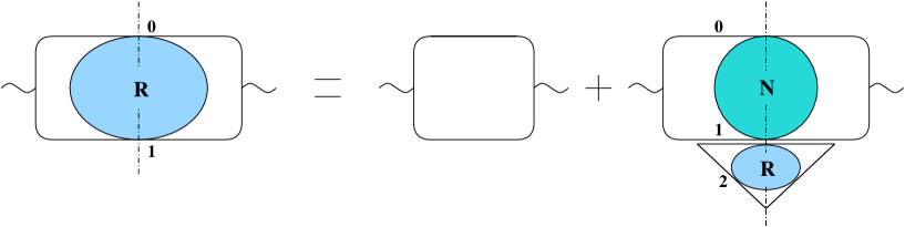
FIG. 8.: Evolution equation for the reggeon amplitude $R({\underline{x}}_{01},{\underline{b}},z_{1})$ in the double logarithmic approximation. As defined above, $R({\underline{x}}_{01},{\underline{b}},z_{1})$ is the forward amplitude of a $q\bar{q}$ dipole interacting with the nucleus by a single $\bar{q}$ exchange and many gluon exchanges, while $N({\underline{x}}_{01},{\underline{b}},z_{1})$ is the forward amplitude of a $q\bar{q}$ dipole interacting with the nucleus by gluon exchanges only.

Using the kernel of Eq. (6) with $z=z_{2}/z_{1}\ll 1$ we write

$$R({\underline{x}}_{01},{\underline{b}},z_{1})\,=\,R_{0}({\underline{x}}_{01},{\underline{b}},z_{1})\,+\,\frac{{\tilde{\alpha}}_{s}}{2\,\pi}\,\int_{z_{i}}^{z_{1}\,\mbox{min}\{1,x_{01}^{2}/x_{21}^{2}\}}\,\frac{dz_{2}}{z_{1}}\,\frac{d^{2}x_{2}}{x_{21}^{2}}\,R({\underline{x}}_{12},{\underline{b}}+\frac{1}{2}{\underline{x}}_{20},z_{2})\,$$

$$\times\,\left[1-N({\underline{x}}_{01},{\underline{b}},z_{1})\right]$$ (39)

where we have switched from rapidity notation to momentum fraction $z_{1}$ in the argument of $N$ as well. ($N$ depends on the rapidity of the softer quark or antiquark in the dipole [4, 5], which in the case of Eq. (39) is the antiquark rapidity determined by $z_{1}$. ) The first term on the right hand side of Eq. (39) corresponds to the first term on the right hand side in Fig. 8 and represents the initial conditions given by Eq. (38). The transverse coordinate integral in the second term on the right hand side of Eq. (39) is logarithmically divergent so one has to take extra care to define the limits of the $z_{2}$-integration to make it finite [29, 30, 31]. This property of the valence quark distribution’s evolution makes it very different from the usual gluonic evolution. Our goal is to order dipoles in rapidity so that each newly formed dipole would have smaller rapidity with respect to the target than the previous dipole it was produced in. In the double logarithmic approximation we can assume that the antiquark in a dipole always carries a softer light cone momentum than the quark. Defining the rapidity of dipole $01$ as $Y=\ln(z_{1}s\,x_{01}^{2})$ we would get $y=\ln(z_{2}s\,x_{12}^{2})$ for the rapidity of dipole $12$. (Dipole $01$ after splitting has roughly the same rapidity as before the splitting. Details of rapidity ordering discussed here for quarks are not important for the gluon evolution $N$.) Requiring that $Y\gg y$ we get

$$z_{2}\ll z_{1}\,\frac{x_{01}^{2}}{x_{21}^{2}},$$ (40)

which can also be obtained by requiring that the soft valence quark contribution dominates in the energy denominator. On the other hand in order to obtain logarithm of energy we need the ${\bar{q}}\rightarrow G{\bar{q}}$ splitting to produce a soft quark (see Eq. (6)). This translates into requirement that

$$z_{2}\ll z_{1}.$$ (41)

Combining Eqs. (40) and (41) we end up with

$$z_{2}\ll z_{1}\,\mbox{min}\{1,\,\frac{x_{01}^{2}}{x_{21}^{2}}\}$$ (42)

which is the upper limit used in $z_{2}$ integral in Eq. (39).

Eq. (39) together with Eq. (33) provide us with the way of determining the valence quark distribution function if the forward dipole amplitude $N$ has been found previously from Eq. (31). Defining

$$\tilde{R}({\underline{x}}_{01},{\underline{b}},z_{1})\,\equiv\,z_{1}s\,R({\underline{x}}_{01},{\underline{b}},z_{1})$$ (43)

we can rewrite Eq. (39) as

$$\tilde{R}({\underline{x}}_{01},{\underline{b}},z_{1})\,=\,\tilde{R}_{0}({\underline{x}}_{01},{\underline{b}},z_{1})\,+\,\frac{{\tilde{\alpha}}_{s}}{2\,\pi}\,\int_{z_{i}}^{z_{1}\,\mbox{min}\{1,x_{01}^{2}/x_{21}^{2}\}}\,\frac{dz_{2}}{z_{2}}\,\frac{d^{2}x_{2}}{x_{21}^{2}}\,\tilde{R}({\underline{x}}_{12},{\underline{b}}+\frac{1}{2}{\underline{x}}_{20},z_{2})\,$$

$$\times\,\left[1-N({\underline{x}}_{01},{\underline{b}},z_{1})\right].$$ (44)

Eq. (44) explicitly demonstrates that the $z_{2}$ integral of Eq. (44) is logarithmic and is similar in structure to the equation describing jet decays in the modified leading logarithmic approximation (MLLA) [42].

One can determine the scale for the running coupling constant in Eq. (44) following the prescription outlined in [43]. Since the lowest order $\alpha_{s}N_{c}$ and $\alpha_{s}N_{f}$ running coupling corrections should come together to give leading order QCD beta-function, we need to calculate only the $\alpha_{s}N_{f}$ terms to obtain the answer ($N_{f}$ if the number of flavors). Writing a dispersion relation for the gluon propagator in Fig. 5 one can show that the scale for the strong coupling constant is given by $({\underline{k}}-z{\underline{p}})^{2}/z$, such that $\alpha_{s}=\alpha_{s}[({\underline{k}}-z{\underline{p}})^{2}/z]$ [43]. In the small-$z$ limit used to obtain Eq. (44) this reduces to $\alpha_{s}({\underline{k}}^{2}/z)$. In the coordinate space for one step of the evolution (44) this translates into $\alpha_{s}[z_{1}/(z_{2}\,x_{21}^{2})]$. Therefore, running coupling effects can be included in Eq. (44) by replacing ${\tilde{\alpha}}_{s}$ in front of the integral by ${\tilde{\alpha}}_{s}[z_{1}/(z_{2}\,x_{21}^{2})]$ in the integrand. As we will see in Sect. V, the evolution equation (39) cuts off the infrared region with momenta less than $Q_{s}$ in the reggeon amplitude $R$. Similar absence of infrared diffusion was observed previously for the nonlinear evolution equation (31) in [44]. Therefore, together with the above argument, the scale of the coupling constant can, practically, only be set by either $Q_{s}$ or a higher momentum. In either case the coupling would be small for parametrically large energies. In the following, we use simply $Q_{s}$ for the running coupling scale.

IV Solution of the linear DLA equation

Let us check that the linear part of Eq. (44) is consistent with the DLA piece of the equation derived in [29] by explicitly solving it and comparing the result with [30, 31, 40]. Outside of the saturation region $N\ll 1$ [10, 11, 4] and we can neglect it on the right hand side of Eq. (44) obtaining

$$\tilde{R}({\underline{x}}_{01},z_{1})\,=\,\tilde{r}_{0}({\underline{x}}_{01},z_{1})\,+\,\frac{{\tilde{\alpha}}_{s}}{2\,\pi}\,\int_{z_{i}}^{z_{1}\,\mbox{min}\{1,x_{01}^{2}/x_{21}^{2}\}}\,\frac{dz_{2}}{z_{2}}\,\frac{d^{2}x_{2}}{x_{21}^{2}}\,\tilde{R}({\underline{x}}_{12},z_{2})$$ (45)

where $\tilde{r}_{0}({\underline{x}}_{01},z_{0},z_{1})$ is obtained from Eq. (38) by putting the exponent to be equal to $1$ so that

$$\tilde{r}_{0}({\underline{x}}_{01},z_{1})\,=\,\alpha_{s}^{2}\,C_{F}^{2}\,\pi\,\frac{A}{S_{\perp}}\,\ln\frac{z_{1}\,s}{\Lambda^{2}}\,=\,\tilde{r}^{(0)}\,\left(Y+\ln\frac{1}{x_{01}^{2}\,\Lambda^{2}}\right)$$ (46)

with

$$\tilde{r}^{(0)}\,=\,\alpha_{s}^{2}\,C_{F}^{2}\,\pi\,\frac{A}{S_{\perp}}.$$ (47)

In Eq. (45) we suppressed the impact parameter dependence neglecting the shift in ${\underline{b}}$ on the right hand side which is a good approximation for a central collision of a $q\bar{q}$ pair with a large nucleus [10, 11, 4]. Introducing Laplace transform in rapidity

$$\tilde{R}({\underline{x}}_{01},z_{1})\,=\,\int\frac{d\omega}{2\pi i}\,e^{\omega Y}\,\tilde{R}_{\omega}({\underline{x}}_{01})\,=\,\int\frac{d\omega}{2\pi i}\,(z_{1}s\,x_{01}^{2})^{\omega}\,\tilde{R}_{\omega}({\underline{x}}_{01})$$ (48)

we rewrite Eq. (45) as

$$\omega\,\tilde{R}_{\omega}(x_{01})\,=\,\left(\frac{1}{\omega}+\ln\frac{1}{x_{01}^{2}\,\Lambda^{2}}\right)\,\tilde{r}^{(0)}\,+\,\frac{{\tilde{\alpha}}_{s}}{2}\,\int_{0}^{\infty}\frac{dx_{21}^{2}}{x_{21}^{2}}\,\left(\mbox{min}\left\{\frac{x_{21}^{2}}{x_{01}^{2}},1\right\}\right)^{\omega}\,\tilde{R}_{\omega}(x_{21})$$ (49)

where we are interested only in the azimuthally symmetric solution which is dominant at high energy. Note that we implicitly assume that rapidity $Y>0$, so that $x_{01}^{2}>1/(z_{1}\,s)$ in the first term on the right hand side of Eq. (45). Then $\omega$-integration in Eq. (48) runs parallel to imaginary axis to the right of the origin. Defining Mellin transform

$$\tilde{R}_{\omega}({\underline{x}}_{01})\,=\,\int\frac{d\lambda}{2\pi i}\,(x_{01}^{2}\Lambda^{2})^{-\lambda}\,\tilde{R}_{\omega\lambda}$$ (50)

reduces Eq. (49) to

$$\omega\,\tilde{R}_{\omega\lambda}\,=\,\frac{\omega+\lambda}{\omega\lambda^{2}}\,\tilde{r}^{(0)}\,+\,\frac{{\tilde{\alpha}}_{s}}{2}\,\frac{\omega}{\lambda(\omega-\lambda)}\,\tilde{R}_{\omega\lambda}$$ (51)

which gives

$$\tilde{R}_{\omega\lambda}\,=\,\frac{\tilde{r}^{(0)}\,(\omega^{2}-\lambda^{2})}{\omega^{2}\,\lambda\,(\omega\lambda-\lambda^{2}-\frac{{\tilde{\alpha}}_{s}}{2})}.$$ (52)

Combining Eqs. (52), (50) and (48) yields

$$\tilde{R}({\underline{x}}_{01},z_{1})\,=\,\int\frac{d\omega}{2\pi i}\,\frac{d\lambda}{2\pi i}\,(z_{1}s\,x_{01}^{2})^{\omega}\,(x_{01}^{2}\Lambda^{2})^{-\lambda}\,\frac{\tilde{r}^{(0)}\,(\omega^{2}-\lambda^{2})}{\omega^{2}\,\lambda\,(\omega\lambda-\lambda^{2}-\frac{{\tilde{\alpha}}_{s}}{2})}.$$ (53)

Performing the $\omega$-integration first in Eq. (53) we notice that for positive $Re\,\lambda$ the high energy asymptotics is dominated by the rightmost pole

$$\omega\,=\,\omega^{*}(\lambda)\,\equiv\,\lambda+\frac{{\tilde{\alpha}}_{s}}{2\,\lambda}.$$ (54)

Eq. (53) becomes

$$\tilde{R}({\underline{x}}_{01},z_{1})\,=\,\int\frac{d\lambda}{2\pi i}\,(z_{1}s\,x_{01}^{2})^{\omega^{*}(\lambda)}\,(x_{01}^{2}\Lambda^{2})^{-\lambda}\,\frac{\tilde{r}^{(0)}\,(\omega^{*2}(\lambda)-\lambda^{2})}{\lambda^{2}\,\omega^{*2}(\lambda)}.$$ (55)

The integral in Eq. (55) can be done in the saddle point approximation around the saddle point $\lambda^{*}=\sqrt{{\tilde{\alpha}}_{s}/2}$ yielding

$$\tilde{R}({\underline{x}}_{01},z_{1})\,=\,\frac{3\,\tilde{r}^{(0)}}{4\,\sqrt{\pi}}\,\left(\frac{2}{{\tilde{\alpha}}_{s}}\right)^{1/4}\,(x_{01}\,\Lambda)^{-\sqrt{2\,{\tilde{\alpha}}_{s}}}\,\frac{e^{\sqrt{2\,{\tilde{\alpha}}_{s}}\,Y}}{\sqrt{2\,{\tilde{\alpha}}_{s}\,Y}}\ e^{-\frac{\sqrt{{\tilde{\alpha}}_{s}}}{Y\sqrt{2}}\,\ln^{2}(x_{01}\Lambda)}$$ (56)

where we switched to rapidity notation with $Y=\ln(z_{1}s\,x_{01}^{2})$. The integral in Eq. (55) can, in fact, be done almost exactly as will be shown in the next Section for a more general case. Using Eq. (56) in Eq. (43) together with Eq. (47) gives

$$R({\underline{x}}_{01},z_{1})\,=\,\frac{3}{4}\,{\tilde{\alpha}}_{s}^{2}\,\pi^{2}\,\sqrt{\pi}\,\frac{A}{S_{\perp}}\,\left(\frac{2}{{\tilde{\alpha}}_{s}}\right)^{1/4}\,x_{01}^{2}\,(x_{01}\,\Lambda)^{-\sqrt{2\,{\tilde{\alpha}}_{s}}}\,\frac{e^{(\sqrt{2\,{\tilde{\alpha}}_{s}}-1)\,Y}}{\sqrt{2\,{\tilde{\alpha}}_{s}\,Y}}\ e^{-\frac{\sqrt{{\tilde{\alpha}}_{s}}}{Y\sqrt{2}}\,\ln^{2}(x_{01}\Lambda)}$$ (57)

The intercept of the reggeon in Eq. (57) is equal to

$$\alpha_{R}\,=\,\sqrt{2\,{\tilde{\alpha}}_{s}}$$ (58)

in agreement with [28, 29, 30, 31, 40] so that

$$R\,\sim\,e^{(\alpha_{R}-1)Y}\,\sim\,e^{(\sqrt{2\,{\tilde{\alpha}}_{s}}-1)\,Y}.$$ (59)

To understand the transverse coordinate dependence induced by evolution let us rewrite the initial conditions of Eq. (38) in terms of rapidity. A simple calculation yields

$$R_{0}({\underline{x}},{\underline{b}},z_{1})\,=\,\alpha_{s}^{2}\,C_{F}^{2}\,\pi\,\frac{A}{S_{\perp}}\,x_{01}^{2}\,e^{-Y}\,\left(Y+\ln\frac{1}{x_{01}^{2}\Lambda^{2}}\right)\,e^{-{\underline{x}}^{2}Q_{s}^{quark\,2}/4}.$$ (60)

Comparing Eq. (60) to Eq. (57) we see that the transverse coordinate dependence of $R$ gets modified by the factor of $(x_{01}\,\Lambda)^{-\sqrt{2\,{\tilde{\alpha}}_{s}}}$ which also agrees with the results of [28, 29, 30, 31, 40]. We see that the small-$x$ evolution makes the valence quark distribution even more sensitive to the ultraviolet region by pushing the quarks toward higher transverse momenta. Overall we conclude that we have constructed a solution of the linear part of Eq. (39) shown in Eq. (57) and found it to be in agreement with the previous studies of the perturbative reggeon [28, 29, 30, 31, 40].

V Solution of the Full Nonlinear Equation with a Simple Model for $N$

Let us consider a simple model for the for the forward dipole amplitude $N({\underline{x}}_{01},{\underline{b}},\tau)$ which has correct qualitative features in agreement with the solution of Eq. (31) [4, 6] obtained in [10, 11]. Let us take

$$N({\underline{x}}_{01},{\underline{b}},\tau)\,=\,\theta({\underline{x}}_{01}^{2}Q_{s}^{2}(\tau)-1)\;.$$ (61)

The saturation scale $Q_{s}$ changes with energy as

$$Q_{s}^{2}\,=\,\Lambda^{2}\,e^{\kappa\tau}\;,$$ (62)

where

$$\tau\,=\,\ln\frac{z\,s}{\Lambda^{2}}\;,$$ (63)

and $\kappa$ is the intercept which is usually taken to be $0.2-0.3$ [10, 11, 12]. Eq. (61) gives us the dipole amplitude $N$ which is equal to one inside the saturation region and is zero otherwise. In the spirit of the theta-function approximation we also model the initial conditions of Eq. (44) given in Eq. (38) by

$${\tilde{R}}_{0}({\underline{x}}_{01},\tau)\,=\,{\tilde{r}}^{(0)}\,\tau\,\theta(1-{\underline{x}}_{01}^{2}Q_{s}^{2}(\tau)).$$ (64)

Plugging Eqs. (61) and (64) into Eq. (44) we immediately see that the solution for ${\tilde{R}}({\underline{x}}_{01},z)$ is zero inside the saturation region and can therefore be parameterized as

$${\tilde{R}}({\underline{x}}_{01},z)\,=\,\theta(1-{\underline{x}}_{01}^{2}Q_{s}^{2}(\tau))\,{\tilde{R}}_{1}({\underline{x}}_{01},z),$$ (65)

where we again suppress the impact parameter dependence. Substituting Eq. (65) together with Eqs. (61) and (64) into Eq. (44) we obtain

$${\tilde{R}}_{1}(\eta,Y)\,=\,{\tilde{r}}^{(0)}\,p\,(Y+\eta)+\frac{{\tilde{\alpha}}_{s}\,p}{2}\,\int_{0}^{Y}dY^{\prime}\,\int_{0}^{\eta+Y-Y^{\prime}}d\eta^{\prime}\,{\tilde{R}}_{1}(\eta^{\prime},Y^{\prime})$$ (66)

where we have defined

$$\eta=\ln\frac{1}{x_{\perp}^{2}Q_{s}^{2}}$$ (67)

and made use of the fact that

$$Y\,=\,\ln(z\,s\,x_{\perp}^{2})\,=\,\frac{\tau}{p}-\eta$$ (68)

with

$$p\equiv\frac{1}{1-\kappa}.$$ (69)

For simplicity we have also assumed that

$$\tau_{in}\,\equiv\,\ln\frac{z_{i}\,s}{\Lambda^{2}}\,=\,0.$$ (70)

Note that $\eta,Y>0$.

To solve Eq. (66) we reduce it to partial differential equation, determine the boundary conditions from the original integral equation, and then solve the differential equation using Laplace transform methods. This is done in Appendix C. The complete solution is

$${\tilde{R}}_{1}(\eta,Y)\,=\,\frac{\tilde{r}^{(0)}p}{\gamma}\,\left[\frac{Y+\eta}{\sqrt{Y(Y+\eta)}}\,I_{1}(2\gamma\sqrt{Y(Y+\eta)})-\frac{(Y(Y+\eta))^{3/2}}{(Y+\eta)^{3}}\,I_{3}(2\gamma\sqrt{Y(Y+\eta)})\right]$$ (71)

where we have defined $\gamma\equiv\sqrt{\frac{{\tilde{\alpha}}_{s}\,p}{2}}$.

When $Y$ is large and $\frac{\eta}{Y}$ is small, we may rewrite this formula by first employing the asymptotic expansion of the Bessel function and subsequently expanding as a function of $\frac{\eta}{Y}$

$$\tilde{R}_{1}(\eta,Y_{s})\,=\,\frac{\tilde{r}^{(0)}p}{\gamma}\,\frac{1}{\sqrt{\pi}}\frac{e^{2\gamma\,Y_{s}}}{(\gamma\,Y_{s})^{3/2}}e^{-\gamma\,\eta}\,\left[\,1+\gamma\,\eta\,\right]\;,$$ (72)

where we have defined the rapidity at the saturation boundary

$$Y_{s}\equiv\ln\,\frac{z\,s}{Q_{s}^{2}}\;.$$ (73)

Re-expressing this result in terms of $z$ and $zs\,R(\underline{x},z)=\tilde{R}(\underline{x},z)=\theta\left(1-x^{2}_{\perp}Q_{s}^{2}\right)\tilde{R}_{1}(\underline{x},z)$, we have

$$R(\underline{x},z)\,=\,\frac{\tilde{r}^{(0)}}{\gamma^{5/2}\sqrt{\pi}}\frac{1}{zs}\left(\frac{z\,s}{Q_{s}^{2}}\right)^{2\gamma}\left(x_{\perp}^{2}Q_{s}^{2}\right)^{\gamma}\left[\frac{1-\gamma\log(x_{\perp}^{2}Q_{s}^{2})}{\left(\log\frac{zs}{Q_{s}^{2}}\right)^{3/2}}\right]\,\theta\left(1-x^{2}_{\perp}Q_{s}^{2}\right)\;.$$ (74)

Next we can estimate the behavior of $F_{2}^{val}(x_{Bj},Q^{2})$ at large $Q^{2}$ and small $x_{Bj}$. To determine $F_{2}^{val}(x_{Bj},Q^{2})$ we substitute Eq. (29) for photon wave function and Eq. (74) for $R(z,\underline{r})$ into Eq. (33) for $F_{2}^{val}$. For large $Q^{2}$ the integrand falls off very rapidly due to asymptotic descent of the modified Bessel functions. Thus the integral is dominated by the region when $\epsilon^{2}r^{2}=Q^{2}r^{2}z(1-z)$ is small. This occurs when $z<\frac{1}{r^{2}Q^{2}}$ for $r$ larger than $\frac{1}{Q^{2}}$. (The region near $z=1$ is suppressed relative to $z=0$ as can be seen from Eq. (74) .) For small values of $\epsilon r$ we approximate $K_{1}(\epsilon r)\approx\frac{1}{\epsilon r}$ and neglect the corresponding contribution from $K_{0}(\epsilon r)\approx-\log(\epsilon r)$ to find

$$F_{2}^{val}(x_{Bj},Q^{2})=\frac{Q^{2}}{4\pi s}\int_{\frac{1}{Q^{2}}}^{\frac{1}{Q_{s}^{2}}}\frac{d^{2}r}{r^{2}}\int_{0}^{\frac{1}{r^{2}Q^{2}}}\frac{dz}{z}\tilde{R}_{1}(\underline{r},z)\;.$$ (75)

Next we neglect the logarithmic dependencies in the square brackets of Eq. (74) and perform the integrals over $z$ and $r$. The result for $F_{2}(x,Q^{2})$ is

$$F_{2}^{val}(x,Q^{2})\sim\left(\frac{Q^{2}}{Q_{s}^{2}}\right)^{\gamma}\,x\left(\frac{1}{x}\right)^{2\gamma}$$ (76)

Using the leading twist relation between $F_{2}^{val}$ and the valence quark phase space distribution [45]

$$F_{2}^{val}(x,Q^{2})=\int^{Q^{2}}dk^{2}\,x\frac{dn_{val}}{dx\,d^{2}k}\;,$$ (77)

we may differentiate $F_{2}^{val}$ and determine the parametric behavior of the unintegrated distribution function.

$$\frac{dn_{val}}{dx\,d^{2}k}\sim\left(\frac{Q_{s}^{2}}{k^{2}}\right)^{1-\gamma}\left(\frac{1}{x}\right)^{2\gamma}\;.$$ (78)

A number of features warrant discussion. First, quantum evolution generates an anomalous dimension of $-\gamma$ which enhances the valence quark distribution by a factor of $\sim\left(\frac{Q_{s}^{2}}{k^{2}}\right)^{-\gamma}$ relative to the naive distribution $\sim\left(\frac{Q_{s}^{2}}{k^{2}}\right)$. Second, the intercept found for the linear case in Sect. IV , $\alpha_{R}=\sqrt{2{\tilde{\alpha}}_{s}}$, differs from the intercept found here where saturation effects were fully included,

$$\alpha_{R}=\sqrt{\frac{2{\tilde{\alpha}}_{s}}{1-\kappa}}.$$ (79)

The factor $(1-\kappa)^{-\frac{1}{2}}$, reflects the fact that the saturation scale $Q_{s}^{2}=\Lambda^{2}e^{\kappa\tau}$ is serving as an infrared cutoff which increases with collision energy.

VI Relation to RHIC data on baryon stopping

The discussion presented above addressed the issue of valence quark distributions in a single nucleus. To compare obtained results with the experimental data produced in heavy ion collisions at RHIC one has to calculate valence quark production cross section. In principle the problem can be formulated in a way similar to the gluon production problem in the saturation framework [46, 36, 26, 47]. First one should solve the quasi-classical problem of including all multiple rescatterings in the valence quark production cross section [46, 36, 26, 47] and then one should continue by including the effects of quantum evolution in the obtained expression [37]. The above program has been carried out for gluon production in DIS and pA collisions in [36, 37]. However for nuclear (AA) collisions the gluon production problem complicates tremendously and still remains to be solved [26, 47]. Here we are not going to try to solve the problem of valence quark production. Rather we are going to make some $qualitative$ comparisons with the $AA$ net-proton data assuming that the produced net baryons are simply proportional to the sum of the valence quarks in the incoming nuclear wave functions.

The two nuclei collide with beam rapidities $Y_{B}$ and $-Y_{B}$. At rapidity $y$, the valence quark content (per unit rapidity) of the right moving wave function is $x_{R}f_{val}(x_{R},Q_{s}^{2})$, where $x_{R}=e^{-(Y_{B}-y)}$. Similarly the valence quark content of the left moving wavefunction is $x_{L}f_{val}(x_{L},Q_{s}^{2})$ where $x_{L}=e^{-(Y_{B}+y)}$. Thus we expect the net baryon number to scale as

$$\frac{dN^{net}_{B}}{dk^{2}dy}\sim x_{R}f_{val}(x_{R},Q_{s}^{2})+x_{L}f_{val}(x_{L},Q_{s}^{2})$$ (80)

We will parametrize, $xf_{val}(x,Q_{s}^{2})$ with a power law $\sim\left(x\right)^{\Delta_{R}}$ . This parametrization is motivated by Regge phenomenology and $\Delta_{R}$ is therefore referred to as the Reggeon intercept below. Therefore the rapidity dependence of the net baryons is given by

$$\frac{dN^{net}_{B}}{dk^{2}dy}\sim e^{-\Delta_{R}(Y_{B}-y)}+e^{-\Delta_{R}(Y_{B}+y)}\;.$$ (81)

In the small $x$ regime we expect the Reggeon intercept to be given by the formula

$$\Delta_{R}=1-2\gamma\equiv 1-2\,\sqrt{\frac{\alpha_{s}C_{F}}{2\pi}}\;.$$ (82)

We have fitted the observed net baryon distribution with the functional form given by Eq. (81) and determined the Reggeon intercept. Fig. 9 shows the fit curve with $\Delta_{R}=0.47$ together with the naive intercept $\Delta_{R}=1$. The naive intercept completely fails to reproduce the data. The remaining curve $\Delta_{R}=0.35$ will be discussed shortly.

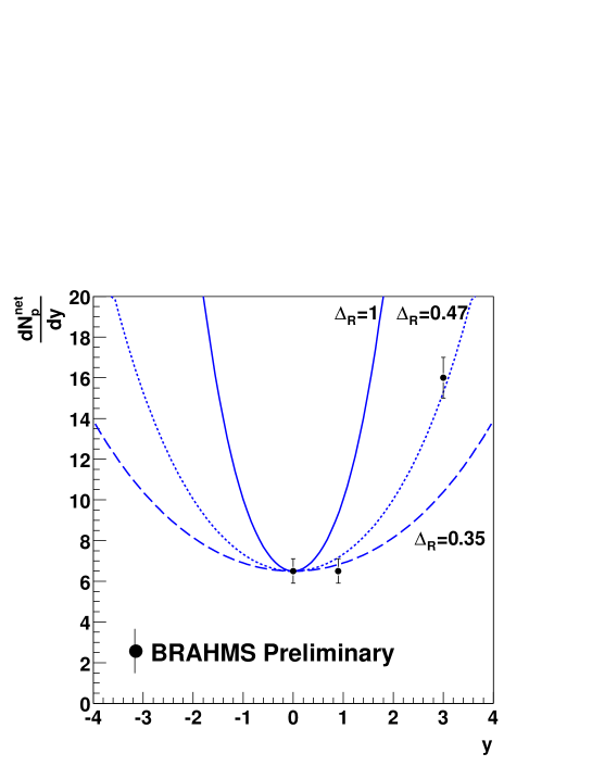
FIG. 9.: A comparison to preliminary BRAHMS data [34] on net-proton rapidity distributions with the functional form given by Eq. (81).

The value of $\Delta_{R}=0.47$ should be compared to the the non-perturbative reggeon intercept. Indeed, within the context of Regge theory valence quark transfer at high energy is given by the $I=1$ Regge trajectory, $\rho,f_{2},\omega_{3},\dots\;$. Fits to the $\pi^{-}p$ and $\pi^{+}p$ cross sections give [48]

$$\sigma_{tot}^{\pi^{-}p} = 13.63\,s^{0.0808}+36.02\,s^{-0.4525}$$ (83)

$$\sigma_{tot}^{\pi^{+}p} = 13.63\,s^{0.0808}+27.56\,s^{-0.4525}$$ (84)

The difference in these cross sections is proportional to the forward amplitude with valence quark exchange. Thus in Regge theory the exchange amplitude scales as, $R\sim s^{-0.4525}\sim x^{0.4525}$. This prediction of Regge theory that $\Delta_{R}=0.4525$ seems to agree rather well with the BRAHMS preliminary net-proton rapidity distributions.

We wish to compare the fitted intercept with Eq. (82). The current state of theory is not sufficient to compare in detail with RHIC data on net-baryon production. In addition, many of the approximations of the Color Glass Condensate are stretched in the kinematic window of the data. Nevertheless, it is useful to compare Eq. (81) to the net-baryons produced in the RHIC experiment in order to verify that this theoretical result is not in immediate contradiction with data.

Employing the phenomenological analysis of [49], we estimate the saturation scale at the rapidity $y$

$$Q_{s}^{2}(y)=Q_{s}^{2}(0)e^{-\kappa y}$$ (85)

where $Q_{s}^{2}(0)=2.05$ GeV² and $\kappa\approx 0.25$. Thus at $y=3$ we find $Q_{s}^{2}(y=3)\approx 1.0$ GeV² which is not a very large scale. Very roughly then, $\alpha_{s}(Q_{s})$ varies from $0.33-0.50$ as $y$ varies from $0-3$ units of rapidity and is not particularly small. Of course the calculations leading to Eq. (82) require $\alpha_{s}\ll 1$ or $Q_{s}^{2}/\Lambda^{2}_{QCD}\gg 1$.

Further we estimate $x$ in the kinematic window of the BRAHMS data. For the right moving nucleus we have roughly, $x_{R}=e^{-(Y_{B}-y)}$ which varies between $0.005-0.1$ in as $y$ varies between $0-3$ units of rapidity. Thus $x_{R}$ is also not particularly small as we move forward in rapidity.

Pressing onward, we substitute $\alpha_{s}=0.5$ and $\alpha_{s}=0.33$ into Eq. (82) and determine $\Delta_{R}\approx 0.35$ and $\Delta_{R}\approx 0.47$, respectively. Thus, provided the coupling is small, the perturbative Reggeon (Eq. (82)) also reproduces the experimental intercept although with many more qualifications than the non-perturbative Reggeon.

Recent data from the $dAu$ run from the RHIC collider probed the effects of gluon saturation in a nucleus [50, 51, 52, 53]. The experiments show little or no suppression of moderate to high $p_{T}$ hadrons at mid-rapidity [50, 51, 52, 53]. These data do not favor the prediction of high-$p_{T}$ hadron suppression made in [54] based on extending small-$x$ evolution to high-$p_{T}\sim Q_{s}$. Thus it would seem that the experiments have already ruled out $\log(1/x)$ evolution in this kinematic domain. However, a number of points should be considered. First, baryon number evolution is governed by double logarithms $\alpha_{s}\log^{2}(1/x)$ as opposed to single logarithms $\alpha_{s}\log(1/x)$ in the gluon case. Thus it is reasonable to hope that evolution effects are stronger in baryons than the corresponding effects in gluons. Second, multiple rescatterings [55, 56, 57, 58, 59, 60, 61, 62] which were not considered in [54] introduce the Cronin enhancement [63] in $R^{dA}$. The effect of small-$x$ evolution is to reduce this enhancement, eventually wiping out the Cronin effect at very high energies [64, 65]. However, the effect of small-$x$ evolution at moderately high energy is to somewhat reduce the Cronin maximum without eliminating it completely. Strictly speaking, the prediction of high-$p_{T}$ hadron suppression is only for $p_{T}\gg Q_{s}$ and beyond the Cronin maximum. For RHIC kinematics this means $p_{T}\gtrsim 5.0$ GeV which corresponds to rather large Bjorken $x\gtrsim 0.06$. This value of $x$ is significantly larger than the values of $x$ relevant to net-baryon production at mid-rapidity $x\approx 0.01$. Therefore, it is not obvious that $dAu$ data constrains the bulk properties of net-baryon production calculated here. Away from mid-rapidity (at say $y=3$) $x$ becomes larger $\approx 0.1$, our calculation of net-baryon production is no longer reliable, and indeed the experiments rule out strong evolution effects for these values of $x$. Between $y=0$ and $y=3$ the calculation provides a qualitative guide to the relative contributions of kinematic effects (leading to $\Delta_{R}=1$) and kinematic+quantum effects (leading to $\Delta_{R}=1-\sqrt{2C_{F}\alpha_{s}/\pi}$). For these reasons we feel that the comparison with data is instructive if not completely justified.

VII Conclusions

We have studied how isospin and baryon number are transported to small $x$. In particular we have studied how parton saturation affects the valence quark distribution. We first constructed the analog of the McLerran-Venugopalan (MV) model for valence quarks (Sect. II). The model illustrates how multiple rescatterings regulate the infrared singularities in the valence quark distribution. The saturation scale serves as an energy dependent infrared regulator as for the gluon case. For large transverse momentum, the valence quark phase space distribution at the quasi-classical level is

$$\frac{dn_{val}}{dy\,d^{2}k}\propto x\,\left(\frac{Q_{s}^{2}}{k^{2}}\right)\;,$$ (86)

where $y=\log\left(\frac{1}{x}\right)$.

Employing Mueller’s dipole framework we subsequently constructed a small $x$ evolution equation for the forward scattering amplitude with valence quark exchange between the dipole and the target (Sect. III). This equation illustrates how saturation influences the evolution of valence quark quantum numbers to small $x$. Indeed, as indicated by Eq. (39), quantum evolution stops as unitarity constraints set in.

Next we investigated the solutions of the small $x$ evolution equation in the linear and non-linear regions (Sect. IV and Sect. V). In the linear region, the solution reproduces the $x$ intercept found previously by summing ladder diagrams with quark exchange[28]. Quantum evolution enhances the valence quark rapidity distribution relative to the MV model, changing the $x$ dependence from $x$ to

$$\left(x\right)^{1-\sqrt{\frac{2\alpha_{s}C_{F}}{\pi}}}.$$ (87)

Using a simple theta function model for the dipole scattering amplitude $N(\underline{x},\underline{b},\tau)$, we then studied how parton saturation and the dynamics of the Color Glass Condensate influence the $x$ evolution of valence quarks. As in the MV model, we found that the saturation scale acts as an infrared regulator which increases with energy as $Q_{s}^{2}=\Lambda^{2}e^{\kappa\tau}$. The effect of quantum evolution is to change the canonical dimensions of the valence quark distribution. For large transverse momentum, we found

$$\frac{dn_{val}}{dy\,d^{2}k}\propto\left(\frac{Q_{s}^{2}}{k^{2}}\right)^{1-\gamma}x^{1-2\gamma},\;\;\mbox{where}\;\;\gamma\equiv\sqrt{\frac{\alpha_{s}C_{F}}{2\pi\,\left(1-\kappa\right)}}\;.$$ (88)

The intercept $\Delta_{R}=1-2\gamma$ is very similar to the intercept in the linear regime differing only by a factor of $(1-\kappa)^{-1/2}$ in $\gamma$. This difference reflects the increase of the saturation scale with energy.

Finally we studied net-baryon rapidity distributions at RHIC and extracted a phenomenological intercept from the data, $\Delta_{R}\approx 0.47$. This value is in line with the expectations of Regge theory [48]. For $\alpha_{s}\approx\frac{1}{3}$ this value is also in agreement with the intercept of Eq. (87). Whether the perturbative reggeon can quantitatively explain the net-baryon data for phenomenologically relevant $x$ remains an open question. Exciting new data on valence quarks at small $x$ is coming from the $d-Au$ run at the RHIC collider and this data will provide new constraints which will ultimately settle this question.

A The Light Cone Wave Function

In this appendix we calculate the valence quark distribution in light cone wave function of a quark moving in the “plus” direction. The lowest order graph is given by Fig. 5 . Following the rules of light cone perturbation theory this graph is given by

$$\psi^{a}_{\sigma\lambda}(\underline{k},\underline{p}-\underline{k},z)=\frac{\left\langle f|H_{I}|i\right\rangle/\sqrt{k^{+}p^{+}}}{\sum_{f}p^{-}_{f}-\sum_{i}p^{-}_{i}}=\frac{gT^{a}}{(p-k)^{-}+k^{-}-p^{-}}\frac{\bar{u}_{\sigma}(k)}{\sqrt{k^{+}}}\gamma\cdot\epsilon^{\lambda}(p-k)\frac{u_{\sigma}(p)}{\sqrt{p^{+}}}\;.$$ (A1)

Here $k^{+}=zp^{+}$, $\sigma=\pm$ is the helicity of the quark, $p^{-}=p^{0}-p^{z}=\frac{p_{T}^{2}}{p^{+}}$, and we have divided the matrix element by $\sqrt{p^{+}k^{+}}$ as is conventional in the definition of $\psi^{a}_{\sigma\lambda}$. We are working in the light cone gauge $A^{+}$=0 where $\epsilon^{\lambda}(k)=(\epsilon^{+},\epsilon^{-},\underline{\epsilon}^{\lambda})=(0,\frac{2\underline{k}\cdot\underline{\epsilon}^{\lambda}}{k^{+}},\underline{\epsilon}^{\lambda})$ and $\underline{\epsilon}^{\lambda\pm}=(\frac{1}{\sqrt{2}},\pm\frac{i}{\sqrt{2}})$. Using the formulas for the matrix elements of spinors with definite helicities given in Table II of Ref. [35]

$$\frac{\bar{u}_{\sigma}(p)}{\sqrt{p^{+}}}\gamma^{+}\frac{u_{\sigma}(q)}{\sqrt{q^{+}}} = 2$$ (A2)

$$\frac{\bar{u}_{\sigma}(p)}{\sqrt{p^{+}}}\gamma^{i}_{\perp}\frac{u_{\sigma}(q)}{\sqrt{q^{+}}} = \frac{p_{\perp}^{i}-\sigma\,i\epsilon^{ij}p_{\perp}^{j}}{p^{+}}+\frac{q_{\perp}^{i}+\sigma\,i\epsilon^{ij}q_{\perp}^{j}}{q^{+}}\;,$$ (A3)

a simple calculation reduces Eq. (A1) to the wave function given in the text

$$\psi^{a}_{\sigma\lambda}({\underline{k}},{\underline{p}}-{\underline{k}},z)\,=\,g\,T^{a}\,[1+z-\sigma\lambda(1-z)]\ \frac{{\underline{\epsilon}}^{\lambda}\cdot({\underline{k}}-z\,{\underline{p}})}{({\underline{k}}-z\,{\underline{p}})^{2}}\;.$$ (A4)

B Initial Conditions for Quantum Evolution

This appendix details the steps leading to Eq. (35) for the initial conditions of the quantum evolution.

FIG. 10.: A forward scattering amplitude with $\bar{q}$ exchange.

First calculate the squared amplitude shown in Fig. 10, summing over gluon helicities and colors, and averaging over the quark and antiquark color and helicities

$$\frac{1}{(2N_{c})^{2}}\sum\left|M\right|^{2}=\frac{C_{F}^{2}g^{4}}{N_{c}}\frac{2zs}{\underline{l}^{2}}.$$ (B1)

Here we have assumed Regge kinematics (see e.g. [66]) where $-l^{2}/s\ll 1$ and where we may replace $l^{2}$ with $-\underline{l}^{2}$. Now integrate over the loop momentum associated with the final state phase space

$$\int\frac{d^{4}l}{(2\pi)^{4}}\,2\pi\delta_{+}(k_{1}^{2})\,2\pi\delta_{+}(k_{2}^{2})\;,$$ (B2)

using the delta functions to eliminate the $l^{+}$ and $l^{-}$ integrals. Dividing by the flux factor $zp_{1}^{+}p_{2}^{-}=2\,zs$ we find the total cross section with flavor exchange

$$\sigma_{val}^{q\bar{q}}=\frac{2\,C^{2}_{F}\alpha_{s}^{2}}{N_{c}\,zs}\int\frac{d^{2}\underline{l}}{\underline{l}^{2}}\;.$$ (B3)

The upper and lower limits of integral over $\underline{l}$ are discussed in the text. To relate $\sigma^{q\bar{q}}_{val}$ to a cross section of a dipole on a nucleus at a given impact parameter $\frac{d^{2}\sigma^{q\bar{q}-A}_{val}}{d^{2}b}$ , we must multiply this cross section by the flux of valence quarks in the incoming nucleus, $(N_{c}\,A)/S_{\perp}$. Thus we find

$$2\,R(\underline{x},\underline{b},z)=\frac{d^{2}\sigma_{val}^{q\bar{q}-A}}{d^{2}b}=\frac{A}{S_{\perp}}\frac{2\,C_{F}^{2}\alpha_{s}^{2}}{zs}\int\frac{d^{2}l}{l^{2}}\;.$$ (B4)

C Solution of the model non-linear evolution equation

Our goal in this appendix is to solve the model non-linear evolution equation which replaces the scattering amplitude with a theta function. The model is described fully in Section V where an evolution equation for ${\tilde{R}}_{1}(\eta,Y)$ was obtained

$${\tilde{R}}_{1}(\eta,Y)\,=\,{\tilde{r}}^{(0)}\,p\,(Y+\eta)+\frac{{\tilde{\alpha}}_{s}\,p}{2}\,\int_{0}^{Y}dY^{\prime}\,\int_{0}^{\eta+Y-Y^{\prime}}d\eta^{\prime}\,{\tilde{R}}_{1}(\eta^{\prime},Y^{\prime})\;.$$ (C1)

Here we have defined the following variables which are described fully in the text: $\tau\,\equiv\,\ln\frac{z\,s}{\Lambda^{2}},\;Q_{s}^{2}\,\equiv\,\Lambda^{2}\,e^{\kappa\tau},\;\eta\equiv\ln\frac{1}{x_{\perp}^{2}Q_{s}^{2}},\;Y\,\equiv\,\ln(z\,s\,x_{\perp}^{2}),$ and $p\,\equiv\frac{1}{1-\kappa}\;.$ $\kappa$ is the intercept and is usually taken to be $0.2-0.3$. From these definitions we derive: $\frac{\tau}{p}=\ln\frac{zs}{Q_{s}^{2}},$ and $Y=\frac{\tau}{p}-\eta\;.$ To solve this integral equation we reduce it to a partial differential equation, deduce the boundary conditions using the original integral equation, and finally solve the differential equation employing Laplace transforms.

Differentiating Eq. (C1) with respect to $\eta$ we get

$$\frac{\partial{\tilde{R}}_{1}(\eta,Y)}{\partial\eta}\,=\,{\tilde{r}}^{(0)}\,p+\frac{{\tilde{\alpha}}_{s}\,p}{2}\,\int_{0}^{Y}dY^{\prime}\,{\tilde{R}}_{1}(\eta+Y-Y^{\prime},Y^{\prime}).$$ (C2)

Differentiating Eq. (C1) with respect to $Y$ we get

$$\frac{\partial{\tilde{R}}_{1}(\eta,Y)}{\partial Y}\,=\,{\tilde{r}}^{(0)}\,p+\frac{{\tilde{\alpha}}_{s}\,p}{2}\,\int_{0}^{\eta}d\eta^{\prime}\,{\tilde{R}}_{1}(\eta^{\prime},Y)+\frac{{\tilde{\alpha}}_{s}\,p}{2}\,\int_{0}^{Y}dY^{\prime}{\tilde{R}}_{1}(\eta+Y-Y^{\prime},Y^{\prime}).$$ (C3)

Subtracting Eq. (C2) from Eq. (C3) we end up with

$$\frac{\partial{\tilde{R}}_{1}(\eta,Y)}{\partial Y}\,=\,\frac{\partial{\tilde{R}}_{1}(\eta,Y)}{\partial\eta}+\frac{{\tilde{\alpha}}_{s}\,p}{2}\,\int_{0}^{\eta}d\eta^{\prime}{\tilde{R}}_{1}(\eta^{\prime},Y).$$ (C4)

Differentiating Eq. (C4) with respect to $\eta$ we get

$$\frac{\partial^{2}{\tilde{R}}_{1}(\eta,Y)}{\partial Y\,\partial\eta}\,=\,\frac{\partial^{2}{\tilde{R}}_{1}(\eta,Y)}{\partial\eta^{2}}+\frac{{\tilde{\alpha}}_{s}\,p}{2}{\tilde{R}}_{1}(\eta,Y).$$ (C5)

The initial conditions for Eq. (C5) are given by

$${\tilde{R}}_{1}(\eta,Y=0)\,=\,{\tilde{r}}^{(0)}\,p\,\eta,$$ (C6)

which follows from Eq. (C1),

$$\frac{\partial{\tilde{R}}_{1}(\eta,Y)}{\partial Y}\Big{|}_{Y=0}\,=\,{\tilde{r}}^{(0)}\,p\,\left(1+\frac{{\tilde{\alpha}}_{s}\,p\,\eta^{2}}{4}\right),$$ (C7)

which follows from Eq. (C3) combined with Eq. (C6), and

$$\frac{\partial{\tilde{R}}_{1}(\eta,Y)}{\partial Y}\Big{|}_{\eta=0}\,=\,\frac{\partial{\tilde{R}}_{1}(\eta,Y)}{\partial\eta}\Big{|}_{\eta=0},$$ (C8)

which follows from Eq. (C4). The solution of Eq. (C5) is uniquely specified by three boundary conditions [Eqs. (C6), (C7) and (C8)], which one can see explicitly by putting it on the lattice in $\eta,Y$ space.

Let us search for solution of Eq. (C5) in the following form

$${\tilde{R}}_{1}(\eta,Y)\,=\,\int\frac{d\lambda}{2\pi i}\,e^{\omega(\lambda)Y+\lambda\eta}\,{\tilde{R}}_{\lambda},$$ (C9)

where $\omega(\lambda)$ is some unknown function of $\lambda$ and the $\lambda$-integral runs parallel to the imaginary axis to the right of the origin. Plugging Eq. (C9) into Eq. (C5) we easily obtain

$$\omega(\lambda)\,=\,\lambda+\frac{{\tilde{\alpha}}_{s}\,p}{2\lambda}$$ (C10)

so that Eq. (C9) becomes

$${\tilde{R}}_{1}(\eta,Y)\,=\,\int\frac{d\lambda}{2\pi i}\,\exp\left[\left(\lambda+\frac{{\tilde{\alpha}}_{s}\,p}{2\lambda}\right)Y+\lambda\,\eta\right]\,{\tilde{R}}_{\lambda},$$ (C11)

where ${\tilde{R}}_{\lambda}$ should be fixed by initial conditions [Eqs. (C6), (C7) and (C8)]. They translate into three equations, which are correspondingly

$$\int\frac{d\lambda}{2\pi i}\,e^{\lambda\eta}\,{\tilde{R}}_{\lambda}\,=\,{\tilde{r}}^{(0)}\,p\,\eta,$$ (C12)

$$\int\frac{d\lambda}{2\pi i}\,e^{\lambda\eta}\,\left(\lambda+\frac{{\tilde{\alpha}}_{s}p}{2\lambda}\right)\,{\tilde{R}}_{\lambda}\,=\,{\tilde{r}}^{(0)}\,p\,\left(1+\frac{{\tilde{\alpha}}_{s}\,p\,\eta^{2}}{4}\right),$$ (C13)

and

$$\int\frac{d\lambda}{2\pi i}\,\exp\left[\left(\lambda+\frac{{\tilde{\alpha}}_{s}\,p}{2\lambda}\right)Y\right]\,\frac{1}{\lambda}\,{\tilde{R}}_{\lambda}\,=\,0.$$ (C14)

Eqs. (C12) and (C13) fix ${\tilde{R}}_{\lambda}$ to be

$${\tilde{R}}_{\lambda}\,=\,\frac{{\tilde{r}}^{(0)}\,p}{\lambda^{2}}+\sum_{n=1}^{\infty}\,a_{n}\,\lambda^{n},$$ (C15)

where $a_{n}$’s are arbitrary constants, i.e. ${\tilde{R}}_{\lambda}$ is fixed by the first two conditions up to an analytic function, which is specified only by the third condition [Eq. (C14)]. Next, substitute Eq. (C15) into Eq. (C14) and perform the contour integrals using the integral representation of the modified Bessel function

$$I_{\nu}(z)=\frac{\left(\frac{1}{2}z\right)^{\nu}}{2\pi i}\int_{-\infty}^{(0+)}\,\lambda^{-1-\nu}\exp\left(\lambda+\frac{z^{2}}{4\,\lambda}\right)\,d\,\lambda\;.$$ (C16)

where the contour starts at $-\infty$ above the real axis, circles origin, and returns to $-\infty$ below the real axis. We obtain

$$0\,=\,\frac{2{\tilde{r}}^{(0)}}{{\tilde{\alpha}}_{s}}\,I_{2}(\sqrt{2{\tilde{\alpha}}_{s}\,p\,Y^{2}})+a_{1}\sqrt{\frac{{\tilde{\alpha}}_{s}\,p}{2}}\,I_{1}(\sqrt{2{\tilde{\alpha}}_{s}\,p\,Y^{2}})+a_{2}\frac{{\tilde{\alpha}}_{s}\,p}{2}\,I_{2}(\sqrt{2{\tilde{\alpha}}_{s}\,p\,Y^{2}})+\mbox{higher order }I_{m}^{\prime}s.$$ (C17)

Since all of the Bessel functions in Eq. (C17) are linearly independent and depend upon $Y$ only, the coefficient in front of each of $I_{\nu}$ should be $0$. Enforcing this condition we end up with

$$a_{2}\,=\,-\frac{4\,{\tilde{r}}^{(0)}}{p\,{\tilde{\alpha}}_{s}^{2}},\hskip 28.45274pta_{n}\,=\,0\,\,\,\,\mbox{for}\,\,\,\,n\neq 2.$$ (C18)

We thus have

$${\tilde{R}}_{\lambda}\,=\,\frac{{\tilde{r}}^{(0)}\,p}{\lambda^{2}}-\frac{4\,{\tilde{r}}^{(0)}}{p\,{\tilde{\alpha}}_{s}^{2}}\lambda^{2},$$ (C19)

which, together with Eq. (C11) gives

$${\tilde{R}}_{1}(\eta,Y)\,=\,\int\frac{d\lambda}{2\pi i}\,\exp\left[\left(\lambda+\frac{{\tilde{\alpha}}_{s}\,p}{2\lambda}\right)Y+\lambda\,\eta\right]\,{\tilde{r}}^{(0)}\,p\,\left(\frac{1}{\lambda^{2}}-\frac{4}{p^{2}\,{\tilde{\alpha}}_{s}^{2}}\lambda^{2}\right).$$ (C20)

Integrating over $\lambda$ in Eq. (C20) yields the solution quoted in the text

$${\tilde{R}}_{1}(\eta,Y)\,=\,\frac{\tilde{r}^{(0)}p}{\gamma}\,\left[\frac{Y+\eta}{\sqrt{Y(Y+\eta)}}\,I_{1}(2\gamma\sqrt{Y(Y+\eta)})-\frac{(Y(Y+\eta))^{3/2}}{(Y+\eta)^{3}}\,I_{3}(2\gamma\sqrt{Y(Y+\eta)})\right]$$ (C21)

where we have defined $\gamma\equiv\sqrt{\frac{{\tilde{\alpha}}_{s}\,p}{2}}$.

REFERENCES

- [1] L. V. Gribov, E. M. Levin, and M. G. Ryskin, Phys. Rep. 100, 1 (1983); A.H. Mueller, J.-W. Qiu, Nucl. Phys. B268, 427 (1986).
- [2] L. McLerran and R. Venugopalan, Phys. Rev. D 49, 2233 (1994) [arXiv:hep-ph/9309289]; 49, 3352 (1994) [arXiv:hep-ph/9311205]; 50, 2225 (1994) [arXiv:hep-ph/9311205].
- [3] Yu. V. Kovchegov, Phys. Rev. D 54, 5463 (1996) [arXiv:hep-ph/9605446]; 55, 5445 (1997) [arXiv:hep-ph/9701229]; J. Jalilian-Marian, A. Kovner, L. McLerran, and H. Weigert, Phys. Rev. D 55, 5414 (1997) [arXiv:hep-ph/9606337].
- [4] Yu. V. Kovchegov, Phys. Rev. D 60, 034008 (1999) [arXiv:hep-ph/9901281]; 61, 074018 (2000) [arXiv:hep-ph/9905214].
- [5] A.H. Mueller, Nucl. Phys. B415, 373 (1994); A.H. Mueller and B. Patel, Nucl. Phys. B425, 471 (1994) [arXiv:hep-ph/9403256]; A.H. Mueller, Nucl. Phys. B437, 107 (1995) [arXiv:hep-ph/9408245]; Z. Chen, A.H. Mueller, Nucl. Phys. B451, 579 (1995).
- [6] I. I. Balitsky, Nucl. Phys. B463, 99 (1996) [arXiv:hep-ph/9509348]; Phys. Rev. D 60, 014020 (1999) [arXiv:hep-ph/9812311].
- [7] J. Jalilian-Marian, A. Kovner, A. Leonidov, and H. Weigert, Nucl. Phys. B 504, 415 (1997) [arXiv:hep-ph/9701284]; Phys. Rev. D59 014014 (1999) [arXiv:hep-ph/9706377]; Phys. Rev. D59, 034007 (1999) [arXiv:hep-ph/9807462]; Erratum. D59, 099903 (1999); J. Jalilian-Marian, A. Kovner, and H. Weigert, Phys. Rev. D 59 014015 (1999) [arXiv:hep-ph/9709432]; A. Kovner, J. G. Milhano, H. Weigert, Phys. Rev. D62, 114005 (2000) [arXiv:hep-ph/0004014]; H. Weigert, Nucl. Phys. A703, 823 (2002) [arXiv:hep-ph/0004044].
- [8] E. Iancu, A. Leonidov, and L. McLerran, Nucl. Phys. A692, 583 (2001) [arXiv:hep-ph/0011241]; Phys. Lett. B510, 133 (2001) [arXiv:hep-ph/0102009]; E. Ferreiro, E. Iancu, A. Leonidov, and L. McLerran, Nucl. Phys. A703 489 (2002) [arXiv:hep-ph/0109115].
- [9] E. Iancu and L. McLerran, Phys. Lett. B510, 145 (2001) [arXiv:hep-ph/0103032].
- [10] E. Levin and K. Tuchin, Nucl. Phys. B 573, 833 (2000) [arXiv:hep-ph/9908317]; E. Levin and K. Tuchin, Nucl. Phys. A 691, 779 (2001) [arXiv:hep-ph/0012167].
- [11] E. Iancu, K. Itakura and L. McLerran, Nucl. Phys. A 708, 327 (2002) [arXiv:hep-ph/0203137].
- [12] D. N. Triantafyllopoulos, Nucl. Phys. B 648, 293 (2003) [arXiv:hep-ph/0209121]; A. H. Mueller and D. N. Triantafyllopoulos, Nucl. Phys. B 640, 331 (2002) [arXiv:hep-ph/0205167].
- [13] E. Iancu, K. Itakura and L. McLerran, Nucl. Phys. B 724, 181 (2003). [arXiv:hep-ph/0212123].
- [14] E.A. Kuraev, L.N. Lipatov and V.S. Fadin, Sov. Phys. JETP 45, 199 (1977); Ya.Ya. Balitsky and L.N. Lipatov, Sov. J. Nucl. Phys. 28, 22 (1978).
- [15] Yu. L. Dokshitzer, JETP 73, 1216 (1977); V. N. Gribov and L. N. Lipatov, Sov. J. Nucl. Phys. 15, 78 (1972); G. Altarelli and G. Parisi, Nucl. Phys. B126, 298 (1977).
- [16] A. M. Staśto, K. Golec-Biernat and J. Kwieciński, Phys. Rev. Lett. 86, 596 (2001) [arXiv:hep-ph/0007192].
- [17] E. Levin and M. Lublinsky, Nucl. Phys. A 696, 833 (2001) [arXiv:hep-ph/0104108].
- [18] A. H. Mueller, Nucl. Phys. B335, 115 (1990); L. D. McLerran and R. Venugopalan , Phys. Rev. D 59, 094002 (1999) [hep-ph/9809427].
- [19] A. H. Mueller, Nucl. Phys. B643, 501 (2002) [arXiv:hep-ph/0206216].
- [20] G. Veneziano, Nucl. Phys. B 74, 365 (1974); G. Veneziano, Phys. Lett. B 52, 220 (1974).
- [21] B. Z. Kopeliovich and B. G. Zakharov, Z. Phys. C 43, 241 (1989).
- [22] D. Kharzeev, Phys. Lett. B 378, 238 (1996) [arXiv:nucl-th/9602027].
- [23] P. Stankus, in preparation.
- [24] K. J. Eskola and K. Kajantie, Z. Phys. C 75, 515 (1997) [arXiv:nucl-th/9610015].
- [25] S. A. Bass, B. Müller and D. K. Srivastava, Phys. Rev. Lett. 91, 052302 (2003) [arXiv:nucl-th/0212103].
- [26] A. Krasnitz, R. Venugopalan, Nucl. Phys. B557, 237 (1999) [arXiv:hep-ph/9809433]; Phys. Rev. Lett. 84, 4309 (2000) [arXiv:hep-ph/9909203]; Phys. Rev. Lett. 86, 1717 (2001) [arXiv:hep-ph/0007108]; A. Krasnitz, Y. Nara, R. Venugopalan, Phys. Rev. Lett. 87, 192302 (2001) [arXiv:hep-ph/0108092]; Nucl. Phys. A717, 268 (2003) [arXiv:hep-ph/0209269], arXiv:hep-ph/0305112 .
- [27] T. Lappi, Phys. Rev. C67, 054903 (2003) [arXiv:hep-ph/0303076].
- [28] R. Kirschner and L. N. Lipatov, Nucl. Phys. B 213, 122 (1983).
- [29] R. Kirschner, Z. Phys. C 31, 135 (1986).
- [30] R. Kirschner, Z. Phys. C 67, 459 (1995) [arXiv:hep-th/9404158]; R. Kirschner, Z. Phys. C 65, 505 (1995) [arXiv:hep-th/9407085].
- [31] S. Griffiths and D. A. Ross, Eur. Phys. J. C 12, 277 (2000) [arXiv:hep-ph/9906550].
- [32] J. Bartels, H. Lotter and M. Vogt, Phys. Lett. B 373, 215 (1996) [arXiv:hep-ph/9511399].
- [33] D. Kharzeev, private communications.
- [34] J. H. Lee for the BRAHMS Collaboration, Nucl. Phys. A715 , 482c (2003), Proceedings for Quark Matter 2002.
- [35] G. P. Lepage, S. J. Brodsky, Phys. Rev. D 22, 2157 (1980).
- [36] Yu. V. Kovchegov, A.H. Mueller, Nucl. Phys. B529, 451 (1998) [arXiv:hep-ph/9802440] .
- [37] Yu. V. Kovchegov, K. Tuchin, Phys. Rev. D 65, 074026 (2002) [arXiv:hep-ph/0111362]; Yu. V. Kovchegov, Phys. Rev. D 64, 114016 (2001) [arXiv:hep-ph/0107256].
- [38] N.N. Nikolaev, B.G. Zakharov, Z. Phys. C49, 607 (1991); Z. Phys. C53, 331 (1991); Z. Phys. C64, 651 (1994); JETP 78, 598 (1994).
- [39] Y. V. Kovchegov and L. D. McLerran, Phys. Rev. D 60, 054025 (1999) [Erratum-ibid. D 62, 019901 (2000)] [arXiv:hep-ph/9903246].
- [40] B. I. Ermolaev, S. I. Manaenkov and M. G. Ryskin, Z. Phys. C 69, 259 (1996) [arXiv:hep-ph/9502262].
- [41] G. ’t Hooft, Nucl. Phys. B 75, 461 (1974).
- [42] Yu. L. Dokshitzer, S.I. Troian, V. A. Khoze in Perturbative Quantum Chromodynamics, ed. A. H. Mueller, World Scientific, Singapore, 1989.
- [43] Y. L. Dokshitzer and D. V. Shirkov, Z. Phys. C 67, 449 (1995).
- [44] K. Golec-Biernat, L. Motyka and A. M. Stasto, Phys. Rev. D 65, 074037 (2002) [arXiv:hep-ph/0110325].
- [45] R. L. Jaffe, Nucl. Phys. B 229, 205 (1983).
- [46] A. Kovner, L. McLerran, and H. Weigert, Phys. Rev. D 52, 6231 (1995) [arXiv:hep-ph/9502289]; 52, 3809 (1995) [arXiv:hep-ph/9505320]; M. Gyulassy, L. McLerran, Phys. Rev. C 56, 2219 (1997) [arXiv:nucl-th/9704034]; Yu.V. Kovchegov, D. H. Rischke, Phys. Rev. C 56, 1084 (1997) [arXiv:hep-ph/9704201]; X. Guo, Phys. Rev, D 59, 094017 (1999) [arXiv:hep-ph/9812257].
- [47] Yu. V. Kovchegov, Nucl. Phys. A692, 557 (2001) [arXiv:hep-ph/0011252]; Nucl. Phys. A698, 619c (2002).
- [48] A. Donnachie, and P.V. Landshoff, Phys. Lett. B296, 227 (1992).
- [49] D. Kharzeev and M. Nardi, Phys. Lett. B 507, 121 (2001) [arXiv:nucl-th/0012025]; D. Kharzeev and E. Levin, Phys. Lett. B 523, 79 (2001) [arXiv:nucl-th/0108006]; D. Kharzeev, E. Levin and M. Nardi, arXiv:hep-ph/0111315.
- [50] B. B. Back [PHOBOS Collaboration], Phys. Rev. Lett. 91, 072302 (2003) [arXiv:nucl-ex/0306025].
- [51] S. S. Adler [PHENIX Collaboration], Phys. Rev. Lett. 91, 072303 (2003) [arXiv:nucl-ex/0306021].
- [52] J. Adams [STAR Collaboration], Phys. Rev. Lett. 91, 072304 (2003) [arXiv:nucl-ex/0306024].
- [53] I. Arsene [BRAHMS Collaboration], Phys. Rev. Lett. 91, 072305 (2003) [arXiv:nucl-ex/0307003].
- [54] D. Kharzeev, E. Levin and L. McLerran, Phys. Lett. B 561, 93 (2003) [arXiv:hep-ph/0210332].
- [55] B. Z. Kopeliovich, J. Nemchik, A. Schafer and A. V. Tarasov, Phys. Rev. Lett. 88, 232303 (2002) [arXiv:hep-ph/0201010].
- [56] R. Baier, A. Kovner and U. A. Wiedemann, arXiv:hep-ph/0305265.
- [57] J. Jalilian-Marian, Y. Nara and R. Venugopalan, arXiv:nucl-th/0307022.
- [58] A. Accardi and M. Gyulassy, arXiv:nucl-th/0308029.
- [59] X. N. Wang, Phys. Rev. Lett. 81 (1998) 2655; M. Gyulassy and P. Levai, Phys. Lett. B 442 (1998) 1; X. N. Wang, Phys. Rev. C 61 (2000) 064910;
- [60] E. Wang and X. N. Wang, Phys. Rev. C 64 (2001) 034901; Y. Zhang, G. Fai, G. Papp, G. G. Barnafoldi and P. Levai, Phys. Rev. C 65 (2002) 034903; I. Vitev and M. Gyulassy, Phys. Rev. Lett. 89 (2002) 252301;
- [61] I. Vitev, Phys. Lett. B 562, 36 (2003);
- [62] X. N. Wang, Phys. Lett. B 565 (2003) 116; X. N. Wang, arXiv:nucl-th/0305010; X. Zhang and G. Fai, arXiv:hep-ph/0306227. G. G. Barnafoldi, G. Papp, P. Levai and G. Fai, arXiv:nucl-th/0307062.
- [63] J. W. Cronin, H. J. Frisch, M. J. Shochet, J. P. Boymond, R. Mermod, P. A. Piroue and R. L. Sumner, Phys. Rev. D 11, 3105 (1975).
- [64] J. L. Albacete, N. Armesto, A. Kovner, C. A. Salgado and U. A. Wiedemann, arXiv:hep-ph/0307179.
- [65] D. Kharzeev, Y. V. Kovchegov and K. Tuchin, arXiv:hep-ph/0307037.
- [66] J. Forshaw and D. Ross, “Quantum Chromodynamics and the Pomeron”, Cambridge University Press (1997).