IMPACT OF RECENT NEUTRINO DATA ON R-PARITY VIOLATION

We take both the bilinear and trilinear R-parity violating couplings in supersymmetric models as a source of neutrino masses and mixings. Using the solar and atmospheric data and the Chooz constraint we determine the allowed ranges of those couplings. We also estimate the effective mass for neutrinoless double beta decay in this scenario.

1 R-parity violation and its parametrization

In supersymmetric models, lepton and baryon numbers ($L$ and $B$, respectively) are not automatically conserved, unlike in the standard model. In terms of $L$ and $B$, one defines R-parity as $R_{p}=(-1)^{3B+L+2S}$, where $S$ is the spin of a particle. Stringent phenomenological limits on R-parity violating ($R_{p}\!\!\!\!\!\!/~{}~{}$) interactions$\!{}^{{\bf?},{\bf?}}$ can be found in Ref. $\!{}^{{\bf?}}$. $B$ violation has got nothing to do with neutrino mass generation, and we assume that such interactions are absent. Neutrino Majorana mass generation requires two units of $L$ violation. For this purpose, we allow both bilinear ($\mu_{i}$) and trilinear ($\lambda,\lambda^{\prime}$) interactions in the superpotential as well as the bilinear soft terms ($B_{i}$), given by,

$$W=\mu^{J}{H}_{u}L_{J}+\frac{1}{2}\lambda^{JK\ell}L_{J}L_{K}E^{c}_{\ell}+\lambda^{{}^{\prime}Jpq}L_{J}Q_{p}D^{c}_{q}+h_{u}^{pq}{H}_{u}Q_{p}U^{c}_{q}\ ,$$ (1)

where the vector $L_{J}=(H_{d},L_{i})$ with $J:4..1$. The soft supersymmetry-breaking potential is

$$V_{soft} = \frac{\tilde{m}_{u}^{2}}{2}H_{u}^{\dagger}H_{u}+\frac{1}{2}L^{J\dagger}[\tilde{m}^{2}_{L}]_{JK}L^{K}+B^{J}H_{u}L_{J}$$ (2)

$$+A^{ups}H_{u}Q_{p}U^{c}_{s}+A^{Jps}L_{J}Q_{p}D^{c}_{s}+\frac{1}{2}A^{JKl}L_{J}L_{K}E^{c}_{l}+{\rm~{}h.c.}$$

It should be noted that field redefinitions of the $H_{d},L_{i}$ fields correspond to basis changes in $L_{J}$ space and consequently the Lagrangian parameters will be altered. Hence we use the basis-independent parameters constructed in $\!{}^{{\bf?},{\bf?}}$ and write the neutrino mass matrix in terms of such parameters $\delta^{i}_{\mu},\delta^{i}_{B},\delta^{ijk}_{\lambda},\delta^{ipq}_{\lambda^{\prime}}$, which in the basis in which the sneutrino vacuum expectation values are zero correspond to the Lagrangian parameters $\mu^{i}/|\mu|$, $B^{i}/|B|$, $\lambda_{ijk}$, $\lambda^{\prime}_{ipq}$, respectively.

This talk is mainly based on the paper $\!{}^{{\bf?}}$. For previous studies of $R_{p}\!\!\!\!\!\!/~{}~{}$ effects on neutrino masses, see also Refs. $\!{}^{{\bf?},{\bf?},{\bf?}}$.

2 Generation of neutrino masses by R-parity violation

To understand the effects of the bilinear and trilinear terms on neutrino mass matrices, let us consider them one by one. First, switch on only the bilinear $\delta^{i}_{\mu}$ terms which appear in the superpotential. Such terms generate neutrino masses at the tree level which are proportional to $\delta^{i}_{\mu}\delta^{j}_{\mu}$. This constitutes a rank 1 mass matrix which leads to only one nonzero eigenvalue. This is not enough since we know that the solar and atmospheric neutrino data require at least two nonzero eigenvalues.

Then we turn on the bilinear $\delta^{i}_{B}$ terms which appear in the scalar potential. They contribute to neutrino mass at the loop level via the Grossman-Haber diagrams $\!{}^{{\bf?}}$, in which there are gauge couplings at the neutrino vertices while there are two types of $R_{p}\!\!\!\!\!\!/~{}~{}$ interactions giving rise to the $\Delta L=2$ Majorana mass via the diagram of Fig. 1. The first type has $R_{p}\!\!\!\!\!\!/~{}~{}$ couplings located at positions III $+$ IV (slepton-Higgs mixing) with contributions proportional to $\delta_{B}\delta_{B}$. In the second type, the $R_{p}\!\!\!\!\!\!/~{}~{}$ interactions are located at positions V $+$ IV (neutrino-neutralino and slepton-Higgs mixing) with contributions proportional to $\delta_{\mu}\delta_{B}$. Now, the $\delta^{i}_{\mu}$ and $\delta^{i}_{B}$ terms together give rise to two nonzero masses, while one eigenvalue still remains zero. As far as data is concerned, this scenario works $\!{}^{{\bf?}}$.

Then we turn on the trilinear interaction for $L$ violation, namely, the $\delta^{ijk}_{\lambda}$ (or $\delta^{ipq}_{\lambda^{\prime}}$) couplings. We then have loops involving the trilinear $R_{p}\!\!\!\!\!\!/~{}~{}$ couplings $\lambda$ or $\lambda^{\prime}$ at the neutrino vertices I and II in Fig. 1 (with lepton/slepton or quark/squark as propagators). They give contributions proportional to $\delta_{\lambda}\delta_{\lambda}$ (or $\delta_{\lambda^{\prime}}\delta_{\lambda^{\prime}}$). One also has the diagram of Fig. 2, where two units of $L$ violation come from positions V (neutrino-neutralino mixing) and II ($\lambda$ or $\lambda^{\prime}$ vertex). Their contribution to the neutrino mass is proportional to $\delta_{\mu}\delta_{\lambda}$ (or $\delta_{\mu}\delta_{\lambda^{\prime}}$). Now, with bilinear and trilinear terms together, all the neutrinos become massive.

Figure 1: The usual loops ($R_{p}\!\!\!\!\!\!/~{}~{}$ at I $+$ II) and the Grossman-Haber loops ($R_{p}\!\!\!\!\!\!/~{}~{}$ at III $+$ IV or V $+$ IV) contributing to the neutrino mass.

Figure 2: Loops with a gauge and a trilinear Yukawa coupling. The $R_{p}\!\!\!\!\!\!/~{}~{}$ interactions are located at V and II.

For the sake of simplicity, we set all unknown sparticle masses equal to $M_{S}$ = 100 GeV. We then obtain a neutrino mass matrix of the form

$$[m_{\nu}]_{ij} = M_{S}\left[\delta^{i}_{\mu}\delta^{j}_{\mu}+\frac{\kappa_{1}}{\cos\beta}\left(\delta^{i}_{\mu}\delta^{j}_{B}+\delta^{j}_{\mu}\delta^{i}_{B}\right)+\frac{\kappa_{1}}{\cos^{2}\beta}\delta^{i}_{B}\delta^{j}_{B}\right]$$

$$+ \kappa_{2}\left[\sum_{k,n}m_{e_{n}}m_{e_{k}}\delta_{\lambda}^{ink}\delta_{\lambda}^{jkn}+3\sum_{k,n}m_{d_{n}}m_{d_{k}}\delta_{\lambda^{\prime}}^{ink}\delta_{\lambda^{\prime}}^{jkn}\right]$$

$$+ \kappa_{3}\left[\sum_{k}m_{e_{k}}(\delta^{i}_{\mu}\delta_{\lambda}^{jkk}+\delta^{j}_{\mu}\delta_{\lambda}^{ikk})+3\sum_{k}m_{d_{k}}(\delta^{i}_{\mu}\delta_{\lambda^{\prime}}^{jkk}+\delta^{j}_{\mu}\delta_{\lambda^{\prime}}^{ikk})\right],$$

where

$$\kappa_{1}=\frac{g^{2}}{64\pi^{2}},~{}\kappa_{2}=\frac{1}{8\pi^{2}M_{S}},~{}\kappa_{3}=\frac{g}{16\pi^{2}\sqrt{2}}.$$ (4)

We have included for completeness the contributions arising from the $\delta_{\lambda^{\prime}}$ terms which we set to zero in our numerical analysis. The simplest case to consider with a common $\delta_{\mu}^{i}\equiv\delta_{\mu},\delta_{B}^{i}\equiv\delta_{B}$ and $\delta_{\lambda}^{ink}\equiv\delta_{\lambda}$ does not work as it cannot accomodate two large mixing angles for $\theta_{12}$ and $\theta_{23}$.

In our numerical analysis we take : $\delta_{\mu}^{i}$, $\delta_{B}^{i}$, $\delta_{\lambda}^{ink}\equiv\delta_{\lambda}$, $\delta_{\lambda^{\prime}}^{ink}=0$, for $i=$ 1, 2, 3, i.e., seven independent parameters. Note that a common $\delta_{\lambda}$, in addition to $\delta^{i}_{\mu}$ and $\delta^{i}_{B}$ terms, is enough to make all the neutrinos massive, and allows us to study how the presence of the trilinear interaction alters the allowed range of the bilinear parameters. Thus, the neutrino mass matrix elements will be given by,

$$m_{11} = M_{S}\left[(\delta_{\mu}^{1})^{2}+\frac{\kappa_{1}}{\cos^{2}\beta}(\delta_{B}^{1})^{2}+2\frac{\kappa_{1}}{\cos\beta}\delta_{\mu}^{1}\delta_{B}^{1}\right]+2\kappa_{3}m_{\tau}\delta_{\mu}^{1}\delta_{\lambda}+\kappa_{2}m_{\tau}^{2}\delta_{\lambda}^{2},$$

$$m_{12} = M_{S}\left[\delta_{\mu}^{1}\delta_{\mu}^{2}+\frac{\kappa_{1}}{\cos^{2}\beta}\delta_{B}^{1}\delta_{B}^{2}+\frac{\kappa_{1}}{\cos\beta}(\delta_{\mu}^{1}\delta_{B}^{2}+\delta_{\mu}^{2}\delta_{B}^{1})\right]+\kappa_{3}m_{\tau}(\delta_{\mu}^{1}\delta_{\lambda}+\delta_{\mu}^{2}\delta_{\lambda})+\kappa_{2}m_{\tau}^{2}\delta_{\lambda}^{2},$$

$$m_{22} = M_{S}\left[(\delta_{\mu}^{2})^{2}+\frac{\kappa_{1}}{\cos^{2}\beta}(\delta_{B}^{2})^{2}+2\frac{\kappa_{1}}{\cos\beta}\delta_{\mu}^{2}\delta_{B}^{2}\right]+2\kappa_{3}m_{\tau}\delta_{\mu}^{2}\delta_{\lambda}+\kappa_{2}m_{\tau}^{2}\delta_{\lambda}^{2},$$ (5)

$$m_{13} = M_{S}\left[\delta_{\mu}^{1}\delta_{\mu}^{3}+\frac{\kappa_{1}}{\cos^{2}\beta}\delta_{B}^{1}\delta_{B}^{3}+\frac{\kappa_{1}}{\cos\beta}(\delta_{\mu}^{1}\delta_{B}^{3}+\delta_{\mu}^{3}\delta_{B}^{1})\right]+\kappa_{3}m_{\tau}\delta_{\mu}^{3}\delta_{\lambda},$$

$$m_{23} = M_{S}\left[\delta_{\mu}^{2}\delta_{\mu}^{3}+\frac{\kappa_{1}}{\cos^{2}\beta}\delta_{B}^{2}\delta_{B}^{3}+\frac{\kappa_{1}}{\cos\beta}(\delta_{\mu}^{3}\delta_{B}^{2}+\delta_{\mu}^{2}\delta_{B}^{3})\right]+\kappa_{3}m_{\tau}\delta_{\mu}^{3}\delta_{\lambda},$$

$$m_{33} = M_{S}\left[(\delta_{\mu}^{3})^{2}+\frac{\kappa_{1}}{\cos^{2}\beta}(\delta_{B}^{3})^{2}+2\frac{\kappa_{1}}{\cos\beta}\delta_{\mu}^{3}\delta_{B}^{3}\right],$$

where we have employed the hierarchy of the charged fermion masses to keep only the dominant terms, i.e. those which involve $m_{\tau}$.

3 Experimental data on neutrino masses and mixings

We write the PMNS matrix, which is the rotation matrix from neutrino flavour ($f$) to mass ($i$) eigenstates, as

$$V_{fi}=\left[\begin{array}[]{ccc}c_{12}c_{13}&c_{13}s_{12}&s_{13}\\ -c_{23}s_{12}-c_{12}s_{13}s_{23}&c_{12}c_{23}-s_{12}s_{13}s_{23}&c_{13}s_{23}\\ s_{23}s_{12}-c_{12}c_{23}s_{13}&-c_{12}s_{23}-c_{23}s_{12}s_{13}&c_{13}c_{23}\end{array}\right],$$ (6)

where $c_{ij}\equiv\cos\theta_{ij}$ and $s_{ij}\equiv\sin\theta_{ij}$. We have neglected the CP phases which are not relevant for our purpose of extracting allowed ranges of new physics from oscillation analysis. We take the solar anomaly to be a consequence of $\nu_{e}$-$\nu_{\mu}$ oscillation, and the relevant mass squared difference is $\Delta m^{2}_{12}=\Delta m^{2}_{\rm solar}$. We consider the atmospheric oscillation to be between $\nu_{\mu}$ and $\nu_{\tau}$, and the relevant mass squared difference is $\Delta m^{2}_{13}\approx\Delta m^{2}_{23}=\Delta m^{2}_{\rm atm}$. After the announcement of the SNO data, the MSW-LMA oscillation is the most favoured solution with $\Delta m^{2}_{\rm solar}=(2.5-19.0)\times 10^{-5}~{}\mathrm{eV}^{2}$ and $\sin^{2}2\theta_{12}=0.61-0.95$. The SuperK atmospheric neutrino data suggest $\Delta m^{2}_{\rm atm}=(2-5)\times 10^{-3}~{}\mathrm{eV}^{2}$ with $\sin^{2}2\theta_{23}=0.88-1.0$. The Chooz and Palo Verde long baseline reactor experiments constrain $\sin^{2}\theta_{13}~{}\raisebox{-1.72218pt}{\hbox to0.0pt{$\sim$\hss}}\raisebox{1.72218pt}{$<$}~{}0.04$. Tritium $\beta$-decay requires that the absolute mass is $m_{\nu_{e}}~{}\raisebox{-1.72218pt}{\hbox to0.0pt{$\sim$\hss}}\raisebox{1.72218pt}{$<$}~{}2.2$ eV. For the references of all the experimental data, see $\!{}^{{\bf?}}$.

4 Results and conclusions

• We have performed a general scan of parameter space made up by the seven parameters (three $\delta^{i}_{\mu}$, three $\delta^{i}_{B}$, one $\delta_{\lambda}$) that appear in the mass matrix. We allow the tree-level contributions to either dominate over the loop corrections, to be on the same order as these, or to be much smaller than the loop terms. The fitted values of the couplings, satisfying all the data mentioned in the previous section, are given in table I.

• In Fig. 3 we have presented the allowed region in the $|\delta_{B}|=\sqrt{\sum_{i}(\delta^{i}_{B})^{2}}$ versus $|\delta_{\mu}|=\sqrt{\sum_{i}(\delta^{i}_{\mu})^{2}}$ plane for the combined fit. We show our results for both $\delta_{\lambda}\neq 0$ and $\delta_{\lambda}=0$. It can be seen that the allowed region increases when we admit non-zero values of $\delta_{\lambda}$. This happens due to the presence of the $\delta_{\mu}\delta_{\lambda}$ terms in the mass matrix (originating from Fig. 2) which can take either sign thus accomodating a larger region of the parameter space. This figure should be compared with Fig. 5 of Ref. $\!{}^{{\bf?}}$.

• The resulting fit strongly prefers a hierarchical mass pattern in our scenario, although a distinction between the inverted and the normal hierarchy is not possible.

• The maximum value of $m_{\rm eff}$ we have predicted (see Table 1) can hopefully be tested in the next generation of neutrinoless double beta decay experiments. The range again implies that the spectrum is not degenerate $\!{}^{{\bf?}}$.

• Allowing a non-vanishing $\delta_{\lambda^{\prime}}$ will not qualitatively change the pattern of our fit.

• The analysis was done before the first announcement of the KamLAND results. The pattern of the fit will not be qualitatively altered if we include the KamLAND data.

Couplings	Min	Max
$\delta_{\lambda}$	$-2.0\times 10^{-4}$	$2.0\times 10^{-4}$
$\delta_{\mu}^{1}$	$-6.8\times 10^{-7}$	$6.8\times 10^{-7}$
$\delta_{\mu}^{2}$	$-8.4\times 10^{-7}$	$8.4\times 10^{-7}$
$\delta_{\mu}^{3}$	$-8.4\times 10^{-7}$	$8.4\times 10^{-7}$
$\delta_{B}^{1}$	$-2.7\times 10^{-5}$	$2.7\times 10^{-5}$
$\delta_{B}^{2}$	$-3.0\times 10^{-5}$	$3.0\times 10^{-5}$
$\delta_{B}^{3}$	$-3.0\times 10^{-5}$	$3.0\times 10^{-5}$
$m_{\rm eff}({\rm eV})$	$1.9\times 10^{-3}$	$6.7\times 10^{-2}$
$\sum m_{i}({\rm eV})$	$4.9\times 10^{-2}$	$0.2$

Table 1: Allowed range of the couplings satisfying MSW-LMA, SuperK and Chooz simultaneously (with $\cos\beta=1$).

References

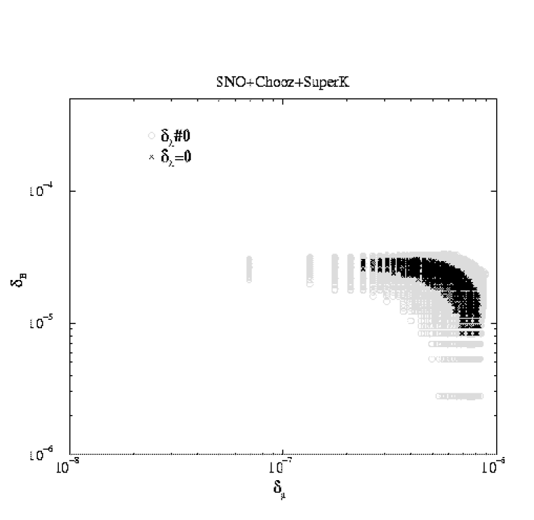
Figure 3: We present the allowed region in the $\delta_{B}\equiv|\delta_{B}|$ versus $\delta_{\mu}\equiv|\delta_{\mu}|$ plane. The circles are solutions for $\delta_{\lambda}\neq 0$, the crosses are for $\delta_{\lambda}=0$.

References

[1] H.P. Nilles and N. Polonsky,
Nucl. Phys. B 499, 33 (1997);
T. Banks, Y. Grossman, E. Nardi and Y. Nir,
Phys. Rev. D 52, 5319 (1995); F.M. Borzumati, Y. Grossman,
E. Nardi and Y. Nir, Phys. Lett. B 384, 123 (1996); E. Nardi,
Phys. Rev. D 55, 5772 (1997); L. Hall and M. Suzuki,
Nucl. Phys. B 231, 419 (1984).
[2] G. Farrar and P. Fayet, Phys. Lett. B 76, 575 (1978);
S. Weinberg, Phys. Rev. D 26, 287 (1982); N. Sakai and T. Yanagida,
Nucl. Phys. B 197, 533 (1982); C. Aulakh and R. Mohapatra,
Phys. Lett. B 119, 136 (1982).
[3] G. Bhattacharyya, hep-ph/9608415 and hep-ph/9709395;
H. Dreiner, hep-ph/9707435; B. Allanach, A. Dedes and H. Dreiner,
Phys. Rev. D 60, 075014 (1999).
[4] S. Davidson and M. Losada, JHEP0005, 021
(2000).
[5] S. Davidson and M. Losada,
Phys. Rev. D 65, 075025 (2002).
[6] A. Abada, G. Bhattacharyya and M. Losada,
Phys. Rev. D 66, 071701 (2002), Rapid Communication.
[7] A partial list is:
M. Nowakowski, A. Pilaftsis,
Nucl. Phys. B 461, 19 (1996); A.Y. Smirnov, F. Vissani,
Nucl. Phys. B 460, 37 (1996); R. Godbole, P. Roy, X. Tata,
Nucl. Phys. B 401, 67 (1993);
S. Rakshit, G. Bhattacharyya, A. Raychaudhuri, Phys. Rev. D 59, 091701 (1999); G. Bhattacharyya, H.V. Klapdor-Kleingrothaus,
H. Päs, Phys. Lett. B 463, 77 (1999); M. Drees, S. Pakvasa,
X. Tata, T. ter Veldhuis, Phys. Rev. D 57, 5335 (1998); E.J. Chun,
S.K. Kang, C.W. Kim, U.W. Lee, Nucl. Phys. B 544, 89 (1999).
[8] A. Abada and M. Losada, Nucl. Phys. B 585, 45 (2000).
[9] A. Abada and M. Losada, Phys. Lett. B 492, 310 (2000).
[10] Y. Grossman and H. Haber, Phys. Rev. Lett.78, 3438 (1997).
[11] A. Abada, S. Davidson and M. Losada,
Phys. Rev. D 65, 075010 (2002).
[12] A. Abada and G. Bhattacharyya, hep-ph/0304159.