Tau Polarization in Tau-Neutrino Nucleon Scattering

We investigate the spin polarization of $\tau^{\pm}$ leptons produced in $\nu_{\tau}$ and $\bar{\nu}_{\tau}$ nucleon scattering via charged currents. Quasi-elastic scattering, $\Delta$ resonance production and deep inelastic scattering processes are studied. The polarization information is essential for measuring the $\tau^{\pm}$ appearance rate in long baseline neutrino oscillation experiments, because the decay particle distributions depend crucially on the $\tau^{\pm}$ spin. In this article, we calculate the spin density matrix of each process and estimate the spin polarization vector in medium and high neutrino energy interactions. We find that the produced $\tau^{\pm}$’s have high degree of polarization, and their spin direction depends non-trivially on the energy and the scattering angle of $\tau^{\pm}$ in the laboratory frame.

1 Introduction

Recent studies from neutrino oscillation experiments are revealing the amazing nature of the neutrino sector, with their non-zero masses and large flavor mixings. Especially, reports from Super-Kamiokande (SK) collaboration[1] strongly suggest that nearly maximal oscillation from $\nu_{\mu}$ into $\nu_{\tau}$ is occurring in the atmospheric neutrino flux. To demonstrate this oscillation, it is important to detect $\nu_{\tau}$ appearance in oscillation experiments. Several long-baseline neutrino oscillation experiments, such as ICARUS[2], MINOS[3], OPERA[4] are proposed, and they are expected to detect the $\tau$ appearance by charged current (CC) reactions off a nucleon target

$$\nu_{\tau}(\bar{\nu}_{\tau})+N\to\tau^{-}(\tau^{+})+X$$ (1)

with $N=p,n$. Because $\tau$ production by a nucleon target has a threshold for neutrino energy at $E_{\nu}\approx 3.5$GeV, these experiments should provide high energy neutrino flux. It has also been pointed out by Hall and Murayama[5], that SK may be able to detect the $\tau$ appearance events with more than several years of running.

The produced $\tau$ decays into several particles, always including a neutrino ($\nu_{\tau}$). Therefore the $\tau$ appearance signal should be obtained from decay particle distributions. Because the $\tau$ decay distributions depend significantly on it’s spin polarization[6], the polarization information is essential for us to identify the $\tau$ production signal.

$\tau$ polarization should also be studied in order to estimate background events for the $\nu_{\mu}\to\nu_{e}$ appearance reaction, which will be searched for in neutrino oscillation experiments, such as those using high intensity neutrino beams from J-PARC[7]. Because the oscillation amplitude of $\nu_{\mu}\to\nu_{\tau}$ is larger than that of $\nu_{\mu}\to\nu_{e}$[8], and because the branching ratio of $\tau^{\mp}\to e^{\mp}+X$ is relatively large, the $e$ production via the $\nu_{\mu}\to\nu_{\tau}\to\tau\to e$ chain can be significant[9]. Since the $e$ energy and angular distribution depends crucially on the $\tau$ polarization, it’s information is necessary to estimate the background.

So far, several authors have calculated the $\tau$ production cross section for nucleon targets[5, 10, 11], but to our knowledge, no estimation of the polarization of produced $\tau$’s is available. In this paper, we study the spin polarization of $\tau$ produced by $\nu_{\tau}$ scattering off a nucleon target. We consider the quasi-elastic scattering (QE), $\Delta$ resonance production (RES), and deep inelastic scattering (DIS) processes, which are known to give dominant contributions in the medium and high neutrino energy region[10]. The spin polarization vector is obtained from the spin density matrix which is calculated for each process.

The article is organized as follows. We give the general kinematics of $\tau$ production in neutrino-nucleon interaction and the relation between the spin density matrix and the spin polarization vector in section 2. Then we present the details of the spin density matrix calculation of QE, RES, and DIS processes, in sections 3, 4, and 5, respectively. In section 6, the differential cross section and the spin polarization vector of produced $\tau^{\pm}$ are estimated for medium and high neutrino energies. Section 7 gives discussions and our conclusions.

2 Kinematics and Formalism

In this section, we show the physical regions of kinematical variables and give the relation of the $\tau$ spin polarization vector and the spin density matrix of the charged current (CC) $\tau$ production process. Firstly, we define the four-momenta of incoming neutrino ($k$), target nucleon ($p$) and produced $\tau$ lepton ($k^{\prime}$) in the laboratory frame

$$k^{\mu}\,\!\!\! = \!\!(E_{\nu},0,0,E_{\nu}),$$ (2)

$$p^{\mu}\,\!\!\! = \!\!(M,0,0,0),$$ (3)

$$k^{\prime\mu}\!\!\! = \!\!(E_{\tau},p_{\tau}\sin\theta,0,p_{\tau}\cos\theta).$$ (4)

Here, $E_{\nu}$ and $E_{\tau}$ are the incoming neutrino and outgoing $\tau$ energies, respectively, in the laboratory frame, $M$ is the nucleon mass, and $p_{\tau}=\sqrt{E_{\tau}^{2}-m_{\tau}^{2}}$ with the $\tau$ lepton mass $m_{\tau}=1.78$GeV. We also define some Lorentz invariant variables

$$Q^{2}=-q^{2},\hskip 12.0ptq^{\mu}=k^{\mu}-k^{\prime\mu},$$ (5)

$$W^{2}=(p+q)^{2}.$$ (6)

$Q^{2}$ is the magnitude of the momentum transfer and $W$ is the hadronic invariant mass. The physical regions of these variables are given by

$$M\leq W\leq\sqrt{s}-m_{\tau},$$ (7)

and

$$Q^{2}_{-}(W)\leq Q^{2}\leq Q^{2}_{+}(W),$$ (8)

where $s=(k+p)^{2}$ and

$$Q^{2}_{\pm}(W)=\frac{s-M^{2}}{2}(1\pm\bar{\beta})-\frac{1}{2}\left[W^{2}+m^{2}_{\tau}-\frac{M^{2}}{s}\left(W^{2}-m^{2}_{\tau}\right)\right]$$ (9)

with $\bar{\beta}=\lambda^{\frac{1}{2}}\left(1,m^{2}_{\tau}/s,W^{2}/s\right)$ and $\lambda(a,b,c)=a^{2}+b^{2}+c^{2}-2(ab+bc+ca)$.

The scaling variables are defined as usual:

$$x=\frac{Q^{2}}{2\,p\!\cdot\!q}=\frac{Q^{2}}{W^{2}+Q^{2}-M^{2}},$$ (10)

$$y=\frac{p\!\cdot\!q}{p\!\cdot\!k}=\frac{W^{2}+Q^{2}-M^{2}}{s-M^{2}}=1-\frac{E_{\tau}}{E_{\nu}}.$$ (11)

Here, $x$ is the Bjorken variable and $y$ is the inelasticy. The physical regions for $x$ and $y$ are obtained by Albright and Jarlskog[11, 12]:

$$\frac{m_{\tau}^{2}}{2M(E_{\nu}-m_{\tau})}\leq x\leq 1$$ (12)

and

$$A-B\leq y\leq A+B,$$ (13)

where

$$A=\frac{1}{2}\left(1-\frac{m_{\tau}^{2}}{2ME_{\nu}x}-\frac{m_{\tau}^{2}}{2E_{\nu}^{2}}\right)\bigg{/}\left(1+\frac{xM}{2E_{\nu}}\right),$$ (14)

$$B=\frac{1}{2}\left[\left(1-\frac{m_{\tau}^{2}}{2ME_{\nu}x}\right)^{2}-\frac{m_{\tau}^{2}}{E_{\nu}^{2}}\,\right]^{\frac{1}{2}}\Bigg{/}\left(1+\frac{xM}{2E_{\nu}}\right).$$ (15)

The above regions agree with those determined by Eq.(7) and Eq.(8).

We label the relevant subprocesses by using the hadronic invariant mass $W$ and the momentum transfer $Q^{2}$. We label QE (quasi-elastic scattering) when $W=M$, RES (resonance production) when $M+m_{\pi}<W<W_{\rm cut}$, and IS (inelastic scattering) when $W_{\rm cut}<W<\sqrt{s}-m_{\tau}$. $W_{\rm cut}$ is an artificial boundary between RES and IS processes, to avoid double counting. The $W_{\rm cut}$ value is taken in the region 1.4GeV$\sim$1.6GeV. Within the IS region, the region where $Q^{2}\geq 1{\rm GeV}^{2}$ may be labeled as DIS, where the use of the parton model can be justified.

Fig.1 shows the kinematical regions of each QE, RES and IS process on the $x$-$y$ plane (left) and the $p_{\tau}\cos\theta$-$p_{\tau}\sin\theta$ plane (right) at $E_{\nu}=10$ GeV. The QE region is shown by open circles, the RES region by open triangles, and the DIS region is shown by the cross symbols. The region shown by the star symbol ($\ast$) gives the IS process at low $Q^{2}$ ($Q^{2}<1{\rm GeV}^{2}$). In this region the parton model is not reliable and we must use the experimental data to reduce errors. In this report, however, we use the parton model throughout the IS region. Studies on uncertainties in this region will be reported elsewhere.

Figure 1: Physical region at $E_{\nu}=10$ GeV in the $x$-$y$ plane (left), and in the $p_{\tau}\cos\theta$-$p_{\tau}\sin\theta$ plane (right). Open circles denote QE (quasi-elastic scattering), open triangles denote RES ($\Delta$ resonance production), and the cross symbols give the DIS (deep inelastic scattering) region with $Q^{2}\geq 1\rm GeV^{2}$. The region marked by the star symbol ($\ast$) gives inelastic scattering (IS), at $W\geq 1.4$GeV and $Q^{2}<1{\rm GeV}^{2}$.

Produced $\tau$ will be partially polarized. We define the spin polarization vector, parameterized as

$$\vec{s}=(s_{x},s_{y},s_{z})=\frac{P}{2}\left(\sin\theta_{P}\cos\varphi_{P},\sin\theta_{P}\sin\varphi_{P},\cos\theta_{P}\right)$$ (16)

in the $\tau$ rest frame in which the z-axis is taken along it’s momentum direction in the laboratory frame. In Eq.(16), $\theta_{P}$ and $\varphi_{P}$ are the polar and azimuthal angle of the spin vector in the $\tau$ rest frame, respectively, and $P$ denotes the degree of polarization. $P=1$ gives the fully polarized $\tau$, and $P=0$ gives unpolarized $\tau$. The azimuthal angle is measured from the scattering plane where $\varphi_{P}={\pi}/{2}$ is along the $\vec{p}_{\nu}\times\vec{p}_{\tau}$ direction in the laboratory frame. The degree of polarization ($P$) and the spin directions ($\theta_{P},\varphi_{P}$) are functions of $E_{\tau}$ and $\cos\theta$. This spin polarization vector is related with the spin density matrix $R_{\lambda\lambda^{\prime}}$, by the following relation:

$$\frac{dR_{\lambda\lambda^{\prime}}}{dE_{\tau}\,d\cos\theta}=\frac{1}{2}\left(\begin{array}[]{cc}1+{P}\cos\theta_{P}&{P}\sin\theta_{P}\,e^{i\varphi_{P}}\\ {P}\sin\theta_{P}\,e^{-i\varphi_{P}}&1-{P}\cos\theta_{P}\end{array}\right)\!\cdot\!\frac{d\sigma_{\rm sum}}{dE_{\tau}\,d\cos\theta}.$$ (19)

The density matrix is calculated as $R_{\lambda\lambda^{\prime}}\propto\sum M_{\lambda}M^{*}_{\lambda^{\prime}}$, where $M_{\lambda}$ is the helicity amplitude with the $\tau$ helicity $\lambda/2$ defined in the laboratory frame, and $d\sigma_{\rm sum}=dR_{++}+dR_{--}$ is the usual spin summed cross section. The summation symbol implies the summation over final states, and the spins of the target and final-state particles.

The spin density matrix of $\tau$ production is obtained by using the leptonic and hadronic tensor as

$$\frac{dR_{\lambda\lambda^{\prime}}}{dE_{\tau}\,d\cos\theta}=\frac{G_{F}^{2}\kappa^{2}}{4\pi}\frac{p_{\tau}}{ME_{\nu}}\,L^{\mu\nu}_{\lambda\lambda^{\prime}}W_{\mu\nu},$$ (20)

where $G_{F}$ is Fermi constant and $\kappa=M_{W}^{2}/(Q^{2}+M_{W}^{2})$ is the propagator factor with the $W$-boson mass $M_{W}=80.4$GeV. For $\tau^{-}$ production, the leptonic tensor $L^{\mu\nu}_{\lambda\lambda^{\prime}}$ is expressed as

$$L_{\lambda\lambda^{\prime}}^{\mu\nu}=j_{\lambda}^{\mu}\,j^{*\nu}_{\lambda^{\prime}},$$ (21)

where the leptonic weak current $j_{\lambda}^{\mu}$ is

$$j_{\lambda}^{\mu}\!\!\! = \!\!\!\bar{u}_{\tau}(k^{\prime},\lambda)\,\gamma^{\mu}\frac{1-\gamma_{5}}{2}\,u_{\nu}(k)$$ (24)

$$= \!\!\!\left\{\begin{array}[]{ll}\sqrt{2E_{\nu}(E_{\tau}-p_{\tau})}\,\left(\sin\!\frac{\theta}{2},-\cos\!\frac{\theta}{2},i\cos\!\frac{\theta}{2},\sin\!\frac{\theta}{2}\right)&\ \ (\lambda=+)\\ \sqrt{2E_{\nu}(E_{\tau}+p_{\tau})}\,\left(\cos\!\frac{\theta}{2},\sin\!\frac{\theta}{2},-i\sin\!\frac{\theta}{2},\cos\!\frac{\theta}{2}\right)&\ \ (\lambda=-)\end{array}\right.$$

in the laboratory frame. For $\tau^{+}$ production, we must replace the leptonic tensor $L^{\mu\nu}_{\lambda\lambda^{\prime}}$ into $\overline{L}^{\mu\nu}_{\lambda\lambda^{\prime}}$ defined as

$$\overline{L}^{\mu\nu}_{\lambda\lambda^{\prime}}=\bar{j}^{\mu}_{\lambda}\,\bar{j}^{*\,\nu}_{\lambda^{\prime}},$$ (25)

where $\bar{j}_{\lambda}^{\mu}$ is

$$\bar{j}_{\lambda}^{\mu}\!\!\! = \!\!\!\bar{v}_{\nu}(k)\,\gamma^{\mu}\frac{1-\gamma_{5}}{2}\,v_{\tau}(k^{\prime},\lambda)$$ (28)

$$= \!\!\!\left\{\begin{array}[]{ll}\sqrt{2E_{\nu}(E_{\tau}+p_{\tau})}\,\left(\cos\!\frac{\theta}{2},\sin\!\frac{\theta}{2},i\sin\!\frac{\theta}{2},\cos\!\frac{\theta}{2}\right)&\ \ (\lambda=+)\\ \sqrt{2E_{\nu}(E_{\tau}-p_{\tau})}\,\left(-\sin\!\frac{\theta}{2},\cos\!\frac{\theta}{2},i\cos\!\frac{\theta}{2},-\sin\!\frac{\theta}{2}\right)&\ \ (\lambda=-),\\ \end{array}\right.$$

which is related with $j_{\lambda}^{\mu}$ by $\bar{j}_{\lambda}^{\mu}=\lambda\,j_{-\lambda}^{*\mu}$, in the phase convention of Ref.[13]. In the following sections, we will abbreviate the overline of the leptonic tensor and currents for $\tau^{+}$ production process.

The hadronic tensor is expressed in general as

$$W_{\mu\nu}(p,q)=-g_{\mu\nu}W_{1}(p\!\cdot\!q,Q^{2})+\frac{p_{\mu}p_{\nu}}{M^{2}}\,W_{2}(p\!\cdot\!q,Q^{2})-i\epsilon_{\mu\nu\alpha\beta}\frac{p^{\alpha}q^{\beta}}{2M^{2}}\,W_{3}(p\!\cdot\!q,Q^{2})$$

$$+\frac{q_{\mu}q_{\nu}}{M^{2}}\,W_{4}(p\!\cdot\!q,Q^{2})+\frac{p_{\mu}q_{\nu}+q_{\mu}p_{\nu}}{2M^{2}}\,W_{5}(p\!\cdot\!q,Q^{2}),$$ (29)

where the totally anti-symmetric tensor $\epsilon_{\mu\nu\alpha\beta}$ is defined as $\epsilon_{0123}=1$, and the structure functions $W_{i=1,\ldots,5}(p\cdot q,Q^{2})$ can be estimated for each subprocess. Since $q\cdot j_{\lambda}$ is proportional to $m_{\tau}$, the structure functions $W_{4}$ and $W_{5}$ appear only in the heavy lepton production case[12].

Inserting these equations into Eq.(20) and Eq.(19), we find

$$\frac{d\sigma_{\rm sum}}{dE_{\tau}\,d\cos\theta}\!\!\! = \!\!\!\frac{G_{F}^{2}\kappa^{2}}{2\pi}\frac{p_{\tau}}{M}\,\bigg{\{}\Big{(}2W_{1}+\frac{m_{\tau}^{2}}{M^{2}}\,W_{4}\Big{)}\left(E_{\tau}-p_{\tau}\cos\theta\right)+W_{2}\left(E_{\tau}+p_{\tau}\cos\theta\right)$$ (30)

$$\hskip 50.0pt\pm\frac{W_{3}}{M}\,\Big{(}E_{\nu}E_{\tau}+p_{\tau}^{2}-(E_{\nu}+E_{\tau})p_{\tau}\cos\theta\Big{)}-\frac{m_{\tau}^{2}}{M}\,W_{5}\bigg{\}}$$

$$\equiv \!\!\!\frac{G_{F}^{2}\kappa^{2}}{2\pi}\frac{p_{\tau}}{M}\;F,$$

and the spin polarization vector takes

$$s_{x}\!\!\! = \!\!\!\mp\,\frac{m_{\tau}\sin\theta}{2}\bigg{(}2W_{1}-W_{2}\pm\frac{E_{\nu}}{M}\,W_{3}-\frac{m_{\tau}^{2}}{M^{2}}\,W_{4}+\frac{E_{\tau}}{M}\,W_{5}\bigg{)}\bigg{/}F,$$ (31a)

$$s_{y}\!\!\! = \!\!\!0,$$ (31b)

$$s_{z}\!\!\! = \!\!\!\mp\,\frac{1}{2}\bigg{\{}\Big{(}2W_{1}-\frac{m_{\tau}^{2}}{M^{2}}\,W_{4}\Big{)}\left(p_{\tau}-E_{\tau}\cos\theta\right)+W_{2}\left(p_{\tau}+E_{\tau}\cos\theta\right)$$ (31c)

$$\hskip 30.0pt\pm\frac{W_{3}}{M}\,\Big{(}(E_{\nu}+E_{\tau})p_{\tau}-(E_{\nu}E_{\tau}+p_{\tau}^{2})\cos\theta\Big{)}-\frac{m_{\tau}^{2}}{M}\,W_{5}\cos\theta\bigg{\}}\bigg{/}F,$$

for $\tau^{\mp}$ productions. The degree of polarization is given by

$$P=2\sqrt{s_{x}^{2}+s_{y}^{2}+s_{z}^{2}}.$$ (32)

The above results Eq.(30)-(32) agree with Ref.[12]. From the above equations we find (i) $\varphi_{P}$ takes either 0 or $\pi$ for any $\tau$ momentum, which means that the polarization vector lies always in the scattering plane, and (ii) if $m_{\tau}=0$, then $\vec{s}$ could take only $(0,0,\mp\frac{1}{2})$, which means fully left-handed $\tau^{-}$ or right-handed $\tau^{+}$.

3 Quasi-Elastic Scattering

In this section, we give the spin density matrix calculation for the QE scattering processes

$$\nu_{\tau}+n\!\!\! \to \!\!\!\tau^{-}+p,$$ (33)

$$\bar{\nu}_{\tau}+p\!\!\! \to \!\!\!\tau^{+}+n.$$ (34)

Following Llewellyn Smith[14], the hadronic tensor is written by using the weak transition current $J_{\mu}^{(\pm)}$ as follows:

$$W^{\rm QE}_{\mu\nu}=\frac{\cos^{2}\theta_{c}}{4}\sum_{\rm spins}J_{\mu}^{(\pm)}{J^{(\pm)}_{\nu}}^{*}\,\delta(W^{2}-M^{2}),$$ (35)

where $\theta_{c}$ is the Cabibbo angle. The weak transition currents $J_{\mu}^{(+)}$ and $J_{\mu}^{(-)}$ for the $\nu_{\tau}$ and $\bar{\nu}_{\tau}$ scattering, respectively, are defined as

$$J_{\mu}^{(+)}=\langle p(p^{\prime})|\hat{J}_{\mu}^{(+)}|n(p)\rangle=\bar{u}_{p}(p^{\prime})\,\Gamma_{\mu}(p^{\prime},p)\,u_{n}(p),$$ (36)

$$J_{\mu}^{(-)}=\langle n(p^{\prime})|\hat{J}_{\mu}^{(-)}|p(p)\rangle=\bar{u}_{n}(p^{\prime})\,\overline{\Gamma}_{\mu}(p^{\prime},p)\,u_{p}(p)=\langle p(p)|\hat{J}_{\mu}^{(+)}|n(p^{\prime})\rangle^{*},$$ (37)

where $\Gamma_{\mu}$ is written in terms of the six weak form factors of the nucleon, $F^{V}_{1,2,3}$, $F_{A}$, $F_{3}^{A}$ and $F_{p}$, as

$$\Gamma_{\mu}(p^{\prime},p)=\gamma_{\mu}\,F^{V}_{1}(q^{2})\!\!\! + \!\!\!\frac{i\sigma_{\mu\alpha}q^{\alpha}\xi}{2M}\,F^{V}_{2}(q^{2})+\frac{q_{\mu}}{M}\,F^{V}_{3}(q^{2})$$ (38)

$$+ \!\!\!\left[\gamma_{\mu}\,F_{A}(q^{2})+\frac{\left(p+p^{\prime}\right)_{\mu}}{M}\,F^{A}_{3}(q^{2})+\frac{q_{\mu}}{M}\,F_{p}(q^{2})\right]\gamma_{5}.$$

For the $\bar{\nu}_{\tau}$ scattering, the vertex $\overline{\Gamma}_{\mu}$ is obtained by $\overline{\Gamma}_{\mu}(p^{\prime},p)=\gamma_{0}\Gamma_{\mu}^{\dagger}(p,p^{\prime})\gamma_{0}$. We can drop two form factors, $F^{V}_{3}$ and $F^{A}_{3}$, because of time reversal invariance and isospin symmetry (or equivalently no second-class currents). Moreover, the vector form factor $F_{1}^{V}$ and $F_{2}^{V}$ are related to the electromagnetic form factors of nucleons under the conserved vector current (CVC) hypothesis:

$$F^{V}_{1}(q^{2})={\displaystyle G^{V}_{E}(q^{2})-\frac{q^{2}}{4M^{2}}G^{V}_{M}(q^{2})\over\displaystyle 1-\frac{q^{2}}{4M^{2}}},\hskip 12.0pt\xi F^{V}_{2}(q^{2})=\frac{\displaystyle G^{V}_{M}(q^{2})-G^{V}_{E}(q^{2})}{\displaystyle 1-\frac{q^{2}}{4M^{2}}},$$ (39)

where

$$G^{V}_{E}(q^{2})=\frac{1}{\displaystyle\left(1-\frac{q^{2}}{M_{V}^{2}}\right)^{2}},\hskip 12.0ptG^{V}_{M}(q^{2})=\frac{1+\xi}{\displaystyle\left(1-\frac{q^{2}}{M_{V}^{2}}\right)^{2}},$$ (40)

with a vector mass $M_{V}=0.84$ GeV and $\xi=\mu_{p}-\mu_{n}=3.706$. $\mu_{p}$ and $\mu_{n}$ are the anomalous magnetic moments of proton and neutron, respectively. For the axial vector form factor $F_{A}$, we adopt the following parametrization:

$$F_{A}(q^{2})=\frac{F_{A}(0)}{\displaystyle\left(1-\frac{q^{2}}{M_{A}^{2}}\right)^{2}}$$ (41)

with an axial-vector mass $M_{A}=1.0$ GeV and $F_{A}(0)=-1.23$[14]. For the pseudo-scalar form factor $F_{p}$, we adopt the parametrization of Ref.[14]

$$F_{p}(q^{2})=2M^{2}\frac{F_{A}(q^{2})}{m_{\pi}^{2}-q^{2}}$$ (42)

with the pion mass $m_{\pi}=0.14$ GeV. The normalization of $F_{p}(0)$ is fixed by the partially conserved axial vector current (PCAC) hypothesis. It should be stressed here that, the form factor $F_{p}(q^{2})$ has not been measured experimentally because its contribution is proportional to the lepton mass. The production cross section and the polarization of $\tau$ are sensitive to $F_{p}(q^{2})$ because of the large $\tau$ mass and the spin-flip nature of the form factor.

In Fig.2, we show the total cross sections of the QE process versus the incoming neutrino energy. We plot not only the $\tau$-neutrino interaction process, but also the $\mu$-neutrino interaction process for comparison. Solid curves are the $\nu_{\mu}$ and $\nu_{\tau}$ scattering cross sections and dashed curves are the $\bar{\nu}_{\mu}$ and $\bar{\nu}_{\tau}$ scattering cross sections. Our results agree well with those of Hall and Murayama[5].

Figure 2: The neutrino energy dependence of the total cross sections of the QE (quasi-elastic) processes, $\nu_{l}n\to{l}^{-}p$ (solid lines) and $\bar{\nu}_{l}p\to{l}^{+}n$ (dashed lines). The thick lines are for ${l}=\tau$, while the thin lines are for ${l}=\mu$.

4 Resonance Production

In this section, we present the spin density matrix calculation for the $\Delta$ production processes

$$\nu_{\tau}+n(p)\!\!\! \to \!\!\!\tau^{-}+\Delta^{+}(\Delta^{++}),$$ (43)

$$\bar{\nu}_{\tau}+p(n)\!\!\! \to \!\!\!\tau^{+}+\Delta^{0}(\Delta^{-}).$$ (44)

We neglect $N^{*}$ and the other higher resonance states, which are known to give small contributions[10, 15, 16]. For the $\Delta$ resonance production, we calculate the hadronic tensor by using the nucleon-$\Delta$ weak transition current $J_{\mu}$ as follows:

$$W^{\rm RES}_{\mu\nu}=\frac{\cos^{2}\theta_{c}}{4}\sum_{\rm spins}J_{\mu}J^{*}_{\nu}\,\frac{1}{\pi}\,\frac{W\Gamma(W)}{(W^{2}-M_{\Delta}^{2})^{2}+W^{2}\Gamma^{2}(W)}.$$ (45)

Here, $M_{\Delta}$ is the resonance mass, $M_{\Delta}=1.232$GeV, and $\Gamma(W)$ is its running width estimated by assuming the dominance of S-wave $\Delta\to N+\pi$ decay:

$$\Gamma(W)=\Gamma(M_{\Delta})\,\frac{M_{\Delta}}{W}\frac{\lambda^{\frac{1}{2}}(W^{2},M^{2},m^{2}_{\pi})}{\lambda^{\frac{1}{2}}(M_{\Delta}^{2},M^{2},m^{2}_{\pi})}$$ (46)

with $\Gamma(M_{\Delta})=0.12$ GeV and $\lambda(a,b,c)=a^{2}+b^{2}+c^{2}-2(ab+bc+ca)$.

The current $J_{\mu}$ for the process $\nu_{\tau}+n\to\tau^{-}+\Delta^{+}$ is defined by

$$J_{\mu}=\langle\Delta^{+}(p^{\prime})|\hat{J}_{\mu}|n(p)\rangle=\bar{\psi}^{\alpha}(p^{\prime})\,\Gamma_{\mu\alpha}\,u_{n}(p),$$ (47)

where $\psi^{\alpha}$ is the spin-3/2 particle wave function and the vertex $\Gamma_{\mu\alpha}$ is expressed in terms of the eight weak form factors $C^{V,A}_{i=3,4,5,6}$[14, 17, 18, 19] as

$$\Gamma_{\mu\alpha}=\left[\frac{C^{V}_{3}}{M}\left(g_{\mu\alpha}q/-\gamma_{\mu}q_{\alpha}\right)+\frac{C^{V}_{4}}{M^{2}}\left(g_{\mu\alpha}p^{\prime}\!\cdot\!q-p^{\prime}_{\mu}q_{\alpha}\right)\right.$$

$$\left.+\frac{C^{V}_{5}}{M^{2}}\left(g_{\mu\alpha}p\!\cdot\!q-p_{\mu}q_{\alpha}\right)+\frac{C^{V}_{6}}{M^{2}}\,q_{\mu}q_{\alpha}\right]\gamma_{5}$$

$$+\frac{C^{A}_{3}}{M}\left(g_{\mu\alpha}q/-\gamma_{\mu}q_{\alpha}\right)+\frac{C^{A}_{4}}{M^{2}}\left(g_{\mu\alpha}p^{\prime}\!\cdot\!q-p^{\prime}_{\mu}q_{\alpha}\right)$$

$$+C^{A}_{5}g_{\mu\alpha}+\frac{C^{A}_{6}}{M^{2}}\,q_{\mu}q_{\alpha}.$$ (48)

By using the isospin invariance and the Wigner-Eckart theorem, we obtain the other nucleon-$\Delta$ weak transition currents as

$$\langle\Delta^{++}|\hat{J}_{\mu}|p\rangle=\sqrt{3}\langle\Delta^{+}|\hat{J}_{\mu}|n\rangle=\sqrt{3}\langle\Delta^{0}|\hat{J}_{\mu}|p\rangle=\langle\Delta^{-}|\hat{J}_{\mu}|n\rangle.$$ (49)

From the CVC hypothesis, $C^{V}_{6}=0$ and the other vector form factors $C^{V}_{i=3,4,5}$ are related to the electromagnetic form factors. We adopt the following parametrizations:

$$C^{V}_{3}(q^{2})=\frac{C_{3}^{V}(0)}{\displaystyle\left(1-{q^{2}\over M_{V}^{2}}\right)^{2}},\quad C^{V}_{4}(q^{2})=-\frac{M}{M_{\Delta}}\,C^{V}_{3}(q^{2}),\quad C^{V}_{5}(q^{2})=0,$$ (50)

with $C_{3}^{V}(0)=2.05$ and a vector mass $M_{V}^{2}=0.54$ ${\rm GeV^{2}}$. For the axial vector form factors $C^{A}_{i=3,4,5}$, we use the modified dipole form factors[17, 19]

$$C^{A}_{i=3,4,5}(q^{2})=C_{i}(0)\left[1-\frac{a_{i}q^{2}}{b_{i}-q^{2}}\right]\left(1-\frac{q^{2}}{M_{A}^{2}}\right)^{-2}$$ (51)

with $C_{3}(0)=0$, $C_{4}(0)=-0.3$, $C_{5}(0)=1.2$, $a_{4}=a_{5}=-1.21$, $b_{4}=b_{5}=2.0{\rm GeV}^{2}$ and $M_{A}=1.0$ GeV. And for $C^{A}_{6}$, we use the following relation[20]:

$$C^{A}_{6}(q^{2})=C^{A}_{5}(q^{2})\frac{M^{2}}{m_{\pi}^{2}-q^{2}},$$ (52)

which agrees with the off-diagonal Goldberger-Treiman relation in the limit of $m_{\pi}^{2}\to 0$ and $q^{2}\to 0$[17]. The pseudo-scalar form factor $C_{6}^{A}(q^{2})$ has not been measured because its contribution vanishes for massless leptons. As in the case of the $F_{p}(q^{2})$ form factor of the QE process, $C_{6}^{A}(q^{2})$ has significant effects on the $\tau$ production cross section and the $\tau$ polarization.

In Eq.(45), summation over the hadronic spins is done by using a spin projection operator of the spin-3/2 particle wave function which is given by

$$P_{\mu\nu}\!\!\! = \!\!\!\sum_{\rm spin}\,\psi_{\mu}(p^{\prime})\,\bar{\psi}_{\nu}(p^{\prime})$$ (53)

$$= \!\!\!-\left(p/^{\prime}+M_{\Delta}\right)\left\{g_{\mu\nu}-\frac{2}{3}\frac{p^{\prime}_{\mu}p^{\prime}_{\nu}}{M_{\Delta}^{2}}+\frac{1}{3}\frac{p_{\mu}^{\prime}\gamma_{\nu}-p_{\nu}^{\prime}\gamma_{\mu}}{M_{\Delta}}-\frac{1}{3}\gamma_{\mu}\gamma_{\nu}\right\}.$$

The hadronic tensor is now calculated by

$$W^{\rm RES}_{\mu\nu}=\frac{\cos^{2}\theta_{c}}{4}\,{\rm Tr}\left[P^{\beta\alpha}\Gamma_{\mu\alpha}(p/+M)\overline{\Gamma}_{\nu\beta}\right]\frac{1}{\pi}\,\frac{W\Gamma(W)}{(W^{2}-M_{\Delta}^{2})^{2}+W^{2}\Gamma^{2}(W)}.$$ (54)

By integrating over $E_{\tau}$ and $\cos\theta$ within the kinematical region of $M+m_{\pi}<W<1.4$GeV, we estimate the total cross section of the $\Delta$ production (RES) processes. In Fig.3, we show the total cross section versus the incoming neutrino energy. We also plot the total $\Delta$ production cross sections for $\nu_{\mu}$ and $\bar{\nu}_{\mu}$ scattering processes, in order to examine the lepton mass dependence. The $\mu^{\pm}$ production cross sections grow sharply at low $E_{\nu}$, while the $\tau$ production cross section grow mildly from around $E_{\nu}=4$GeV. The cross sections of $\Delta^{++}$ and $\Delta^{-}$ production processes are larger than those of $\Delta^{+}$ and $\Delta^{0}$ productions. This feature is expected from the Clebsh-Gordan coefficients of the transition currents, in Eq.(49). Our results agree approximately with those of Paschos and Yu[10], which include the contributions from $N^{*}(S_{11},P_{11})$ resonance productions.

Figure 3: Total cross sections of the $\Delta$ production (RES) processes, plotted against the incoming (anti)neutrino energy. The solid, long-dashed, dashed, and dot-dashed lines show $\Delta^{++}$, $\Delta^{+}$, $\Delta^{0}$, and $\Delta^{-}$ production cross sections, respectively. The thick lines are for $\nu_{\tau}$ and $\bar{\nu}_{\tau}$ scatterings and the thin lines are for $\nu_{\mu}$ and $\bar{\nu}_{\mu}$ scatterings.

5 Deep Inelastic Scattering

In this section, we present the spin density matrix calculation for the deep inelastic scattering (DIS) processes

$$\nu_{\tau}+N\!\!\! \to \!\!\!\tau^{-}+X,$$ (55)

$$\bar{\nu}_{\tau}+N\!\!\! \to \!\!\!\tau^{+}+X.$$ (56)

In the DIS region, the hadronic tensor is estimated by using the quark-parton model;

$$W^{\rm DIS}_{\mu\nu}(p,q)=\sum_{q,\bar{q}}\int\frac{d\xi}{\xi}\,f_{q,\bar{q}}(\xi,Q^{2})\,K^{(q,\bar{q})}_{\mu\nu}(p_{q},q).$$ (57)

Here, $p_{q}^{\mu}=\xi p^{\mu}$ is the four-momentum of the scattering quark, $\xi$ is its momentum fraction, and $f_{q}$ and $f_{\bar{q}}$ are the parton distribution function(PDF)’s inside a nucleon. By taking the spin average of initial quark and by summing over the final quark spins, we find the quark tensor

$$K^{(q,\bar{q})}_{\mu\nu}(p_{q},q)\!\!\! = \!\!\!\delta(2\,p_{q}\!\cdot\!q-Q^{2}-m_{q^{\prime}}^{2})$$ (58)

$$\times 2\left[-g_{\mu\nu}(p_{q}\!\cdot\!q)+2p_{q\mu}p_{q\nu}\mp i\epsilon_{\mu\nu\alpha\beta}p_{q}^{\alpha}q^{\beta}+(p_{q\mu}q_{\nu}+q_{\mu}p_{q\nu})\right].$$

The upper sign should be taken for quarks and the lower for antiquarks. We retain the final quark mass, $m_{q^{\prime}}$, for the charm quark as $m_{c}=1.5$GeV, but otherwise we set $m_{q^{\prime}}=0$. We neglect charm and heavier-quark distributions in the nucleon, as well as bottom and top production cross sections.

By neglecting the nucleon mass and the initial quark masses consistently, we find the following relations:

$$W_{1}(p\!\cdot\!q,Q^{2})=F_{1}(x,Q^{2}),\hskip 12.0ptW_{i=2,\ldots,5}(p\!\cdot\!q,Q^{2})={M^{2}\over p\cdot q}\,F_{i=2,\ldots,5}(x,Q^{2}).$$ (59)

Here,

$$F_{1}=\sum_{q,\bar{q}}f_{q,\bar{q}}(\xi,Q^{2}),$$ (60a)

$$F_{2}=2\sum_{q,\bar{q}}\xi\,f_{q,\bar{q}}(\xi,Q^{2}),$$ (60b)

$$F_{3}=2\sum_{q}f_{q}(\xi,Q^{2})-2\sum_{\bar{q}}f_{\bar{q}}(\xi,Q^{2}),$$ (60c)

$$F_{4}=0\,,$$ (60d)

$$F_{5}=2\sum_{q,\bar{q}}f_{q,\bar{q}}(\xi,Q^{2}),$$ (60e)

where the momentum fraction is $\xi=x$ for massless final quarks ($m_{q^{\prime}}=0$), and $\xi={x}/{\lambda}$ with $\lambda=Q^{2}/(Q^{2}+m_{q^{\prime}}^{2})$ for $q^{\prime}=c$. In the $m_{c}\to 0$ limit, the Callan-Gross relation $F_{2}=2xF_{1}$ and the Albright-Jarlskog relations $F_{4}=0$, $2xF_{5}=F_{2}$ hold.

However, the differential cross section (Eq.(30)) does not satisfy the positivity condition near the threshold with this naive replacement. We find that the following modification of the $W_{1}$ structure function suffices to ensure the positivity constraints:

$$W_{1}=\left(1+{\xi M^{2}\over p\cdot q}\right)F_{1},$$ (61)

and find that the positivity is maintained when the charm quark mass is introduced by using the rescaling variable $\xi={x}/{\lambda}$.

There is further uncertainty in our parton model predictions for the inelastic scattering processes where the hadronic final state is heavy, $W\geq 1.4$GeV, but the momentum transfer is small, $Q^{2}\leq 1$GeV². This is the region of the phase space depicted by the star symbol ($\ast$) in the $x$-$y$ plane and the $p_{\tau}\cos\theta$-$p_{\tau}\sin\theta$ plane of Fig.1. In order to estimate the cross section and the spin polarization vector in this region, we use naive extrapolation of the parton model calculation, by using the parton distribution at the minimum $Q^{2}$ ($Q^{2}_{0}=1.25$GeV² for the parametrization of A.D.Martin et al.[21]) even when $Q^{2}<Q^{2}_{0}$.

Figure 4: Total cross sections of the DIS processes divided by the neutrino energy are plotted against the neutrino energy. Solid, long-dashed, dashed, and dot-dashed lines show $\nu_{l}p\to l^{-}X$, $\nu_{l}n\to l^{-}X$, $\bar{\nu}_{l}p\to l^{+}X$, and $\bar{\nu}_{l}n\to l^{+}X$ processes, respectively. The thick lines are for $l=\tau$ and the thin lines are for $l=\mu$.

In Fig.4, we plot the total cross sections of the DIS (IS) process for $\nu_{\tau}N$ and $\bar{\nu}_{\tau}N$ scatterings by thick lines. Those of the $\nu_{\mu}N$ and $\bar{\nu}_{\mu}N$ scattering processes are shown by thin lines for comparison. Those curves are obtained by using the parton distribution function(PDF)’s of Martin et al.[21]. The results are similar to the RES case, $\mu$ production cross sections grow rapidly from low $E_{\nu}$, and the $\tau$ production cross sections grow mildly from around $E_{\nu}=5$GeV. These results are consistent with the calculations of Kretzer and Reno[11], which include the NLO corrections.

Uncertainties in the total cross section due to the modification of the structure function $W_{1}$ (Eq.(61)) and in the contribution from the $Q^{2}<1$GeV² region are found to be rather small. A more quantitative study of the uncertainty in the theoretical predictions will be reported elsewhere.

In Fig.5, we show the total cross section of all the $\tau^{\pm}$ production process for the isoscalar target. The cross sections normalized to the neutrino energy are plotted against the neutrino energy. The left figure is for $\tau^{-}$ production and the right figure is for $\tau^{+}$ production. We find that at medium neutrino energies, the QE contribution dominates the total cross section near the threshold, and the sum of the QE and RES cross sections are significant throughout the energy range of the future neutrino oscillation experiments. Significance of the QE and RES contribution is more pronounced for the $\bar{\nu}_{\tau}N\to\tau^{+}X$ reaction shown in the right-hand figure, where the DIS contribution starts dominating the total cross section only above $E_{{\nu}}=10$GeV. Those trends agree with the earlier results of Paschos and Yu[10].

Figure 5: The neutrino energy dependence of the total cross section of $\tau^{-}$ (left) and $\tau^{+}$ (right) productions off the isoscalar target, normalized by incoming neutrino energy. The contributions from QE, RES and DIS processes are shown by dot-dashed, dashed and long-dashed lines, respectively, and their sums are shown by thick solid lines.

6 Polarization of the produced $\tau^{\pm}$

In this section, we show the spin polarization vector of the produced $\tau$ lepton as a function of its energy $E_{\tau}$ and the scattering angle $\theta$ in the laboratory frame. We show our results for two arbitrarily fixed neutrino and antineutrino energies, $E_{\nu}=10$GeV and $20$GeV, for isoscalar targets.

Figure 6: Production cross section and the $\tau$ polarization of the process ${\nu}_{\tau}N\to\tau^{-}X$ at $E_{\nu}=10$GeV. $E_{\tau}$ dependence of the differential cross section (top), the degree of polarization $P$ (middle) and the polar component of the normalized polarization vector $\cos\theta_{P}$ (bottom) are shown along the laboratory frame scattering angle $\theta=0^{\circ}$ (left), $5^{\circ}$ (center) and $10^{\circ}$ (right), respectively. The Histograms in the top figures and the circles in the middle and the bottom figures represent QE process, solid lines show RES process, and the dashed lines are for DIS process. The $\tau^{-}$ spin in the $\tau^{-}$ rest frame is $\vec{s}={P\over 2}(-\sin\theta_{P},0,\cos\theta_{P})$.

Fig.6 summarizes our results for the ${\nu}_{\tau}N\to\tau^{-}X$ process at $E_{\nu}=10$GeV. The top three figures show the double differential cross section, Eq.(30), as a function of $E_{\tau}$, at $\theta=0^{\circ}$ (left figures), $5^{\circ}$ (center figures) and $10^{\circ}$ (right figures). The DIS (IS) contributions are shown by dashed lines, and the RES and QE contributions are shown by the solid lines. The area of the histogram for the QE process is normalized to the cross section. A set of three middle figures give the degree of polarization, $P$ of Eq.(16), as functions of $E_{\tau}$. In the bottom three figures, we show the $E_{\tau}$ dependence of the polarization direction, Eq.(16), by using $\cos\theta_{P}=s_{z}/{(P/2)}$. This suffices to determine the polarization direction because $s_{x}$ turns out to be always negative, $s_{x}=-{P\over 2}\sin\theta_{P}$, and $s_{y}=0$ ($\varphi_{P}=\pi$). It should be noted that all the 9 figures have common horizontal scale. The overall phase space of the $E_{\nu}=10$GeV experiment in the laboratory frame has been shown in Fig.1(right).

The differential cross sections are obtained from Eq.(30). According to the phase-space plot of Fig.1(right), along a fixed laboratory scattering angle $\theta$, there are two $E_{\tau}$’s at which QE and RES reactions can take place. The top figures of Fig.6 show us that the cross sections in the lower $E_{\tau}$ sides are negligible. This is because of the form factor suppression which is significant already at $E_{\nu}=10$GeV. The QE and RES cross sections are large at forward scattering angles, and the DIS contribution become more significant at large scattering angles, though the cross section gets smaller. In order to examine the transition between the $\Delta$ resonance production (RES) process and the DIS process, we show our predictions for RES up to $W<1.6$GeV and those for DIS from $W>1.4$GeV, allowing for the overlap. Although there is no strong reason to expect smooth transition, we find the tendency that our predictions for the $\tau^{\pm}$ production are relatively smoothly changing in the transition region.

The degree of polarization $P$ and the polar angle $\theta_{P}$ are defined in Eq.(16). The produced $\tau^{-}$ is almost fully polarized except at the very small scattering angle. As for the angle of the polarization vector, the high energy $\tau^{-}$ is almost left-handed ($\cos\theta_{P}=-1$). On the other hand, the spin of low energy $\tau^{-}$ turns around. The azimuthal angle $\varphi_{P}$ takes $\pi$ at all energies, which means that the spin vector points to the direction of the initial neutrino momentum axis.

In order to understand the above features, it is useful to consider the polarization of $\tau^{-}$ in the center of mass (CM) frame of the scattering particles. Let us consider the DIS process in the $\nu q$ CM frame, since the $\nu q$ scattering is dominant in the $\nu_{\tau}N\to\tau^{-}X$ process. In this frame, produced $\tau^{-}$ is fully left-handed polarized at all scattering angles. This is because the initial $\nu_{\tau}$ and $q$ ($d$ or $s$ quarks) are both left-handed, and hence angular momentum along the initial momentum direction is zero, while in the final state, the produced $u$ quark is left-handed and hence only the left-handed $\tau^{-}$ is allowed by the angular momentum conservation. This selection rule is violated slightly when a charm quark is produced in the final state and because of gluon radiation at higher orders of QCD perturbation theory. The $\tau^{-}$ polarization in the laboratory frame is then obtained by the Lorentz boost. In the QE and RES processes, situations are almost the same as in the DIS process. In the CM frame of $\nu N$ collisions, the $\tau^{-}$ lepton produced by the QE or RES process is almost left-handed at all angles, for the CM energy of $\sqrt{2ME_{\nu}+M^{2}}\approx 4.4$GeV for $E_{\nu}=10$GeV, for our parametrizations of the transition form factors. High energy $\tau^{-}$’s in the laboratory frame have left-handed polarization because those $\tau^{-}$’s have forward scattering angles also in the CM frame. However, lower energy $\tau^{-}$’s in the laboratory frame tends to have right-handed polarization because they are produced at backward angles in the CM frame. At the zero scattering angle $\theta=0^{\circ}$ of the laboratory frame, the change in the $\tau^{-}$ momentum direction occurs suddenly, and hence the transition from the left-handed $\tau^{-}$ at high energies to the right-handed $\tau^{-}$ at low energies is discontinuous. Since the degree of polarization $P$ vanishes at this point, the polarization vector, or the density matrices are continuous.

Fig.7 shows the $\bar{\nu}_{\tau}N\rightarrow\tau^{+}X$ case at $E_{\nu}=10$GeV. The predictions of the QE and RES processes are quite similar to those of the ${\nu}_{\tau}N\rightarrow\tau^{-}X$ process in Fig.6, except that the $\tau^{+}$ polarization is almost right-handed. In the DIS process, however, the polarization vector of $\tau^{+}$ is predicted to be quite different from the $\tau^{-}$ case in a non-trivial manner. This is because the $\bar{\nu}\bar{q}$ scattering contribution is not so small as compared to the $\bar{\nu}q$ scattering contribution. In case of the $\tau^{+}$ production process, the azimuthal angle of the $\tau^{+}$ polarization vector takes $\varphi_{P}=0$ at all energies, which gives $s_{x}={P\over 2}\sin\theta_{P}$ and $s_{y}=0$. Therefore the $\tau^{+}$ spin vector points away from the initial neutrino beam axis, contrary to the $\tau^{-}$ spin case.

Figure 7: The same as Fig.6, but for the process $\bar{\nu}_{\tau}N\rightarrow\tau^{+}X$ at $E_{{\nu}}=10$GeV. The $\tau^{+}$ spin in the $\tau^{+}$ rest frame is $\vec{s}={P\over 2}(\sin\theta_{P},0,\cos\theta_{P})$.

In order to understand the difference between the $\tau^{+}$ and $\tau^{-}$ spin polarization predictions in Fig.6 and Fig.7, we show in Fig.8 the $E_{\tau}$ dependence of the differential cross section at $\theta=0^{\circ}$ for the ${\nu}_{\tau}N\rightarrow\tau^{-}X$ process (a) and for the $\bar{\nu}_{\tau}N\rightarrow\tau^{+}X$ process (b). The contributions from the $\nu_{\tau}q$ or $\bar{\nu}_{\tau}q$ scattering process are shown by dashed lines, those from the $\nu_{\tau}\bar{q}$ or $\bar{\nu}_{\tau}\bar{q}$ scattering process are shown by dash-dotted lines, and their sum by solid lines. It is clear that the ${\nu}q$ scattering contribution dominates the ${\nu}_{\tau}N\rightarrow\tau^{-}X$ process, whereas for the $\bar{\nu}_{\tau}N\rightarrow\tau^{+}X$ process, both $\bar{\nu}q$ or $\bar{\nu}\bar{q}$ scattering contribution are significant.

Figure 8: The differential cross section of the DIS process at $E_{\nu}=10$GeV and at $\theta=0^{\circ}$ in the laboratory frame for the processes $\nu_{\tau}N\rightarrow\tau^{-}X$ (a) and $\bar{\nu}_{\tau}N\rightarrow\tau^{+}X$ (b), where $N$ is an isoscalar nuclei. The dashed and dot-dashed lines represent, respectively, the contributions of the neutrino-quark and neutrino-antiquark scattering subprocesses. The solid lines show their sum.

Let us consider the $\bar{\nu}q$ and $\bar{\nu}\bar{q}$ scattering in the parton collision CM frame. As for the $\bar{\nu}q$ scattering, the amplitude of right-handed $\tau^{+}$ production is proportional to $(1+\cos\hat{\theta})$ and that of left-handed $\tau^{+}$ production is proportional to $\sin\hat{\theta}$, where $\hat{\theta}$ is the scattering angle in the CM frame. On the other hand, for the $\bar{\nu}\bar{q}$ scattering the produced $\tau^{+}$ has fully right-handed polarization, and the angular distribution is flat in the CM frame. Next, let us consider the $\theta=0^{\circ}$ case in the laboratory frame, which correspond to $\hat{\theta}=0^{\circ}$ or $180^{\circ}$ in the CM frame. Because of the $(1+\cos\hat{\theta})^{2}$ and $\sin\hat{\theta}^{2}$ distributions in the CM frame, the $\tau^{+}$ from $\bar{\nu}q$ scattering has fully right-handed polarization and is produced only in the forward direction ($\hat{\theta}=0^{\circ}$) in the CM frame. Hence, all $\tau^{+}$’s from $\bar{\nu}q$ scattering are right-handed along $\theta=0^{\circ}$ in the laboratory frame. On the other hand, the $\tau^{+}$’s from the $\bar{\nu}\bar{q}$ scattering are purely right-handed both at $\hat{\theta}=0^{\circ}$ and $180^{\circ}$ in the CM frame, and hence in the laboratory frame, the high energy $\tau^{+}$’s have right-handed polarization, and the low energy $\tau^{+}$’s have left-handed polarization. By comparing the cross section of $\bar{\nu}q$ and $\bar{\nu}\bar{q}$ scattering in Fig.8(b), we find that high energy $\tau^{+}$’s are mostly produced by $\bar{\nu}q$ scattering, and hence they are almost right-handed. But as the energy decreases the contributions from $\bar{\nu}\bar{q}$ scattering increases and the degree of polarization becomes lower by cancellation. In the QE and RES process of $\tau^{+}$ production, the mechanism is the same as the $\tau^{-}$ production case but for the sign of the polarization. In the CM frame of $\bar{\nu}N$ scattering, $\tau^{+}$ has almost right-handed polarization for both QE and RES processes at all angles. Therefore in the laboratory frame, high energy $\tau^{+}$’s are right-handed, while low energy $\tau^{+}$’s are left-handed because of the helicity flip by boost.

Figure 9: The same as Fig.6, but for the process ${\nu}_{\tau}N\rightarrow\tau^{-}X$ at $E_{{\nu}}=20$GeV.

Let us now show our predictions at higher neutrino energies. In Fig.9 and Fig.10, we show our predictions for $\nu_{\tau}N\rightarrow\tau^{-}X$ and $\bar{\nu}_{\tau}N\rightarrow\tau^{+}X$ processes, respectively, at $E_{\nu}=20$GeV. The energy dependence of the differential cross sections shows clearly the dominance of the DIS contribution at higher energies except at $\theta=0^{\circ}$. Fig.10 shows that the QE and RES contributions are more significant in the $\bar{\nu}N$ scattering, as compared to the ${\nu}N$ scattering case shown in Fig.9. The relative importance of the QE or RES contribution to the $\bar{\nu}N$ scattering persists at high energies as can be seen from Fig.5. The degree of the $\tau^{-}$ polarization remains high in Fig.9, except for the special angle of $\theta=0^{\circ}$, and its polarization direction are essentially understood by the boost effect, as for the $E_{\nu}=10$GeV case. In Fig.10, the degree of the $\tau^{+}$ polarization decreases at lower $\tau^{+}$ energy in the laboratory frame for the $\bar{\nu}_{\tau}N\rightarrow\tau^{+}X$ process. This is understood as a result of the cancellation between the $\bar{{\nu}}q$ and $\bar{\nu}\bar{q}$ scattering contributions as in the $E_{\nu}=10$GeV case.

It is notable that the produced $\tau^{-}$ has almost 100% polarization ($P\approx 1$) at all energies except at around $\theta=0^{\circ}$ while its polarization direction deviates from the pure left-handed direction ($\cos\theta_{P}=-1$) even at relatively high $\tau^{-}$ energies in the laboratory frame. On the other hand, the $\tau^{+}$ polarization deviates from 100% at relatively high $E_{\tau}$ while its direction is along the right-handed direction ($\cos\theta_{P}=+1$) down to half the maximum energy. Those qualitative difference between the $\tau^{-}$ polarization in the $\nu_{\tau}N\rightarrow\tau^{-}X$ process and the $\tau^{+}$ polarization in the $\bar{\nu}_{\tau}N\rightarrow\tau^{+}X$ process is understood as a consequence of the significance of the antiquark contribution to the DIS process in $\bar{\nu}N$ scattering.

Figure 10: The same as Fig.7, but for the process $\bar{\nu}_{\tau}N\rightarrow\tau^{+}X$ at $E_{{\nu}}=20$GeV.

7 Discussion and Conclusion

The information on the polarization of $\tau^{\pm}$ produced through the $\nu_{\tau}N$ and $\bar{\nu}_{\tau}N$ scattering is essential to identify the $\tau$ production signal since the decay particle distributions depend crucially on the $\tau$ spin. It is needed in long baseline neutrino oscillation experiments which should verify the large $\nu_{\mu}\to\nu_{\tau}$ oscillation, and is also needed for the background estimation of $\nu_{\mu}\to\nu_{e}$ appearance experiments which should measure the small mixing angle of $\nu_{e}$-$\nu_{\mu}$ oscillation.

In this paper we studied in detail the spin polarization of $\tau^{\pm}$ produced in $\nu_{\tau}$ and $\bar{\nu}_{\tau}$ nucleon scattering via charged currents. Quasi-elastic scattering (QE), $\Delta$ resonance production (RES) and deep inelastic scattering (DIS) processes have been studied. The three subprocesses are distinguished by the hadronic invariant mass $W$. $W=M(=m_{N})$ gives QE, $M+m_{\pi}<W<W_{\rm cut}$ gives RES and $W>W_{\rm cut}$ gives DIS. In this article, we set the kinematical boundary of RES and DIS process at $W_{\rm cut}=1.4$GeV.

The spin density matrix of $\tau^{\pm}$ production has been defined and the $\tau^{\pm}$ spin polarization vector has been defined and parametrized in the $\tau^{\pm}$ rest frame whose polar-axis is taken along the momentum direction of $\tau^{\pm}$ in the laboratory frame. The spin density matrix has been calculated for each subprocess by using the form factors for the QE and RES processes, and by using the parton distribution functions of Ref.[21] for the DIS process. We have shown the spin polarizations of $\tau^{\pm}$ as function of the $\tau^{\pm}$ energy and the scattering angle in the laboratory frame for $\nu_{\tau}N\rightarrow\tau^{-}X$ and $\bar{\nu}_{\tau}N\rightarrow\tau^{+}X$ processes at $E_{\nu}=10$GeV and 20GeV. We find that the produced $\tau^{\pm}$ have high degree of polarization, but their spin directions deviate significantly from the massless limit predictions at low and moderate $\tau$ energies. Qualitative feature of the predictions have been understood by considering the helicity amplitudes in the CM frame of the scattering particles and the effects of Lorentz boost from the CM frame to the laboratory frame.

Finally, we summarize our findings in Fig.11 and Fig.12. In Fig.11, we show the polarization vector $\vec{s}$ of $\tau^{-}$ for the $\nu_{\tau}N\rightarrow\tau^{-}X$ process at $E_{\nu}=10$GeV on the $p_{\tau}\cos\theta$-$p_{\tau}\sin\theta$ plane, where $p_{\tau}$ and $\theta$ are the produced $\tau$ momentum and the scattering angle in the laboratory frame. The length of each arrow gives the degree of polarization ($0\leq P\leq 1$) at each phase-space point and its orientation gives the spin direction in the $\tau^{-}$ rest frame. The differential cross section is described as a contour map, where only the DIS cross section is plotted to avoid too much complexity. The outer line gives the kinematical boundary, along which the QE process occurs. Fig.11 is a more visual version of the information given in Fig.6. Fig.12 gives the $\tau^{+}$ polarization for the $\bar{\nu}_{\tau}N\rightarrow\tau^{+}X$ process at $E_{\nu}=10$GeV, compiling the cross section and the polarization information of Fig.7.

Before closing our discussion, we point out some uncertainties in our calculation. One is the uncertainty at small $Q^{2}$ region ($Q^{2}<1$GeV²) in our DIS calculation. In this paper, we used an extrapolation of the parton model calculation in this region by freezing the PDF’s below their validity region. Because the parton model must break down in this region, and because our estimation of the cross section in this region is not small, a more careful treatment, e.g. by using the structure function data is needed. Another is the uncertainty in the pseudo-scalar form factors, $F_{p}(q^{2})$ for the QE and $C^{A}_{6}(q^{2})$ for the RES processes, which are not known enough so far. Because of the large $\tau$ mass and because of the spin-flip nature of those form factors, they can affect the predictions of the $\tau^{\pm}$ polarization significantly. QCD higher-order corrections should affect the $\tau^{\pm}$ polarization in the DIS region. We plan to study those uncertainties elsewhere.

We hope that this work will be useful in detecting the $\tau$ appearance signal in long baseline neutrino oscillation experiments, and that it will also be useful in understanding the $\tau^{\pm}\to l^{\pm}\nu\bar{\nu}$ background for the $\nu_{\mu}\to\nu_{e}$ appearance experiments.

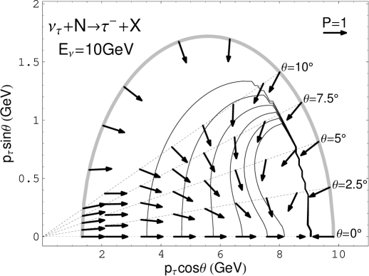
Figure 11: The contour map of the DIS cross section in the plane of $p_{\tau}\cos\theta$ and $p_{\tau}\sin\theta$ for the $\nu_{\tau}N\to\tau^{-}X$ process at $E_{\nu}=10$GeV in the laboratory frame. The kinematical boundary is shown by the thick grey curve. The QE process contributes along the boundary, and the RES process contributes just inside of the boundary. The $\tau^{-}$ polarization are shown by the arrows. The length of the arrows give the degree of polarization, and the direction of arrows give that of the $\tau^{-}$ spin in the $\tau^{-}$ rest frame. The size of the 100% polarization ($P=1$) arrow is shown as a reference. The arrows are shown along the laboratory scattering angles, $\theta=0^{\circ}$, $2.5^{\circ}$, $5^{\circ}$, $7.5^{\circ}$, and $10^{\circ}$, as well as along the kinematical boundary.

Figure 12: The same as Fig.11, but for $\bar{\nu}_{\tau}N\to\tau^{+}X$ case.

Acknowledgments

We are grateful to E.A.Paschos for useful comments and discussions. K.M. and H.Y. thank KEK theory group for the hospitality, where parts of this work were performed. K.M. would like to thank T.Morii and S.Oyama for discussions. H.Y. would like to thank M.Hirata, J.Kodaira for discussions, and RIKEN BNL Research Center for the hospitality where this work was finalized.

References

[1]
Super-Kamiokande Collaboration, Phys. Rev. Lett. 81(1988)1562;
ibid. 85(2000) 3999.
[2]
The ICARUS collaboration, arXiv:hep-ex0103008; see also the
ICARUS collaboration’s home page,
http://www.aquila.infn.it/icarus/.
[3]
The MINOS collaboration home page, http://www-numi.fnal.gov:8875/.
[4]
A. Rubbia, Nucl. Phys. Proc. Suppl. 91(2000)223, see also
the OPERA collaboration home page,
http://operaweb.web.cern.ch/operaweb/index.shtml.
[5]
L J. Hall and H. Murayama, Phys. Lett. B463(1999)241.
[6]
S. Jadach, Z. Was, R. Decker and J H. Kuhn, Comput. Phys. Commun.
76(1993) 361.
[7]
The J-PARC home page, http://j-parc.jp/index.html.
[8]
M. Apollonio et al., Phys. Lett. B420(1998)397;
ibid. B466(1999)415.
[9]
M. Aoki et al., Phys.Rev. D67(2003)093004,
M. Aoki, K. Hagiwara and N. Okamura, Phys. Lett. B554(2003)121.
[10]
E. A. Paschos and J. Y. Yu, Phys. Rev. D65(2002)033002.
[11]
S. Kretzer and M. H. Reno, Phys. Rev. D66(2002)113007.
[12]
C. H. Albright and C. Jarlskog, Nucl. Phys. B84(1975)467.
[13]
K. Hagiwara and D. Zeppenfeld, Nucl. Phys. B224(1986)1;
H. Murayama, K. Hagiwara and I. Watanabe, HELAS, KEK Report 91-11(1992).
[14]
C. H. Llewellyn Smith, Phys. Rep. 3(1972)261.
[15]
D. Rein and L. M. Sehgal, Ann. Phys. 133(1981)79.
[16]
E. A. Paschos, L. Pasquali and J. Y. Yu, Nucl. Phys. B588(2000)263.
[17]
P. A. Schreiner and F. Von Hippel, Nucl. Phys. B58(1973)333.
[18]
G. L. Fogli and G. Nardulli, Nucl. Phys. B160(1979)116.
[19]
L. Alvarez-Ruso, S. K. Singh and M. J. Vicente Vacas,
Phys. Rev. C57(1998)2693.
[20]
S. K. Singh, Nucl. Phys. B (Proc. Suppl.) 112(2002)77.
[21]
A. D. Martin, R. G. Roberts, W. J. Stirling and R. S. Thorne,
Eur. Phys. J. C23 (2002)73.
[22]
K. Hagiwara, K. Mawatari and H. Yokoya, Nucl. Phys. B668(2003)364.