Two-loop virtual QCD correction to the $B\rightarrow X_{s}l^{+}l^{-}$ decay

I discuss an application of numerical techniques for massive two-loop Feynman diagram evaluation to a phenomenologically very important rare decay process, $B\rightarrow X_{s}l^{+}l^{-}$. This process, currently being measured at B factories, has been calculated at two-loop level in the lower dilepton invariant mass perturbative window by a previous collaboration. We extended this result, by using numerical integration methods, to the whole observable spectrum of the dilepton invariant mass consistent with the perturbative QCD regime.

1 Introduction

B factories are opening the way to a class of precision electroweak measurements, including rare decays such as $B\rightarrow X_{s}l^{+}l^{-}$, which until very recently were beyond experimental reach. A measurement of the dilepton spectrum in this decay process has been proposed as a way to test for new physics and for discriminating between new physics scenarios. Even though the energy scale of this decay process is much lower than the mass scale of the new physics being tested for, and therefore these additional heavy degrees of freedom only appear as virtual effects, the $B\rightarrow X_{s}l^{+}l^{-}$ decay is relatively sensitive to them because its leading order is one-loop.

This type of analysis relies both on an accurate measurement of the dilepton spectrum, which is a matter of high integrated luminosity, and on an accurate theoretical treatment of this process. Currently, the Monte Carlo simulators in use rely on leading order calculations. One ingredient of an improved theoretical analysis is a calculation of two-loop QCD radiative corrections; this will become increasingly necessary in the future, as the integrated luminosity increases.

However, to calculate the two-loop QCD radiative corrections to this process turns out to be a difficult task. For a concise review of the theoretical effective Lagrangian framework involved, see for instance ref. 1. The Bremsstrahlung process was recently calculated in refs. 1 and 2. In their pioneering work of ref. 3, Asatryan et al. succeeded to calculate a mass and momentum double expansion of the virtual two-loop corrections for this decay process. Because their calculation is based on expansion techniques, this is a calculation of the lower dilepton spectrum perturbative window. Once the $c\bar{c}$ threshold is reached, the momentum expansion is not a valid approximation anymore.

We have recently extended this calculation to the upper perturbative window – see ref. 4. We stress that experimentally this is an important kinematic zone where a comparable number of events are collected as in the lower perturbative window; however, one encounters nonperturbative corrections in this region. To do this, we resorted to numerical methods which are valid both below and above the threshold. Regarding the lower perturbative window, our calculation serves as an independent confirmation of ref. 3, which is particularly welcome in view of the complexity of this calculation and of the fact that ref. 3 works in the mass and momentum expansion approximation. We found good agreement with Asatryan et al. at low dilepton invariant mass, while extending the result above the threshold. A detailed description of the calculation, the inclusion of the available Bremsstrahlung along with the virtual corrections, and a phenomenological analysis of the results, will be reported in ref. 4. Here we describe the calculation of the virtual QCD corrections.

2 The calculation

The relevant two-loop Feynman diagrams are shown in figure 1 . They can be organized in five gauge invariant subsets. This is useful because gauge cancellations occur within each subgroup, and gauge invariance for each subset is a useful check on the calculation.

As a first step toward the calculation of these diagrams, they are processed with a computer algebra program. We used two independent versions written in FORM and in Schoonship, which provides a powerful check on the algebra. The aim of the algebraic manipulations is to reduce the diagrams to a standard form which can be further integrated numerically. The steps involved are the Dirac algebra, introducing Feynman parameters to write the diagrams as multiple integrals over sunset-type tensor functions, Lorentz decomposition of the tensor structures and isolation of the scalar integrals, and use of differential recursion relations to reduce the scalar functions to a set of ten master scalar functions – see ref. 5. As detailed in ref. 5, the crucial point here is that any two-loop diagram in renormalizable theories can be decomposed by this algorithm into an expression involving only this limited set of ten scalar integrals. This makes this algorithm applicable, given enough computing power, to any two-loop process (up to possible infrared issues which, when manageable, must be handled analytically by hand).

After this algebra step, the Feynman diagrams are expressed as multiple integrals over a set of ten functions $h_{i}$ (or possibly their derivatives), where $h_{i}$ are the UV finite parts of a set of sunset-type scalar functions. If we denote the three propagator masses of the sunset-type functions by $m_{1}$, $m_{2}$, and $m_{3}$, and the external momentum by $k$, the ten scalar functions $h_{i}$ are defined by the following integral representations:

$$h_{1}(m_{1},m_{2},m_{3};k^{2}) = \int_{0}^{1}dx\,\tilde{g}(x)$$

$$h_{2}(m_{1},m_{2},m_{3};k^{2}) = \int_{0}^{1}dx\,[\tilde{g}(x)+\tilde{f_{1}}(x)]$$

$$h_{3}(m_{1},m_{2},m_{3};k^{2}) = \int_{0}^{1}dx\,[\tilde{g}(x)+\tilde{f_{1}}(x)]\,(1-x)$$

$$h_{4}(m_{1},m_{2},m_{3};k^{2}) = \int_{0}^{1}dx\,[\tilde{g}(x)+\tilde{f_{1}}(x)+\tilde{f_{2}}(x)]$$

$$h_{5}(m_{1},m_{2},m_{3};k^{2}) = \int_{0}^{1}dx\,[\tilde{g}(x)+\tilde{f_{1}}(x)+\tilde{f_{2}}(x)]\,(1-x)$$

$$h_{6}(m_{1},m_{2},m_{3};k^{2}) = \int_{0}^{1}dx\,[\tilde{g}(x)+\tilde{f_{1}}(x)+\tilde{f_{2}}(x)]\,(1-x)^{2}$$

$$h_{7}(m_{1},m_{2},m_{3};k^{2}) = \int_{0}^{1}dx\,[\tilde{g}(x)+\tilde{f_{1}}(x)+\tilde{f_{2}}(x)+\tilde{f_{3}}(x)]$$

$$h_{8}(m_{1},m_{2},m_{3};k^{2}) = \int_{0}^{1}dx\,[\tilde{g}(x)+\tilde{f_{1}}(x)+\tilde{f_{2}}(x)+\tilde{f_{3}}(x)]\,(1-x)$$

$$h_{9}(m_{1},m_{2},m_{3};k^{2}) = \int_{0}^{1}dx\,[\tilde{g}(x)+\tilde{f_{1}}(x)+\tilde{f_{2}}(x)+\tilde{f_{3}}(x)]\,(1-x)^{2}$$

$$h_{10}(m_{1},m_{2},m_{3};k^{2}) = \int_{0}^{1}dx\,[\tilde{g}(x)+\tilde{f_{1}}(x)+\tilde{f_{2}}(x)+\tilde{f_{3}}(x)]\,(1-x)^{3}\;\;.$$ (1)

where we used the following notations:

$$\tilde{g}(m_{1},m_{2},m_{3};k^{2};x) = Sp(\frac{1}{1-y_{1}})+Sp(\frac{1}{1-y_{2}})+y_{1}\log{\frac{y_{1}}{y_{1}-1}}+y_{2}\log{\frac{y_{2}}{y_{2}-1}}$$

$$\tilde{f_{1}}(m_{1},m_{2},m_{3};k^{2};x) = \frac{1}{2}\left[-\frac{1-\mu^{2}}{\kappa^{2}}+y_{1}^{2}\log{\frac{y_{1}}{y_{1}-1}}+y_{2}^{2}\log{\frac{y_{2}}{y_{2}-1}}\right]$$

$$\tilde{f_{2}}(m_{1},m_{2},m_{3};k^{2};x) = \frac{1}{3}\left[-\frac{2}{\kappa^{2}}-\frac{1-\mu^{2}}{2\kappa^{2}}-\left(\frac{1-\mu^{2}}{\kappa^{2}}\right)^{2}\right.$$

$$\;\;\;\;\;\;\;\;\;\;\;\;\;\;\;\;\;\;\;\;\;\;\;\;\;\;\;\;\;\;\;\;\;\;\;\;\left.+y_{1}^{3}\log{\frac{y_{1}}{y_{1}-1}}+y_{2}^{3}\log{\frac{y_{2}}{y_{2}-1}}\right]$$

$$\tilde{f_{3}}(m_{1},m_{2},m_{3};k^{2};x) = \frac{1}{4}\left[-\frac{4}{\kappa^{2}}-\left(\frac{1}{3}+\frac{3}{\kappa^{2}}\right)\left(\frac{1-\mu^{2}}{\kappa^{2}}\right)-\frac{1}{2}\left(\frac{1-\mu^{2}}{\kappa^{2}}\right)^{2}-\left(\frac{1-\mu^{2}}{\kappa^{2}}\right)^{3}\right.$$ (2)

$$\left.\;\;\;\;\;\;\;\;\;\;\;\;\;\;\;\;\;\;\;\;\;\;\;\;\;\;\;\;\;\;\;\;\;\;\;\;+y_{1}^{4}\log{\frac{y_{1}}{y_{1}-1}}+y_{2}^{4}\log{\frac{y_{2}}{y_{2}-1}}\right]\;\;,$$

$$y_{1,2} = \frac{1+\kappa^{2}-\mu^{2}\pm\sqrt{\Delta}}{2\kappa^{2}}$$

$$\Delta = (1+\kappa^{2}-\mu^{2})^{2}+4\kappa^{2}\mu^{2}-4i\kappa^{2}\eta\;\;,$$ (3)

$$\mu^{2} = \frac{ax+b(1-x)}{x(1-x)}$$

$$a = \frac{m_{2}^{2}}{m_{1}^{2}}\,,\;\;\;\;b\;=\;\frac{m_{3}^{2}}{m_{1}^{2}}\,,\;\;\;\;\kappa^{2}\;=\;\frac{k^{2}}{m_{1}^{2}}\;\;.$$ (4)

a)

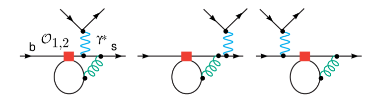
b)

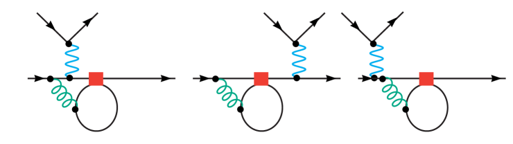
c)

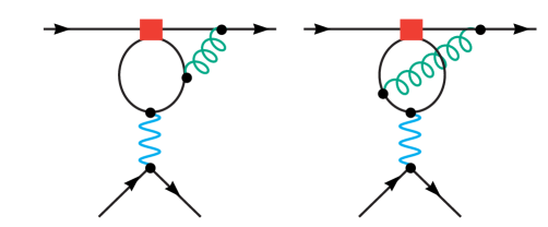
d)

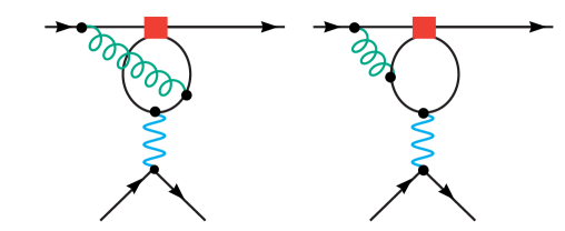
e)

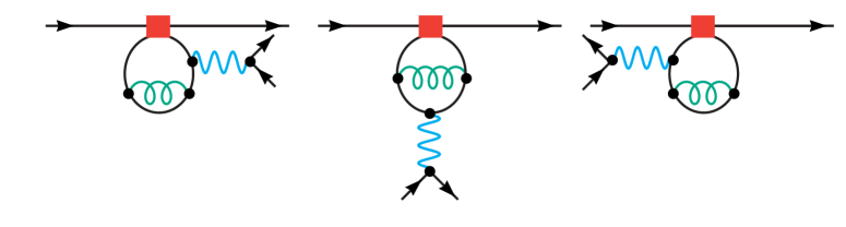
Figure 1: Two-loop Feynman diagrams relevant for the virtual QCD corrections to the rare decay $B\rightarrow X_{s}l^{+}l^{-}$. They can be organized in five gauge invariant subsets.

Figure 2: Plots of the UV finite part of the Feynman diagram subsets shown in figure 1. The two columns correspond to the electric and the magnetic form factors. We plot the real and the imaginary parts of our exact numerical integration result, along with successive approximations in the momentum expansion series of the result of Asatryan et al. which is shown only below the $c\bar{c}$ threshold.

Figure 3: Convergence pattern of the momentum expansion solution of Asatryan et al. toward our numerical integration solution. The stars denote actual integration points, and the solid line connecting them is an interpolation.

The analytical expressions that result after this first step need to be further integrated numerically. We use an adaptive deterministic integration algorithm, which is well suited for accurate numerical integrations when the dimensionality of the integral is not too large. In the problem at hand, we deal with three-fold numerical integrations at most. We note that four-fold numerical integrations were also shown to be feasible within the context of our two-loop numerical techniques in ref. 6. Based on the computing time that the four-fold integrations take, it appears likely that in the case of two-loop topologies more complicated than three-point functions, where numerical integration of higher dimensionality than four may occur, it will become more practical to use other numerical integration methods that become superior in higher dimensions, such as number-theoretical integration methods.

In general, the integrals over Feynman parameters must be performed along a complex integration path that is consistent with the causality condition. This path is computed automatically, by using spline functions. We refer to refs. 5—7 for details about the numerical integration.

In the case of the $b\rightarrow sl^{+}l^{-}$ decay, we deal with three kinematic variables: the charm mass, the dilepton invariant mass, and the subtraction scale, all normalized by the mass of the bottom quark. In order for the result to be usable for phenomenological studies, in particular to be implemented in a Monte Carlo simulation, we need to cover this three dimensional kinematic space. The actual calculation of the two-loop matrix element by numerical integration is far too slow to be implemented directly into a Monte Carlo simulation of the experimental setup. Therefore, a practical solution is to set up a suitable grid of points that cover the whole three dimensional kinematic range, and to interpolate between the points. This results into a fast program that calculates the two-loop matrix element, and which is fast enough to be included into a Monte Carlo simulation.

We selected a grid of $38\times 3\times 3$ integration points for both the electric and the magnetic components of the two-loop virtual correction. This leads to 684 integration points for the form factors involved in this calculation (see ref. 4). Each integration point was calculated with a relative precision of $10^{-3}$. We used the CERN Linux cluster to perform this calculation, and the CPU usage was approximately 3 days on 33 processors (mostly 850 MHz) running in parallel. It is obvious that with the present-day processors, calculating in advance a comprehensive grid of integration points, storing them, and then interpolating between them is the practical way to calculate such radiative corrections efficiently.

3 Results

In figure 2 we show the results for each of the five gauge invariant diagram subsets. We show both our results, valid over the whole range of the dilepton invariant mass, compared to the results of Asatryan et al., valid in principle only below the $c\bar{c}$ threshold. In figure 3 we compare the way how the momentum expansion converges toward our exact numerical solution .

There is good agreement between our results for each diagram set and the double expansion, which provides a strong test of our solution. One notices that, as a general rule, the less singular the threshold behaviour of the diagram, the better the momentum expansion converges toward our exact numerical result. In the case of the gauge invariant subset e) we notice the poorest convergence of the momentum expansion. This is correlated with the singular behaviour of this function at threshold. We note in passing that this singular behaviour is due chiefly to the charm self-energy type diagrams; this singularity is subsequently canceled when the counterterm contribution to the charm self-energy is added. This makes the agreement between our final physical result for the radiative corrections and the momentum expansion result to be better than what can be inferred from figure 3 alone.

4 Conclusions

To conclude, we calculated the virtual two-loop QCD corrections to the rare decay process $B\rightarrow X_{s}l^{+}l^{-}$. Our calculation is valid over the whole dilepton spectrum that is observable, over both the lower and the upper perturbative windows separated by the $c\bar{c}$ resonance zone. In the low dilepton invariant mass limit, we found very good agreement with an existing result by Asatryan et al., which resorts to a double expansion in the dilepton invariant mass and in the charm mass. This provides a powerful check of our result. The complete NNLO QCD effect, which includes the Bremsstrahlung along with the virtual corrections, and the phenomenological implications of these QCD corrections, will be discussed in a forthcoming article [4].

References

References

- [1] A. Ghinculov, T. Hurth, G. Isidori, Y.-P. Yao, Nucl. Phys. B 648, 254 (2003).
- [2] H.M. Asatrian, K. Bieri, C. Greub, A. Hovhannisyan, Phys. Rev. D 66, 094013 (2002).
- [3] H.H. Asatrian, H.M. Asatrian, C. Greub, M. Walker, Phys. Rev. D 65, 074004 (2002).
- [4] A. Ghinculov, T. Hurth, G. Isidori, Y.-P. Yao, in preparation; A. Ghinculov, T. Hurth, G. Isidori, Y.-P. Yao, hep-ph/0211197.
- [5] A. Ghinculov, Y.-P. Yao, Nucl. Phys. B 516, 385 (1998).
- [6] A. Ghinculov, Y.-P. Yao, Phys. Rev. D 63, 054510 (2001); A. Ghinculov, Nucl. Phys. B 455, 21 (1995).
- [7] A. Ghinculov, J.J. van der Bij, Nucl. Phys. B 436, 30 (1995); .