Theoretical determination of $\eta_{b}$’s electromagnetic decay width

Abstract

We discuss the theoretical predictions for the two photon decay width of the pseudoscalar etab meson. Predictions from potential models are examined. It is found that various models are in good agreement with each other. Results for etab are also compared with those from Upsilon data through the NRQCD procedure.

1 Introduction

First evidence of $\eta_{b}$ was given in 2001 by ALEPH [1]. The search for $\eta_{b}$ is done in the decay channel into two photons. One candidate event is found in the six–charged particle final state and none in the four–charged particle final state, giving the upper limits: $\Gamma(\eta_{b}\to\gamma\gamma)\times BR(\eta_{b}\to 4\textrm{ charged particles})<48\textrm{ eV , }$ $\Gamma(\eta_{b}\to\gamma\gamma)\times BR(\eta_{b}\to 6\textrm{ charged particles})<132\textrm{ eV .}$ This observation was the main motivation for a theoretical estimate of electromagnetic decay width for $\eta_{b}$ [2]. More recently CDF has done a search for $\eta_{b}$ in the process [3] $\eta_{b}\to J/\psi J/\psi$ with 7 events where 1.8 events are expected from background.

This note is organised as follows: in Sect. 2 we shall compare the two photon decay width with the leptonic width of the $\Upsilon$. Sect. 3 is devoted to the potential model predictions for $\eta_{b}\to\gamma\gamma$, with potential given by [5, 6, 7]. In Sect. 4 we show the predictions for $\eta_{b}$ decay widths, using the procedure introduced in [8] for the description of mesons made out of two non relativistic heavy quarks, by means of the Non Relativistic Quantum Chromodynamics–NRQCD. In Sect. 5 we compare these different determinations of the $\eta_{b}\to\gamma\gamma$ decay width together with a result based on a recent two-loop theoretical analysis of the charmonium decay [9].

2 Relation to $\Upsilon$ electromagnetic decay width

We start with the two photon decay width of a pseudoscalar quark-antiquark bound state in the singlet picture, generically written as

$$\Gamma=NP\times P$$ (1)

$NP$ being the nonperturbative part and $P$ the perturbative correction. The nonperturbative part for a state with a given $\ell$ takes the form $NP\sim|d^{\ell}\psi(0)/dr^{\ell}|^{2}$. The wavefunction is obtained by a solution of a Schrödinger equation with a suitable potential $V(r)$. The perturbative expression is given by $P=F(\alpha_{s}(m_{q}))$ and comes from the on-shell matrix element. The two photon decay width of a pseudoscalar quark-antiquark bound state [10] is given by

$$\Gamma_{B}(\eta_{b}\rightarrow\gamma\gamma)=12Q^{4}\alpha^{2}4\pi\frac{|\psi(0)|^{2}}{M^{2}}\equiv\Gamma_{B}^{P}$$ (2)

$M=2m_{b}+E_{b}$ being the mass of the state, $E_{b}$ the (negative) binding energy; with first order QCD corrections [11], which can be written as

$$\Gamma(\eta_{b}\rightarrow\gamma\gamma)=\Gamma_{B}^{P}\left[1+\frac{\alpha_{s}}{\pi}\left(\frac{\pi^{2}-20}{3}\right)\right].$$ (3)

A first theoretical estimate for this decay width can be obtained by comparing eq. (3) with the expression for the electromagnetic decay for the vector state $\Upsilon$ [12], i.e.

$$\Gamma_{B}(\Upsilon\rightarrow e^{+}e^{-})=4Q^{2}\alpha^{2}4\pi\frac{|\psi(0)|^{2}}{M^{2}}\equiv\Gamma_{B}^{V}$$ (4)

and the one-loop complete formula

$$\Gamma(\Upsilon\rightarrow e^{+}e^{-})=\Gamma_{B}^{V}\left(1-\frac{16}{3}\frac{\alpha_{s}}{\pi}\right).$$ (5)

Using the expressions in eqs. (3) and (5) we can estimate the $\eta_{b}$ decay width from the the measured values of the leptonic decay width of $\Upsilon$. We assume the wavefunctions of the two states to be equal, that leads to an error proportional to $(\alpha_{s}/m_{b}^{2})$ [2]. Taking the ratio of the eqs. (3) and (5) and expanding to first order in $\alpha_{s}$, we obtain:

$$\frac{\Gamma(\eta_{b}\rightarrow\gamma\gamma)}{\Gamma(\Upsilon\rightarrow e^{+}e^{-})}\approx\frac{1}{3}\frac{(1-3.38\alpha_{s}/\pi)}{(1-5.34\alpha_{s}/\pi)}=$$

$$=\frac{1}{3}\left[1+1.96\frac{\alpha_{s}}{\pi}+\mathcal{O}(\alpha_{s}^{2})\right].$$ (6)

In order to compute the correction we start from the two-loop expression for $\alpha_{s}$ and the value at the $Z$ mass [15] $\alpha_{s}(M_{Z})=0.118\pm 0.003$. Using the renormalization group equation to evaluate $\alpha_{s}(Q=2m_{b}=10.0\mbox{ GeV})=0.178\pm 0.007$, and the latest measurement of the $\Upsilon$

$$\Gamma_{exp}(\Upsilon\to e^{+}e^{-})=1.32\pm 0.05\textrm{ keV }$$ (7)

for the $\eta_{b}$ one obtains

$$\Gamma(\eta_{b}\rightarrow\gamma\gamma)\pm\Delta\Gamma(\eta_{b}\rightarrow\gamma\gamma)=489\pm 19\pm 2\textrm{ eV ,}$$ (8)

where the first error comes from the uncertainty on the $\Upsilon$ experimental width, the second error from $\alpha_{s}$ . We have assumed the $\alpha_{s}$ scale to be $Q=2m_{b}=10.0\textrm{ GeV}$. This choice is by no way unique as shown for the $\eta_{c}$ decay [4], and in fig. (1) we show the dependence of the $\eta_{b}$ photonic width, evaluated from eq. (7), upon different values of the scale chosen for $\alpha_{s}$ .

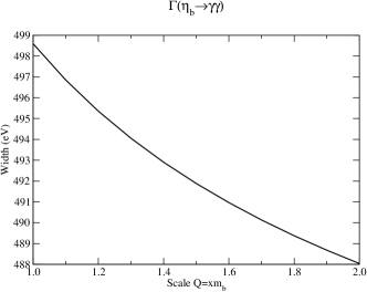
Figure 1: The dependence of the $\eta_{b}$ decay width to $\gamma\gamma$ (in eV) is shown with respect to the scale chosen for $\alpha_{s}$ in the radiative corrections. The fluctuation is of order 2%

Unlike the $\eta_{c}$ case there are no experimental measurements of this decay; we shall assume therefore that it is not possible to determine a scale choice of $\alpha_{s}$ for the $\eta_{b}$ decay. We will have to include this fluctuation in the indetermination due to radiative corrections.

3 Potential Model predictions

We present now results for $\eta_{b}\to\gamma\gamma$ from the potential models. This method allows us to obtain the absolute width, through the wave function at the origin computed from a Schrödinger equation. For the calculation of the wavefunction [16] we have used four different potential models, starting from the one of Rosner et al. [5] $V(r)=\lambda((r/r_{0})^{\alpha}-1)/\alpha+C\mbox{ .}$ with $r_{0}=1\textrm{ GeV}^{-1},\;\alpha=-0.14\mbox{ , }\lambda=0.808\textrm{ GeV, }C=-1.305\textrm{ GeV}$, and the QCD inspired potential $V_{J}$ of Igi-Ono [6, 17]

$$V_{J}(r)=V_{AR}(r)+dre^{-gr}+ar,$$

$$V_{AR}(r)=-\frac{4}{3}\frac{\alpha_{s}^{(2)}(r)}{r}$$ (9)

with two different parameter sets, corresponding to $\Lambda_{\overline{MS}}=0.5\ GeV$ and $\Lambda_{\overline{MS}}=0.2\ GeV$ respectively [6]. We show also the results from a Coulombic type potential with the QCD coupling $\alpha_{s}$ frozen to a value of $r$ which corresponds to the Bohr radius of the quarkonium system, $r_{B}=3/(2m_{b}\alpha_{s}(r_{B}))$ (see for instance [7]). The latter has the advantage of providing analytical solutions for the wavefunction and the energy levels: $E_{n}=-4m\alpha_{s}(r_{B})^{2}/(9n^{2})$ and $|\psi(0)|^{2}=(2m\alpha_{s}(r_{B})/3)^{3}/\pi$

We have to stress the fact that the scale of $\alpha_{s}$ occurring in the radiative correction and the one of Coulombic potential are different. We show in fig. (2) the predictions for the decay width from these potential models with the correction from eq. (3) at an $\alpha_{s}$ scale $Q=2m_{b}$ .

Figure 2: The dependence of $\eta_{b}$ decay width to $\gamma\gamma$ in eV for different potential models is shown as a function of $m_{b}$. The perturbative correction scale is here set to be $Q=2m_{b}$.

For any given model, sources of error in this calculation arise from the choice of scale in the radiative correction factor discussed before and the choice of the parameters. The difference of the prediction between the various models introduce another indetermination for the decay value. We can estimate a range of values for the potential model predictions for the radiative decay width $\Gamma(\eta_{b}\to\gamma\gamma)$, namely:

$$\Gamma(\eta_{b}\to\gamma\gamma)=466\pm 101\textrm{ eV \mbox{ },}$$ (10)

that is an indetermination of around 22%.

4 Octet component procedure

We will present now another approach which admits other components to the meson decay beyond the one from the colour singlet picture (Bodwin, Braaten and Lepage) [8]. NRQCD has been used to separate the short distance scale of annihilation from the nonperturbative contributions of long distance scale. This model has been successfully used to explain the larger than expected $J/\psi$ production at the Tevatron and LEP. The decay width expression for a pseudoscalar $P$ or a vector state $V$ is given by means of NRQCD from the expansion:

$$\Gamma_{V,P}=\sum_{n}\frac{2\Im f_{n}(\alpha_{s})}{m_{q}^{d{{}_{n}}-4}}\langle\mathcal{O}_{n}\rangle_{V,P}$$ (11)

that is a sum of terms in inverse powers of $m_{q}$, each of which factorises into a perturbative coefficient $\Im f_{n}(\alpha_{s})$ and nonperturbative matrix element $\langle\mathcal{O}_{n}\rangle_{V,P}$.

According to BBL, in the octet model for quarkonium, the electromagnetic and light hadrons ($LH$) decay widths of bottomonium states are given by:

$$\Gamma(\Upsilon\to LH)=\frac{2\langle\Upsilon|O_{1}(^{3}S_{1})|\Upsilon\rangle}{m_{b}^{2}}\left(\frac{10}{243}\pi^{2}-\frac{10}{27}\right)\alpha_{s}^{3}$$

$$\times\left[1+\left(-9.46\times\frac{4}{3}+12.39-1.161n_{f}\right)\frac{\alpha_{s}}{\pi}\right]+$$

$$\frac{2\langle\Upsilon|P_{1}(^{3}S_{1})|\Upsilon\rangle}{m_{b}^{4}}\frac{17.32\times\left[20(\pi^{2}-9)\right]}{486}\alpha_{s}^{3}$$ (12)

$$\Gamma(\Upsilon\to e^{+}e^{-})=\frac{2\langle\Upsilon|O_{1}(^{3}S_{1})|\Upsilon\rangle}{m_{b}^{2}}\left[\frac{\pi}{3}Q^{2}\alpha^{2}\left(1-\right.\right.$$

$$\left.\left.\frac{13}{3}\frac{\alpha_{s}}{\pi}\right)\right]-\frac{2\langle\Upsilon|P_{1}(^{3}S_{1})|\Upsilon\rangle}{m_{b}^{4}}\frac{4}{9}\pi Q^{2}\alpha^{2}$$ (13)

$$\Gamma(\eta_{b}\to LH)=\frac{2\langle\eta_{b}|O_{1}(^{1}S_{0})|\eta_{b}\rangle}{m_{b}^{2}}\frac{2}{9}\pi\alpha_{s}^{2}\left[1+\left(\frac{53}{2}\right.\right.$$

$$\left.\left.-\frac{31}{24}\pi^{2}-\frac{8}{9}n_{f}\right)\right]-\frac{2\langle\eta_{b}|P_{1}(^{1}S_{0})|\eta_{b}\rangle}{m_{b}^{4}}\frac{8}{27}\pi\alpha_{s}^{2}$$ (14)

$$\Gamma(\eta_{b}\to\gamma\gamma)=\frac{2\langle\eta_{b}|O_{1}(^{1}S_{0})|\eta_{b}\rangle}{m_{b}^{2}}\pi Q^{4}\alpha^{2}\left[1+\right.$$

$$\left.\left(\frac{\pi^{2}-20}{3}\right)\frac{\alpha_{s}}{\pi}\right]-\frac{2\langle\eta_{b}|P_{1}(^{1}S_{0})|\eta_{b}\rangle}{m_{b}^{4}}\frac{4}{3}\pi Q^{4}\alpha^{2}$$ (15)

There are four unknown long distance coefficients, which can be reduced to two by means of the vacuum saturation approximation:

$$G_{1}\equiv\langle\Upsilon|O_{1}(^{3}S_{1})|\Upsilon\rangle=\langle\eta_{b}|O_{1}(^{1}S_{0})|\eta_{b}\rangle$$ (16)

$$F_{1}\equiv\langle\Upsilon|P_{1}(^{3}S_{1})|\Upsilon\rangle=\langle\eta_{b}|P_{1}(^{1}S_{0})|\eta_{b}\rangle$$ (17)

which is correct up to $\mathcal{O}(v^{2})$, where ${\vec{v}}$ is the quark velocity inside the meson. In the potential model language this translates to consider the two wavefunctions of the pseudoscalar and the vector state to be equal. With this position we obtain a system of equations for the nonperturbative coefficients $G_{1}$ and $F_{1}$ of $\Upsilon$ electromagnetic decay and light hadrons widths which in turn allows us to compute the $\eta_{b}$ decay widths.

The BBL approach gives the following decay widths of the $\eta_{b}$ meson:

$$\Gamma(\eta_{b}\rightarrow\gamma\gamma)=364\pm 8\pm 13\textrm{ eV}$$ (18)

and

$$\Gamma(\eta_{b}\rightarrow LH)=57.9\pm 4.6\pm 2.8\textrm{ keV ,}$$ (19)

where the first error comes from the uncertainty on the $\Upsilon$ experimental width, the second error from $\alpha_{s}$ . The improvement of the error on eq. (18) with respect to the previous analogous determination on the $\eta_{c}$ decay [4] is due to better error on the experimental measures of the $\Upsilon$ decay widths compared to the one of the $J/\psi$, and the smaller indetermination on the $\alpha_{s}$ value due to the higher energy scale involved in the decay. These reasons, together with the fact that the potential models used are fitted for the $c\overline{c}$ system, justifies the improvement of accuracy given in eq. (18) compared to the one of eq. (10).

5 Comparison between models

For comparison we present in fig. (3) a set of predictions coming from different methods.

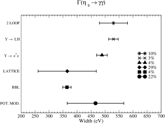
Figure 3: The $\eta_{b}$ two photon width as calculated in this paper using (starting from below) Potential Models results, BBL procedure with input from $J/\psi$ decay data, Lattice evaluation of $G_{1}$ and $F_{1}$ factors, Singlet picture with $G_{1}$ obtained from $\Upsilon\to e^{+}e^{-}$ and $\Upsilon\to LH$ processes respectively, and the two–loop enhanced procedure. The legend shows the percentage error on each value.

Starting with potential models, we see that the results are in good agreement with each other. The advantage of this method is that we are giving a prediction from first principles, without using any experimental input. Since there are currently no experimental measures for the $\eta_{b}\to\gamma\gamma$ decay, we shall use this prediction as a reference point, as it has proven to be reliable in the case of charmonium decay [4]. The second evaluation, given by BBL using the experimental values of the $\Upsilon$ decay, is on the left limit of the potential models value. This is true also for the determination of the BBL procedure with nonperturbative long distance terms taken from from the lattice calculation [18], affected from a large error of around 30%. The advantage of the latter is that its prediction, like the one from potential models, does not make use of any experimental value. Next is the point given by the singlet picture from the electromagnetic decay of the $\Upsilon$, aligned with the aforementioned results of the BBL procedure. The point above is obtained also from the singlet picture with the $\Upsilon$ decay into light hadrons, in agreement with the results given from the potential models. We notice that in analogy to the charmonium case (see [4] and references therein) the singlet results obtained from the $\Upsilon$ decay are in disagreement with each other, in this case by only $1\sigma$. The last point from a two–loop enhanced calculation given by [9, 1] is in agreement with the potential model result and the singlet decay from the $\Upsilon\to LH$ process.

6 Conclusions

The $\Gamma(\eta_{b}\to\gamma\gamma)$ decay width prediction of the potential models considered gives the value $466\pm 101\textrm{ eV}$, in agreement with the naive estimate from the $\Upsilon$ decay given by (8). Predictions of the BBL procedure are consistent with the potential model results, for both the long distance terms $G_{1}$ and $F_{1}$ extracted from the $\Upsilon$ experimental decay widths and the one evaluated from lattice calculations. The results from the singlet picture are also consistent with the potential model results. Finally the two–loop enhanced prediction is in good agreement with the potential model results.

References

- [1] A. Böhrer, hep-ph/0110030, to appear in proceedings of “PHOTON 2001”, Ascona, Switzerland (2001), ed. by M. Kienzle, World Sci., Singapore, 2001, and private communication; The ALEPH Collaboration, A. Heister et al., Phys. Lett.B 530 (2002) 56.
- [2] Nicola Fabiano Eur. Phys. J. C26 (2003) 441-444; N. Fabiano , G. Pancheri, To appear in the proceedings of “1st International Workshop on Frontier Science: Charm, Beauty, and CP”, Frascati, Rome, Italy, 6-11 Oct 2002. e-Print Archive: hep-ph/0210279.
- [3] CDF Collaboration (J. Tseng for the collaboration), FERMILAB-Conf-02/348-E.
- [4] N. Fabiano, G. Pancheri, hep-ph/0110211, to appear in proceedings of “PHOTON 2001”, Ascona, Switzerland (2001), ed. by M. Kienzle, World Sci., Singapore, 2001; N. Fabiano, G. Pancheri, Eur. Phys. J. C25 (2002) 421.
- [5] A.K. Grant, J.L. Rosner and E. Rynes, Phys. Rev. D47 (1993) 1981.
- [6] J. H. Kühn and S. Ono, Zeit. Phys.C21 (1984) 385; K. Igi and S. Ono, Phys. Rev. D33 (1986) 3349.
- [7] N. Fabiano, A. Grau and G. Pancheri, Phys. Rev. D50 (1994) 3173; Nuovo Cimento A, Vol 107 (1994) 2789.
- [8] G.T. Bodwin, E. Braaten and G.P. Lepage, Phys. Rev. D51 (1995) 1125.
- [9] A. Czarnecki and K. Melnikov, Phys. Lett.B 519 (2001) 212.
- [10] R.Van Royen and V.Weisskopf, Nuovo Cimento 50A (1967) 617.
- [11] R. Barbieri, G. Curci, E. d’Emilio and R. Remiddi Nucl. Phys. B154 (1979) 535.
- [12] P. Mackenzie and G. Lepage, Phys. Rev. Lett.47 (1981) 1244.
- [13] E. Eichten, K. Gottfried, T. Kinoshita, K. D. Lane and T. M. Yan, Phys. Rev. 21D (1980) 203.
- [14] E. Eichten and F. Feinberg, Phys. Rev. D23, (1981) 2724.
- [15] Review of Particle Properties, K. Hagiwara et al., Phys. Rev. D66, (2002) 010001; http://pdg.lbl.gov/.
- [16] Thanks to F.F. Schöbrl for providing the program; W. Lucha, F.F. Schöbrl, Int. J. Mod. Phys. C 10 (1999) 607.
- [17] W. Buchmuller and S. H. H. Tye, Phys. Rev. D24 (1981) 132.
- [18] G.T. Bodwin, D.K. Sinclair and S. Kim, Int. J. Mod. Phys. A 999 (2001) 123.