Domain wall generation by fermion self-interaction and light particles

Abstract:

A possible explanation for the appearance of light fermions and Higgs bosons on the four-dimensional domain wall is proposed. The mechanism of light particle trapping is accounted for by a strong self-interaction of five-dimensional pre-quarks. We obtain the low-energy effective action which exhibits the invariance under the so called $\tau$-symmetry. Then we find a set of vacuum solutions which break that symmetry and the five-dimensional translational invariance. One type of those vacuum solutions gives rise to the domain wall formation with consequent trapping of light massive fermions and Higgs-like bosons as well as massless sterile scalars, the so-called branons. The induced relations between low-energy couplings for Yukawa and scalar field interactions allow to make certain predictions for light particle masses and couplings themselves, which might provide a signature of the higher dimensional origin of particle physics at future experiments. The manifest translational symmetry breaking, eventually due to some gravitational and/or matter fields in five dimensions, is effectively realized with the help of background scalar defects. As a result the branons acquire masses, whereas the ratio of Higgs and fermion (presumably top-quark) masses can be reduced towards the values compatible with the present-day phenomenology. Since the branons do not couple to fermions and the Higgs bosons do not decay into branons, the latter ones are essentially sterile and stable, what makes them the natural candidates for the dark matter in the Universe.

1 Introduction

The accommodation of our matter world on a four-dimensional surface – a domain wall or a thick 3-brane – in a multi-dimensional space-time with dimension higher than four has recently attracted much interest as a theoretical concept [1]-[6] promoting novel solutions to the long standing problems of the Planck mass scale [3, 4], GUT scale [7, 8], SUSY breaking scale [9, 10], electroweak breaking scale [11]-[14] and fermion mass hierarchy [15, 16]. Respectively, an experimental challenge has been posed for the forthcoming collider and non-collider physics programs to discover new particles, such as Kaluza-Klein gravitons [18, 19], radions and graviscalars [20, 21], branons [22]-[24], sterile neutrinos [7, 25, 26, 27] etc., together with some other missing energy [28] or missing charge effects [29]. The vast literature on those subjects and their applications is now covered in few review articles [30]-[35]. Typically, the thick or fat domain wall formation and the trapping of low-energy particles on its surface (layer) might be obtained [36]-[38] by a number of particular background scalar and/or gravitational fields living in the multi-dimensional bulk – see however Ref. [39] – the configuration of which does generate zero-energy states localized on the brane. Obviously, the explanation of how such background fields can emerge and induce the spontaneous symmetry breaking is to be found and the domain wall creation, due to self-interaction of certain particles in the bulk with low-energy counterparts populating our world, may be one conceivable possibility.

In this paper we consider and explore the non-compact 4 + 1-dimensional fermion model with strong local four-fermion interaction that leads to the discrete symmetry breaking, owing to which the domain wall pattern of the vacuum state just arises and allows the light massive Dirac particles to live in four dimensions. In such a model the scalar fields appear to be as composite ones. We are aware of the possible important role [31, 37] of a non-trivial gravitational background, of propagating gravitons and gauge fields for issues of stability of the domain wall induced by a fermion self-interaction. Nonetheless, in order to keep track of the main dynamical mechanism, we simplify herein the fermion model just neglecting all gravitational and gauge field interaction and, in this sense, our model might be thought as a sector of the full Domain-Wall Standard Model. However, we believe that the simplified model we treat in the present investigation will be able to give us the plenty of quantitative hints on the relationships among physical characteristics of light particles trapped on the brane.

Let us elucidate the domain wall phenomenology in more details and start from the model of one five-dimensional fermion bi-spinor $\psi(X)$ coupled to a scalar field $\Phi(X)$. The extra-dimension coordinate is assumed to be space-like,

$$(X_{\alpha})=(x_{\mu},z)\ ,\quad(x_{\mu})=(x_{0},x_{1},x_{2},x_{3})\ ,\quad(g_{\alpha\alpha})=(+,-,-,-,-)$$

and the subspace of $x_{\mu}$ eventually corresponds to the four-dimensional Minkowski space. The extra-dimension size is supposed to be infinite (or large enough). The fermion wave function is then described by the Dirac equation

$$[\,i\gamma_{\alpha}\partial^{\alpha}-\Phi(X)\,]\psi(X)=0\ ,\quad\gamma_{\alpha}=(\gamma_{\mu},-i\gamma_{5})\ ,\quad\{\gamma_{\alpha},\gamma_{\beta}\}=2g_{\alpha\beta}\ ,$$ (1)

with $\gamma_{\alpha}$ being a set of four-dimensional Dirac matrices in the chiral representation.

The trapping of light fermions on a four-dimensional hyper-plane – the domain wall – localized in the fifth dimension at $z=z_{0}$ can be promoted by a certain topological, $z$-dependent background configuration of the scalar field $\langle\Phi(X)\rangle_{0}=\varphi(z)$, due to the appearance of zero-modes in the four-dimensional fermion spectrum. In this case, from the viewpoint of four-dimensional space-time, Eq. (1) just characterizes the infinite set of fermions with different masses that it is easier to see after the Fock-Schwinger transformation,

$$[\,i\gamma_{\alpha}\partial^{\alpha}+\varphi(z)\,][\,i\gamma_{\alpha}\partial^{\alpha}-\varphi(z)\,]\psi(X)\equiv(-\partial_{\mu}\partial^{\mu}-\widehat{m}^{2}_{z})\psi(X)\ ;$$

$$\widehat{m}^{2}_{z}=-\partial_{z}^{2}+\varphi^{2}(z)-\gamma_{5}\varphi^{\prime}(z)=\widehat{m}^{2}_{+}P_{L}+\widehat{m}^{2}_{-}P_{R}\ ,$$ (2)

where $P_{L,R}=\frac{1}{2}(1\pm\gamma_{5})$ are projectors on the left- and right-handed states. Thus the mass operator consists of two chiral superpartners – in the sense of supersymmetric quantum mechanics [43]-[45]

$$\widehat{m}_{\pm}^{2} = -\partial_{z}^{2}+\varphi^{2}(z)\mp\varphi^{\prime}(z)=[\,-\partial_{z}\pm\varphi(z)\,][\,\partial_{z}\pm\varphi(z)\,]\ ;$$ (3)

$$\widehat{m}_{+}^{2}\,q^{+} = q^{+}\,\widehat{m}_{-}^{2},\quad\widehat{m}_{-}^{2}\,q^{-}=q^{-}\,\widehat{m}_{+}^{2}\ ,\quad q^{\pm}\equiv\mp\partial_{z}+\varphi(z)\ .$$ (4)

The factorization (3) guarantees the positivity of the mass operator – i.e. the absence of tachyons – and the supersymmetry realized by the intertwining relations (4) entails the equivalence of the spectra between different chiralities for non-vanishing masses. As a consequence, the related left- and right-handed spinors can be assembled into the bi-spinor describing a massive Dirac particle which, however, is not necessarily localized at any point of the extra-dimension if the field configuration $\varphi(z)$ is asymptotically constant. Indeed the massive states will typically belong to the continuous spectrum – or to a Kaluza-Klein tower for the compact fifth dimension – and spread out the whole extra-dimension. Meanwhile, the spectral equivalence may be broken just by one single state, i.e. a proper normalizable zero mode of one of the mass operators $\widehat{m}_{\pm}^{2}$. Let us assume to get it in the spectrum of $\widehat{m}_{+}^{2}$: then from Eq.s (3) and (4) it follows that

$$q^{-}\psi^{+}_{0}(x,z)=0\ ,\quad\psi^{+}_{0}(x,z)=\psi_{L}(x)\,\exp\left\{-\int^{z}_{z_{0}}dw\varphi(w)\right\}\ ,$$ (5)

where $\psi_{L}(x)=P_{L}\psi(x)$ is a free Weyl spinor in the four-dimensional Minkowski space. Evidently, if a scalar field configuration has the following asymptotic behavior: namely,

$$\varphi(z)\stackrel{{\scriptstyle z\rightarrow\pm\infty}}{{\sim}}\pm C_{\pm}|z|^{\nu_{\pm}}\ ,\quad\mbox{\rm Re}\nu_{\pm}>-1\ ,\quad C_{\pm}>0\ ,$$

then the wave function $\psi^{+}_{0}(x,z)$ is normalizable on the $z$ axis and the corresponding left-handed fermion is a massless Weyl particle localized in the vicinity of a four-dimensional domain wall. It is easy to check that in this case the superpartner mass operator $\widehat{m}_{-}^{2}$ does not possess a massless normalizable solution and if $\varphi(z)$ is asymptotically constant, with $C_{\pm}>0$ and $\nu_{\pm}=0$, there is always a gap for the massive Dirac states. Further on we restrict ourselves to this scenario.

The important example of such a topological configuration can be derived for the system having the free mass spectrum – continuum or Kaluza-Klein tower – for one of the chiralities, say, for right-handed fermions. This is realized by a kink-like scalar field background

$$\varphi^{+}=M\,\mbox{\rm tanh}(Mz)\ .$$ (6)

The two mass operators have the following potentials

$$\widehat{m}^{2}_{+}=-\partial_{z}^{2}+M^{2}\left[\,1-2{\rm sech}^{2}(Mz)\,\right];\quad\widehat{m}^{2}_{-}=-\partial_{z}^{2}+M^{2},$$ (7)

and the left-handed normalized zero-mode is properly localized around $z=0$, in such a way that we can set

$$\psi^{+}_{0}(x,z)=\psi_{L}(x)\,\psi_{0}(z)\ ,\qquad\psi_{0}(z)\equiv\sqrt{M/2}\ {\rm sech}(Mz)\ .$$ (8)

As a consequence, the threshold for the continuum is at $M^{2}$ and the heavy Dirac particles may have any masses $m>M$, the corresponding wave-functions being completely de-localized in the extra-dimension.

On the one hand, if we investigate the scattering and decay of particles with energies considerably smaller than $M$, we never reach the threshold of creation of heavy Dirac particles with $m>M$ and all physics interplays on the four-dimensional domain wall with thickness $\sim 1/M$. On the other hand, at extremely high energies, certain heavy fermions will appear in and disappear from our world.

It turns out that the real fermions – quarks and leptons living on the domain wall by assumption – are mainly massive. Therefore, for each light fermion on a brane one needs at least two five-dimensional proto-fermions $\psi_{1}(X),\psi_{2}(X)$ in order to generate left- and right-handed parts of a four-dimensional Dirac bi-spinor as zero modes. Those fermions have clearly to couple with opposite charges to the scalar field $\Phi(X)$, in order to produce the required zero modes with different chiralities when $\langle\Phi(X)\rangle_{0}=\varphi^{+}(z)$: namely,

$$[\,i\not\!\partial-\tau_{3}\Phi(X)\,]\Psi(X)=0\ ,\quad\not\!\partial\equiv\widehat{\gamma}_{\alpha}\partial^{\alpha}\ ,\quad\Psi(X)=\left\lgroup\begin{array}[]{c}\psi_{1}(X)\\ \psi_{2}(X)\end{array}\right\rgroup\ ,$$ (9)

where $\widehat{\gamma}_{\alpha}\equiv\gamma_{\alpha}\otimes{\bf 1}_{2}$ are Dirac matrices and $\tau_{a}\equiv{\bf 1}_{4}\otimes\sigma_{a},\ a=1,2,3$ are the generalizations of the Pauli matrices $\sigma_{a}$ acting on the bi-spinor components $\psi_{i}(X)$.

In this way one obtains a massless Dirac particle on the brane and the next task is to supply it with a light mass. As the mass operator mixes left- and right-handed components of the four-dimensional fermion it is embedded in the Dirac operator (9) with the mixing matrix $\tau_{1}m_{f}$ of the fields $\psi_{1}(X)$ and $\psi_{2}(X)$. At last, following the general Standard Model mechanism of fermion mass generation by means of the Higgs scalars, one can introduce the second scalar field $H(x)$ to make this job, replacing the bare mass $\tau_{1}m_{f}\longrightarrow\tau_{1}H(x)$. Both scalar fields might be dynamical indeed and their self-interaction should justify the spontaneous symmetry breaking by certain classical configurations allocating light massive fermions on the domain wall. From the previous discussion it follows that the minimal set of five-dimensional fermions has to include two Dirac fermions coupled to scalar backgrounds of opposite signs. In addition to the trapping scalar field, another one is in order to supply light domain wall fermions with a mass. Thus we introduce two types of four-fermion self-interactions to reveal two composite scalar fields with a proper coupling to fermions. As we shall see, these two scalar fields will acquire mass spectra similar to fermions with light counterparts located on the domain wall. The dynamical mechanism of creation of domain wall particles turns out to be quite economical and few predictions on masses and decay constants of fermion and boson particles will be derived.

2 Fermion model with self-interaction in 5D

Let us consider the model with the following Lagrange density

$${\cal L}^{(5)}(\overline{\Psi},\Psi)=\overline{\Psi}\ i\!\not\!\partial\Psi+\frac{g_{1}}{4N\Lambda^{3}}\left(\overline{\Psi}\tau_{3}\Psi\right)^{2}+\frac{g_{2}}{4N\Lambda^{3}}\left(\overline{\Psi}\tau_{1}\Psi\right)^{2},$$ (10)

where $\Psi(X)$ is an eight-component five-dimensional fermion field, see Eq. (9) – either a bi-spinor in a four-dimensional theory or a spinor in a six-dimensional theory – which may also realize a flavor and color multiplet with the total number $N=N_{f}\,N_{c}$ of states. The ultraviolet cut-off scale $\Lambda$ bounds fermion momenta, as the four-fermion interaction is supposed here to be an effective one, whereas $g_{1}$ and $g_{2}$ are suitable dimensionless and eventually scale dependent effective couplings.

This Lagrange density can be more transparently treated with the help of a pair of auxiliary scalar fields $\Phi(X)$ and $H(X)$, which eventually will allow to trap a light fermion on the domain wall and to supply it with a mass

$${\cal L}^{(5)}(\overline{\Psi},\Psi,\Phi,H)=$$

$$\overline{\Psi}(i\!\not\!\partial-\tau_{3}\Phi-\tau_{1}H)\Psi-\frac{N\Lambda^{3}}{g_{1}}\,\Phi^{2}-\frac{N\Lambda^{3}}{g_{2}}\,H^{2}\ .$$ (11)

In this model the invariance (when it holds) under discrete $\tau$-symmetry transformations

$$\Psi\longrightarrow\tau_{1}\Psi\ ;\quad\Phi\longrightarrow-\,\Phi\ ;$$ (12)

$$\Psi\longrightarrow\tau_{2}\Psi\ ;\quad\Phi,H\longrightarrow-\,\Phi,-\,H\ ;$$ (13)

$$\Psi\longrightarrow\tau_{3}\Psi\ ;\quad H\longrightarrow-\,H\ ,$$ (14)

does not allow the fermions to acquire a mass and prevents a breaking of translational invariance in the perturbation theory. This $\tau$-symmetry can be associated to the chiral symmetry in four dimensions .

However for sufficiently strong couplings, this system undergoes the phase transition to the state in which the condensation of fermion-anti-fermion pairs does spontaneously break – partially or completely – the $\tau$-symmetry.

The physical meaning of the scale $\Lambda$ is that of a compositeness scale for heavy scalar bosons emerging after the breakdown of the $\tau$-symmetry. In order to develop the infrared phenomenon of $\tau$-symmetry breaking, the effective Lagrange density containing the essential low-energy degrees of freedom has to be derived.

To this concern we proceed – only in this Section – to the transition to the Euclidean space, where the invariant four-momentum cut-off can be unambiguously implemented. Within this framework, the notion of low-energy is referred to momenta $|p|<\Lambda_{0}$ as compared to the cut-off $\Lambda\gg\Lambda_{0}$. However, after the elaboration of the domain wall vacuum, we will search for the fermion states with masses $m_{f}$ much lighter than the dynamic scale $\Lambda_{0}$, i.e. for the ultralow-energy physics. Thus, eventually, there are three scales in the present model in order to implement the domain wall particle trapping.

Let us decompose the momentum space fermion fields into their high-energy part $\Psi_{h}(p)\equiv\Psi(p)\vartheta(|p|-\Lambda_{0})\vartheta(\Lambda-|p|)$, their low-energy part $\Psi_{l}(p)\equiv\Psi(p)\vartheta(\Lambda_{0}-|p|)$ and integrate out the high-energy part of the fermion spectrum, $\vartheta(t)$ being the usual Heaviside step distribution. More rigorously, the above decomposition of the fermion spectrum should be done covariantly, i.e. in terms of the full Euclidean Dirac operator,

$$D\equiv i(\not\!\partial+\tau_{3}\Phi+\tau_{1}H)\ .$$ (15)

Nevertheless, as we want to concentrate ourselves on the triggering of $\tau$-symmetry breaking by fermion condensation, we can safely assume to neglect further on the high-energy components of the auxiliary boson fields, what is equivalent to the use of the mean-field or large $N$ approximations. Then the low-energy Lagrange density, which solely accounts for low-energy fermion and boson fields, can be written as the sum of the expression in Eq. (11) and the one-loop effective Lagrange density: namely,

$${\cal L}^{(5)}_{\rm low}(\overline{\Psi}_{l},\Psi_{l},\Phi,H)={\cal L}^{(5)}_{E}(\overline{\Psi}_{l},\Psi_{l},\Phi,H)+\Delta{\cal L}^{(5)}(\Phi,H),$$ (16)

where the tree-level low-energy Euclidean Lagrange density reads

$${\cal L}^{(5)}_{E}(\overline{\Psi}_{l},\Psi_{l},\Phi,H)=i\overline{\Psi}_{l}(\!\not\!\partial+\tau_{3}\Phi+\tau_{1}H)\Psi_{l}+\frac{N\Lambda^{3}}{g_{1}}\,\Phi^{2}+\frac{N\Lambda^{3}}{g_{2}}\,H^{2}.$$ (17)

The one-loop contribution of high-energy fermions is given by

$$\Delta{\cal L}^{(5)}(\Phi,H)=C-(N/2)\,\mbox{tr}\langle X|{\rm A}|X\rangle\ ,$$ (18)

$${\rm A}\equiv\vartheta(\Lambda^{2}-D^{\dagger}D)\ln\frac{D^{\dagger}D}{\Lambda^{2}}-\vartheta(\Lambda_{0}^{2}-D^{\dagger}D)\ln\frac{D^{\dagger}D}{\Lambda_{0}^{2}}\ ,$$

where the normalization constant $C$ is such that $\Delta{\cal L}^{(5)}(0,0)=0$ and the ${\rm tr}$ operation stands for the trace over spinor and internal degrees of freedom. In Eq. (18) the choice of normalizations in the logarithms ensures the continuity of spectral density at the positions of cut-offs $\Lambda$ and $\Lambda_{0}$. Thereby the spectral flow through the spectral boundary is suppressed. In the latter operator ${\rm A}$ we have incorporated the cut-offs which select out the high-energy region defined above [46].
From the conjugation property $D^{\dagger}=\tau_{2}D\tau_{2}$, it follows that the Euclidean Dirac operator is a normal operator, which has to be implemented in order to get a real effective action and to define the spectral cut-offs with the help of the positive operator

$$D^{\dagger}D = -\partial_{\mu}\partial_{\mu}-\partial_{z}^{2}+{\cal M}^{2}(X)=-\partial_{\alpha}\partial_{\alpha}+{\cal M}^{2}(X)\ ,$$

$${\cal M}^{2}(X) \equiv \Phi^{2}(X)+H^{2}(X)-\tau_{3}\not\!\partial\Phi(X)-\tau_{1}\not\!\partial H(X)\ .$$ (19)

One can see that, in fact, the scale anomaly only contributes into $\Delta{\cal L}^{(5)}$, i.e. that part which depends on the scales. Thus, equivalently,

$$\Delta{\cal L}^{(5)}(\Phi,H)=C+N\int^{\Lambda}_{\Lambda_{0}}\frac{dQ}{Q}\ \mbox{tr}\langle X|\vartheta(Q^{2}-D^{\dagger}D)|X\rangle\ .$$ (20)

As we assume that the scalar fields carry momenta much smaller than both scales $\Lambda\gg\Lambda_{0}$, then the diagonal matrix element in the RHS of Eq. (20) can be calculated either with the help of the derivative expansion of the master representation [46]

$$\langle X|\vartheta(Q^{2}-D^{\dagger}D)|X\rangle=Q^{n}\int_{-\infty}^{+\infty}\frac{dt}{2\pi i}\ \frac{\exp\{it\}}{t-i\varepsilon}$$

$$\times\int\frac{d^{n}k}{(2\pi)^{n}}\exp\left\{-\frac{it}{Q^{2}}\left[\,k^{2}+2iQk_{\alpha}\partial_{\alpha}-\partial_{\alpha}\partial_{\alpha}+{\cal M}^{2}(X)\,\right]\right\},$$ (21)

where $n$ is a number of dimensions of the Euclidean space, or by means of the heat kernel asymptotic expansion. For $n\leq 5$, only three heat kernel coefficients at most are proportional to non-negative powers of the large parameter $Q$ (see Appendix A)

$$\langle X|\vartheta(Q^{2}-D^{\dagger}D)|X\rangle=C_{0}Q^{n}+C_{1}Q^{n-2}\,{\cal M}^{2}(X)$$

$$+Q^{n-4}\left\{C_{2}\,[{\cal M}^{2}(X)]^{2}+C_{3}\,\partial_{\alpha}\partial_{\alpha}[{\cal M}^{2}(X)]\right\}+{\cal O}\left(Q^{n-6}\right),$$ (22)

where, for $n<6$ and large scales $\Lambda_{0}<Q<\Lambda$, the neglected terms rapidly vanish. For the given operator $\vartheta(Q^{2}-D^{\dagger}D)$, the coefficients $C_{i}$ take the following values

$$C_{0}=\frac{1}{n\ 2^{n-1}\,\pi^{n/2}\,\Gamma(n/2)}\ ;$$

$$C_{1}=-\frac{1}{2^{n}\,\pi^{n/2}\,\Gamma(n/2)}=-\frac{n}{2}\,C_{0}<0\ ;$$

$$C_{2}=\frac{n-2}{2^{n+2}\,\pi^{n/2}\,\Gamma(n/2)}=\frac{n(n-2)}{8}\,C_{0}>0\ ;$$

$$C_{3}=-\frac{n-2}{3\cdot 2^{n+2}\,\pi^{n/2}\,\Gamma(n/2)}=-\frac{n(n-2)}{24}\,C_{0}<0\ ,$$ (23)

where $\Gamma(y)$ stands for the Euler’s gamma function. For different possible definitions of the effective Lagrange density, involving operators and regularization functions other than those ones of Eq. (20), one might obtain in general different sets of $C_{i}$, albeit their signs are definitely firm. As we shall see further on, the negative sign of $C_{1}$ catalyzes the chiral symmetry breaking at sufficiently strong coupling constants. Taking the little trace and integrating the RHS of Eq. (22), from Eq. (20) one finds, up to a total $n$-divergence and setting $C=C_{0}(\Lambda_{0}^{n}-\Lambda^{n})N/n$,

$$\Delta{\cal L}^{(5)}(\Phi,H)\stackrel{{\scriptstyle\Lambda\rightarrow\infty}}{{\sim}} - A_{1}\left(\Lambda^{n-2}-\Lambda_{0}^{n-2}\right)\left(\Phi^{2}+H^{2}\right)$$ (24)

$$+ A_{2}\left(\Lambda^{n-4}-\Lambda_{0}^{n-4}\right)\left[\,(\partial_{\alpha}\Phi)^{2}+(\partial_{\alpha}H)^{2}\,\right]$$

$$+ A_{2}\left(\Lambda^{n-4}-\Lambda_{0}^{n-4}\right)\left[\,\left(\Phi^{2}+H^{2}\right)^{2}\,\right]\ ,$$

where

$$A_{1} = \frac{N}{(n-2)2^{n-3}\,\pi^{n/2}\,\Gamma(n/2)}\stackrel{{\scriptstyle n\uparrow 5}}{{\longrightarrow}}\frac{N}{9\pi^{3}}\ ;$$ (25)

$$A_{2} = \frac{N(n-2)}{(n-4)2^{n-1}\,\pi^{n/2}\,\Gamma(n/2)}\stackrel{{\scriptstyle n\uparrow 5}}{{\longrightarrow}}\frac{N}{4\pi^{3}}\ .$$ (26)

As $\Lambda_{0}\ll\Lambda$ one can neglect the $\Lambda_{0}$-dependence in Eq. (24) for $n>4$, whereas near four dimensions the pole in $A_{2}$ together with the cut-off dependent factor generate the coefficient $\sim\ln\left(\Lambda/\Lambda_{0}\right)$. For $n=5$ we eventually find

$$\Delta{\cal L}^{(5)}(\Phi,H)\stackrel{{\scriptstyle\Lambda\rightarrow\infty}}{{\sim}}$$

$$\frac{N\Lambda}{4\pi^{3}}\left[\,(\partial_{\alpha}\Phi)^{2}+(\partial_{\alpha}H)^{2}\,\right]-\frac{N\Lambda^{3}}{9\pi^{3}}\left(\Phi^{2}+H^{2}\right)+\frac{N\Lambda}{4\pi^{3}}\left(\Phi^{2}+H^{2}\right)^{2}\ .$$ (27)

Although the actual values of the coefficients $A_{1}$ and $A_{2}$ might be regulator-dependent, as already noticed, the coefficients of the kinetic and quartic terms of the effective Lagrange density are definitely equal, no matter how the latter is obtained from the basic Dirac operator of Eq. (15). This very fact is at the origin of the famous Nambu relation between the dynamical mass of a fermion and the mass of a scalar bound state in the regime of $\tau$-symmetry breaking, as we will see in the next Section.

3 $\tau$-symmetry breaking

The interplay between different operators in the low-energy Lagrange density (16) may lead to two different dynamical regimes, depending on whether the $\tau$-symmetry is broken or not. Indeed, going back to the Minkowski five-dimensional space-time, the low-energy Lagrange density can be suitably cast in the form

$${\cal L}_{\rm low}^{(5)}(\overline{\Psi}_{l},\Psi_{l},\Phi,H) = \overline{\Psi}_{l}(X)[\,i\!\not\!\partial-\tau_{3}\Phi(X)-\tau_{1}H(X)\,]\Psi_{l}(X)$$ (28)

$$+ \frac{N\Lambda}{4\pi^{3}}\,\partial_{\alpha}\Phi(X)\partial^{\alpha}\Phi(X)+\frac{N\Lambda}{4\pi^{3}}\,\partial_{\alpha}H(X)\partial^{\alpha}H(X)$$

$$+ \left(\frac{N}{9\pi^{3}}-\frac{N}{g_{1}}\right)\Lambda^{3}\Phi^{2}(X)+\left(\frac{N}{9\pi^{3}}-\frac{N}{g_{2}}\right)\Lambda^{3}H^{2}(X)$$

$$- \frac{N\Lambda}{4\pi^{3}}\,[\,\Phi^{2}(X)+H^{2}(X)\,]^{2}.$$

We notice that the quartic operator in the potential is symmetric and positive, whilst the quadratic operators have different signs for weak and strong couplings, the critical values for both couplings being the same within the finite-mode cut-off regularization of Eq. (27): namely,

$$g_{i}^{\rm cr}=9\pi^{3}\ ,\qquad i=1,2\ .$$ (29)

Let us introduce two mass scales $\Delta_{i}$ in order to parameterize the deviations from the critical point

$$\Delta_{i}(g_{i})=\frac{2\Lambda^{2}}{9g_{i}}\left(g_{i}-g_{i}^{\rm cr}\right)\ .$$ (30)

Taking into account that $g_{i}\geq 0$ we have

$$\Delta_{i}(g_{i})\leq(2/9)\Lambda^{2}$$ (31)

and the effective Lagrange density for the scalar fields takes the simplified form

$${\cal L}^{(5)}_{\rm scalar}(\Phi,H)=\frac{N\Lambda}{4\pi^{3}}\left[(\partial_{\alpha}\Phi)^{2}+(\partial_{\alpha}H)^{2}+2\Delta_{1}\Phi^{2}+2\Delta_{2}H^{2}-(\Phi^{2}+H^{2})^{2}\right]\ .$$ (32)

So far two constants $g_{i}$, and thereby $\Delta_{i}$, play an equivalent role and the related vertices are invariant under the replacements $\Psi_{l}\longmapsto\tau_{2}\Psi_{l}$ and subsequent reflection of the scalar fields – see Eq. (14). Therefore, without loss of generality, one can always choose

$$\Delta_{1}(g_{1})>\Delta_{2}(g_{2})\ .$$ (33)

Whenever both couplings $g_{i}$ are within the range $0<g_{i}<g_{i}^{\rm cr}=9\pi^{3}$, then we have $\Delta_{i}(g_{i})<0$ and consequently the potential has a unique symmetric minimum. If instead one at least of the couplings $g_{i}$ does exceed its critical value, then the symmetric extremum at $\Phi=H=0$ is no longer a minimum, though either a saddle point for $\Delta_{2}(g_{2})<0<\Delta_{1}(g_{1})$ or even a maximum for $0<\Delta_{2}(g_{2})<\Delta_{1}(g_{1})$. If $\Delta_{1}(g_{1})>0$, then the true minima appear at a non-vanishing vacuum expectation value of the scalar field $\Phi(X)$: namely,

$$(I)\qquad\quad\Phi_{I}\equiv\langle\Phi(X)\rangle_{0}=\pm\sqrt{\Delta_{1}(g_{1})}\ ,\quad H_{I}\equiv\langle H(X)\rangle_{0}=0\ .$$ (34)

This follows from the stationary point conditions for constant fields

$$\left[\Delta_{1}(g_{1})-\Phi^{2}-H^{2}\right]\Phi=0\ ,$$

$$\left[\Delta_{2}(g_{2})-H^{2}-\Phi^{2}\right]H=0$$ (35)

and from the positive definiteness of the second variation of the boson effective action for constant boson fields. As a matter of fact, if we set

$$S \equiv (S_{1},S_{2})=(\Phi,H)\ ,\qquad S_{I}\equiv\left(\pm\sqrt{\Delta_{1}},0\right)\ ,$$

$${\cal V}[S] \equiv \frac{N\Lambda}{4\pi^{3}}\int d^{5}X\ \left\{-2\Delta_{i}\,S_{i}^{2}(X)+[S_{i}(X)S_{i}(X)]^{2}\right\}\ ,$$ (36)

we readily find

$${\cal V}[S]-{\cal V}\left[S_{I}\right] = \frac{1}{2}\int d^{5}X\int d^{5}Y\ s_{i}(X)s_{j}(Y)\left.\frac{\delta^{2}{\cal V}[S]}{\delta S_{i}(X)\delta S_{j}(Y)}\right|_{S=S_{I}}+\ldots\ ,$$ (37)

$$= \frac{N\Lambda}{4\pi^{3}}\int d^{5}X\ s_{i}(X)s_{j}(X)\left\lgroup{\bf M}_{I}\right\rgroup_{ij}+\ldots\ ,$$

where

$$s_{i}(X)\equiv S_{i}(X)-S_{I}\ ,\qquad i=1,2,$$ (38)

whereas the Hessian mass matrix ${\bf M}_{I}$:

$${\bf M}_{I}=\left\lgroup\begin{array}[]{cc}4\Delta_{1}&0\\ 0&2\Delta_{1}-2\Delta_{2}\end{array}\right\rgroup\equiv\left\lgroup\begin{array}[]{cc}M_{1}^{2}&0\\ 0&M_{2}^{2}\end{array}\right\rgroup\ ,$$ (39)

is manifestly positive definite and determines the mass spectrum of the five-dimensional scalar excitations.

A further constant solution of Eq. (35) does exist for $\Delta_{2}>0$, i.e. $\langle\Phi\rangle_{0}=0$ and $\langle H\rangle_{0}=\pm\sqrt{\Delta_{2}}$. However, it corresponds to a saddle point of the potential, as it can be seen from Eq. (37) for $\Delta_{1}>\Delta_{2}$. Likewise, if $\Delta_{1}>\Delta_{2}>0$, then the matrix ${\bf M}$ is negative definite at the symmetric point $\langle\Phi\rangle_{0}=\langle H\rangle_{0}=0$ which corresponds thereby to a maximum. The degenerate situation – i.e. the valley – actually occurs for $\Delta_{1}=\Delta_{2}>0$, when the rotational $\tau_{2}$-symmetry is achieved by the Lagrange density but is spontaneously broken. The massless scalar state in Eq. (39) arises in full accordance with the Goldstone’s theorem.

The corresponding dynamical effect for the fermion model of Eq. (10) consists in the formation of a fermion condensate and the generation of a dynamical fermion mass $M$ – see Eq.s (11) and (16) – that breaks the $\tau_{2}$-symmetry. Its ratio to the heaviest scalar mass just obeys the Nambu relation

$$M_{1}\equiv 2M>M_{2}\ ,\qquad M\equiv\langle\Phi\rangle_{0}=\sqrt{\Delta_{1}}\ ,$$ (40)

the second, lighter composite scalar being a pseudo-Goldstone state. We notice that the above relationship holds true independently of the specific values of the coefficients $A_{i}$ in Eq. (24) and, consequently, it takes place in four and five dimensions. However, if we properly re-scale the scalar fields according to

$$\Phi(X)\sqrt{\Lambda}\equiv\pm M\sqrt{\Lambda}+\nu\,u(X)\ ,\qquad H(X)\sqrt{\Lambda}\equiv\nu\,\upsilon(X)\ ,\qquad\nu\equiv\sqrt{2\pi^{3}/N}\ ,$$ (41)

in such a way that $\dim[u]=\dim[\upsilon]=3/2$, then the low-energy Lagrange density (28) can be suitably recast in the form

$${\cal L}_{\rm low}^{(5)}(\overline{\Psi}_{l},\Psi_{l},u,\upsilon) = M^{4}\Lambda/2\nu^{2}+i\overline{\Psi}_{l}(X)\!\not\!\partial\Psi_{l}(X)-M\overline{\Psi}_{l}(X)\tau_{3}\Psi_{l}(X)$$ (42)

$$+ (1/2)\partial_{\alpha}u(X)\partial^{\alpha}u(X)-2M^{2}u^{2}(X)$$

$$+ (1/2)\partial_{\alpha}\upsilon(X)\partial^{\alpha}\upsilon(X)-2(M^{2}-\Delta_{2})\upsilon^{2}(X)$$

$$- \nu\Lambda^{-1/2}\left[\,\overline{\Psi}_{l}(X)\tau_{3}\Psi_{l}(X)u(X)-\overline{\Psi}_{l}(X)\tau_{1}\Psi_{l}(X)\upsilon(X)\,\right]$$

$$\mp 2\nu M\Lambda^{-1/2}\ [\,u^{2}(X)+\upsilon^{2}(X)\,]u(X)$$

$$- (\nu^{2}/2)\Lambda^{-1}\ [\,u^{2}(X)+\upsilon^{2}(X)\,]^{2}\ .$$

As a consequence, one can see that all the low-energy effective couplings for fermion and boson fields do rapidly vanish in the large cut-off limit. In particular, if the cut-off $\Lambda$ is much larger than the energy range of our physics, then we are dealing with a theory of practically free, non-interacting particles. Moreover, this pattern of $\tau$-symmetry breaking does not provide the desired trapping on a domain wall: the heavy fermions and bosons live essentially in the whole five-dimensional space. From now on we shall proceed to consider another type of vacuum solutions, which break the five-dimensional translational invariance and give rise to the formation of domain walls.

4 Domain walls: massless phase

The existence of two minima in the potential of Eq. (36) gives rise to another set of vacuum solutions [47] - [51], which connect smoothly the minima owing to the kink-like shape of Eq. (6) with $M=\sqrt{\Delta_{1}}$. On variational and geometrical grounds one could expect that certain minimal solutions are collinear, just breaking the translational invariance in one direction. We specify this direction along the fifth coordinate $z$. Then one can discover two types of competitive solutions [49]-[51],

$$(J)\qquad\quad \langle\Phi(X)\rangle_{0}\equiv\Phi_{J}(z)=\pm M\mbox{\rm tanh}(Mz)\ ,$$ (43)

$$\langle H(X)\rangle_{0}\equiv H_{J}(z)=0\ ;$$

$$(K)\qquad\quad \langle\Phi(X)\rangle_{0}\equiv\Phi_{K}(z)=\pm M\mbox{\rm tanh}(\beta z)\ ,$$ (44)

$$\langle H(X)\rangle_{0}\equiv H_{K}(z)=\pm\mu\,\mbox{\rm sech}(\beta z)\ .$$

Further on we select out only positive signs in vacuum configurations to analyze the scalar fluctuations around them, having in mind that our analysis is absolutely identical around other configurations. When we insert the second solution $(K)$ into the stationary point conditions

$$2\left[\,M^{2}-\Phi^{2}-H^{2}\,\right]\Phi=\partial^{\alpha}\partial_{\alpha}\Phi\ ,$$

$$2\left[\,\Delta_{2}-H^{2}-\Phi^{2}\,\right]H=\partial^{\alpha}\partial_{\alpha}H\ ,$$ (45)

we find

$$\mu=\sqrt{2\Delta_{2}-M^{2}}\ ,\qquad\beta=\sqrt{M^{2}-\mu^{2}}\ .$$ (46)

The solution $(K)$ exists only for $\Delta_{2}<M^{2}<2\Delta_{2}$ and it coincides with the extremum $(J)$ in the limit $\Delta_{2}\to M^{2}/2,\ \mu\to 0,\ \beta\to M$. The question arises about which one of the two solutions is a true minimum and whether they could coexist if $\mu>0$. The answer can be obtained from the analysis of the second variation of the bosonic low-energy effective action. The corresponding relevant second order differential operator can be suitably written in terms of the notations introduced in Eq. (36): namely,

$$\left\lgroup{\bf D}^{2}_{X}\right\rgroup_{ij}\equiv-\ \delta_{ij}\Box_{x}-\left\lgroup{\bf M}[S(X)]\right\rgroup_{ij}\ ,\qquad\Box_{x}\equiv\partial^{\mu}\partial_{\mu}\ ,$$ (47)

$$\left\lgroup{\bf M}[S(X)]\right\rgroup_{ij}\equiv\delta_{ij}\left[-\partial_{z}^{2}-2\Delta_{i}+2S_{k}(X)S_{k}(X)\right]+4S_{i}(X)S_{j}(X)\ .$$ (48)

The stationary point solutions $(J)$ and $(K)$ are true minima iff the matrix-valued mass operator ${\bf M}[S(X)]$ becomes positive semi-definite at the extrema

$$S_{J}=\left(M\mbox{\rm tanh}Mz,0\right)\ ,\qquad S_{K}=\left(M\mbox{\rm tanh}\beta z,\mu\,\mbox{\rm sech}\beta z\right)\ .$$ (49)

Now, at the stationary point $(J)$ the matrix-valued mass operator

$${\bf M}_{J}(z)\equiv{\bf M}\left[S_{J}(z)\right]$$ (50)

turns out to be diagonal with entries

$${\rm M}_{J}^{11} \equiv -\partial_{z}^{2}+4M^{2}-6M^{2}\,{\mbox{\rm sech}^{2}(Mz)}\ ,$$ (51)

$${\rm M}_{J}^{22} \equiv -\partial_{z}^{2}+2M^{2}-2\Delta_{2}-2M^{2}\,{\mbox{\rm sech}^{2}(Mz)}\ ,$$ (52)

$${\rm M}_{J}^{12} = {\rm M}_{J}^{21}=0.$$ (53)

Both components do represent one-dimensional Schrödinger-like operators, the eigenvalue problem of which can be exactly solved analytically. The Schrödinger-like operators (51) and (52) can be presented in the factorized form similar to that one of Eq. (3): namely,

$${\rm M}_{J}^{11}=\left[-\partial_{z}+2M\mbox{\rm tanh}(Mz)\right]\left[\partial_{z}+2M\mbox{\rm tanh}(Mz)\right]\ ;$$ (54)

$${\rm M}_{J}^{22}=M^{2}-2\Delta_{2}+\left[-\partial_{z}+M\mbox{\rm tanh}(Mz)\right]\left[\partial_{z}+M\mbox{\rm tanh}(Mz)\right]\$$ (55)

Therefrom it is straightforward to check that the ground states of the operator ${\bf M}_{J}(z)$ are described by the real, node-less in $z$ and normalized wave functions

$${\rm M}_{J}^{11}\,\phi_{J}(z)=0\ ,\quad{\rm M}_{J}^{22}\,h_{J}(z)=m^{2}_{h}\,h_{J}(z)\ ,\quad m^{2}_{h}\equiv M^{2}-2\Delta_{2}\ ;$$ (56)

$$\phi_{J}(z)\equiv{\mbox{\rm sech}^{2}(Mz)}\sqrt{3M/4}\ ,\quad h_{J}(z)\equiv{\mbox{\rm sech}(Mz)}\sqrt{M/2}\ ;$$ (57)

in such a way that we can suitably parameterize the shifts of the scalar field with respect to the background vacuum solution $(J)$ – see Eq.s (38) and (43) – by the following two eigenstates of the mass matrix ${\bf M}_{J}(z)$: namely,

$$\Omega^{\phi}_{J}(X)=\phi(x)\left\lgroup\begin{array}[]{c}\phi_{J}(z)\\ 0\end{array}\right\rgroup\frac{\nu}{\sqrt{\Lambda}}\ ,\qquad\Omega^{h}_{J}(X)=h(x)\left\lgroup\begin{array}[]{c}0\\ h_{J}(z)\end{array}\right\rgroup\frac{\nu}{\sqrt{\Lambda}}\ ,$$ (58)

where $\phi(x),h(x)$ do eventually represent the ultralow-energy scalar fields on the Minkowski space-time, as we shall better see below on. As a consequence, the spectrum of the second variation is positive if $M^{2}>2\Delta_{2}$ and, in this case, the solution $(K)$ does not exist whilst the scalar lightest states are localized on the domain wall. More precisely – see Appendix B – the first boson $\Phi$ has two states on the brane: a massless state and a heavy massive state of mass $\sqrt{3M}$. The existence of a massless scalar state around the kink configuration $(J)$ is a consequence of the spontaneous breaking of translational invariance – see next Section. Other heavy states belong to the continuous part of the spectrum with threshold at $2M$. The second boson $H$ has only one state on the brane of mass $\sqrt{M^{2}-2\Delta_{2}}$ and its continuous spectrum starts at $\sqrt{2M^{2}-2\Delta_{2}}\geq M$.

Since the vacuum expectation value of the scalar field $\langle\Phi(X)\rangle_{0}=M\mbox{\rm tanh}(Mz)$ has a kink shape, its coupling to fermions induces the trapping of the lightest, massless fermion state on the domain wall: namely,

$$\Psi_{0}(X)=\left\lgroup\begin{array}[]{c}\psi_{1L}(x)\\ \psi_{2R}(x)\end{array}\right\rgroup\psi_{0}(z)\ ,\qquad\psi_{0}(z)={\mbox{\rm sech}(Mz)}\sqrt{M/2}\ ,$$ (59)

see Eq.s (8) and (9). The continuum of the heavy fermion states begins at $M$ and involves pairs of heavy Dirac fermions.

In conclusion, at ultralow energies much smaller than $M$, the physics in the neighborhood of the vacuum $(J)$ is essentially four-dimensional in the fermion and boson sectors. It is described by the massless Dirac fermion

$$\psi(x)=\left\lgroup\begin{array}[]{c}\psi_{L}(x)\\ \psi_{R}(x)\end{array}\right\rgroup\ ,$$ (60)

with $\psi_{L}(x)$ and $\psi_{R}(x)$ being the two-component non-trivial parts of $\psi_{1L}(x)$ and $\psi_{2R}(x)$ respectively, in such a way that we can set

$$\Psi_{l}(X)=\left\lgroup\begin{array}[]{c}\psi_{L}(x)\\ \psi_{R}(x)\end{array}\right\rgroup\psi_{0}(z)\ .$$ (61)

In result one has two four-dimensional scalar bosons, a massless one and a massive one, provided $M^{2}-2\Delta_{2}\ll M^{2}$ otherwise there is decoupling.

The matrix $\tau_{3}$ does not mix the two types of fermions $\psi_{1L}$ and $\psi_{2R}$, but the related Yukawa vertex in the Lagrange density (11) mixes left- and right-handed components of each of them. As a consequence the massless scalar field $\phi(x)$ does not couple directly to a light fermion-anti-fermion pair. Its coupling to fermions involves inevitably heavy fermion degrees of freedom. Therefore, the ultralow-energy effective action does not contain a Yukawa-type vertex for the field $\phi(x)$, which appears thereby to be sterile.

On the other hand, the interaction between light fermions and the second scalar field $h(x)$ on the domain wall does achieve the conventional Yukawa form. Indeed, once they are projected on the zero-mode space of $\psi(x)\,\psi_{0}(z)$, the matrices $\tau_{1}$, $\tau_{2}$ and $\tau_{3}$ act as the Dirac matrices in the chiral representation: namely,

$$\tau_{1}\longrightarrow\gamma_{0}=\left(\begin{array}[]{cc}0&\mbox{\bf 1}\\ \mbox{\bf 1}&0\end{array}\right)\ ;\quad\tau_{3}\longrightarrow\gamma_{5}=\left(\begin{array}[]{cc}\mbox{\bf 1}&0\\ 0&-\mbox{\bf 1}\end{array}\right)\ ;\quad\tau_{2}\longrightarrow i\gamma_{0}\gamma_{5}\ ;$$ (62)

where the $2\times 2$ unit matrix ${\bf 1}$ acts on Weyl components $\psi_{L}(x)$ and $\psi_{R}(x)$. Meanwhile the matrices in the kinetic part of the Dirac operator are projected onto the zero-mode space as

$$\widehat{\gamma}_{0}\widehat{\gamma}_{k}\longrightarrow\left(\begin{array}[]{cc}\sigma_{k}&0\\ 0&-\sigma_{k}\end{array}\right)\equiv\gamma_{0}\gamma_{k}\ ,$$ (63)

where the Pauli matrices $\sigma_{k}$ act on the two-component spinors $\psi_{L}(x)$ and $\psi_{R}(x)$. As a consequence, the matrix $\tau_{1}\longrightarrow\gamma_{0}$ just induces the Yukawa mass-like vertex in the effective action on the domain wall.

As a final result, in the vicinity of the vacuum solution $(J)$ of Eq. (43), the ultralow-energy effective Lagrange density for the light states on the four-dimensional Minkowski space-time comes out from Eq.s (28),(57),(58),(61) and reads

$${\cal L}_{J}^{(4)}\left[\,\overline{\psi},\psi,\phi,h\,\right] = \int^{+\infty}_{-\infty}dz\ {\cal L}_{\rm low}^{(5)}\left[\,\overline{\Psi}_{l}(X),\Psi_{l}(X),\Omega_{J}^{\phi}(X),\Omega_{J}^{h}(X)\,\right]$$

$$= i\overline{\psi}(x)\gamma^{\mu}\partial_{\mu}\psi(x)+\frac{1}{2}\partial_{\mu}\phi(x)\partial^{\mu}\phi(x)$$

$$+ \frac{1}{2}\partial_{\mu}h(x)\partial^{\mu}h(x)-\frac{1}{2}m^{2}_{h}h^{2}(x)$$

$$- g_{f}\overline{\psi}(x)\psi(x)h(x)-\lambda_{1}\phi^{4}(x)-\lambda_{2}\phi^{2}(x)h^{2}(x)-\lambda_{3}h^{4}(x)\ ,$$

with the scalar mass $m^{2}_{h}\equiv\left(M^{2}-2\Delta_{2}\right)$ and the ultra-low energy effective couplings given by

$$g_{f}=\sqrt{\frac{2\pi^{3}}{N\Lambda}}\int^{+\infty}_{-\infty}dz\ h_{J}(z)\,\psi^{2}_{0}(z)=\frac{\pi}{4}\sqrt{\frac{M\pi^{3}}{\Lambda N}}\ ,$$

$$\lambda_{1}=\frac{\pi^{3}}{N\Lambda}\int^{+\infty}_{-\infty}dz\ \phi_{J}^{4}(z)=\frac{18M\pi^{3}}{35\Lambda N}\ ,$$

$$\lambda_{2}=\frac{\pi^{3}}{N\Lambda}\int^{+\infty}_{-\infty}dz\ h_{J}^{2}(z)\,\phi_{J}^{2}(z)=\frac{2M\pi^{3}}{5\Lambda N}\ ,$$

$$\lambda_{3}=\frac{\pi^{3}}{N\Lambda}\int^{+\infty}_{-\infty}dz\ h_{J}^{4}(z)=\frac{M\pi^{3}}{3\Lambda N}\ .$$ (65)

Herein the ultralow-energy fields $\phi(x)$ and $h(x)$ only have been retained, whilst the heavy scalars and fermions with masses $\sim M$ have been decoupled.

Quite remarkably, the domain wall Lagrange density (65) has a non-trivial large cut-off limit provided that the ratio $M/\Lambda<1$ is fixed. The four-dimensional ultralow-energy theory happens to be interacting with the ratios,

$$g_{f}^{2}:\lambda_{1}:\lambda_{2}:\lambda_{3}\sim 6:5:4:3\ ,$$ (66)

being independent of high-energy scales and regularization profiles – here we leave aside the issues concerning the renormalization group improvement.

However the solution $(J)$ is not of our main interest because the vacuum expectation value of the field $H$ vanishes and does not supply the domain wall fermion with a light mass.

5 Domain walls: Higgs phase

Evidently, the domain wall solution of Eq. (43) as well as the constant background solution of Eq. (34) just break the $\tau_{1}$- and $\tau_{2}$-symmetries of the Lagrange density (11), whereas they keep the $\tau_{3}$-invariance untouched – see Eq. (14). Meanwhile, the second domain wall background of Eq. (44) does break all the $\tau$-symmetries, i.e. it realizes a different phase in which the masses for light particles are naturally created. We notice however that for the kink solution $(K)$ realizing the space defect in the $z$-direction the combined parity under the transformations,

$$z\longrightarrow-z,\quad\Phi(x,-z)\longrightarrow-\Phi(x,z),\quad H(x,-z)\longrightarrow H(x,z),$$

$$\Psi_{l}(x,-z)\longrightarrow\hat{\gamma}_{5}\tau_{3}\Psi_{l}(x,z),\quad\bar{\Psi}_{l}(x,-z)\longrightarrow-\bar{\Psi}_{l}(x,z)\hat{\gamma}_{5}\tau_{3},$$ (67)

remains unbroken.

As we will see below the mass scale for light particles is controlled by the parameter $\mu=\sqrt{2\Delta_{2}-M^{2}}$, which describes the deviation from the critical scaling point where the two regimes of Eq.s (43) and (44) melt together.

As we want to supply fermions with masses much lower than the threshold of penetration into the fifth dimension, to protect the four-dimensional physics, we assume further on that $\mu\ll M$. At the solution $(K)$: $S(X)=S_{K}(z)$, the $2\times 2$ matrix-valued mass operator ${\bf M}[S(X)]$ of Eq. (48) for scalar excitations gets the following entries,

$${\rm M}_{K}^{11}=-\partial_{z}^{2}+4M^{2}+2(\mu^{2}-3M^{2})\,{\mbox{\rm sech}^{2}(\beta z)}\ ,$$ (68)

$${\rm M}_{K}^{22}=-\partial_{z}^{2}+M^{2}-\mu^{2}-2(M^{2}-3\mu^{2})\,{\mbox{\rm sech}^{2}(\beta z)}\ ,$$ (69)

$${\rm M}_{K}^{12}={\rm M}_{K}^{21}=4M\mu\,{\mbox{\rm sinh}(\beta z)}\,{\mbox{\rm sech}^{2}(\beta z)}\ ,$$ (70)

the positive quantities $\mu$ and $\beta$ being defined in Eq. (46). As this mass operator is non-diagonal it mixes the scalar fields $\Phi$ and $H$. However, this mixing does fulfill the combined symmetry,

$$s(x,z)=\pm\,\sigma_{3}\,s(x,-z)\ ,\quad{\bf M}[S_{K}(z)]=\sigma_{3}\,{\bf M}[S_{K}(-z)]\,\sigma_{3}\ ,$$ (71)

because the diagonal elements of ${\bf M}[S_{K}(z)]$ are even and the off-diagonal ones are odd with respect to the reflection $z\rightarrow-z$. This symmetry allows to classify the non-degenerate eigenstates of the operator ${\bf M}_{K}(z)\equiv{\bf M}\left[S_{K}(z)\right]$ according to their parity. Actually, they may consist of even-odd or odd-even pairs of components

$$S(X)-S_{K}=\left\lgroup\begin{array}[]{c}s_{1}(x,z)\\ s_{2}(x,z)\end{array}\right\rgroup\ .$$

One more symmetry can be revealed in respect to the simultaneous change in the sign of $\mu$ and the reflection $z\rightarrow-z$, that means

$${\bf M}[S_{K}(z,\mu)]={\bf M}[S_{K}(-z,-\mu)]\ .$$ (72)

This formal symmetry turns out to be crucial in perturbation theory to build up eigenstates of ${\bf M}_{K}(z)$ for small $\mu\ll M$. Indeed, after a proper normalization of the eigenstates, the expansion in powers of $\mu$ of the latter ones is constrained as follows: the parity-even components of $s(x,z)$ have to contain even powers of $\mu$, whilst the parity-odd ones have to contain odd powers of $\mu$.

As a matter of fact, for $\mu\ll M$ the operator ${\bf M}_{K}(z)$ can be suitably decomposed into its diagonal part ${\bf M}_{K}^{(0)}$ with the very same diagonal matrix elements of Eq.s (51) and (52), in which $M$ is replaced by $\beta$ and $\mu=0$, plus the small perturbation $\Delta{\bf M}_{K}$,

$${\bf M}_{K}={\bf M}_{K}^{(0)}+\Delta{\bf M}_{K}\ ,$$ (73)

where

$${\bf M}_{K}^{(0)}\equiv\left\lgroup\begin{array}[]{cc}-\partial_{z}^{2}+4\beta^{2}-6\beta^{2}\,{\mbox{\rm sech}^{2}(\beta z)}&0\\ 0&-\partial_{z}^{2}+\beta^{2}-2\beta^{2}\,{\mbox{\rm sech}^{2}(\beta z)}\end{array}\right\rgroup\ ,$$

whereas

$$\Delta{\bf M}_{K}\equiv 4\beta^{2}\epsilon\left\lgroup\begin{array}[]{cc}\epsilon\,{\mbox{\rm tanh}^{2}(\beta z)}&\sqrt{1+\epsilon^{2}}\ {\mbox{\rm tanh}(\beta z)}\,{\mbox{\rm sech}(\beta z)}\\ \sqrt{1+\epsilon^{2}}\ {\mbox{\rm tanh}(\beta z)}\,{\mbox{\rm sech}(\beta z)}&\epsilon\,{\mbox{\rm sech}^{2}(\beta z)}\end{array}\right\rgroup\ .$$

Herein the dimensionless parameter $\epsilon=\mu/\beta\ll 1$ controls the deviation from the scaling point where the two regimes $(J)$ and $(K)$ do coincide and both scalars are massless. One can choose the parameters $\beta$ and $\epsilon$ as independent ones, characterizing the mass unit and a scaling-point deviation. Then the initial mass scales $M$ and $\mu$ can be conveniently expressed in terms of the latter ones as

$$M=\beta\sqrt{1+\epsilon^{2}}\ ,\qquad\mu=\beta\epsilon\ .$$ (74)

Now, it turns out that the operator ${\bf M}_{K}^{(0)}$ has two zero-modes, as it immediately follows from the comparison with the related operators (51) and (52) in which $M\rightarrow\beta$ and $M^{2}-2\Delta_{2}$ is omitted. The corresponding massless eigenfunctions are obviously given by Eq.s (57) and (58) up to the replacement $M\rightarrow\beta$. The deviation from the scaling point is therefore fully generated by the perturbation term $\Delta{\bf M}_{K}$, as it does.

The masses of the lightest localized scalar states can be obtained again – see Eq. (58) – from the Schrödinger equation with a matrix-valued potential: namely,

$$\sum_{j=1,2}{\bf M}_{K}^{ij}\Omega^{j}_{K}(X)=m^{2}\Omega^{i}_{K}(X)\ ,\qquad i=1,2.$$ (75)

It is easy to find the massless state as a zero-mode of the operator in Eq. (73). Indeed, differentiating with respect to $z$ the equations (45) of the stationary configuration, one obtains the normalized zero-mass solution from the derivative of the kink-like solution $S_{K}(z)$, with the upper signs, in the form

$$\Omega^{\phi}_{K}(X) = \phi(x)\left\lgroup\begin{array}[]{c}\phi^{+}_{K}(z)\\ \phi^{-}_{K}(z)\end{array}\right\rgroup\frac{\nu}{\sqrt{\Lambda}}\ ,$$ (78)

$${\bf\phi}_{K}(z) \equiv \left\lgroup\begin{array}[]{c}\phi^{+}_{K}(z)\\ \phi^{-}_{K}(z)\end{array}\right\rgroup\equiv\partial_{z}S_{K}(z)\,\sqrt{\frac{3}{\beta^{3}(4+6\epsilon^{2})}}$$ (81)

$$= \sqrt{\frac{3\beta}{4+6\epsilon^{2}}}\,\left\lgroup\begin{array}[]{c}\sqrt{1+\epsilon^{2}}\ {\mbox{\rm sech}^{2}(\beta z)}\\ -\epsilon\ {\mbox{\rm sinh}(\beta z)}\,{\mbox{\rm sech}^{2}(\beta z)}\end{array}\right\rgroup\ \ ,$$ (84)

according to the translation symmetry breaking in the kink background [47]. Evidently, this eigenfunction is related to the unperturbed zero-mode of Eq. (57) at $\mu=0$ which is parity-even. Respectively, it consists in turn of the parity-even upper component $\phi^{+}_{K}(z)$ and the parity-odd lower component $\phi^{-}_{K}(z)$, in accordance to the combined symmetry of Eq. (71), because the perturbation term does not change the parity properties of an eigenstate. Finally, one can convince oneself that, for a given $\beta$, the expansion in $\epsilon\leftrightarrow\mu$ contains only even powers of this parameter for the upper, even component and only its odd powers for the lower, odd component in accordance with the $\mu$-symmetry of Eq. (72).

The second light scalar state $\Omega^{h}_{K}(X)$ arises from the perturbation of the zero-mass state of Eq. (58) for $\mu=0$. Therefore, it contains a parity-odd upper component $h^{-}_{K}(z)$ that can be expanded into odd powers of $\epsilon$, together with a parity-even lower component $h^{+}_{K}(z)$ which can be expanded in even powers of $\epsilon$, in such a way that the exact normalized second light scalar state can be written as

$$\Omega^{h}_{K}(X)\equiv h(x)\left\lgroup\begin{array}[]{c}h^{-}_{K}(z)\\ h^{+}_{K}(z)\end{array}\right\rgroup\frac{\nu}{\sqrt{\Lambda}}\ .$$ (85)

To the first order in the $\epsilon$ expansion – see Appendix C – the localization functions read

$$h_{K}(z)\equiv\left\lgroup\begin{array}[]{c}h^{-}_{K}(z)\\ h^{+}_{K}(z)\end{array}\right\rgroup=\sqrt{\frac{\beta}{2}}\left\lgroup\begin{array}[]{c}-\epsilon\beta z\ {\mbox{\rm sech}^{2}(\beta z)}\\ {\mbox{\rm sech}(\beta z)}\end{array}\right\rgroup\ +{\cal O}(\epsilon^{2})\ .$$ (86)

The mass of this scalar state, to the first order in $\epsilon$ expansion, is given by

$$m_{h}=\beta\,\epsilon\sqrt{2}+{\cal O}(\epsilon^{2})\ \simeq\mu\sqrt{2}\ .$$ (87)

One can see that now the mass eigenstates enter both in the upper component $s_{1}(X)=\Phi(X)-\langle\Phi(X)\rangle_{0}$ and in the lower component of $s_{2}(X)=H(X)-\langle H(X)\rangle_{0}$ of the low-energy scalar field: namely,

$$s_{1}(X)=\Bigl{[}\,\phi(x)\,\phi^{+}_{K}(z)+h(x)\,h^{-}_{K}(z)\,\Bigr{]}\frac{\nu}{\sqrt{\Lambda}}\ ,$$

$$s_{2}(X)=\Bigl{[}\,\phi(x)\,\phi^{-}_{K}(z)+h(x)\,h^{+}_{K}(z)\,\Bigr{]}\frac{\nu}{\sqrt{\Lambda}}\ .$$ (88)

However, the admixture of the opposite-parity states is strongly suppressed in the ultralow-energy effective Lagrange density in the Minkowski space-time, owing to the integration over the extra-dimension and to the high order in $\epsilon$.

As well as for the solution $(J)$, in the vicinity of the vacuum solution $(K)$ of Eq. (44), the ultralow-energy effective Lagrange density for the light states can be obtained from Eq. (28) in a similar form. In the leading and next-to-leading order of $\epsilon$-expansion, one can show that the only difference concerns the appearance of the mass for light fermions and of a cubic scalar interaction that we calculate for positive values of $\langle\Phi(X)\rangle_{0}$ and $\langle H(X)\rangle_{0}$ in Eq. (44): namely,

$${\cal L}_{K}^{(4)}\left[\,\overline{\psi},\psi,\phi,h\,\right]={\cal L}_{J}^{(4)}\left[\,\overline{\psi},\psi,\phi,h\,\right]-m_{f}\,\overline{\psi}(x)\psi(x)-\lambda_{4}\,h^{3}(x)+{\cal O}(\epsilon^{2})\ ,$$ (89)

the fermion mass being determined by the expression

$$m_{f}\equiv\int^{+\infty}_{-\infty}dz\,\overline{\psi}_{0}(z)\,H_{K}(z)\,\psi_{0}(z)=\frac{\pi}{4}\,\beta\,\epsilon=\frac{\pi}{4}\,\mu\ ,$$ (90)

where Eq.s (44) and (59) have been employed, whereas

$$\lambda_{4} = \sqrt{\frac{8\pi^{3}}{\Lambda N}}\int^{+\infty}_{-\infty}dz\,\Bigl{[}h^{+}_{K}(z)\Bigr{]}^{2}\left\{\Phi_{K}(z)\,h^{-}_{K}(z)+H_{K}(z)\,h^{+}_{K}(z)\right\}$$ (91)

$$\approx \mu\pi\,\sqrt{\frac{M\pi}{\Lambda N}}\ .$$

We stress that a generally a priori possible 3-point vertex $\phi^{2}(x)\,h(x)$ does actually receive mutually compensating contributions from different mixing terms. Thereby the direct decay of the massive Higgs-like boson $h$ into a pair of massless branons [24] is suppressed and the low-energy Standard Model matter turns out to be stable.

To sum up, in the present model the ratio of the dynamical fermion mass (presumably the top quark one [40]) to the Higgs-like scalar mass is firmly predicted to be

$$m_{h}:m_{f}=4\sqrt{2}:\pi\simeq 1.8\ ,$$ (92)

which is somewhat less than such a ratio as predicted in the Top-mode Standard Model – the Nambu relation gives $m_{h}:m_{f}=2$.

Finally, concerning the coupling parameters $g_{f}^{2},\,\lambda_{1},\,\lambda_{2},\,\lambda_{3}$, they are essentially described by Eq.s (65), up to the two orders in $\epsilon$-expansion, the corrections being of the order ${\cal O}(\epsilon^{2})$. We would like to stress that the coupling of fermions to the massless scalar $\phi(x)$ does no longer appear even in the next order $\sim\epsilon^{2}$, because its mixing form factor $\phi^{-}_{K}(z)$ in Eq. (88) is an odd function, making thereby the relevant integral of Eq.  (65) identically vanishing.

6 Manifest breaking of translational invariance

One can conceive that in reality the translational invariance in five dimensions is broken not only spontaneously but also manifestly due to the presence of a gravitational background, of other branes etc. In a full analogy with the Goldstone boson physics one can expect [24] that the manifest breaking of translational symmetry is such to supply the branons with a mass.

In the model presented in our paper the natural realization of the translational symmetry breaking can be implemented by the inhomogeneous scalar background fields coupling to the lowest-dimensional fermion currents. Let us restrict ourselves to the scenario of the type $(K)$ and introduce two scalar field defects with the help of the functions ${\rm F}_{\Phi}(z)$ and ${\rm F}_{H}(z)$, which are supposed to be quite small, i.e., $|{\rm F}_{\Phi}(z)|\ll|\langle\Phi(X)\rangle_{0}|$ and $|{\rm F}_{H}(z)|\ll|\langle H(X)\rangle_{0}|$. These scalar defect fields catalyze the translational symmetry breaking and the domain wall formation by means of their interactions with the fermion currents,

$${\cal L}^{(5)}_{\rm F}=\ -\ {\rm F}_{\Phi}(z)\,\overline{\Psi}(X)\tau_{3}\Psi(X)\ -\ {\rm F}_{H}(z)\,\overline{\Psi}(X)\tau_{1}\Psi(X)\ .$$ (93)

When supplementing the Lagrangian (11) under the Hubbard-Stratonovich transformation, one can see that those background defect fields do actually couple to the auxiliary scalar fields in Eq. (11) after the replacements

$$\Phi\ \longmapsto\ \Phi-{\rm F}_{\Phi}(z)\ ,\qquad H\ \longmapsto\ H-{\rm F}_{H}(z)\ .$$ (94)

The latter redefinition of the auxiliary fields reveals the explicit coupling of defect fields to the auxiliary scalars, which dictates in turn the eventual change of the scalar field Lagrange density (28): namely,

$${\cal L}^{(5)}\left[\,\overline{\Psi},\Psi,\Phi,{\rm F}_{\Phi}(z),H,{\rm F}_{H}(z)\,\right]={\cal L}^{(5)}(\overline{\Psi},\Psi,\Phi,H)+$$

$$\frac{2N\Lambda^{3}}{g_{1}}\,\Phi\,{\rm F}_{\Phi}(z)+\frac{2N\Lambda^{3}}{g_{2}}\,H\,{\rm F}_{H}(z)-\frac{N\Lambda^{3}}{g_{1}}\,{\rm F}_{\Phi}^{2}(z)-\frac{N\Lambda^{3}}{g_{2}}\,{\rm F}_{H}^{2}(z)\ .$$ (95)

In order to prepare the scalar part of the low-energy effective action in comparable units let us re-scale,

$${\rm F}_{\Phi}(z)\equiv\frac{g_{1}\mu^{3}}{4\pi^{3}\Lambda^{2}}\,{\rm f}_{\Phi}(z)\ ,\qquad\quad{\rm F}_{H}(z)\equiv\frac{g_{2}\mu^{3}}{4\pi^{3}\Lambda^{2}}\,{\rm f}_{H}(z)\ ,$$ (96)

where we have kept in mind that $g_{1}\simeq g_{2}\simeq g^{\rm cr}=9\pi^{3}$. If we assume the dimensionless functions ${\rm f}_{\Phi}$ and ${\rm f}_{H}$ to be ${\cal O}(1)$, then the last two terms in Eq. (95) are of the order $\mu/\Lambda$ and thereby negligible within the approximation adopted in this paper.

Taking the notations of Eq. (46) into account, it is not difficult to show that the effective Lagrange density for low-energy scalar fields in the presence of defects can be cast in the form

$${\cal L}^{(5)}_{\rm scalar}\left[\,\Phi,H,{\rm f}_{\Phi}(z),{\rm f}_{H}(z)\,\right]=\frac{N\Lambda}{4\pi^{3}}\,\left[\,\ 2\mu^{3}\,{\rm f}_{\Phi}(z)\,\Phi+2\mu^{3}\,{\rm f}_{H}(z)\,H\right.$$

$$\left.+\ (\partial_{\alpha}\Phi)^{2}+(\partial_{\alpha}H)^{2}+2M^{2}\Phi^{2}+(M^{2}+\mu^{2})H^{2}-(\Phi^{2}+H^{2})^{2}\,\right]\ .$$ (97)

The stationary vacuum configurations of scalar fields obey now the modified set of Eq. (45): namely,

$$\partial^{\alpha}\partial_{\alpha}\Phi=\mu^{3}{\rm f}_{\Phi}(z)+2\Phi\left[\,M^{2}-\Phi^{2}-H^{2}\,\right]\ ,$$

$$\partial^{\alpha}\partial_{\alpha}H=\mu^{3}{\rm f}_{H}(z)+H\,\left[\,M^{2}+\mu^{2}-2H^{2}-2\Phi^{2}\,\right]\ .$$ (98)

Let us search for the solutions of these equations generating a domain wall of type $(K)$ which preserves the symmetry (67). Evidently, the latter ones can be actually achieved if both the scalar defect fields and the very vacuum solutions have the same definite parity properties, i.e., ${\rm f}_{\Phi}(z)$ and $\Phi_{K}(z)$ being odd functions of $z$, while ${\rm f}_{H}(z)$ and $H_{K}(z)$ being even ones. Thus we tune ourselves to what we could call the collinear mechanism of a brane creation. As we shall see here below, it allows to formulate within the perturbation theory the self-consistent catalyzation of a domain wall in the presence of some weak defects, i.e., for sufficiently small defect functions ${\rm f}_{\Phi}(z)$ and ${\rm f}_{H}(z)$.

Indeed, let us accept the latter assumption and write down the trial solutions as the sum of the unperturbed functions $\Phi_{K}(z)\equiv M\mbox{\rm tanh}(\beta z),\,H_{K}(z)\equiv\mu\mbox{\rm sech}(\beta z)$ given in Eq.s (44) and the corresponding small deviations $\delta_{\rm f}\Phi(z),\delta_{\rm f}H(z)$ due to the presence of a weak defect, so that

$$S_{\rm f}(z)=\left\lgroup\begin{array}[]{c}\Phi_{\rm f}(z)\\ H_{(}{\rm f}z)\end{array}\right\rgroup=\left\lgroup\begin{array}[]{c}\Phi_{K}(z)+\delta_{\rm f}\Phi(z)\\ H_{K}(z)+\delta_{\rm f}H(z)\end{array}\right\rgroup\equiv S_{K}(z)+\delta_{\rm f}S(z)\ .$$ (99)

To the first order in deviation functions, Eq.s (98) entail

$${\bf M}\left[S_{K}(z)\right]\,\delta_{\rm f}S\equiv{\bf M}_{K}(z)\,\delta_{\rm f}S=\mu^{3}{\rm f}\ ,\quad{\rm f}(z)\equiv\left\lgroup\begin{array}[]{c}{\rm f}_{\Phi}(z)\\ {\rm f}_{H}(z)\end{array}\right\rgroup\ ,$$ (100)

where the second variation operator ${\bf M}_{K}(z)$, already introduced in Eq. (73), does appear in this inhomogeneous equation. Its solution can be suitably presented by means of the spectral decomposition for the operator ${\bf M}_{K}(z)$ itself. In fact, as it was elucidated in the preceding Section, its spectral resolution contains two sets of eigenfunctions with opposite parity properties. In particular, once we search for solutions of odd upper component and even lower component type, the relevant part of the spectral decomposition of the operator ${\bf M}_{K}(z)$ consists of the projector onto the bound state, Eq. (86), belonging to the eigenvalue $m_{h}^{2}\simeq 2\mu^{2}$, together with the projectors onto the continuum improper states, starting from the eigenvalue $M^{2}\gg 2\mu^{2}$: namely,

$${\bf M}_{K}(z)=m_{h}^{2}\,{\widehat{\bf P}}_{h}+\int_{M^{2}}^{\infty}d\sigma\,\varrho(\sigma)\sigma\,{\widehat{\bf P}}_{\sigma}+\ {\rm irrelevant}\ ,$$ (101)

where ${\widehat{\bf P}}_{h},{\widehat{\bf P}}_{\sigma}$ are the projectors onto the proper and improper states with the relevant parity properties respectively, whereas $\sigma$ denotes the invariant mass of the continuous part of the spectrum and $\varrho(\sigma)$ the corresponding density of the states. After inversion of the operator (101) the approximate solution of Eq. (100) reads

$$\delta_{\rm f}S\simeq\mu\left\{\frac{1}{2}\,{\widehat{\bf P}}_{h}{\rm f}+\int_{M^{2}}^{\infty}d\sigma\,\varrho(\sigma)\,\frac{\mu^{2}}{\sigma}{\widehat{\bf P}}_{\sigma}{\rm f}\right\}\ .$$ (102)

Thus, taking into account that $\mu^{2}\ll M^{2}<\sigma$, a finite solution $\sim\mu$ exists iff the projection of the defect function ${\rm f}(z)$ onto the bound state is not vanishingly small. Then the first order approximate solution is given by

$$\delta_{\rm f}S(z)=\xi\,\mu\,\sqrt{\frac{2}{\beta}}\,h_{K}(z)+{\cal O}\left(\mu\epsilon^{2},\mu\xi^{2}\right)\ ,$$ (103)

where the dimensionless parameter $\xi$ is introduced by means of the relation,

$$\xi\equiv\ \sqrt{\frac{\beta}{8}}\,\int_{-\infty}^{+\infty}dz\ \Bigl{[}\,h^{-}_{K}(z)\,{\rm f}_{\Phi}(z)+h^{+}_{K}(z)\,{\rm f}_{H}(z)\,\Bigr{]}\ .$$ (104)

Let us first assume that $\epsilon\ll|\xi|\ll 1$. Then, for a wide variety of scalar defects ${\rm f}(z)$, the dynamical mechanism of the domain wall formation is essentially triggered by the light bound state of the mass operator ${\bf M}_{K}$, up to the first order approximation in perturbation theory. Hence, for this variety, the manifest breaking of translational invariance is labeled by a one-parameter family of weak defect amplitudes $|\xi|\leq 1$. However, it turns out that in the calculation of the branon mass the next-to-leading terms – quadratic in $\xi$ – are indeed required. The latter ones are more sensitive to the high-frequency modes in the spectrum of the operator ${\bf M}_{K}$, owing to the non-linear interaction in Eq.s (98). Consequently, they appear to be dependent upon the details of the defect function ${\rm f}(z)$. The analysis concerning the general solution will not be addressed here, instead of, let us make the ansatz for ${\rm f}(z)$ which allows to solve Eq.s (98) exactly. Firstly, one is evidently free to restrict the allowed set of defect functions in such a way that the solution (103) keeps itself reliable all over the range $\epsilon\ll|\xi|<1$. In particular, it is provided by the ansatz $(A)$ :

$$\mu^{3}{\rm f}^{(A)}_{\Phi}\ \simeq\ \xi\,\mu^{3}\sqrt{\frac{8}{\beta}}\,h^{-}_{K}+$$

$$6\Phi_{K}(\delta_{\rm f}\Phi)^{2}+4H_{K}\,\delta_{\rm f}H\,\delta_{\rm f}\Phi+2(\delta_{\rm f}\Phi)^{3}+2(\delta_{\rm f}H)^{2}\delta_{\rm f}\Phi\ ;$$

$$\mu^{3}{\rm f}^{(A)}_{H}\ \simeq\ \xi\,\mu^{3}\sqrt{\frac{8}{\beta}}\,h^{+}_{K}+$$

$$6H_{K}(\delta_{\rm f}H)^{2}+4\Phi_{K}\,\delta_{\rm f}\Phi\,\delta_{\rm f}H+2(\delta_{\rm f}H)^{3}+2(\delta_{\rm f}\Phi)^{2}\delta_{\rm f}H\ ,$$ (105)

where $\Phi_{K},H_{K}$ are given by Eq.s (44) and the deviations $\delta_{\rm f}\Phi,\delta_{\rm f}H$ are taken from Eq. (103). For such a defect, to all orders in the weak defect amplitude, the modified kink configuration of the scalar fields reads

$$S_{K}^{(A)}(z)\approx\beta\left\lgroup\begin{array}[]{c}\left(1+\frac{1}{2}\epsilon^{2}\right)\mbox{\rm tanh}(\beta z)-\xi\epsilon^{2}\beta z\ {\mbox{\rm sech}^{2}(\beta z)}\\ \epsilon(1+\xi)\,\mbox{\rm sech}(\beta z)\end{array}\right\rgroup.$$ (106)

As the lightest domain wall fermion gets its mass only from the lower component of $S_{K}^{(A)}(z)$, then the mass correction is just reproduced by the following multiplicative factor of the unperturbed mass (90),

$$m_{f}\approx\frac{\pi}{4}\,\mu\ (1+\xi)\ .$$ (107)

In terms of $\beta$ and $\epsilon$, the mass operator for scalar particles receives an additional perturbation as compared to Eq.s (73): namely,

$${\bf M}_{K}^{(A)}={\bf M}_{K}^{(0)}+\Delta{\bf M}_{K}+\Delta{\bf M}_{A}\ ,$$ (108)

$$\Delta{\bf M}_{A}\equiv 4\beta^{2}\epsilon\,\xi\,{\mbox{\rm sech}^{2}(\beta z)}$$

$$\times\left\lgroup\begin{array}[]{cc}\epsilon\,\left[\,1+\frac{1}{2}\xi\ -3\beta z\ {\mbox{\rm tanh}(\beta z)}\,\right]&{\mbox{\rm sinh}(\beta z)}\\ {\mbox{\rm sinh}(\beta z)}&\epsilon\,\left[\,3+\frac{3}{2}\xi-\beta z\ {\mbox{\rm tanh}(\beta z)}\,\right]\end{array}\right\rgroup$$ (111)

$$\times\ \left[\,1+{\cal O}\left(\epsilon^{2}\right)\,\right]\ ,$$

where the basic definition of the second variation operator Eq. (48) has been used. Therefrom one obtains the masses of scalar states – see Appendix D. In particular, the lightest branon is no longer massless

$$\left(m^{(A)}_{\phi}\right)^{2}\approx\frac{4}{5}\mu^{2}\,\xi^{2}$$ (112)

and its localization function turns out to be

$${\bf\phi}_{A}(z)\approx\sqrt{\frac{3\beta}{4}}\,\left\lgroup\begin{array}[]{c}{\mbox{\rm sech}^{2}(\beta z)}\\ -\epsilon\ (1+\xi)\ {\mbox{\rm sinh}(\beta z)}\,{\mbox{\rm sech}^{2}(\beta z)}\end{array}\right\rgroup\ .$$ (113)

Respectively, the correction to the Higgs boson mass reads,

$$\left(m^{(A)}_{h}\right)^{2}\approx 2\mu^{2}\left(1+3\xi+\frac{5}{3}\xi^{2}\right)\ ,$$ (114)

whilst the corresponding localization function is given by

$$h_{A}(z)\approx\sqrt{\frac{\beta}{2}}\left\lgroup\begin{array}[]{c}-\epsilon\,(1+\xi)\ \beta z\,{\mbox{\rm sech}^{2}(\beta z)}\\ {\mbox{\rm sech}(\beta z)}\end{array}\right\rgroup\ .$$ (115)

We see that the regular defect does not rigidly polarize the domain wall vacuum $(K)$ in a fixed direction – the sign of $\xi$ can be not only positive but also negative while delivering a local minimum of the induced scalar field Hamiltonian, i.e. physical masses for scalar bosons. For the latter case, $\xi<0$, one can reduce the mass of Higgs particle as compared to the fermion (“ top-quark”) mass,

$$\left(m^{(A)}_{h}\right)^{2}:m^{2}_{f}=\frac{32(1+3\xi+5\xi^{2}/3)}{\pi^{2}(1+\xi)^{2}}\ .$$ (116)

For instance, if $\xi\simeq-0.4$ and the fermion mass is assumed to be of order of the top-quark mass $\sim$ 175 GeV, then the Higgs mass is estimated to be $\sim$ 135 GeV, which is acceptable from the phenomenological viewpoint [52]. For the same choice the branon mass is found to be $\sim$ 100 GeV. However, we stress that the predictions for scalar masses are essentially based on contributions which are quadratic in $\xi$, especially for the branon mass. But the latter terms depend on a model for the space defect.

Both the localization functions (113), (115) contain corrections linear in $\xi$ which are the only ones relevant for calculation of the induced 3-point and 4-point vertices for low-energy scalar fields. The coupling constants $g^{2}_{f},\lambda_{1},\lambda_{2},\lambda_{3}$ in the 4-point vertices on the domain wall are built of the components $\phi^{+}_{A},h^{+}_{A}$, which are universally given by Eq.s (65) at the leading order in $\epsilon^{2}$ and thereby do not depend on a small background defect. The coupling constant $\lambda_{4}$ in the 3-point vertex $h^{3}(x)$ is described by the integral in Eq. (91) which is evidently homogeneous in the multiplier $(1+\xi)$. Hence, in the presence of a defect, this coupling is simply renormalized as follows,

$$\lambda_{4}^{({\rm f})}\approx(1+\xi)\lambda_{4}\approx(1+\xi)\mu\pi\,\sqrt{\frac{M\pi}{\Lambda N}}\ .$$ (117)

Another possible induced coupling constant in the vertex $\phi^{2}(x)\,h(x)$ is also homogeneous in the multiplier $(1+\xi)$. Thus it remains vanishing, the Higgs boson does not decay into branons and the Standard Model matter is stable.

The previous ansatz $(A)$ has been a representative of non-topological or regular defects with background functions decreasing at the infinity. Now we shall introduce and discuss another kind of defect of a topological type, the influence of which on the branon masses is drastically different. Let us take the following ansatz $(B)$ for the defect ${\rm f}(z)$ providing the analytical solution for vacuum configurations,

$$\mu\,{\rm f}^{(B)}(z)=\left\lgroup\begin{array}[]{c}M\,\gamma\,\mbox{\rm tanh}(\bar{\beta}z)\\ \mu\,\kappa\,\mbox{\rm sech}(\bar{\beta}z)\end{array}\right\rgroup\ ,$$ (118)

where $\gamma,\kappa$ are dimensionless parameters. Notice that the components are just borrowed from the unperturbed solution (44). We accept that the upper component can be enhanced including the normalization on $M$ rather than on $\mu$ – otherwise it becomes irrelevant as it will be clear later on. We also remark that, on the one hand, the related function is not square integrable and lies outside the domain spanned by the normalizable eigenfunctions of the operator ${\bf M}_{K}$. On the other hand, it represents a genuine topological defect whereas the lower, square integrable component does not influence the field topology, i.e., it is a regular defect.

The exact solution of Eq.s (98) keeps the form of Eq. (44), although its coefficients are now controlled by $\gamma,\kappa$: namely,

$$S_{K}^{(B)}(z)=\left\lgroup\begin{array}[]{c}M\,a\,\mbox{\rm tanh}(\bar{\beta}z)\\ \mu\,(1+\xi)\,\mbox{\rm sech}(\bar{\beta}z)\end{array}\right\rgroup\ .$$ (119)

The constants $a,\xi,\bar{\beta}$ obey the relations,

$$2(a^{2}-1)a=\frac{\gamma\epsilon^{2}}{1+\epsilon^{2}}\ ,\qquad a\approx 1+\frac{1}{4}\gamma\epsilon^{2}\ ,$$ (120)

$$\left(2\xi+\xi^{2}+\frac{\gamma}{2a}\right)(1+\xi)=\kappa\ ,$$ (121)

$$\bar{\beta}^{2}=M^{2}a^{2}-\mu^{2}(1+\xi)^{2}\approx\beta^{2}\left[\,1+\epsilon^{2}\left(\frac{1}{2}\gamma-2\xi-\xi^{2}\right)\,\right]\ .$$ (122)

From the last equation one can reveal a certain interplay between the enhanced topological defect and the regular defect. Instead of the inversion of Eq. (121) we prefer to use $\xi$ as an independent parameter, thereby applying this relation as a definition of $\kappa$.

Let us expand now the solution (119) in powers of $\epsilon$,

$$S_{K}^{(B)}(z)\approx$$ (123)

$$\beta\left\lgroup\begin{array}[]{c}\Bigl{[}\,1+\frac{1}{4}\epsilon^{2}(2+\gamma)\,\Bigr{]}\mbox{\rm tanh}(\beta z)+\frac{1}{4}\epsilon^{2}(\gamma-4\xi-2\xi^{2})\beta z\ {\mbox{\rm sech}^{2}(\beta z)}\\ \epsilon(1+\xi)\,\mbox{\rm sech}(\beta z)\end{array}\right\rgroup.$$ (126)

Here one can see that the linear analysis in Eq. (103) is again valid and entails $\xi=(\kappa/2)-(\gamma/4)$ in accordance with the linear part of the exact solution (121). As the lower, even component of Eq. (123) coincides with that one in Eq. (106), the shift in the fermion mass remains the same as in Eq. (107).

The mass operator for this ansatz $(B)$ gets a similar functional structure albeit different coefficients: namely,

$${\bf M}_{K}^{(B)}={\bf M}_{K}^{(0)}+\Delta{\bf M}_{K}+\Delta{\bf M}_{B}\ ,$$

$$\Delta M_{B}^{11}\equiv\beta^{2}\epsilon^{2}\,{\mbox{\rm sech}^{2}(\beta z)}\left[4\xi\ +2\xi^{2}\right.$$

$$\left.+3(\gamma-4\xi\ -2\xi^{2})\,\beta z\,{\mbox{\rm tanh}(\beta z)}+3\gamma{\mbox{\rm sinh}^{2}(\beta z)}\right]\ +{\cal O}\left(\epsilon^{4}\right)\ ,$$

$$\Delta M_{B}^{12}\equiv\Delta M_{B}^{21}=4\xi\beta^{2}\epsilon\,{\mbox{\rm sech}(\beta z)}{\mbox{\rm tanh}(\beta z)}+{\cal O}\left(\epsilon^{3}\right)\,,$$

$$\Delta M_{B}^{22}\equiv\beta^{2}\epsilon^{2}\,{\mbox{\rm sech}^{2}(\beta z)}\left[12\xi\ +6\xi^{2}\right.$$

$$\left.+(\gamma-4\xi\ -2\xi^{2})\,\beta z\,{\mbox{\rm tanh}(\beta z)}+\gamma{\mbox{\rm sinh}^{2}(\beta z)}\right]\ +{\cal O}\left(\epsilon^{4}\right)\ .$$ (127)

The corresponding mass spectrum of lightest scalar states is calculated in Appendix D. In particular, the branon mass is no longer governed by terms quadratic in $\xi$,

$$\left(m^{(B)}_{\phi}\right)^{2}\approx\gamma\mu^{2}\ .$$ (128)

Now, the striking evidence occurs for a strong polarization effect induced by a topological defect: the local minimum is guaranteed only for asymptotics at infinities which are coherent in their signs, i.e., for positive $\gamma$.

The Higgs mass encodes both topological and non-topological vacuum perturbations,

$$\left(m^{(B)}_{h}\right)^{2}\approx\mu^{2}\,\left(2+6\xi+3\xi^{2}+\frac{1}{2}\gamma\right)\ .$$ (129)

As $\gamma>0$ the topological defect makes the Higgs particle heavier. However, once again, the sign of $\xi$ is not fixed by the requirement to provide a local minimum. Therefore one can find a window for a relatively light Higgs scalar. If branons are very light, viz. $\xi\gg\gamma$, then one can neglect the last term in Eq. (129) and reproduce the Higgs mass (114) of ansatz $(A)$ with a reasonable precision.

As to the localization functions for scalar states, they coincide with those ones of ansatz $(A)$. Thus they are universally parameterized by terms linear in $\xi$, to the leading orders in $\epsilon$-expansion. Respectively, the induced coupling constants $g^{2}_{f},\lambda_{1},\lambda_{2},\lambda_{3},\lambda_{4}$ appear to be universal as well.

7 Conclusions and discussion

The main task of the present work has been the explanation of how light fermions and Higgs bosons may be located on the four-dimensional domain wall representing our Universe. The five-dimensional fermions with their strong self-interactions have been used to discover the vacuum that breaks spontaneously the translation invariance at low energies. Its remarkable feature is the appearance of a topological defect which induces the light particle trapping. Depending on the relation of the four-fermion coupling constants, the light fermion states may remain massless or achieve the masses $\sim\mu$, supposedly, much less than the characteristic scale $M$ of the dynamical symmetry breaking. These two phases differ in the level of symmetry breaking. Namely, the internal discrete $\tau$-symmetry of the initial fermion Lagrange density is generated by the algebra of Pauli matrices and this symmetry can be broken partially or completely. In the latter case, the light fermions acquire a dynamical mass which is assumed to be $\sim\mu\ll M$ and the ratio of the Higgs boson mass to this fermion mass is $\sim 1.8$ close to the ratio in the Top-mode Standard Model [40].

As a consequence of spontaneous breaking of the $\tau$-symmetry and of translational invariance two composite scalar bosons arise, one of which is certainly a Higgs-like massive state whilst the other one is a Goldstone-like state – a massless domain-wall excitation called branon [23, 24]. On the one hand, the latter particles turn out to be sterile because in the ultra-low energy world they do not couple directly to the light fermions. On the other hand, their original coupling to fermions in Eq. (28) mixes light fermions and the ultra-heavy fermion states with masses $\sim M$. Evidently, the amplitude of branon production in the light fermion annihilation due to exchange by an ultra-heavy fermion state $\sim g_{f}^{2}\ m^{2}_{f}/M^{2}$ (see Fig. 1) is strongly suppressed if the domain wall thickness $\sim 1/M$ is much less than the Compton length for light particles, $1/M\ll 1/m_{f}$.

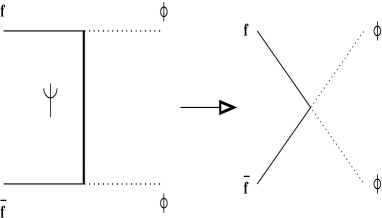
Figure 1: Branon $\phi$ creation from light fermions $f,\bar{f}$ due to super-heavy fermion $\Psi$ exchange.

However, it is quite plausible that the translation and $\tau$-symmetries are manifestly broken just because the five-dimensional world contains a classical background of gravitational and various matter fields with a net result similar to a crystal defect. In the present paper we have assumed the scalar nature of a five-dimensional space-time defect, which triggers the domain-wall formation through its coupling to the low-dimensional fermion operators. The two types of such defects have been investigated.

The first type is a non-topological one, the shape of which belongs to the Hilbert space of square integrable functions. In this case it happens that the only relevant dimensionless parameter $\xi$ governing the manifest symmetry breaking is given by a projection of the defect profile function on the Higgs boson wave function. The occurrence of such a defect supplies the branons with a small mass $\sim\xi\mu$ though its numerical value is rather model dependent. Meantime, the polarization of the domain wall background, i.e. its sign, is not correlated with the sign of a non-topological defect – for any sign, the local minimum of the low-energy effective action is attained.

The second type of defects is a topological one, with different non-vanishing asymptotics at the infinity. It makes much stronger the catalyzation of a domain wall, namely, the minimum and respectively the physical branon masses are reached only for coherent signs of the profiles of defect and domain-wall. In the latter case, again, the branons are supplied with a small mass.

Concerning the Higgs boson masses, their ratio to the fermion ($\sim$ top-quark) mass can be substantially reduced with an appropriate choice of a non-topological part of the defect $\sim\xi$. In particular, the Higgs masses may be well adjusted to a phenomenologically acceptable [52] value $\sim 135$ GeV for a reasonably small value of a defect $\xi\sim 0.4$.

In all scenarios the ratios of the induced coupling constants in the four-dimensional effective action for light particles are predicted unambiguously and in a model-independent way. Their absolute values are universally parameterized by the ratio of the symmetry breaking scale $M$ to the high-energy (compositeness) scale $\Lambda$ – a cutoff in the four-fermion interaction. This ratio $M/\Lambda<1$ can be thought of as an empirical input which must be established from the relevant experiments by measuring, for instance, the Yukawa coupling constant $g_{f}$ in the direct Higgs production via the fusion mechanism.

Figure 2: Missing energy in fermion annihilation due to branon emission.

However, the branon matter is much more elusive for experiments because it is not produced by fermions at the leading order in the Yukawa coupling and does not appear as a decay product of the Higgs bosons. Still the fermion annihilation (see, Fig. 2) may result in missing energy events due to radiative creation of branon pair mediated by Higgs bosons. The corresponding Feynman integral is well convergent and therefore, at very low momenta, the amplitude of this process can be estimated to be of order $g_{f}^{2}\cdot\lambda_{2}\cdot m^{2}_{f}/\mu^{2}$. We notice that if they are produced by very light fermions, e.g. $e^{+}e^{-}$, the very last ratio is negligibly small putting such signals into the experimental background. Nonetheless, for top-quarks (again in the fusion production) there might be a possibility to discover branon pair signals for sufficiently light branons. More qualitative estimates will be presented elsewhere. Anyhow, the sterile branons seem to be good candidates for saturation of the dark matter of our Universe – see Ref. [24] for a more detailed motivation.

Appendix A One-loop effective action

Let us consider the second order matrix-valued positive elliptic differential operator

$$D^{\dagger}D = -\partial_{\mu}\partial_{\mu}-\partial_{z}^{2}+{\cal M}^{2}(X)=-\partial^{2}+{\cal M}^{2}(X)\ ,$$

$${\cal M}^{2}(X) \equiv \Phi^{2}(X)+H^{2}(X)-\tau_{3}\not\!\partial\Phi(X)-\tau_{1}\not\!\partial H(X)\ ,$$ (130)

acting on a $n$-dimensional flat Euclidean space (eventually $n=5$). Our aim is to evaluate the matrix element of the distribution of the states operator: namely,

$$\langle X|\vartheta(Q^{2}-D^{\dagger}D)|Y\rangle=\int_{c-i\infty}^{c+i\infty}\frac{dt}{2\pi i}\ \frac{\exp\{tQ^{2}\}}{t}\,\langle X|\exp\{-tD^{\dagger}D\}|Y\rangle\ ,\quad c>0\ .$$ (131)

As a matter of fact, if the positive operator $D^{\dagger}D$ is also of the trace class, then the trace of $\vartheta(Q^{2}-D^{\dagger}D)$ does represent the number of the eigenstates of $D^{\dagger}D$ up to the momentum square $Q^{2}$. It is convenient to write the heat kernel in the form

$$\langle X|\exp\{-tD^{\dagger}D\}|Y\rangle\equiv(4\pi t)^{-n/2}\exp\left\{-\frac{(X-Y)^{2}}{4t}\right\}\Omega(t|X,Y)\ ,$$ (132)

where $\Omega(t|X,Y)$ is the so called transport function which fulfills

$$\left(\partial_{t}+\frac{X\cdot\partial}{t}+D^{\dagger}_{X}D_{X}\right)\Omega(t|X,Y)=0\ ,$$ (133)

$$\lim_{t\downarrow 0}\Omega(t|X,Y)={\bf 1}\ ,$$ (134)

in such a way that

$$\lim_{t\downarrow 0}\ \langle X|\exp\{-tD^{\dagger}D\}|Y\rangle={\bf 1}\delta^{(n)}(X-Y)\ .$$ (135)

If we insert Eq. (132) in Eq. (131) and change the integration variable we obtain

$$\langle X|\vartheta(Q^{2}-D^{\dagger}D)|Y\rangle = 2Q^{n}(4\pi)^{-1-n/2}\int_{c-i\infty}^{c+i\infty}dt\ t^{-1-n/2}$$ (136)

$$\times \exp\left\{t-\frac{Q^{2}(X-Y)^{2}}{4t}-\frac{i\pi}{2}\right\}\Omega\left(\frac{t}{Q^{2}}\left|X,Y\right.\right)\ .$$

Now, if we write

$$\Omega\left(\frac{t}{Q^{2}}\left|X,Y\right.\right)=\sum_{k=0}^{[n/2]}t^{k}a_{k}(X,Y)Q^{-2k}+{\cal R}_{[n/2]+1}\left(\frac{t}{Q^{2}}\left|X,Y\right.\right)\ ,$$ (137)

it turns out that, by insertion of Eq. (137) into the integral (136), the last term in the RHS of the above expression becomes sub-leading and negligible in the limit of very large $Q$. As a consequence, the leading asymptotic behavior of the matrix element (131) in the large $Q$ limit reads [53]

$$\langle X|\vartheta(Q^{2}-D^{\dagger}D)|Y\rangle \stackrel{{\scriptstyle Q\rightarrow\infty}}{{\sim}} (4\pi)^{-n/2}\sum_{k=0}^{[n/2]}a_{k}(X,Y)Q^{n-2k}$$ (138)

$$\times \int_{c-i\infty}^{c+i\infty}\frac{dt}{2\pi i}\ t^{k-1-n/2}\,\exp\left\{t-\frac{Q^{2}(X-Y)^{2}}{4t}\right\}$$

$$\stackrel{{\scriptstyle X\rightarrow Y}}{{\sim}} (4\pi)^{-n/2}\sum_{k=0}^{[n/2]}a_{k}(X,Y)\,\frac{Q^{n-2k}}{\Gamma(1-k+n/2)}\ .$$

In the diagonal limit $X=Y$, for $n=4,5$ the relevant coefficients of the heat kernel asymptotic expansion take the form [54]

$$a_{0}(X,X) \equiv {\bf 1}\ ;\qquad a_{1}(X,X)=-{\cal M}^{2}(X)\ ;$$

$$a_{2}(X,X) = \frac{1}{2}[{\cal M}^{2}(X)]^{2}-\frac{1}{6}\partial^{2}{\cal M}^{2}(X)\ ,$$ (139)

in such a way that we can finally write the dominant diagonal matrix element – leading eventually to the five-dimensional Euclidean effective Lagrange density – as

$$\langle X|\vartheta(Q^{2}-D^{\dagger}D)|X\rangle\stackrel{{\scriptstyle Q\rightarrow\infty}}{{\sim}}$$

$$\frac{Q^{5}}{60\pi^{3}}\left\{{\bf 1}-\frac{5}{2}Q^{-2}{\cal M}^{2}(X)+\frac{15}{8}Q^{-4}[{\cal M}^{2}(X)]^{2}-\frac{5}{8}Q^{-4}\partial^{2}{\cal M}^{2}(X)\right\}\ .$$ (140)

Appendix B Spectral resolution for Schrödinger operators

In this Appendix we calculate the spectra and eigenfunctions of the Schrödinger operators ${\rm M}_{J}^{11}$ and ${\rm M}_{J}^{22}$ arising in Eq.s (51) and (52) and presented in the factorized form in Eq.s (54) and (55). Let us choose the inverse mass units, $z=y/M$ and introduce the dimensionless operators

$${\rm M}_{J}^{11} \equiv M^{2}d^{+}_{\Phi}\equiv M^{2}q^{+}_{\Phi}\,q^{-}_{\Phi}\ ,$$ (141)

$${\rm M}_{J}^{22}-M^{2}+2\Delta_{2} \equiv M^{2}d^{+}_{H}\equiv M^{2}q^{+}_{H}\,q^{-}_{H}\ ,$$ (142)

$$q^{\pm}_{\Phi} = \mp\partial_{y}+2\mbox{\rm tanh}(y)\ ,$$ (143)

$$q^{\pm}_{H} = \mp\partial_{y}+\mbox{\rm tanh}(y)\ .$$ (144)

The two operators $d^{+}_{\Phi}$ and $d^{+}_{H}$ can be embedded into the supersymmetric ladder when one adds their supersymmetric partners

$$d^{-}_{\Phi}\equiv q^{-}_{\Phi}\,q^{+}_{\Phi}=d^{+}_{H}+3\ ,\qquad d^{-}_{H}\equiv q^{-}_{H}\,q^{+}_{H}=-\partial^{2}_{y}+1\ ,$$ (145)

the latter one describing a free particle propagation. The intertwining Darboux relations read

$$q^{\pm}_{\Phi}\,d^{\mp}_{\Phi}=d^{\pm}_{\Phi}\,q^{\pm}_{\Phi}\ ,$$

$$q^{\pm}_{H}\,d^{\mp}_{H}=d^{\pm}_{H}\,q^{\pm}_{H}\ ,$$

$$q^{-}_{H}\,q^{-}_{\Phi}\,d^{+}_{\Phi}=q^{-}_{H}(d^{+}_{H}+3)q^{-}_{\Phi}=(-\partial^{2}_{y}+4)q^{-}_{H}\,q^{-}_{\Phi}\ ,$$

$$d^{+}_{\Phi}\,q^{+}_{\Phi}\,q^{+}_{H}=q^{+}_{\Phi}\,q^{+}_{H}(-\partial^{2}_{y}+4)\ ,$$

$$q^{-}_{H}\,d^{+}_{H}=(-\partial^{2}_{y}+1)q^{-}_{H}\ ,$$

$$d^{+}_{H}\,q^{+}_{H}=q^{+}_{H}(-\partial^{2}_{y}+1)\ .$$ (146)

From these relations one concludes that the spectra of the operators $d^{+}_{\Phi}$ and $d^{+}_{H}$ are almost equivalent one to each other and, in turn, both equivalent to the free particle continuous spectrum – up to a shift of the origin. In other words, they consist of the continuous part and of the zero-modes of the intertwining operators $q^{-}_{H}q^{-}_{\Phi}$ and $q^{-}_{H}$ respectively. Owing to Eq.s (146) their eigenvalues and normalized improper eigenfunctions are related as follows: namely,

$$\psi_{\Phi}(ky)\doteq\frac{q^{+}_{\Phi}\,\psi_{H}(ky)}{\sqrt{k^{2}+4}}\doteq\frac{q^{+}_{\Phi}q^{+}_{H}\,\psi_{0}(ky)}{\sqrt{(k^{2}+1)(k^{2}+4)}}\ ,\qquad E^{c}_{\Phi}(k)=k^{2}+4\ ,$$

$$\psi_{H}(ky)\doteq\frac{q^{+}_{H}\,\psi_{0}(ky)}{\sqrt{k^{2}+1}}\ ,\qquad\quad E^{c}_{H}(k)=k^{2}+1\ ,$$

$$\psi_{0}(ky)=\frac{1}{\sqrt{2\pi}}\exp(iky)\ ,\qquad\qquad k\in{\bf R}\ .$$ (147)

The imprecise equality $\doteq$ signifies a possible discrepancy due to the existence of zero-modes. In particular, for the operator $d^{+}_{H}$ the continuum starts from $E^{c}_{H}(0)=1$ and the only zero-mode $h_{0}(y)=\left(1/\sqrt{2}\right)\,\mbox{\rm sech}(y)$ just coincides with the zero-mode of $q^{-}_{H}$. Concerning the operator $d^{+}_{\Phi}$, one can easily verify that the continuum starts from $E^{c}_{\Phi}(0)=4$, whereas the zero-mode $\phi_{0}(y)=\left(\sqrt{3}/2\right)\,\mbox{\rm sech}^{2}(y)$ coincides with the zero-mode of $q^{-}_{\Phi}$. Furthermore, the second parity-odd proper eigenstate

$$\phi_{1}(y)=\left(1/\sqrt{3}\right)\,q^{+}_{\Phi}h_{0}(y)=\sqrt{3/2}\,{\mbox{\rm tanh}(y)}\,{\mbox{\rm sech}(y)}\ ,$$ (148)

does coincide with the zero-mode of $q^{-}_{H}\,q^{-}_{\Phi}$ and corresponds to the first non-vanishing, discrete eigenvalue $E^{+}_{\Phi}=3$.

Appendix C Perturbation theory for the first excited state

In this Appendix we develop the perturbation theory for the first excited eigenstate and the corresponding eigenvalue of the operator ${\bf M}_{K}$ defined in Eq. (73). As in the Appendix B the inverse mass units $z=y/\beta$ are chosen, so that the dimensionless operator $\Xi\equiv{\bf M}_{K}/\beta^{2}$ has the following components in terms of the operators in Eq.s  (141)-(144): namely,

$$\Xi=\left\lgroup\begin{array}[]{cc}d^{+}_{\Phi}&0\\ 0&d^{+}_{H}\end{array}\right\rgroup\ +4\epsilon\,{\mbox{\rm sech}^{2}(y)}\left\lgroup\begin{array}[]{cc}\epsilon\,{\mbox{\rm sinh}^{2}(y)}&\sqrt{1+\epsilon^{2}}\ {\mbox{\rm sinh}(y)}\\ \sqrt{1+\epsilon^{2}}\ {\mbox{\rm sinh}(y)}&\epsilon\end{array}\right\rgroup\ .$$ (153)

The second, perturbation term contains the elements of different order in $\epsilon$. This is the ultimate reason why, in order to compute the corrections to the eigenvalues, we have to take into account not only the eigenfunction of zeroth-order, but also the first-order correction turns out to be necessary. Thus we use the eigenfunction $h_{K}(y)=[h^{-}_{K}(y),h^{+}_{K}(y)]$ from Eq. (86), taking into account that, to the lowest order, the parity-odd function $h^{-}_{K}(y)$ is of order $\epsilon$ and the parity-even one is $h^{+}_{K}(y)\simeq h_{0}(y)=\left(1/\sqrt{2}\right)\,\mbox{\rm sech}(y)$. To the first order in $\epsilon$, the function $h^{+}_{K}(y)$ is derived from the following equation

$$d^{+}_{\Phi}\,h^{-}_{K}(y) = -4\epsilon\,{\mbox{\rm tanh}(y)}\,{\mbox{\rm sech}(y)}\,h_{0}(y)=-\frac{4\epsilon}{\sqrt{2}}\,{\mbox{\rm tanh}(y)}\,{\mbox{\rm sech}^{2}(y)}$$ (154)

$$= -\ \frac{\epsilon}{\sqrt{2}}\,q^{+}_{\Phi}\,{\mbox{\rm sech}^{2}(y)}\ ,$$

which follows from the basic definition $\Xi h_{K}=E_{h}h_{K}$ and the estimation of $E_{h}\sim\epsilon^{2}$. Since there are no normalizable zero-modes for the operator $q^{+}_{\Phi}$ one concludes that

$$q^{-}_{\Phi}\,h^{-}_{K}(y)=-\frac{\epsilon}{\sqrt{2}}\,{\mbox{\rm sech}^{2}(y)}\ ,$$ (155)

which represents a first-order differential equation with the normalizable solution

$$h^{-}_{K}(y)=-\frac{\epsilon}{\sqrt{2}}\,y\,{\mbox{\rm sech}^{2}(y)}\ .$$ (156)

Now, the eigenvalue $E_{h}$ can be obtained from its integral representation $E_{h}=\langle h_{K}\left|\,\Xi\,\right|h_{K}\rangle$ in terms of the normalizable function $\langle h_{K}|h_{K}\rangle=1$. To the first order in $\epsilon$ it reads eventually

$$E_{h}=4\int^{+\infty}_{-\infty}dy\ h_{0}(y)\left\{\epsilon^{2}{\mbox{\rm sech}^{2}(y)}\,h_{0}(y)+\epsilon\,{\mbox{\rm tanh}(y)}\,{\mbox{\rm sech}(y)}\,h^{-}_{K}(y)\right\}=2\epsilon^{2}\ .$$ (157)

Appendix D Perturbation theory in the presence of defects

The inclusion of a small regular defect is described by the scalar functions ${\rm f}_{\Phi}(z),{\rm f}_{H}(z)$ and leads to the change of the mass matrix ${\bf M}_{K}$ presented in Eq. (108) for the ansatz $(A)$ and in Eq. (127) for the ansatz $(B)$. If we introduce the dimensionless operators $\Xi_{j}\,,\quad j=A,B\,$, then according to the notations of Eq. (153) we obtain

$$\Xi_{j}=\Xi_{K}+{\bf\Delta}_{j}\ ,$$ (158)

$$\Delta_{A}^{11}\approx\epsilon^{2}\,{\mbox{\rm sech}^{2}(y)}\,[\,4\xi+2\xi^{2}-12y\ {\mbox{\rm tanh}(y)}\,]\ ,$$

$$\Delta_{A}^{12}=\Delta_{A}^{21}\approx 4\epsilon\,\xi\ {\mbox{\rm sech}^{2}(y)}\,{\mbox{\rm sinh}(y)}\ ,$$ (159)

$$\Delta_{A}^{22}\approx\epsilon^{2}\,{\mbox{\rm sech}^{2}(y)}\,[\,12\xi+6\xi^{2}-4y\ {\mbox{\rm tanh}(y)}\,]\ ,$$

$$\Delta_{B}^{11}\approx\epsilon^{2}\,{\mbox{\rm sech}^{2}(y)}\left[\,4\xi\ +2\xi^{2}+3(\gamma-4\xi\ -2\xi^{2})\,y\,{\mbox{\rm tanh}(y)}+3\gamma{\mbox{\rm sinh}^{2}(y)}\,\right]\ ,$$

$$\Delta_{B}^{12}\approx\Delta_{B}^{21}=4\xi\epsilon\,{\mbox{\rm sech}^{2}(y)}{\mbox{\rm sinh}(y)}\ ,$$ (160)

$$\Delta_{B}^{22}\approx\epsilon^{2}\,{\mbox{\rm sech}^{2}(y)}\left[\,12\xi\ +6\xi^{2}+(\gamma-4\xi\ -2\xi^{2})\,y\,{\mbox{\rm tanh}(y)}+\gamma{\mbox{\rm sinh}^{2}(y)}\,\right]\ ,$$

One can see that again the perturbation matrices contain elements of different order in $\epsilon$ and therefore the calculation of energy levels needs first to derive the perturbed eigenfunctions to a relevant order in $\epsilon$ as it has been done in the Appendix C.

To the relevant order in $\epsilon$, the eigenvalue equations for the scalar wave function components $s_{A}^{+}(y),s_{A}^{-}(y)$ follow from the matrix elements of the operator in Eq. (158),

$$(d^{+}_{\Phi}-E_{s})\ s_{j}^{+}(y)+\Bigl{[}\,4\epsilon^{2}\,{\mbox{\rm tanh}^{2}(y)}+\Delta_{j}^{11}\,\Bigr{]}\ s_{j}^{+}(y)$$

$$+4\epsilon\ (1+\xi)\ {\mbox{\rm sech}^{2}(y)}\ {\mbox{\rm sinh}(y)}\ s_{j}^{-}(y)=0\ ,$$

$$(d^{+}_{H}-E_{s})\ s_{j}^{-}(y)+\Bigl{[}\,4\epsilon^{2}\,{\mbox{\rm sech}^{2}(y)}\,+\Delta_{j}^{22}\,\Bigr{]}\ s_{j}^{-}(y)$$

$$+4\epsilon\ (1+\xi)\ {\mbox{\rm sech}^{2}(y)}\ {\mbox{\rm sinh}(y)}\ s_{j}^{+}(y)=0\ .$$ (161)

These equations have terms of different order in $\epsilon$ in two sectors of solutions.

Actually, for even-odd solutions with $s_{j}^{\pm}(y)=\phi^{\pm}_{j}(y)$, the upper even component $\phi_{j}^{+}=\phi^{+(0)}+\epsilon^{2}\phi_{j}^{+(1)}+{\cal O}(\epsilon^{4})$ contains the zero mode (84) of the operator $d^{+}_{\Phi}$ as a leading term. Meanwhile, the lower odd component $\phi_{j}^{-}$ has an order of $\epsilon$ and coincides with the unperturbed one – see Eq. (84) in its functional form. Indeed, as one expects that the lightest eigenvalues are of the order $E_{s}\sim\epsilon^{2}$, then the dominating part of the second Eq. (161) reads,

$$d^{+}_{H}\,\phi_{j}^{-(0)}+4\epsilon\ (1+\xi)\ {\mbox{\rm tanh}(y)}\,{\mbox{\rm sech}(y)}\,\phi^{+(0)}=0.$$ (162)

Comparing this equation with the unperturbed one, corresponding to $\xi=0$, from Eq. (84) one immediately finds that

$$\phi_{j}^{-(0)}(y)=-\sqrt{\frac{3\beta}{4}}\,\epsilon\ (1+\xi)\ {\mbox{\rm sinh}(y)}\,{\mbox{\rm sech}^{2}(y)}\equiv\phi^{-(0)}(y)\ .$$ (163)

On the other hand, as $d^{+}_{\Phi}\,\phi^{+(0)}=0$ the first Eq. (161) determines the next-to-leading contribution $\phi_{j}^{+(1)}$ into the even part of the wave function. Now this equation allows us to obtain both the approximate eigenvalue and the correction term $\phi_{j}^{+(1)}$. After projection onto the zero-mode $\phi_{j}^{+(0)}$ of the operator $d^{+}_{\Phi}$, one gets rid of the unknown function $\phi_{j}^{+(1)}$ and calculates eventually the branon mass: namely,

$$\left(m^{j}_{\phi}\right)^{2} = \beta^{2}E_{\phi}=\beta^{2}\int^{+\infty}_{-\infty}dy\ \left\{\Bigl{[}\,4\epsilon^{2}\,{\mbox{\rm tanh}^{2}(y)}+\Delta_{j}^{11}\,\Bigr{]}\left[\,\phi^{+(0)}(y)\,\right]^{2}\right.$$ (164)

$$\left.+4\epsilon\,(1+\xi)\ {\mbox{\rm sech}^{2}(y)}\ {\mbox{\rm sinh}(y)}\,\phi^{-(0)}(y)\,\phi^{+(0)}(y)\right\}\ .$$

In the sector of odd-even solutions $s_{j}^{\pm}(y)=h^{\mp}_{j}(y)$ the lightest-state wave function has the opposite order in $\epsilon$, i.e.,

$$h^{-(0)}_{j}(y)\sim\epsilon,\ \ h^{+}_{j}(y)=h^{+(0)}+\epsilon^{2}h_{j}^{+(1)}+{\cal O}(\epsilon^{4})\ .$$

Thus the role of two Eq.s (161) is merely interchanged. In particular, it can be easily derived that

$$h^{-(0)}_{j}(y)=-\ \epsilon\,(1+\xi)\ y\,{\mbox{\rm sech}^{2}(y)}/\sqrt{2}\equiv h^{-(0)}(y)\ ,$$

$$h^{+(0)}(y)=\ \mbox{\rm sech}(y)/\sqrt{2}\ ,$$ (165)

to be compared with Eq. (86). Respectively, when we project onto the zero-mode $h^{+(0)}_{j}(y)$ of the operator $d^{+}_{H}$, the second equation helps us to obtain the Higgs boson mass,

$$\left(m^{j}_{h}\right)^{2} = \beta^{2}E_{h}=\beta^{2}\int^{+\infty}_{-\infty}dy\ \left\{\Bigl{[}\,4\epsilon^{2}\,{\mbox{\rm sech}^{2}(y)}\,+\Delta_{j}^{22}\,\Bigr{]}\left[\,h^{+(0)}(y)\,\right]^{2}\right.$$ (166)

$$\left.+4\epsilon\,(1+\xi)\ {\mbox{\rm sech}^{2}(y)}\,{\mbox{\rm sinh}(y)}\,h^{-(0)}(y)\,h^{+(0)}(y)\right\}\ .$$