DESY 03–064

DFF 403/05/03

LPTHE–03–15

hep-ph/0305254

Extending QCD perturbation theory to higher energies

M. Ciafaloni^(a), D. Colferai^(a), G. P. Salam^(b) and A. M. Staśto^(c)
(a) Dipartimento di Fisica, Universitá di Firenze, 50019 Sesto Fiorentino (FI), Italy;

INFN Sezione di Firenze, 50019 Sesto Fiorentino (FI), Italy

^(b) LPTHE, Universités Paris VI and VII, CNRS UMR 7589, Paris 75005, France

^(c) Theory Division, DESY, D22603 Hamburg, Germany;

H. Niewodniczański Institute of Nuclear Physics, Kraków, Poland

On the basis of the results of a new renormalisation group improved small-$x$ resummation scheme, we argue that the range of validity of perturbative calculations is considerably extended in rapidity with respect to leading log expectations. We thus provide predictions for the energy dependence of the gluon Green function in its perturbative domain and for the resummed splitting function. As in previous analyses, high-energy exponents are reduced to phenomenologically acceptable values. Additionally, interesting preasymptotic effects are observed. In particular, the splitting function shows a shallow dip in the moderate small-$x$ region, followed by the expected power increase.

PACS 12.38.Cy, 13.85.-t

1 Introduction

The prediction of high-energy hard cross sections in QCD perturbation theory has been a puzzling problem in recent years for a number of reasons: the existence of large perturbative leading $\log s$ (LL) contributions [1] that seem incompatible with a range of experimental data; the discovery of even larger subleading contributions (NLL) of opposite sign [2, 3]; and the increasing importance of low-$k_{t}$ partons at high energies leading asymptotically to a strong-coupling Pomeron regime which can at best be modelled but not really predicted [4, 5, 6, 7].

In order to tame the problem of large logarithms with alternating sign several resummation procedures have been proposed [8, 9, 10, 11, 12, 13, 14, 15]. The renormalisation group improved (RGI) approach [8, 9, 10] offers a general understanding of the large subleading $\log s$ terms as due to leading $\log Q^{2}$ collinear contributions which can be extracted on the basis of the perturbative anomalous dimensions. As a result, resummed high-energy exponents have been calculated in a stable way. In a forthcoming paper [16] this resummation approach is extended to the gluon Green’s function and splitting function so as to provide a fairly complete account of their energy dependence and of its perturbative (PT) versus non-perturbative (NP) aspects. The purpose of the present paper is to summarise the main results of Ref. [16] and to argue, on this basis, that the RGI approach tames – to a large extent – the problem of the strong-coupling region as well. This is because the resummation of the (alternating sign) large logarithms leads to smaller high-energy exponents (and diffusion coefficients) and to a considerable suppression of the non-perturbative Pomeron itself in the Green function. Furthermore, we find that strong-coupling contributions factorise, as expected, in the collinear limit, and we are able to provide the resummed perturbative splitting function in $x$-space.

The basic problem that we consider is the calculation of the (azimuthally averaged) gluon Green function $G(Y;k,k_{0})$ as a function of the magnitudes of the external gluon transverse momenta $k\equiv|{\boldsymbol{k}}|,\;k_{0}\equiv|{\boldsymbol{k}}_{0}|$ and of the rapidity $Y\equiv\log\frac{s}{kk_{0}}$. This is not yet a hard cross section, because we need to incorporate [16] the impact factors of the probes [17, 18, 19]. Nevertheless, the Green function exhibits most of the physical features of the hard process, if we think of $k^{2},\;k_{0}^{2}$ as external (hard) scales. The limits $k^{2}\gg k_{0}^{2}$ ($k_{0}^{2}\gg k^{2}$) correspond conventionally to the ordered (anti-ordered) collinear limit. By definition, in the $\omega$-space conjugate to $Y$ (so that $\hat{\omega}=\partial_{Y}$) we set

$${\cal G}_{\omega}({\boldsymbol{k}},{\boldsymbol{k}}_{0}) \equiv[\omega-{\cal K}_{\omega}]^{-1}({\boldsymbol{k}},{\boldsymbol{k}}_{0})\,,$$ (1)

$$\omega{\cal G}_{\omega}({\boldsymbol{k}},{\boldsymbol{k}}_{0}) =\delta^{2}({\boldsymbol{k}}-{\boldsymbol{k}}_{0})+\int d^{2}{\boldsymbol{k}}^{\prime}\;{\cal K}_{\omega}({\boldsymbol{k}},{\boldsymbol{k}}^{\prime}){\cal G}_{\omega}({\boldsymbol{k}}^{\prime},{\boldsymbol{k}}_{0})\;,$$ (2)

where ${\cal K}_{\omega}({\boldsymbol{k}},{\boldsymbol{k}}^{\prime})$ is a kernel to be defined, whose $\omega=0$ limit is related to the BFKL $Y$-evolution kernel, known at LL and NLL levels [2, 3].

The RGI approach is based on the simple observation that, in BFKL iteration, all possible orderings of transverse momenta are to be included, the ordered (anti-ordered) sequence $k\gg k_{1}\cdots\gg k_{n}\cdots\gg k_{0}$ ($k\ll k_{1}\cdots\ll k_{n}\cdots\ll k_{0}$) showing scaling violations with Bjorken variable $k^{2}/s$ ($k_{0}^{2}/s$). Therefore, if only leading $\log k^{2}$ contributions were to be considered, the kernel ${\cal K}_{\omega}$ acting on $\frac{1}{k^{2}}\left(\frac{k^{2}}{k_{0}^{2}}\right)^{\gamma}$ would be approximately represented by the following eigenvalue function (in the frozen coupling limit)

$$\frac{1}{\omega}{\cal K}_{\omega}\rightarrow\bar{\alpha}_{s}\left(\frac{1}{\gamma+{\textstyle\frac{\omega}{2}}}+\frac{1}{1+{\textstyle\frac{\omega}{2}}-\gamma}\right)\left(\frac{1}{\omega}+A_{1}(\omega)\right)+\cdots\;,\qquad\bar{\alpha}_{s}\equiv\alpha_{s}\frac{N_{c}}{\pi}\;,$$ (3)

where $\gamma^{(1)}_{gg}=\bar{\alpha}_{s}\left(\frac{1}{\omega}+A_{1}(\omega)\right)$ is the one-loop gluon-gluon anomalous dimension and we have introduced the variable $\gamma$ conjugate to $\log k^{2}$. Note, in fact, that Eq. (3) reduces to the normal DGLAP evolution [20] in $\log k^{2}$ ($\log k_{0}^{2}$) in the two orderings mentioned before, because $\gamma+{\textstyle\frac{\omega}{2}}$ ($1+{\textstyle\frac{\omega}{2}}-\gamma$) is represented by $\partial_{\log k^{2}}$ ($\partial_{\log k_{0}^{2}}$) at fixed values of $x=k^{2}/s$ ($x_{0}=k_{0}^{2}/s$) in the ordered (anti-ordered) momentum region. Note also the $\omega$-dependent shift [8, 9, 10] of the $\gamma$-singularities occurring in Eq. (3), which is required by the change of scale ($k_{0}^{2}$ versus $k^{2}$) needed to interchange the orderings, i.e., $x_{0}$ versus $x$.

We thus understand that the $\omega$-dependence of ${\cal K}_{\omega}$ is essential for the resummation of the collinear terms and can be used to incorporate the exact LL collinear behaviour, while on the other hand, the $\omega\to 0$ behaviour of ${\cal K}_{\omega}$ is fixed by the BFKL limit up to $\mathcal{O}\left(\omega\right)$ terms, so as to incorporate exact LL and NLL kernels. Such requirements fix the kernel up to contributions that are NNL in $\ln x$ and NL in $\ln Q^{2}$. The form proposed in [16] (there called $\mathrm{NLL_{B}}$) is given by

$${\cal K}_{\omega}=\left(\bar{\alpha}_{s}(x_{\mu}^{2}q^{2})+b\bar{\alpha}_{s}^{2}\ln x_{\mu}^{2}\right)K^{\omega}_{0}+\omega\left(\bar{\alpha}_{s}(x_{\mu}^{2}k_{>}^{2})+b\bar{\alpha}_{s}^{2}\ln x_{\mu}^{2}\right)K^{\omega}_{c}+\bar{\alpha}_{s}^{2}(x_{\mu}^{2}k_{>}^{2})\tilde{K}^{\omega}_{1}\,,$$ (4)

where $q\equiv|{\boldsymbol{k}}-{\boldsymbol{k}}^{\prime}|$, $k_{>}\equiv\max(k,k^{\prime})$, $k_{<}\equiv\min(k,k^{\prime})$, $x_{\mu}$ has been introduced to test renormalisation-scale dependence, and the scale-invariant kernels in the RHS have the eigenvalue functions

$$\chi_{0}^{\omega}(\gamma) =2\psi(1)-\psi(\gamma+{\textstyle\frac{\omega}{2}})-\psi(1-\gamma+{\textstyle\frac{\omega}{2}})\,,$$ (5a)

$$\chi_{{\mathrm{c}}}^{\omega}(\gamma) =\frac{A_{1}(\omega)}{\gamma+{\textstyle\frac{\omega}{2}}}+\frac{A_{1}(\omega)}{1-\gamma+{\textstyle\frac{\omega}{2}}}\,,$$ (5b)

$$\tilde{\chi}_{1}^{\omega}(\gamma) =\chi_{1}(\gamma)+\frac{1}{2}\chi_{0}(\gamma)\frac{\pi^{2}}{\sin^{2}(\pi\gamma)}-\chi_{0}(\gamma)\frac{A_{1}(0)}{\gamma(1-\gamma)}+\frac{b}{2}\left[\chi^{\prime}_{0}(\gamma)+\chi_{0}^{2}(\gamma)\right]$$

$$\quad-\left(\frac{1}{\gamma}+\frac{1}{1-\gamma}\right)C(0)+\left(\frac{1}{\gamma+{\textstyle\frac{\omega}{2}}}+\frac{1}{1+{\textstyle\frac{\omega}{2}}-\gamma}\right)C(\omega)[1+\omega A_{1}(\omega)]\,,$$ (5c)

with $b=\frac{11}{12}-\frac{n_{f}}{6N_{c}}$, $C(\omega)=\frac{\psi(1+\omega)-\psi(1)}{\omega}-\frac{A_{1}(\omega)}{\omega+1}$ and

$$\chi_{0}(\gamma) =\chi_{0}^{\omega=0}(\gamma)=2\psi(1)-\psi(\gamma)-\psi(1-\gamma)\,,$$ (6)

$$\chi_{1}(\gamma) =-\frac{b}{2}[\chi^{2}_{0}(\gamma)+\chi^{\prime}_{0}(\gamma)]-\frac{1}{4}\chi_{0}^{\prime\prime}(\gamma)-\frac{1}{4}\left(\frac{\pi}{\sin\pi\gamma}\right)^{2}\frac{\cos\pi\gamma}{3(1-2\gamma)}\left(11+\frac{\gamma(1-\gamma)}{(1+2\gamma)(3-2\gamma)}\right)$$

$$\quad+\left(\frac{67}{36}-\frac{\pi^{2}}{12}\right)\chi_{0}(\gamma)+\frac{3}{2}\zeta(3)+\frac{\pi^{3}}{4\sin\pi\gamma}$$

$$\quad-\sum_{n=0}^{\infty}(-1)^{n}\left[\frac{\psi(n+1+\gamma)-\psi(1)}{(n+\gamma)^{2}}+\frac{\psi(n+2-\gamma)-\psi(1)}{(n+1-\gamma)^{2}}\right]\;.$$ (7)

All $n_{f}$ dependence other than that in the running coupling terms (that is in $b$) has been neglected. A correct treatment of all $n_{f}$-dependent RG contributions would make the formalism technically more complex (e.g. requiring a two-channel approach) and given the observed small effect of the $n_{f}$ contributions, we feel such an effort to be currently uncalled for.

Note that, because of the explicit form of $\chi_{0}^{\omega}$, the kernel (4) reproduces the pole behaviour (3) to first order in $\alpha_{s}$. Note also that the last line in Eq. (5c), which vanishes in the $\omega=0$ limit, has been added in order to shift the remaining $C(0)/\gamma$ and $C(0)/(1-\gamma)$ poles in $\chi_{1}$. There is some freedom in the choice of the $\omega$-dependence of the coefficient of the shifted poles, and we take here a minimal prescription, one that gives an indentically zero two-loop contribution to the anomalous dimension (we refer to this prescription as $\mathrm{NLL_{B}}$). This also guarantees that the momentum sum-rule is satisfied at two-loop level. Note finally that the resummed kernel proposed here differs from that of [10] because the collinear terms are added in the $\omega$-dependent form, the difference being at NNLL level. The reason for such a change is that we have at most simple collinear poles, as in Eq. (3), and not double poles. This avoids the need for the $\omega$ expansion, thus providing a kernel more suitable for numerical iteration in ($x,k$)-space.

The integral equation to be solved by the definition (2) is thus a running coupling equation with non linear dependence on $\alpha_{s}$ at appropriate scales, and it has a somewhat involved $\omega$-dependence in the improved kernels (5). Its solution has been found in [16] by numerical matrix evolution methods in $k$- and $x$- space [21], where the typical $\omega$-shifted form in the example (3) corresponds to the so-called consistency constraint [22, 23, 24]. Furthermore, introducing the integrated gluon density

$$xg(x,Q^{2})\equiv\int^{Q^{2}}d^{2\!}{\boldsymbol{k}}\;G^{(s_{0}=k^{2})}(\log 1/x;|{\boldsymbol{k}}|,k_{0})\;,\qquad{\cal G}_{\omega}^{(s_{0}=k^{2})}\equiv\left(\frac{k}{k_{0}}\right)^{\omega}{\cal G}_{\omega}\;,$$ (8)

the resummed splitting function $P_{\mathrm{eff}}(z,Q^{2})$ is defined by the evolution equation

$$\frac{\partial g(x,Q^{2})}{\partial\log Q^{2}}=\int\frac{dz}{z}\;P_{\mathrm{eff}}(z,Q^{2})\;g\left(\frac{x}{z},Q^{2}\right)\,,$$ (9)

and has been extracted [16] by a numerical deconvolution method [25]. We note immediately that $P_{\mathrm{eff}}$ turns out to be independent of $k_{0}$ for $Q^{2}\gg k_{0}^{2}$, yielding an important check of RG factorisation in our approach.

2 Gluon Green’s function

Results for $G(Y;k,k)$ are shown in Fig. 1. In addition to the solution based on our RGI approach ($\mathrm{NLL_{B}}$) the figure also has ‘reference’ results for LL evolution with kernel $\bar{\alpha}_{s}(x_{\mu}^{2}q^{2})K^{0}_{0}$. We use a one-loop running coupling with $n_{f}=4$, which is regularised either by setting it to zero below a scale ${\bar{k}}$ (‘cutoff’) or by freezing it below that scale ($\alpha_{s}(q^{2}<{\bar{k}}^{2})=\alpha_{s}({\bar{k}}^{2})$). We believe the cutoff regularisation to be more physical since it prevents diffusion to arbitrarily small scales and is thus more consistent with confinement — accordingly we show three cutoff regularisations and only one frozen regularisation. The ${\bar{k}}=0.74\,\,\mathrm{GeV}$ cutoff solution is presented together with an uncertainty band associated with the variation of $x^{2}_{\mu}$ between $\frac{1}{2}$ and $2$.

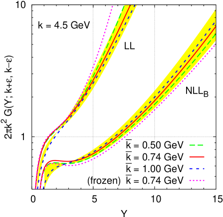
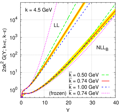
Figure 1: Green’s function calculated with four different infrared regularisations of the coupling, shown for LL and RGI NLL (‘NLL${}_{\mathrm{B}}\!$’) evolution. The bands indicate the sensitivity of the ${\bar{k}}=0.74\,\,\mathrm{GeV}$ results to a variation of $x^{2}_{\mu}$ in the range $\frac{1}{2}$ to $2$. The left and right hand plots differ only in their scales.

Solutions of (2) with an IR-regularised coupling generally have two domains [4, 5, 6, 26], separated by a critical rapidity $Y_{c}(k^{2})$. For the intermediate high-energy region $1\ll Y\lesssim Y_{c}(k^{2})$, one expects the perturbative ‘hard Pomeron’ behaviour with exponent $\omega_{s}$,

$$k^{2}G(Y;k,k)\sim\frac{1}{\sqrt{Y}}\exp\big{[}\omega_{s}(\alpha_{s}(k^{2}))Y+\Delta(\alpha_{s},Y)\big{]}\;,$$ (10)

and diffusion corrections [27, 28, 29, 30] parametrised by $\Delta(\alpha_{s},Y)$. Beyond $Y_{c}$, a regularisation-dependent non-perturbative ‘Pomeron’ regime takes over

$$k^{2}G(Y;k,k)\sim\left(\frac{{\bar{k}}^{2}}{k^{2}}\right)^{\xi}e^{\omega_{\mathbb{P}}Y}\,,\qquad\begin{array}[]{rl}\mathrm{LL}\;\,\,:&\xi=1\\ \mathrm{NLL}_{B}:&\xi=1+\omega_{\mathbb{P}}\end{array}$$ (11)

where the factor $\xi$ differs from $1$ only for kernels involving the consistency constraint. The non-perturbative exponent $\omega_{\mathbb{P}}$ satisfies [10] $\omega_{\mathbb{P}}\sim\omega_{s}(\alpha_{s}({\bar{k}}^{2}))$ and hence is formally larger than $\omega_{s}(\alpha_{s}(k^{2}))$.

The value of $Y_{c}$ depends strongly on $k$. In the tunnelling approximation, it can be roughly estimated by equating eqs. (10) and (11) to yield [31, 26], for any given regularisation procedure,

$$Y_{c}(k^{2})\simeq\frac{\xi\log(k^{2}/{\bar{k}}^{2})}{\omega_{\mathbb{P}}-\omega_{s}(\alpha_{s}(k^{2}))}\;,$$ (12)

(again with $1+\omega_{\mathbb{P}}\to 1$ for LL), showing an approximately linear increase of $Y_{c}$ with $\log k^{2}$.

Within this logic, several aspects of Fig. 1 are worth commenting. The most striking feature of the LL evolution is its strong dependence on the non-perturbative regularisation, even for rapidities as low as $5$. The exact value of $Y_{c}$ depends on the regularisation being used, ranging between $5$ and $10$. In contrast, $\mathrm{NLL_{B}}$ evolution remains under perturbative control up to much larger rapidities and the NP pomeron behaviour takes over only for $Y\gtrsim 25$, where the three cutoff solutions start to diverge. Regularisation dependence is also present at lower rapidities. This seems to be due to power corrections to (10), associated with the use of a coupling $\alpha_{s}(q^{2})$ [16]. The non-perturbative regime of the IR frozen coupling solution is reached only later ($Y\gtrsim 30$), at the point where it starts to grow more rapidly than the cutoff solutions. A final point to note is renormalisation scale uncertainties of our resummed results are sizeable – of the order of several tens of percent for $Y>4$ – but seem anyhow quite modest compared to the order(s) of magnitude difference with LL.

The fact that $Y_{c}$ is considerably larger for $\mathrm{NLL_{B}}$ evolution is natural — it is an expected consequence (see Eq.(12)) of the fact that subleading corrections lower both the PT and NP exponents. What is quite non-trivial however is that at their respective $Y_{c}$’s the $\mathrm{NLL_{B}}$ Green’s function is an order of magnitude larger than the LL one: the subleading corrections increase the overall amount of BFKL growth remaining within perturbative control. This is due to a number of factors, among them a strong reduction of the diffusion coefficient (see below). We note that the increase in the amount of perturbatively calculable growth is of particular interest for the theoretical question (see e.g. [27]) of whether it is possible to perturbatively generate a high-density gluonic system.

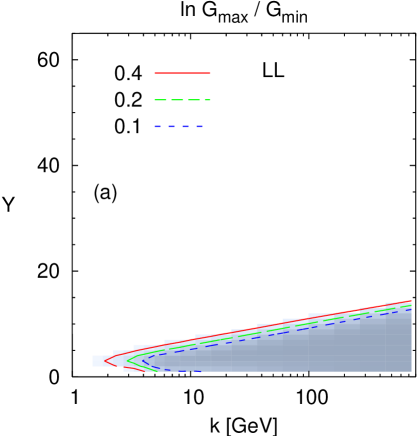
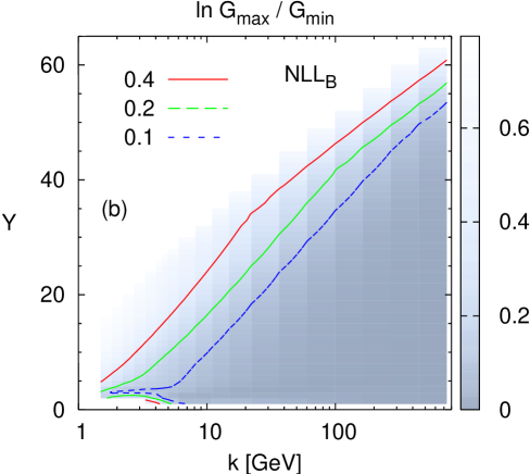
Figure 2: Contour plots showing the sensitivity of $G(Y,k+\epsilon,k-\epsilon)$ to one’s choice of non-perturbative regularisation, as obtained by examining the logarithm of the ratio of the regularisations giving the largest and smallest result for $G$. Darker shades indicate insensitivity to the NP regularisation, and contours have been drawn where the logarithm of the ratio is equal to $0.1$, $0.2$ and $0.4$. Plot (a) shows the result for LL evolution, while (b) shows RGI NLL evolution ($\mathrm{NLL_{B}}$). The regularisations considered are those of Fig. 1.

In Fig. 1 we have considered only a single value of $k$. The question of NP contributions is summarised more generally in Fig. 2, which shows contour plots of the logarithmic spread of our four regularisations. Darker regions are less IR sensitive, and contours for particular values of the spread have been added to guide the eye. Here too one clearly sees the much larger region (including most of the phenomenologically interesting domain) that is accessible perturbatively after accounting for subleading corrections.

So let us now therefore return to Fig. 1 and examine the characteristics of the $\mathrm{NLL_{B}}$ Green’s function in the perturbatively accessible domain, which should be describable by an equation of the form (10). The first feature to note is that the growth starts only from $Y\simeq 4$. This suggests that at today’s collider energies (implying $Y\lesssim 6$ [32, 33]), it will at best be possible to see only the start of any growth. This preasymptotic feature is partly due to the slow opening of small-$x$ phase space [34] implicit in our $\omega$–shifting procedure.

Once the growth sets in, the issue is to establish the value of $\omega_{s}$ appearing in (10). This is a conceptually complex question because in contrast to the fixed-coupling case, $\omega_{s}$ no longer corresponds to a Regge singularity. There are running-coupling diffusion corrections $\Delta(\alpha_{s},Y)$ [27, 28, 29, 30], whose leading contribution, $\sim Y^{3}$, for our model is [16]

$$\Delta(\alpha_{s},Y)\simeq\frac{Y^{3}}{24}\left[\frac{\partial}{\partial\log k^{2}}\omega_{s}(\alpha_{s}(k^{2}))\right]^{2}\chi_{\mathrm{eff}}^{\prime\prime}({\textstyle\frac{1}{2}})\,.$$ (13)

In addition, $\Delta(\alpha_{s},Y)$ contains terms with weaker $Y$ dependences, including $Y^{2}$ and $Y$. Such terms can be disentangled by the method of the $b$-expansion [35].

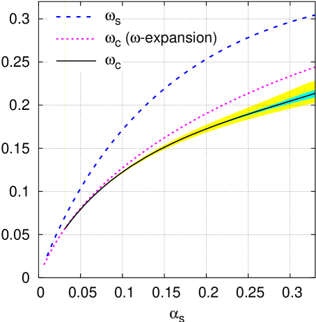
Figure 3: The small-$x$ exponents: the Green’s function effective exponent $\omega_{s}$ is shown to first order in the $b$-expansion; the splitting function exponent $\omega_{c}$ is shown together with NP and renormalisation scale uncertainty bands, defined in figure 4. Also shown, for reference, is the result for $\omega_{c}$ using the method of [10], for $b(n_{f}=4)$.

Since running-coupling diffusion corrections start only at order $b^{2}$, it is possible to give an unambiguous definition of $\omega_{s}$ up to first order in $b$, while retaining all orders in $\alpha_{s}$ for non running-coupling effects. The result is shown in Fig. 3 as a function of $\alpha_{s}$ and as has been found in previous work [10], there is a sizeable decrease with respect to LL expectations. Furthermore, the leading diffusion corrections in (13) turn out to be numerically small, about an order of magnitude down with respect to the LL result, due to a sizeable decrease of the diffusion coefficient $\chi_{\mathrm{eff}}^{\prime\prime}$, over and above the decrease already discussed for $\omega_{s}$.

A final point related to the Green’s function concerns predictions based on a pure NLL kernel without renormalisation group improvement. Despite the fact that the characteristic function around $\gamma=\frac{1}{2}$ is very poorly convergent, it has been argued [36] that the Green’s function may nevertheless show a growth corresponding to an effective positive $\omega_{s}$, due to saddle-points at complex $\gamma$. Indeed, we find [16] that for $k\sim k_{0}$ the pure NLL Green’s function is remarkably similar to the $\mathrm{NLL_{B}}$ result and it is stable with respect to $x_{\mu}$ variations. There is a difference in normalisation, which we ascribe to to the (implicit) presence of an effective impact factor in the $\mathrm{NLL_{B}}$ solution [16]. It should be kept in mind however that this ‘good behaviour’ of the pure NLL Green’s function breaks down when $k$ and $k_{0}$ are substantially different (for $\bar{\alpha}_{s}\simeq 0.2$ the Green’s function becomes negative for $|\ln k/k_{0}|\gtrsim 2$), resulting in the unphysical oscillating behaviour predicted in [36].

3 Resummed gluon splitting function

Green’s functions $G(Y;k,k_{0})$ with $k_{0}\sim{\bar{k}}\sim\Lambda_{\mathrm{QCD}}$ are very sensitive to, and largely determined by non-perturbative physics associated, in our numerical solutions, with an IR regularisation of the running coupling at some scale ${\bar{k}}$. For example at $x\equiv e^{-Y}=10^{-10}$ and $k=4.5\,\,\mathrm{GeV}$, the three cutoff regularisations of the previous section lead to a spread of a factor of $5$ in calculations of the Green’s function, in sharp contrast to the good perturbative control seen in the previous section, for the case $k_{0}\sim k\gg\Lambda_{\mathrm{QCD}}$.

However, many arguments in the BFKL framework,[5, 4, 7, 10, 12, 25], have been given in favour of factorisation, Eq. (9), with the small-$x$ splitting function $P_{gg}(z,Q^{2})$ being independent of the IR regularisation. The most dramatic demonstration of factorisation is perhaps in the fact that a numerical extraction of the splitting function from the Green’s function by deconvolution gives almost identical splitting functions regardless of the regularisation. This is illustrated in Fig. 4, where the solid line and its inner band represent the result of the deconvolution together with the uncertainty resulting from the differences between the three cutoff regularisations. The resulting regularisation dependence is pretty small, and at higher $Q$ it diminishes rapidly as an inverse power of $Q$, as expected from a higher twist effect.

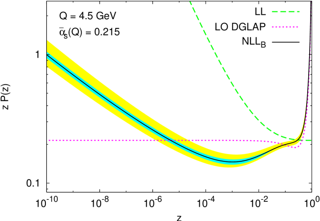
Figure 4: Small-$x$ $\mathrm{NLL_{B}}$ resummed splitting function, compared to the pure 1-loop DGLAP and the (fixed-coupling) LL BFKL splitting functions. The central $\mathrm{NLL_{B}}$ result corresponds to $x_{\mu}=1$, ${\bar{k}}=0.74\,\,\mathrm{GeV}$; the inner band is that obtained by varying ${\bar{k}}$ between $0.5$ and $1.0\,\,\mathrm{GeV}$, while the outer band corresponds to $\frac{1}{2}<x_{\mu}^{2}<2$.

Several features of the resummed splitting function are worth commenting and comparing with previous NLL calculations, including various types of resummations [10, 12, 13]. Firstly, at very large-$x$ it approaches the normal DGLAP splitting function. The momentum sum rule is satisfied to within a few parts in $10^{4}$. At moderately small-$x$ the splitting function is quite strongly suppressed with respect to the LL result and shows not a power growth, but instead a significant dip (of about $30\%$ relative to the LO DGLAP value, for $\bar{\alpha}_{s}=0.215$). Dips of various sizes and positions have been observed before in [13, 11, 25] though ours is significantly shallower than that found in [13] at NLL order and similar to that found in the $\omega$-expansion [16]. An interesting question concerns the impact of the dip on fits to parton distributions. Calculations in a (partially) RGI LL model [24] whose effective splitting function also has a dip, suggest that it is not incompatible with the available structure function data.

At very small-$x$ one finally sees the BFKL growth of the splitting function. We recall that the branch cut, present for a fixed coupling, gets broken up into a string of poles, with the rightmost pole located at $\omega_{c}$, to the left of the original branch point ($\omega_{s}$), $\omega_{s}-\omega_{c}\sim b^{2/3}\alpha_{s}^{5/3}$ [10]. The origin of this correction is similar to that of the $b^{2/3}\alpha_{s}^{5/3}$ contributions to $\omega_{\mathbb{P}}$ for cutoff regularisations [37]. The dependence of $\omega_{c}$ on $Q$ is shown in Fig. 3 together with its scale and IR regularisation dependence. It is slightly lower than the earlier determination in the $\omega$-expansion [10]. Both determinations are substantially below $\omega_{s}$, as expected.

4 Conclusions

In this letter we have outlined an approach to renormalisation-group improved NLL BFKL resummation that is convenient for numerical determination of the high-energy Green’s functions and splitting functions. This is an important step on the way to complete RGI NLL predictions for high-energy cross sections and small-$x$ structure function evolution.

We have discussed several important new results obtained within this approach. Most striking is the increase in the domain in $k$ and $Y$ that becomes perturbatively accessible once one includes subleading corrections. Even the amount of growth (number of ‘e-folds’) of the Green’s function that can be calculated perturbatively increases significantly.

Another result concerns the size of preasymptotic effects: for example, for the transverse scale studied in Fig. 1, BFKL growth sets in only for rapidities greater than $4$. Hence it is vital to study the full Green’s function rather than just the high-energy exponents discussed so far in the literature, and to include the physical impact factors [18, 19] along the lines suggested in[16].

In the collinear region, a key result is the practical demonstration of factorisation of the small-$x$ Green function, and the extraction of the resummed $P_{gg}$ splitting function. Here we obtain the high-energy exponent $\omega_{c}$, but we find that preasymptotic effects are again of fundamental phenomenological importance. As has been observed in an approach without renormalisation-group improvement [13], the main feature in today’s accessible $x$ range is a small-$x$ dip rather than growth (our dip is however much shallower). This phenomenon has yet to be fully understood, because several subleading effects are likely to come into play.

On the whole, the present work encourages us to trust resummed perturbative calculations for next generation accelerators, and shows that subleading contributions not only decrease high-energy exponents, but provide significant preasymptotic effects.

References

-
[1]
L.N. Lipatov, Sov. J. Nucl. Phys. 23 (1976) 338;
E.A. Kuraev, L.N. Lipatov and V.S. Fadin, Sov. Phys. JETP 45 (1977) 199;
I.I. Balitsky and L.N. Lipatov, Sov. J. Nucl. Phys. 28 (1978) 338. -
[2]
V.S. Fadin, M.I. Kotsky and R. Fiore, Phys. Lett. B 359 (1995) 181;
V.S. Fadin, M.I. Kotsky and L.N. Lipatov, BUDKERINP-96-92, hep-ph/9704267; V.S. Fadin, R. Fiore, A. Flachi and M.I. Kotsky, Phys. Lett. B 422 (1998) 287;
V.S. Fadin and L.N. Lipatov, Phys. Lett. B 429 (1998) 127.
- [3] G. Camici and M. Ciafaloni, Phys. Lett. B 386 (1996) 341; Phys. Lett. B 412 (1997) 396, [Erratum-ibid.Phys. Lett. B 417 (1997) 390]; Phys. Lett. B 430 (1998) 349.
- [4] J. Kwieciński, Z. Phys. C 29 (1985) 561; J.C. Collins and J. Kwieciński Nucl. Phys. B 316 (1989) 307.
- [5] L.N. Lipatov, Sov. Phys. JETP 63 (1986) 904.
- [6] G. Camici and M. Ciafaloni, Phys. Lett. B 395 (1997) 118.
- [7] G. Camici and M. Ciafaloni, Nucl. Phys. B 496 (1997) 305; Erratum-ibid. Nucl. Phys. B 607 (2001) 431.
- [8] G.P. Salam, JHEP 9807 (1998) 19.
- [9] M. Ciafaloni, D. Colferai, Phys. Lett. B 452 (1999) 372.
- [10] M. Ciafaloni, D. Colferai and G.P. Salam, Phys. Rev. D 60 (1999) 114036.
- [11] G. Altarelli, R.D. Ball and S. Forte, Nucl. Phys. B 575 (2000) 313; Nucl. Phys. B 599 (2001) 383.
- [12] G. Altarelli, R.D. Ball and S. Forte, Nucl. Phys. B 621 (2002) 359.
- [13] R.S. Thorne, Phys. Rev. D 64 (2001) 074005; Phys. Lett. B 474 (2000) 372.
- [14] C.R. Schmidt, Phys. Rev. D 60 (1999) 074003; MSUHEP-90416, hep-ph/9904368.
- [15] S.J. Brodsky, V.S. Fadin, V.T. Kim, L.N. Lipatov and G.B. Pivovarov, JETP Lett. 70 (1999) 155.
- [16] M. Ciafaloni, D. Colferai, G.P. Salam and A.M. Stasto, in preparation.
-
[17]
S. Catani, M. Ciafaloni and F. Hautmann,
Phys. Lett. B 242 (1990) 97;
S. Catani, M. Ciafaloni and F. Hautmann, Nucl. Phys. B 366 (1991) 135;
J. C. Collins and R. K. Ellis, Nucl. Phys. B 360 (1991) 3. Nucl. Phys. B 360 (1991) 3 -
[18]
J. Bartels, S. Gieseke and C.-F. Qiao, Phys. Rev. D 63 (2001) 056014;
Erratum-ibid. Phys. Rev. D 65 (2002) 079902;
J. Bartels, S. Gieseke and A. Kyrieleis, Phys. Rev. D 65 (2002) 014006;
J. Bartels, D. Colferai, S. Gieseke and A. Kyrieleis, Phys. Rev. D 66 (2002) 094017. - [19] J. Bartels, D. Colferai and G.P. Vacca, Eur. Phys. J. C 24 (2002) 83; hep-ph/0206290.
-
[20]
V.N. Gribov and L.N. Lipatov, Sov. J. Nucl. Phys. 15 (1972) 438;
G. Altarelli and G. Parisi, Nucl. Phys. B 126 (1977) 298;
Yu.L. Dokshitzer, Sov. Phys. JETP 46 (1977) 641. - [21] G. Bottazzi, G. Marchesini, G.P. Salam and M. Scorletti, Nucl. Phys. B 505 (1997) 366.
- [22] M. Ciafaloni, Nucl. Phys. B 296 (1988) 49.
- [23] B. Andersson, G. Gustafson and J. Samuelsson, Nucl. Phys. B 467 (1996) 443.
- [24] J. Kwiecinski, A. D. Martin and A.M. Stasto, Phys. Rev. D 56 (1997) 3991.
- [25] M. Ciafaloni, D. Colferai and G.P. Salam, JHEP 0007 (2000) 054.
- [26] M. Ciafaloni, D. Colferai, G.P. Salam and A.M. Stasto, Phys. Lett. B 541 (2002) 314.
- [27] Y.V. Kovchegov and A.H. Mueller, Phys. Lett. B 439 (1998) 428.
- [28] N. Armesto, J. Bartels and M.A. Braun, Phys. Lett. B 442 (1998) 459.
- [29] E.M. Levin, Nucl. Phys. B 453 (1995) 303; Nucl. Phys. B 545 (1999) 481.
- [30] M. Ciafaloni, A.H. Mueller and M. Taiuti, Nucl. Phys. B 616 (2001) 349.
- [31] M. Ciafaloni, D. Colferai and G. P. Salam, JHEP 9910 (1999) 017.
- [32] OPAL Collaboration (G. Abbiendi et al.), Eur. Phys. J. C 24 (2002) 17.
- [33] L3 Collaboration (P. Achard et al.), Phys. Lett. B 531 (2002) 39.
-
[34]
V. Del Duca and C. R. Schmidt,
Phys. Rev. D 51 (1995) 2150;
L. H. Orr and W. J. Stirling, Phys. Rev. D 56 (1997) 5875;
J. Kwiecinski and L. Motyka, Eur. Phys. J. C 18 (2000) 343;
J. R. Andersen, V. Del Duca, S. Frixione, C. R. Schmidt and W. J. Stirling, JHEP 0102 (2001) 007;
V. Del Duca, F. Maltoni and Z. Trocsanyi, JHEP 0205 (2002) 005. - [35] M. Ciafaloni, D. Colferai, G.P. Salam and A.M. Stasto, Phys. Rev. D 66 (2002) 054014.
- [36] D.A. Ross, Phys. Lett. B 431 (1998) 161.
- [37] R.E. Hancock and D.A. Ross, Nucl. Phys. B 383 (1992) 575; Nucl. Phys. B 394 (1993) 200.