Matching NLO QCD and Parton Showers in Heavy Flavour Production111Work supported in part by the UK Particle Physics and Astronomy Research Council and by the EU Fourth Framework Programme ‘Training and Mobility of Researchers’, Network ‘Quantum Chromodynamics and the Deep Structure of Elementary Particles’, contract FMRX-CT98-0194 (DG 12 - MIHT).
Abstract:
We apply the MC@NLO approach to the process of heavy flavour hadroproduction. MC@NLO is a method for matching next-to-leading order (NLO) QCD calculations and parton shower Monte Carlo (MC) simulations, with the following features: fully exclusive events are generated, with hadronisation according to the MC model; total rates are accurate to NLO; NLO results for distributions are recovered upon expansion in ; hard emissions are treated as in NLO computations while soft/collinear emissions are handled by the MC simulation, with the same logarithmic accuracy as the MC; matching between the hard and soft regions is smooth, and no intermediate integration steps are necessary. The method was applied previously to the hadroproduction of gauge boson pairs, which at NLO involves only initial-state QCD radiation and a unique colour structure. In heavy flavour production, it is necessary to include contributions from final-state QCD radiation and different colour flows. We present illustrative results on top and bottom production at the Tevatron and LHC.
Cavendish–HEP–03/03
CERN–TH/2003–102
GEF–TH–5/2003
1 Introduction
The process of heavy flavour production in hadron collisions is a valuable testing-ground for perturbative QCD, since the high scale set by the quark mass should ensure that perturbative calculations are reliable. The prediction of cross sections and final-state distributions in heavy flavour production is also important for the design of collider experiments and new particle searches, since this process gives rise to irreducible backgrounds to many types of new physics.
Up to now, the theoretical emphasis has been on next-to-leading order (NLO) calculations of total rates, single-inclusive distributions, and heavy quark-antiquark correlations, sometimes with resummation of higher-order contributions that are enhanced in certain kinematic regions. However, for many purposes, such as studies of backgrounds to new physics, one needs a more complete characterization of the final state. This is provided by a Monte Carlo event generator program, which combines a calculation of the hard production process with a parton shower simulation and a hadronization model, to yield an approximate but realistic hadron-level event structure.
The problem with existing Monte Carlo event generators is that they are based on a leading-order (LO) calculation of the production process combined with a leading-logarithmic (LL) treatment of higher orders via the parton shower approximation. It has proved highly non-trivial to incorporate the benefits of NLO calculations into event generators, since the parton showers include parts of the NLO corrections, which should not be double-counted. On the other hand, the parton showers cannot be omitted, since they provide a reliable description of how final state hard partons evolve into QCD jets. Furthermore, any viable hadronization model operates on the multiparton states that are created by showering.
A recent proposal for combining NLO calculations and parton showers is the so-called MC@NLO approach, introduced in ref. [1] (hereafter referred to as I). It is based on the highly successful subtraction method for NLO calculations. The basic idea is to modify the subtraction to take into account the terms that are generated by the parton shower. This results in a set of weighted LO and NLO parton configurations that can be fed into the parton showering generator without fear of double counting. Each weight distribution is well-behaved in the sense that it has no divergences or pathological tails that would lead to Monte Carlo inefficiency. However, in order to reproduce the NLO corrections fully, some of the configurations have negative weights. Event unweighting can still be achieved efficiently, if desired, by generating a small fraction of ‘counter-events’ that contribute with equal but opposite weight to events in all distributions.
The MC@NLO method was worked out in detail in I for processes in which, at the Born level, there are no coloured partons in the final state. An important example is gauge boson pair production, for which a wide range of MC@NLO predictions were presented there. To deal with the process of heavy quark production we must take into account QCD radiation from final-state partons, in this case the heavy quarks themselves. A further new complication is the possibility of different colour flows.
We shall see that no difficulties of principle arise from these complications. The only new task, albeit a laborious one, is to calculate precisely what the shower Monte Carlo is doing at NLO, in order to compute the modified subtractions correctly. In our case we use the HERWIG shower Monte Carlo [2], the relevant features of which are summarized in Appendix A.
In the following section we review the main features of the MC@NLO approach. Then, in sect. 3, we discuss the partonic processes that contribute to heavy flavour production in standard Monte Carlos and in MC@NLO, and we define the kinematic variables for the corresponding and processes. In order to compute the Monte Carlo subtraction terms that form the basis of the MC@NLO method, we have first to relate these variables to those used in the HERWIG program. This is done in sect. 4. Next we write down, in sect. 5, the approximate particle production cross sections generated by the HERWIG parton showering algorithm, which are then used to construct the Monte Carlo subtraction terms for heavy flavour production. Technical details of this procedure are given in Appendix B. Inserting the subtraction terms in the formulae reviewed in sect. 2 enables us to generate parton configurations that can be fed into the shower Monte Carlo without any double counting of NLO contributions. In order for the HERWIG Monte Carlo to operate correctly we have to assign a colour flow to each configuration; this and other details of the implementation are explained in sect. 6.
We present the predictions of MC@NLO for top quark production in sect. 7. The case of bottom is much more involved than that of top. Problems affecting -physics simulations with standard Monte Carlos are reported in sect. 8.1; in sect. 8.2, we discuss some of the features of MC@NLO in production, and in particular the treatment of large logarithms of , the ratio of the quark transverse momentum to its mass; in sects. 8.3 and 8.4 we present MC@NLO predictions for correlations and single-inclusive distributions respectively, and compare them to HERWIG and NLO results. Finally, conclusions and future prospects are presented in sect. 9.
2 Review of MC@NLO approach
The MC@NLO formalism is defined in eq. (4.22) of I, which we denote by eq. (I.4.22). We rewrite that equation in the following, fully equivalent, form:
| (1) | |||||
The quantities , , and appearing in eq. (I.4.22) have been replaced here by (the MC@NLO generating functional), (the MC generating functional when starting from a hard subprocess), and (the MC generating functional when starting from a hard subprocess) respectively. This renders more transparent the fact that the dependence upon the observable in eq. (I.4.22) is only formal, and that the MC@NLO generates events without reference to any observable. We refer the reader to for the definitions of all the terms appearing in eq. (1); however, the precise details will not be relevant here. In what follows, we shall limit ourselves to describing the basic features of eq. (1), and their role in the implementation of heavy flavour production in MC@NLO.
We start by recalling that the definition of MC@NLO is derived from the expectation value , computed at the NLO, of a generic observable , eq. (I.4.19). This can be read off from eq. (1) simply by removing the MC subtraction terms , and by replacing with , where is the observable computed in an -body final-state configuration (). The NLO expression for is an integral over the momentum fractions and of the incoming partons, and three-body phase-space variables . Each point in the integration range thus corresponds to a kinematic configuration (called hereafter). Furthermore, a definite configuration is chosen (called hereafter), according to a mapping which we denote by . The weight associated with is given by the real-emission matrix element; the sum of all the remaining contributions to the NLO cross section (namely, the Born term, the virtual term, the soft and collinear counterterms, and the finite remainders of the initial-state collinear singularity subtractions) constitutes the weight associated with . One can prove that it is always possible to cast any expectation value in this form (see , sects. 4.4 and A.4), through a formal procedure that we call event projection. It should be clear that event projection does not imply any approximation, and that its specific form depends on the choice of . In the context of a pure NLO computation, this choice is arbitrary, and its freedom has been used in the past [3] to improve the convergence of the numerical integration procedure. On the other hand, when defining an MC@NLO it is the MC itself that dictates the form of .
We suppose now to have chosen a map , and to have performed event projection on an NLO cross section. For each point we get a pair of kinematic configurations, and . Instead of using these configurations for defining the observable , as in the NLO computation of , we feed them into an MC, where they are treated as initial conditions for shower evolution. This corresponds to defining the MC@NLO as in eq. (1), except for the MC subtraction terms which are omitted. However, this naive attempt fails (see , sect. 3.3.1). Basically, when evolving configurations the shower reproduces some of the configurations, which are therefore double counted. The idea of modified subtraction, upon which the MC@NLO approach is based, is to subtract these double-counted configurations at the level of short-distance cross sections. This is the role of the MC subtraction terms which appear in eq. (1); they come in pairs, since they have to account for both the emission and the non-branching probabilities in the MC. The MC subtraction terms act as local counterterms in eq. (1), and this implies that the weight distributions for and configurations (the terms multiplying and respectively, see also eq. (I.4.23) and eq. (I.4.24)) are separately convergent, thus allowing event unweighting as is customary in MC simulations.
The MC subtraction terms are obtained by formally expanding the MC results to the first non-trivial order in , which corresponds to an configuration. Typically, has the form of a hard, cross section, times a kernel which describes (the first) parton branching. The shower algorithm fully specifies how to determine the configuration, given the hard configuration and the values of the showering variables. Thus, it implicitly defines a map between the and configurations. We choose , used in event projection, to coincide with this map. Notice that this is possible only because the shower algorithm is independent of the hard process.
In summary, the main steps that have to be taken in order to construct an MC@NLO are the following.
-
i)
Determine .
-
ii)
Write the NLO cross section for the relevant production process, and perform event projection on it, using the map found in i).
-
iii)
Define the MC subtraction terms, and insert them into the expression for the NLO cross section.
Of the three steps above, only ii) depends on the process in a non-trivial way. The implementation of event projection requires a detailed knowledge of the formalism adopted to write the cross section to the NLO accuracy; an explicit example of such a procedure has been given in , but different prescriptions are clearly possible. On the other hand, step i) is strictly process-independent, and thus can be determined once and for all. However, depends on the particular shower algorithm adopted, and therefore different MC’s define different maps. Finally, step iii) is process dependent, but only through the hard cross sections that appear in a factorized form in the MC subtraction terms, i.e. at the LO level, which is fairly simple to deal with. The part of the MC subtraction term which describes the first branching depends only on the shower algorithm, and can therefore be studied with full generality.
The definition of the MC subtraction terms is in fact one of the main goals of the present paper; final-state emissions are considered here for the first time, since they were not relevant to the production of vector boson pairs considered in . Also, the formulae presented in for initial-state emissions will be generalized here to account for colour structures more complicated that those of . These results will allow an almost straightforward definition of the MC subtraction terms for any production process. A subtle point concerns the interplay between initial- and final-state emissions, and its impact on the definition of -event contribution to MC@NLO. This issue is discussed in Appendix B.
3 Heavy quark production
3.1 Contributing processes
In the MC@NLO approach, the Monte Carlo is not involved in the generation of the hard process which, apart from the modified subtraction, is treated as in standard NLO codes. It follows that the partonic production processes that we need consider are
| (2) |
at and , and
| (3) |
at . As discussed previously, the contributions in eq. (2) generate (some of) the configurations in eq. (3) through parton showering, but MC@NLO is defined in such a way to avoid any double counting. The processes in eq. (2) are traditionally classified as flavour creation (FCR hereafter) to distinguish them from the so-called flavour excitation (FEX hereafter) processes
| (4) |
where charge-conjugate processes are understood to be included. In the case of FEX processes, it is implicitly assumed that the relevant heavy flavour is already present in the parton distribution functions (PDFs) of the incoming hadrons.
In standard Monte Carlo, both FCR and FEX matrix elements are used in the generation of the hard processes.222FEX is not relevant to top production at realistic collider energies. This is not the case in NLO computations, since the partons which initiate the hard processes are treated as massless, understanding that their actual mass is negligible with respect to the hard scale of the process, in this case the heavy quark mass . This forbids the presence of heavy quarks in the initial state. Furthermore, if we use NLO matrix elements in the generation of the hard process, as in MC@NLO, the distinction between FCR and FEX becomes ambiguous. For example, the NLO FCR process has a contribution from initial-state quasi-collinear gluon splitting, , followed by the LO FEX process . Since initial-state quasi-collinear gluon splitting forms part of the evolution of the PDFs of the incoming hadrons implemented through parton showers, we are in danger of double-counting if we include both LO FEX and NLO FCR processes in MC@NLO. On the other hand, this example explains why FEX processes are considered in standard Monte Carlo: they allow one to include some of the features that could not be included by shower evolution initiated by FCR processes. We also point out that the process , which we include in the MC@NLO, generates certain kinematic configurations that can be equivalently produced starting from a hard process followed by final-state gluon splitting . The gluon splitting mechanism (GSP hereafter) is known to be important in bottom production, giving the dominant contribution to those configurations in which and are close in phase space (which is important not only for the study of correlations, but also in -jet physics), and non-negligible contributions to single-inclusive distributions in the intermediate- region.
Flavour excitation and gluon splitting pose a couple of non-trivial problems in standard Monte Carlo event generators.333For a discussion of physics as described by Monte Carlo parton shower programs, see e.g. refs. [4, 5]. In FEX, the presence of a heavy quark in the initial state implies a direct dependence upon its PDF; in the small- region, i.e. close to threshold, it is unlikely that the treatment of the backward evolution performed by the parton shower will be compatible with what was implemented in the PDF evolution. Furthermore, the -channel singularity in the matrix elements requires the implementation of a cutoff (possibly an effective one, see app. A.1.2) which prevents the generation of events. Both features result in predictions which have a certain degree of implementation dependence. As far as GSP is concerned, the corresponding events are usually obtained by considering pure QCD events (i.e., with no heavy quark involved in the hard process, the generation of which also requires a cutoff), and selecting those in which at least one pair is obtained through showering, a very inefficient procedure from the statistical point of view. More details will be given in sect. 8.1.
Worst of all, both FEX and GSP processes are well defined only in the case of large transverse momenta of the heavy quark. Their extrapolation to the low transverse momentum region can at best be considered a very rough model of higher-order heavy flavour production processes.
The implementation of heavy flavour production in MC@NLO helps to avoid some of these problematic features of the FEX and GSP processes. In the processes considered in NLO computations, eqs. (2) and (3), there is no such thing as direct dependence upon the heavy quark PDF, and singularities are cancelled at the level of short-distance cross sections, without the need to introduce unphysical parameters acting as cutoffs. Furthermore, one generates gluon splittings with 100% efficiency, since they are included in the matrix elements. Clearly, the presence of negative weights in MC@NLO degrades the statistics, but (at least with the fraction of negative weights we find in our implementation) the overall efficiency is still larger than that required to obtain a useful gluon-splitting sample with the usual Monte Carlo method.
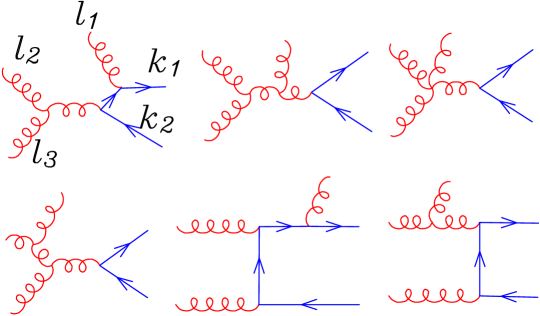
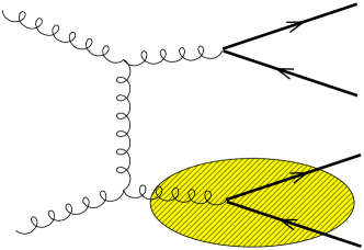
However, an MC@NLO based on the hard processes of eqs. (2) and (3) cannot account for all the contributions generated by FEX and GSP. For example, MC@NLO does not include the diagrams in which a gluon, rather than a heavy quark, is emitted in the first backward branching of the heavy quark entering a FEX hard process. Similarly, MC@NLO does not include those GSP diagrams in which the gluon emits another gluon before splitting. Examples of omitted contributions are shown in fig. 1.

The absence of such contributions is not surprising: the terms missed by the MC@NLO are part of those relevant to the region of large heavy-quark transverse momenta (large ), where the quark mass no longer sets the hard scale. In this region, the NLO computation is not expected to give sensible results, since large logarithms need to be resummed to all orders. For single-inclusive observables, techniques are known for resumming these large logs (to NLL accuracy), and for matching the resummed result to the NLO one (for example, FONLL [6]). However, there is at present no known way of extending such a procedure to the fully exclusive case that would be needed in order to include it in MC@NLO. This problem is relevant, for example, to bottom production at the Tevatron. In sect. 8.2 we shall show that MC@NLO gives in practice a sensible answer also in this case, since these enhanced high- effects are not so large in the kinematic region of practical interest.
3.2 processes
In this and in the following section, we introduce the notation that we shall use in order to describe the hard processes in eqs. (2) and (3).
We denote variables relating to the FCR processes of eq. (2) by barred symbols: represent the incoming (massless) momenta and the outgoing heavy quark and antiquark (mass ) momenta. The momentum fractions of the incoming partons are denoted by , i.e.
| (5) |
where are the beam momenta, and the invariants by
| (6) |
Then and , where is the overall c.m. energy squared. In the c.m. frame of the process, we can write
| (7) |
where
| (8) |
We also introduce the c.m. scattering angle and heavy quark velocity
| (9) |
so that
| (10) |
The hard scattering Born cross section is then
| (11) |
where
| (12) |
being the spin- and colour-averaged Born matrix element squared for the process , times the flux factor:
| (13) | |||||
| (14) |
3.3 processes
For the FCR processes of eq. (3) we use unbarred symbols: for the incoming (massless) momenta, for the outgoing heavy quark and antiquark momenta, respectively, and for the momentum of the emitted (massless) parton. We denote the momentum fractions of the incoming partons by , i.e.
| (15) |
and the invariants by
| (16) |
so that . We also introduce
| (17) |
and
| (18) |
but these are not independent variables since
| (19) |
This notation is summarized and compared with that of ref. [3] in table 1.
| Label | Invariant | Ref. [3] | Relation |
|---|---|---|---|
4 Relating NLO and MC kinematics
As discussed in sect. 2, the implementation of MC@NLO requires a detailed knowledge of the relation between () and () kinematic configurations. Also, for the integration of the MC subtraction terms over the three-body phase space, as prescribed in eq. (1), we need to express the MC showering variables in terms of the phase-space variables. We solve both problems in the same way, presenting the invariants and showering variables as functions of the three-body invariants. The latter will eventually be computed by means of the three-body phase-space variables; however, in this section we shall not introduce any explicit phase-space parametrization, and the results are therefore fully general.
A shower Monte Carlo program generates arbitrarily complicated multiparton configurations by an iterative process of parton emission, starting from the coloured external lines of a hard subprocess. In the hard subprocess these external lines are treated as being on mass-shell, but the showering process may drive them off the mass shell, and the kinematics have to be adjusted to restore energy-momentum conservation. This process is called momentum reshuffling; the way it is implemented in the HERWIG program is described in app. A.2.4. The relationship between and kinematics discussed in the following subsections depends upon the particular implementation of momentum reshuffling.
4.1 Relating and kinematics
The relationship between the variables of the hard process, and the variables which result after one parton emission is not simple, owing to momentum reshuffling. In particular, since initial- and final-state showers are treated differently in the reshuffling, it depends on whether the parton emission is from an incoming or outgoing parton.
We consider the case of FCR with momenta and momenta . The way in which we relate the kinematics of the and processes is by solving for the invariants and momentum fractions in terms of the invariants and momentum fractions . In terms of the c.m. frame variables defined in eq. (7), this amounts to finding , , and .
It should be noted that the kinematics used in parton shower Monte Carlos generally involve cutoffs that operate like effective light quark and gluon masses. We can ignore these cutoffs in computing the Monte Carlo subtraction terms since they only give rise to power-suppressed corrections, comparable to hadronization effects, in physical distributions. This point was discussed in I, sect. B.3.
4.1.1 Final-state emission
Suppose a gluon is emitted from the heavy quark. The final state is then formed by the heavy quark jet (i.e. the heavy quark plus the emitted gluon) and the heavy antiquark. The three-momenta of the antiquark and of the heavy quark jet are rescaled by a common factor in order to restore energy conservation, according to the prescription described in appendix A.2.4. The heavy antiquark has momentum (in the hard process c.m. frame)
| (20) |
where and is the rescaling factor, given by the energy conservation constraint,
| (21) |
Hence for final-state emission from the heavy quark we find
| (22) |
where is the velocity of the heavy antiquark in the heavy quark-antiquark c.m. frame,
| (23) |
For emission from the heavy antiquark, the labels 1 and 2 are interchanged, so the relation between the and invariants depends on which outgoing parton emits the gluon. We label the invariants as , , etc., according to which parton is the emitter. Then we have explicitly
| (24) |
where
| (25) |
Note that in the soft limit (, , ) we have and as expected.
The incoming parton momenta are not affected, so , and . Thus the incoming momentum fractions are unchanged by final-state emission:
| (26) |
The formulae presented here can also be used for the branchings of massless partons; one simply lets , , . In such cases, collinear limits must also be considered. When a gluon is emitted collinearly by the heavy quark (, , , ) we have , . For a collinear emission by the heavy antiquark (, , , ) we have , .
4.1.2 Initial-state emission
In the case of emission from the incoming partons, the invariant mass of the heavy quark pair is not changed by momentum reshuffling, so
| (27) |
However, the pair receives longitudinal and transverse boosts, as described in app. A.2.4. To relate the other invariants, we consider the heavy quark momentum difference. In the c.m. frame, it is
| (28) |
Since this has no energy component, the effect of the longitudinal boost is simply to rescale the longitudinal component by the boost factor
| (29) |
The transverse boost does not change the longitudinal component, so
| (30) |
We can extract the longitudinal components using the combination
| (31) |
Hence
| (32) |
where
| (33) |
Expressing everything in terms of invariants, we therefore have for initial-state emission
| (34) |
where for future reference we have defined
| (35) |
Note that in this case the result is independent of which incoming parton emits. However, for consistency we label or according to whether parton 1 or 2 is emitting. Thus we have explicitly
| (36) |
Again in the soft limit (, , ) we have and as expected. In the case of collinear emission from leg 1 (, , , , ) we have , . For a collinear emission from leg 2 (, , , , ) we also have , .
To relate the incoming momentum fractions, we note that in this case eq. (27) applies, and therefore instead of eq. (26) we have
| (37) |
The values of and separately depend on the momentum reshuffling scheme, as explained in app. A.2.4:
-
•
In the -scheme the longitudinal momentum of the heavy-quark pair is preserved, which means that
(38) and hence
(39) where are given by eq. (35). Note that eq. (39) coincides with eq. (I.A.47); this is to be expected, since the details of the hard process are irrelevant in the determination of the ’s.
-
•
In the -scheme the rapidity of the heavy-quark pair is preserved, which implies
(40) and hence
(41) which corresponds to eq. (I.A.42).
4.2 Relating HERWIG variables to invariants
When relating the HERWIG showering variables to the kinematics of the hard process, we must again take careful account of which quantities are preserved under momentum reshuffling.
4.2.1 Final-state emission
For emission of a gluon from the outgoing heavy quark in the FCR processes, the HERWIG variables are the angular variable and the energy fraction , all energies being evaluated in the showering frame where or as discussed in app. A.2.1. The invariant quantities are the jet virtuality
| (42) |
and the “+” momentum fraction of the gluon with respect to the jet axis,
| (43) |
where is the heavy-quark jet velocity in the showering frame
| (44) |
and is a lightlike vector along the direction of the heavy antiquark in the heavy quark-antiquark c.m. frame:
| (45) |
where is given by eq. (23). Inserting eq. (45) into eq. (43), we find
| (46) |
Solving eqs. (42), (43) and (46) for and with as given in eq. (4.1.1), we obtain and , corresponding to emission from the heavy quark with the -flow colour structure as defined in app. A.1.3. Similarly, solving with , as appropriate to the -flow, gives and . We find that
| (47) | |||||
| (48) |
where for . Interchanging the labels 1 and 2 and using instead of gives and , corresponding to emission from the heavy antiquark.
Note that the transverse momentum of the emitted gluon relative to the jet axis is where
| (49) |
and thus at small values of and , where is the HERWIG evolution variable.
4.2.2 Initial-state emission
In the case of an initial-state jet, the jet axis coincides with the beam axis and so the jet invariants are simpler than in the final-state case. For emission from parton 1, the jet virtuality is
| (50) |
and the “+” component of the gluon momentum is444Note that eqs. (50) and (51) are equivalent to eq. (I.A.67) and eq. (I.A.68), if we set .
| (51) |
Solving eqs. (50) and (51) for and with or as given in eq. (4.1.2), we obtain and , corresponding to emission from incoming parton 1 with these initial conditions. In the case of emission from an initial-state gluon, we also have the possibility that (see app. A.1.3), and we denote the corresponding variables by and . Then we can write the solutions explicitly as
| (52) | |||||
| (53) |
where for .
For emission from incoming parton 2, the variables and are interchanged. We denote the corresponding solutions by and .
4.3 Dead regions
The parton shower initial conditions imply that gluon radiation is confined to angular regions (cones) specified by the colour flow. This represents an approximate treatment of the destructive interference due to colour coherence. The dead regions outside the cones can be found from the above mapping of the HERWIG shower variables onto invariants.
4.3.1 Final-state emission
For final-state jets the kinematic region available for gluon emission is
| (54) |
However, the radiation in the forward direction is suppressed dynamically for and therefore in HERWIG the region used (neglecting the gluon effective mass cutoff) is
| (55) |
The scale is given by or or , depending on the colour flow (see app. A.2.1). Thus all cases can be represented by the situation for , with when and when .
It is convenient to express the jet regions in terms of the Dalitz plot variables of the final state,
| (56) | |||||
Then for emission from the heavy quark we have
| (57) | |||||
| (58) |
where and are related to the HERWIG variables and by eqs. (42) and (43). For emission from the heavy antiquark, the variables and are interchanged.

The boundaries of the quark and antiquark jet regions of the Dalitz plot are shown in fig. 2. Note that there is an overlap in the soft region for . The boundary of the physical region is also shown (short-dashed). We see that there is a dead region in which hard, non-collinear gluon emission is missed by the HERWIG shower algorithm, and also narrow near-collinear dead regions, where emission is forbidden in order to simulate the dynamical suppression of collinear emission from the heavy quarks, as discussed above.
4.3.2 Initial-state emission
In the case of an initial-state jet, the allowed region is since now [7]. The conventional variables are which give the heavy diquark mass and the emission angle of the gluon in the partonic c.m. frame. For emission from incoming parton 1 we find:
| (59) |
For emission from parton 2, and are interchanged, i.e. . Inserting in eqs. (50)–(51) then gives the boundaries of the jet regions in the plane.

The jet boundaries are shown in fig. 3. Note that there is again an overlap in the soft region for . There are no collinear dead regions, because the incoming partons are treated as massless.
5 MC cross sections expanded to NLO
In this section, we present the cross section that we would obtain by keeping the first non-trivial order in the expansion of the HERWIG Monte Carlo result. This quantity, which we denote by , is directly related to the MC subtraction terms that enter the definition of MC@NLO. We shall not give here the rather technical details of the construction of the MC subtraction terms, which we report in app. B. We shall limit ourselves to highlighting the main differences with respect to , which result from the more complicated singularity and colour structure of the heavy flavour cross section.
The result we are seeking can be written as follows:
| (60) |
where the first sum in eq. (60) runs over parton processes. The index runs over the emitting legs and, consistently with sect. 4.1.1 and 4.1.2, it assumes the values , , , and . The index runs over the colour structures, and it can take the values , , and (see sect. 4.2.1 and 4.2.2). Using the same formal expansion as in eq. (I.A.58), we obtain
| (61) | |||||
| (62) | |||||
| (63) | |||||
| (64) |
In the case of , the sum of eqs. (61) and (62) coincides with eq. (I.A.58). The cases , and eqs. (63) and (64) were not considered in , since they correspond to colour flows not relevant to gauge boson pair production, and emissions from strongly-interacting final-state partons.
The short-distance cross sections in eqs. (61)–(64) have a form similar to eq. (I.A.63) and eq. (I.A.64), namely a factor depending on the HERWIG showering variables and , times a Born cross section. As discussed above, and , and the invariants and entering the Born cross sections, must be expressed in terms of the integration variables used in the NLO code. In the case of emissions from both the initial- and final-state partons, we have four pairs of functional relations between and and the NLO integration variables, corresponding to , , and (and analogously for ), given by eqs. (52,53) and (47,48). We have the following non-vanishing contributions:
initial state
| (65) | |||||
| (66) | |||||
| (67) | |||||
| (68) |
initial state
| (69) | |||||
| (70) | |||||
| (71) | |||||
| (72) |
where are the colour - and -flow contributions defined in eq. (92);
initial state
| (73) | |||||
| (74) | |||||
| (75) | |||||
| (76) | |||||
| (77) |
Note that in each equation the Born cross section or has to be computed using the relevant definitions of , and ; more details are given in app. B. The argument of used in the computation of these cross sections is the same one as that used in the computation of the NLO short-distance cross sections; as discussed in sect. 2, the generation of the hard process in MC@NLO has nothing to do with the analogous generation occurring in the MC. On the other hand, the factor of which explicitly appears in eqs. (65)–(77) is due to parton showering, and its argument should in principle be chosen according to eq. (90). However, the choice of this argument is strictly speaking a matter beyond NLO. This is discussed more fully in I, sect. B.3. As done there, for simplicity we choose the same scale as that used for NLO terms.
The analogous results for , , , and can easily be obtained from the equations above. The situation is summarized in table 2.
| , , | |||
| , , | |||
| , , |
6 Implementation of MC@NLO
The practical implementation of MC@NLO for heavy flavour production proceeds in a similar way to that for gauge boson pair production, described in sect. 4.5 of I. The integrals necessary to determine the required numbers of ( parton) and ( parton) configurations are computed according to eq. (I.4.23) and eq. (I.4.24), together with the corresponding equations in which the integrands are taken in absolute value. Configurations are generated according to the MC-subtracted weight distributions in eq. (1), and then unweighted with weight according to the sign of the weight, using the SPRING-BASES package [8]. Weighted events could also be generated, but this option is not implemented at the moment.
The selected configurations and their weights are written on a file which is input to the HERWIG event generator. HERWIG then performs the parton showering and hadronization as explained in app. A.2 and A.3 respectively. The generated events with weight +1 are to be treated as real events for the purposes of histogramming and/or detector simulation, whereas those with weight –1 (a fraction of the order of 10% for top and 20% for bottom) are “counter-events”, which must be treated as real events in detector simulation but have to be subtracted from histogram bins to which they contribute.
The only significant differences from the implementation of MC@NLO described in I are that a colour flow must be assigned to each parton configuration and that this flow, together with the event weight and the parton identities and momenta, are handled by the “Les Houches” generic user process interface [9]. Details of these two new features are given in the following subsections.
6.1 Colour flow assignment
The assignment of colour flows for configurations is done according to the HERWIG prescription explained in app. A.1.3: where the colour flow is ambiguous, it is assigned according to the limit. The same prescription is extended to configurations as follows.
Consider first the process . In the large- limit, the basic planar colour flow amplitude involving three gluons and a heavy quark-antiquark pair is depicted in fig. 4.

Double-directed lines are gluons, and single-directed lines are quarks. The momenta , and are all defined to be outgoing. In the notation of sect. 3.3, the six independent colour-ordered amplitudes for the process are obtained by replacing in all possible ways.
The amplitudes are easily computed from the large- limit Feynman rules, which amount to the following graphical prescriptions for the vertices:
| gluon: | (78) | ||||
| three gluons: | |||||
| four gluons: | (79) |
where all momenta and indices have to be assigned counterclockwise, and momenta are all incoming.
We define
| (80) |
the square of the sum of the amplitudes in fig. 5 in the large- limit, summed over spin and colours. The ordering of the momenta in the arguments of corresponds to the ordering of the colour connection, starting from the outgoing heavy quark.
There are two basic colour orderings for processes involving a gluon, a light quark-antiquark pair, and a heavy quark-antiquark pair. They are depicted in fig. 6.

Here we define two squared amplitudes
| (81) |
corresponding to colour flows (a) and (b) of fig. 6, respectively. The two squared amplitudes are related by charge conjugation
| (82) |
Notice that in our notation we call and the light flavour lines corresponding to an outgoing quark or antiquark respectively. The corresponding colour flow squared amplitudes for are obtained from the amplitudes of eq. (81) by the replacement , and . The squared amplitudes for the process are instead obtained with the replacement , , .
The correctness of our calculation of the colour flow amplitudes was checked by comparing the sum of all colour squared amplitudes with the known full squared amplitude, for very large values of .
As an example, consider the assignment of colour flow for the process . The configuration of momenta is chosen according to the full () expressions with modified subtraction as explained in sect. 2. Then the squared amplitudes for the large- colour flows in fig. 6 are computed:
| (83) |
The colour flows (a) and (b) are then assigned with probabilities
| (84) |
6.2 Interface to HERWIG MC
The colour flow selected as described above is encoded in a single integer IC which is written on a file together with the event weight and the parton momenta and identities. The possible values of the colour flow code IC and their meanings are given in app. C.
The file of parton configurations is read by HERWIG as input to the Les Houches generic user process interface [9]. A negative value of the process code IPROC signals to HERWIG that, instead of generating a partonic hard subprocess as outlined in app. A.1, it should load and use subprocess information in the Les Houches common blocks HEPRUP and HEPEUP.
First a file header is read by the interface subroutine UPINIT, which checks that the file has been generated with parameter values consistent with those set in this HERWIG run and initialises the run common block HEPRUP. The parton configurations are then read sequentially by the interface subroutine UPEVNT, which loads the event common block HEPEUP with all information necessary to generate an event, including the interpretation of the colour flow code IC as outlined above.
7 Results on top quark production
In this section we present results for top quark production, obtained with the MC@NLO implementation555A public version of the program is available on the MC@NLO web page http://www.hep.phy.cam.ac.uk/theory/webber/MCatNLO/. described above. We do not attempt here to give a phenomenological description that corresponds to a specific experimental configuration; rather, we wish to show the differences between MC@NLO, standard HERWIG MC, and NLO results. For this reason, we present distributions obtained either by integrating over the whole phase space, or else with cuts on the heavy quark variables, rather than on those of their decay products. We first show results for the LHC, i.e. for collisions at TeV. We set the top mass to GeV, and the renormalization and factorization scales equal to the top transverse mass, . We adopt the low- set of MRST99 parton densities [10], since this set has a value which is rather close to that used as HERWIG default. This value of ( MeV) is used for all our MC@NLO, MC, and NLO runs. In the case of standard HERWIG MC runs, we give each event (we generate unweighted events) a weight equal to , with the total number of events generated. For fully exclusive distributions with no cuts applied, this is equivalent to normalizing HERWIG results to the total NLO rate (with our choice of parameters, we obtain pb at the Tevatron, and pb at the LHC). All the MC@NLO and MC results (but not, of course, the NLO ones) include the hadronization of the partons in the final state.
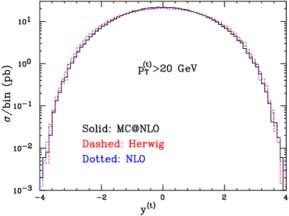
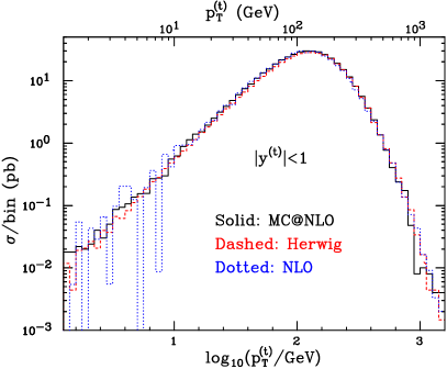
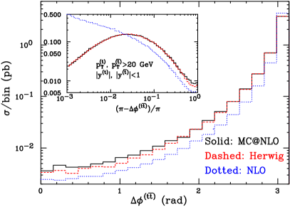
We present in fig. 7 the rapidity (left panel) and the transverse momentum (right panel) distributions of the top quark. The rapidity (transverse momentum) result has been obtained after applying the cut GeV (). The solid, dashed and dotted histograms show the MC@NLO, MC and NLO results, respectively. These distributions are fairly inclusive, and we expect them to be reliably predicted by NLO QCD in a wide range. From the figure, we see that the NLO and MC@NLO results are extremely close to each other in the whole ranges considered. HERWIG results are also fairly close to the NLO and MC@NLO ones, giving only a slightly broader rapidity distribution. The same pattern can be found for the invariant mass of the pair. We conclude that, for these kinds of observables, NNLO effects are very small, and NLO, MC and MC@NLO are almost equivalent. This also implies that any possible reshuffling of the momenta, due to the hadronization phase in MC@NLO, has negligible impact on the and . The right panel of fig. 7 also clearly shows a characteristic feature of the comparisons between MC@NLO and NLO results, namely that the former are numerically more stable than the latter. This feature, which is even more evident in the case of production, is due to the fact that, as eq. (1) documents, in MC@NLO all cancellations between large numbers occur at the level of short-distance cross sections, rather than in histograms as in the case of NLO computations.
We now turn to the case of more exclusive quantities, such as correlations between and variables. In fig. 8 we present the modulus of the vector sum of the transverse momenta of the and , which we denote by . NLO computations cannot predict this observable in the region , because of a logarithmic divergence for ; on the other hand, NLO is expected to give reliable predictions at large . The MC behaves in the opposite way; thanks to the cascade emission of soft and collinear partons, it can effectively resum the distribution around . However, its results are not reliable in the large- region, which is mainly populated by events in which a very hard parton recoils against the pair.
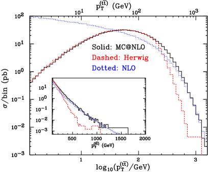
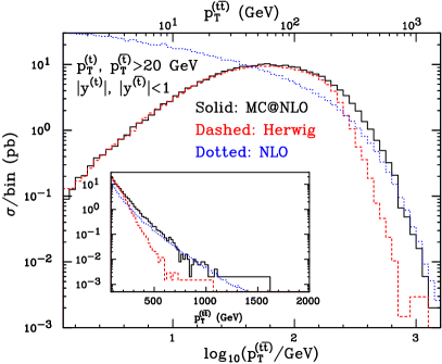
The complementary behaviour of the NLO and MC approaches can be seen clearly in fig. 8, regardless of the cuts on the rapidities and transverse momenta of the heavy quarks. In the tail of the distribution, the NLO cross section is much larger than the MC one, simply because hard emissions are correctly treated only in the former. The presence of the dead zones shown in figs. 2 and 3 makes it very difficult to generate a very hard parton recoiling against the pair in the MC, which therefore gives rates much below the NLO result in this region. For , the difference between the two histograms shows the effect of all-order resummation; clearly, no meaningful comparison between NLO and data can be attempted in this region. It is therefore reassuring that the MC@NLO result interpolates the MC and NLO results smoothly. In the small- region, the shape of the MC@NLO curve is identical to that of the MC result. This is evidence of the fact that MC and MC@NLO resum large logarithms at the same level of accuracy, as argued in I. When grows large, the MC@NLO tends to the NLO result, as expected. Again, hadronization has no significant impact on the system.
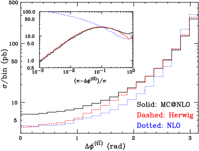
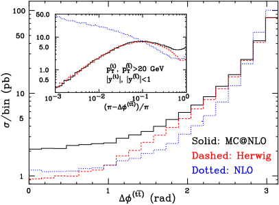
In fig. 9 we present the distribution of the difference between the azimuthal scattering angles (i.e., those in the plane transverse to the beam direction) of the and , which we denote by . This distribution cannot be reliably predicted by fixed-order QCD computations in the region ; in fact, the NLO prediction diverges logarithmically for . This can be seen in the insets of the plots, where the cross section has been plotted versus on a logarithmic scale, in order to visually enhance the region . We can see that in this region the MC@NLO and MC results have identical shapes, as in the case of the observable near zero discussed above. The other end of the spectrum, i.e. the tail , is populated by configurations in which a hard jet recoils against the pair, but also by configurations in which the and have small transverse momenta. The NLO calculation gives a good description of the former region, but not the latter, while the MC can treat reliably the latter region, but not the former. MC@NLO, on the other hand, is expected to handle both regions reliably, while still avoiding any double counting. We also notice that, when cuts on the transverse momenta of the heavy quarks are applied, the contribution from multiple soft or collinear emissions becomes less important, and so the MC does less well at , as may be seen in the right-hand panel of fig. 9.
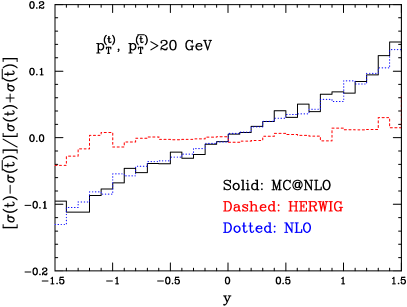
Corresponding results for Tevatron Run II ( at TeV) are shown in figs. 10-12. An interesting new feature of the top quark rapidity distribution is its forward-backward asymmetry, which cannot appear in collisions and is also absent in at the Born level, and hence also in the MC result. To document this, we plot in the left panel of fig. 10 the rapidity asymmetry rather than the rapidity itself; cuts GeV have been imposed. We see a fair agreement between MC@NLO and NLO, whereas HERWIG predicts an asymmetry compatible with zero.
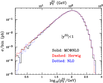
In the right panel of the same figure, the top quark transverse momentum (with a cut) is shown. As in the case of LHC, we see no substantial differences between NLO, MC@NLO and HERWIG.
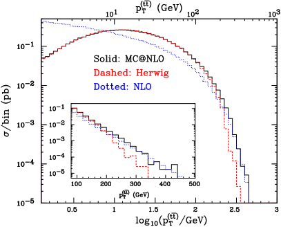
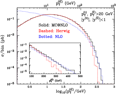
The picture for (fig. 11) is broadly similar to that at the LHC, except for the reduced tail at high : the MC@NLO prediction makes a smooth transition from the NLO to the resummed MC form as decreases.
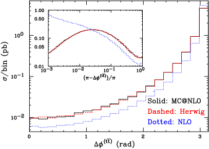
The situation for , on the other hand, is slightly different. At Tevatron energies the influence of hard emissions is not so strong as at the LHC. Consequently (see fig. 12) the MC and MC@NLO predictions coincide quite closely over the whole range of , whereas the NLO remains lower, regardless of whether or not cuts are applied.
8 Results on bottom quark production
In the case of bottom production, many complications arise that are not present in top production. In a standard Monte Carlo, all of the three mechanisms discussed in sect. 3.1, namely flavour creation (FCR), flavour excitation (FEX), and gluon splitting (GSP), need to be considered; they have rather different kinematic signatures, and they are dominant in different regions of the phase space. From the point of view of perturbative computations, bottom cross sections are characterized by a fairly large value of the coupling constant, which implies sizable K factors; also, the importance of large logarithmic terms arising at all orders is manifest in many observables, and suitable resummations are often necessary for sensible comparisons with data.
As in the case of top production, we shall not attempt here to discuss the phenomenological implications of our findings. We shall rather emphasize the kind of problems encountered in -physics simulations with standard MC’s, and the way in which MC@NLO solves some of them. Comparisons between MC@NLO and NLO results will also be presented here. We shall not discuss the well-known limitations of fixed-order computations, but refer the reader to ref. [11] for further details. Unlike the case of top production, in physics we can compare MC@NLO results with MC and NLO ones either for quarks or for -flavoured hadrons. The former option is clearly preferable, if we aim at understanding the extent of the validity of the MC@NLO approach, and the improvements with respect to traditional formalisms. Technically, in MC@NLO and in HERWIG we define the -quark level as the stage which comes immediately before the gluon-splitting phase,666This gluon splitting is non-perturbative, and it has nothing to do with the perturbative branching of a gluon which takes place during a shower; see app. A.3.1 for more details. corresponding to HERWIG status code ISTHEP=2.
The results presented in this section have been obtained at the Tevatron Run II ( at TeV), for a bottom mass of 5 GeV. The other parameters have been chosen as in sect. 7. In order to simplify the analysis procedure, pair observables are defined by considering all possible pairs in the event, regardless of their charge. Thus, in HERWIG and MC@NLO , , and pairs are treated on an equal footing (at the NLO, one has just one pair), and will collectively be denoted as pairs. From the practical point of view this detail is almost irrelevant, since we find that the probability of having more than two ’s in an event with at least two ’s is of the order of 0.1%.
8.1 -production issues in HERWIG
We start by discussing the problems arising in the simulation of production with HERWIG. We stress that similar problems are present in any standard parton shower MC. As we discussed in sect. 3.1, FEX and GSP contributions are considered in heavy flavour production simply because FCR alone is not capable of describing the kinematics of observed events. It should be noted that FEX and GSP are somewhat anomalous from the point of view of MC’s, since usually the simulation relevant to a given hard system involves the production of such a system at the level of hard process generation. This fact has profound consequences: MC’s cannot simulate small- production of heavy quarks, since FEX and GSP matrix elements are diverging for . This poses a practical problem, which is easily circumvented by cutting off the matrix element divergencies. In HERWIG, this is achieved by requiring the transverse momenta of the primary partons to be larger than a given quantity, called . In addition to this, HERWIG has an effective cutoff at the level of hard matrix elements for FEX processes, which prevents the generation of primary partons with even if (see app. A.1.2). In production, GSP processes also have an effective cutoff, but of a different nature. The probability of getting a showering scale large enough to produce a pair vanishes as in the hard process. Still, this doesn’t allow one to set in GSP, since the hard process is generated independently of the shower.
Although -channel singularities are cut off by , a problem of principle remains: if one interprets the output of a given showering event as a Feynman diagram, one obtains a contribution which in perturbation theory is only relevant in the large-momentum regime . Thus, strictly speaking one should run FEX and GSP, and keep only those events with a large- heavy quark. It is customary to ignore this problem, and to keep all the events generated. The results are in general biased by , and it is therefore necessary to insure that this bias does not affect the predictions in the kinematical regions of interest.
We have studied the bias due to the choice of by considering the GSP contribution. An analogous study can be done for the FEX contribution, but in this case the presence of an effective cutoff at the level of hard matrix elements complicates the discussion unnecessarily. We have considered the inclusive cross section, requiring
| (85) |
and the pair cross section, requiring
| (86) |
The results are presented in fig. 13; open points are HERWIG predictions for the corresponding value, and the solid lines are there just to guide the eye. The dotted line is the weighted average of the results for the pair cross sections obtained at , and 6 GeV.
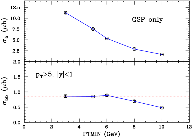
The lower panel of fig. 13 has an easy interpretation: for values smaller than 6 GeV, HERWIG predictions are independent of , i.e., they are not biased. Clearly, these values of are correlated to the choices of cuts made in eq. (86) and, to a smaller extent, to the fact that the observable chosen is fully inclusive. It seems however safe to choose GeV for studying any type of pair correlations with the cuts of eq. (86).
The upper panel of fig. 13 displays a less pleasant behaviour; no range in can be found where the inclusive- cross section is independent of . This happens because, at small but finite of the primary partons, HERWIG can choose a colour flow according to which the evolution scale is almost equal to . Thus, a gluon acquires a large enough virtuality to split into a pair. When boosted to the lab frame, one of the ’s can have a transverse momentum exceeding the cut (the probability for this to happen is small, and thus the probability of getting both ’s above the cut is negligible, which explains the difference between the two panels of fig. 13). As already discussed before, the selection of such a colour flow is less and less probable with decreasing . Thus, there must exist a which returns unbiased single-inclusive cross sections. We didn’t try to find such a value here, since for single-inclusive distributions it is more sensible to compare MC@NLO results to NLO ones. However, our exercise proves that it is very time-consuming to get unbiased predictions with HERWIG: the efficiency for generating events passing the cuts of eqs. (85) and (86) is very rapidly decreasing with decreasing , because of the divergence of the matrix elements at .
To document the relative importance of the mechanisms contributing to HERWIG predictions, we show in fig. 14 the results for the azimuthal distance between the and , and the transverse momentum of the pair. The dashed, dotted, and dot-dashed histograms are the FCR, FEX, and GSP contributions respectively, whereas the solid histogram is the sum of the three. It is apparent that FCR is important only for those
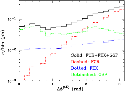
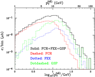
kinematic configurations which are almost , namely and ; elsewhere, FEX and GSP contributions cannot be neglected. This implies that -physics simulations in standard MC’s are always computing intensive. We performed our GSP runs setting GeV; we found that the fraction of events with at least a pair is about 3.7; when the cuts of eq. (86) are applied, this fraction is reduced to 1.6. The dot-dashed histograms in fig. 14 contain only 1900 events, obtained by generating 1.2 GSP events with HERWIG. Although techniques are known to increase the efficiency, and the figures quoted above depend on the particular MC used, it is at present unknown how to generate GSP events with high efficiency.
8.2 -production issues in MC@NLO
In standard shower Monte Carlo programs, the bottom flavour is included in the evolution of the initial-state and final-state showers, consistently with the fact that FEX and GSP processes need also to be considered. On the other hand, as discussed in sect. 3.1 the implementation of MC@NLO is based on FCR processes only. Thus, if we implemented bottom production in exactly the same way as we did with top, we would have to switch off the bottom flavour in all places where it appears in the shower Monte Carlo. This would be particularly problematic for the initial-state shower. Since we normally use five-flavour parton densities, switching off the bottom flavour in backward evolution may lead to inconsistencies.
This problem is not peculiar to MC@NLO implementation. The original NLO calculation of heavy flavour production was carried out in the decoupling scheme of ref. [12], and thus should be used in conjunction with a 4-flavour coupling constant and 4-flavour parton densities. In practice, five-flavour parton densities were always used, since, as pointed out in eq. (3.11) of ref. [13], this is correct (up to a numerically small effect in the gluon parton density) as long as one neglects parton densities with incoming heavy quarks.
In ref. [6], the exact prescription for a change of scheme in the heavy flavour production formulae (in order to go from the decoupling scheme of ref. [12] to the full scheme with 5 flavours) was given. It is summarized as follows:
-
•
Use five-flavour parton densities and strong coupling constant.
-
•
Ignore the and flavours in the parton densities.
-
•
Add a term (where is the renormalization scale) to the channel cross section.
-
•
Add a term (where is the factorization scale) to the channel cross section.
This change of scheme was implemented in the MC@NLO code. The corrections in the last two items above, although necessary to maintain formal correctness at the NLO level, have very small numerical impact. The implementation of the MC@NLO for bottom is then identical to that for top, except for the corrections listed above.
Unlike the case of top production, typical studies of production at hadron colliders are carried out in a relatively large transverse momentum regime, where the bottom flavour behaves in part as a light flavour, and the resummation to all orders of terms may therefore be necessary in order to obtain sensible predictions. In perturbation theory, and for single-inclusive observables, such a resummation is carried out to NLL accuracy by considering all and partonic processes (i.e., including those with one or no in the final state), and convoluting them with NLL perturbative fragmentation functions [14], which describe the evolution of a light parton or a quark into a quark. The resummed formulae can be consistently combined [6] with the exact formulae, in order to obtain reliable predictions for any value.
This procedure has not been extended yet to more exclusive observables. MC@NLO would seem a natural way to achieve this goal, at least at the leading logarithmic accuracy; this would imply implementing, besides the exact FCR formulae, also the ones for light-parton scatterings. The role of the perturbative fragmentation functions would then be played by the showers. The presence of light-parton processes would be taken into proper account in the definition of the MC subtraction terms, in order to avoid double counting. Although this task is not totally out of reach, it is very difficult to achieve it in practice, since it would lead to a great increase in complexity in comparison to the top case.
In the present work we shall restrict ourselves to implementing bottom production with the same accuracy as standard NLO calculations, using the five-flavour strong coupling constant and parton densities in the scheme described above. This allows us to include some leading-log effects (i.e., terms like ), but not all of them. More precisely, single-log terms (of order ) are included exactly in our calculation. The terms of order that are included for any are those that result from multiple final-state radiation from the heavy quark lines, one example of which is illustrated in fig. 15.

Observe that, although the hardest emission is exactly described at the NLO level, subsequent gluon emissions have only a leading-log accuracy, since going to next-to-leading log accuracy would require the implementation of emission kernels (i.e., of showers) at comparable accuracy.
There are also other effects of order that are automatically included in our MC@NLO implementation, which are due to branchings that involve quarks. One such contribution arises when, by backward evolution, a gluon fusion FCR process is connected to a quark line via the initial-state shower. A second type of contribution arises when a final-state gluon, emerging from a FCR hard process, splits into a pair. This splitting process, together with the associated virtual process, gives rise to the correction to the running of due to the bottom flavour. The consistency between the shower evolution including quarks, and the NLO FCR cross sections, is in fact what dictates the use of the five-flavour scheme for and for the parton densities.
However, it is clearly impossible to include all effects of order starting from FCR processes, even with a five-flavour scheme. Most noticeably, the GSP and FEX contributions depicted in fig. 1 are not included in MC@NLO.
In the case of final states containing two or more heavy flavour pairs, the level of precision of the MC@NLO treatment is unclear because one of the pairs (the one produced at the primary NLO vertex) is described differently from those produced by parton showering, as illustrated in fig. 16. As a consequence, the weight factors in the prediction of the bottom pair multiplicity, for example, may not be correct. We postpone discussion of this point to a later date, since from a practical viewpoint multiple pair production is a rare phenomenon (0.1% of single-pair production) which has a negligible effect on the plots shown here.
8.3 Pair correlations
In this section, we present predictions for pair observables. We start by considering the transverse momentum of the pair, . The MC@NLO (solid) and NLO (dotted) results are shown in fig. 17; in the left panel no cuts have been applied, whereas the right panel includes the effect of the cuts given in eq. (86). Regardless of the presence of the cuts,
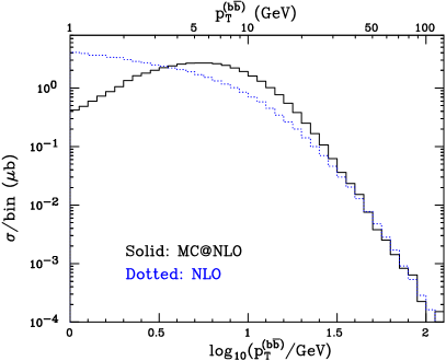
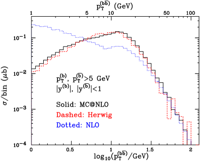
the two plots display the same pattern as the analogous plots for top production (figs. 8 and 11): the NLO distributions diverge for , whereas MC@NLO results have a regular behaviour. On the other hand, in the large- region, dominated by hard-parton emission, MC@NLO and NLO coincide in shape and normalization.
When the cuts of eq. (86) are applied, we can also consider the HERWIG result (dashed histogram), which has been already shown in fig. 14. Unlike the case of top production, here we take HERWIG result with its normalization; a rescaling by the K factor would be more appropriate only if FCR process alone were included. The agreement between MC@NLO and HERWIG is remarkable. In the low- region, we can see that the shape of the MC@NLO result is basically the same as that of HERWIG, analogously to what we have seen in the case of top production. The comparison at large is hampered by the poor statistics of the HERWIG result, since this region receives its main contribution from the GSP process (see fig. 14); however, it appears that MC@NLO and HERWIG agree well. This is not surprising, since a pair produced through the GSP mechanism mainly recoils against a hard gluon, exactly as in the NLO matrix elements which are implemented in MC@NLO. The inability of the MC to produce hard emissions is only evident in the FCR contribution (dashed histogram in fig. 14), which in fact has a much softer behaviour than GSP or MC@NLO.
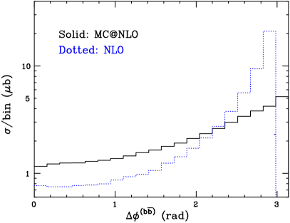
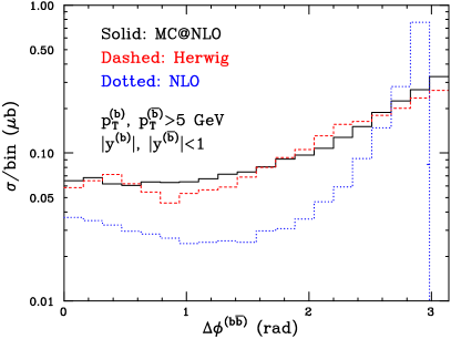
We now turn to the case of the azimuthal distance, . As discussed in sect. 7, this observable receives non-negligible contributions to the tail from both hard emissions and multiple soft or collinear emissions. The presence of large logarithms in the perturbative expansion is manifest at the NLO, since the prediction is strongly peaked towards ; the correct result for the total rate implies that the cross section at is negative. This behaviour is apparent in the dotted histograms in fig. 18. The shapes of the MC@NLO results are similar to the NLO ones in the small- region, but do strongly differ elsewhere. One could perhaps expect that, upon applying the cuts of eq. (86), MC@NLO and NLO would be closer in normalization for ; this doesn’t happen because MC@NLO and NLO have non-negligible differences in the intermediate- region, which dominates the cross section when the cuts of eq. (86) are applied. This fact is not accidental, and will be discussed in sect. 8.4.
As in the case of the transverse momentum of the pair, when the cuts are applied we can also consider the HERWIG prediction (dashed histogram in the right panel of fig. 18). In this case, too, the agreement between MC@NLO and HERWIG is remarkable, and emphasises again the importance of the GSP contribution (see fig. 14). MC@NLO appears to be somewhat more peaked than HERWIG towards .
8.3.1 Impact of initial-state radiation
The results presented above imply that multiple radiation is a crucial effect in production. Lacking an NkLO computation, a typical way of estimating the effects of multiple initial-state emissions on heavy-quark distributions is to supplement an NLO calculation with an intrinsic transverse momentum for the incoming partons (denoted as NLO+-kick hereafter). We stress that this procedure is ill-defined, since there is no way of avoiding double counting. There are however cases in which it is justified from the phenomenological point of view, allowing a much better description of the data than NLO predictions alone (see ref. [11] for a discussion of the implementation of -kick in heavy flavour production, and its implications).
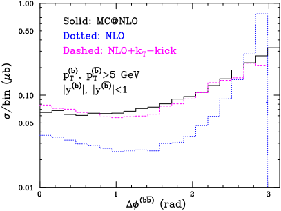
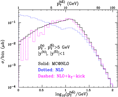
We define our -kick by assuming a gaussian transverse momentum distribution for the incoming partons; we fix the free parameter of this distribution by requiring that the average predicted by NLO+-kick be equal to that obtained from MC@NLO. In this way, the average transverse momentum of the incoming partons turns out to be GeV. With this choice, the NLO+-kick results for the and distributions are seen to agree reasonably with the corresponding MC@NLO results (see fig. 19). This confirms the importance of multiple parton radiation, on top of the possible hard emission present at the NLO level, and shows that the vast majority of the effect is due to emissions from initial-state partons.
The reader is urged not to take NLO+-kick results too seriously, since they are based on a model with little theoretical justification. In fact, an average intrinsic transverse momentum of 4 GeV is too large to be considered a typical non-perturbative effect. On the contrary, in the MC@NLO implementation this effect has a purely perturbative origin, being due to multiple initial-state emissions.
8.4 Single-inclusive observables
We finally turn to the case of single-inclusive -quark distributions. In this section, we shall not consider HERWIG results, because of the findings of sect. 8.1; on the other hand, we do consider the effect of the NLL resummation of large logs , as discussed in sect. 8.2.
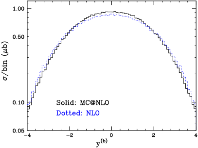
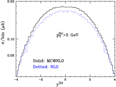
We start with the rapidity of the quark, presented in fig. 20 without and with a transverse momentum cut GeV. Regardless of the presence of this cut, MC@NLO (solid) and NLO (dotted) results agree well. This is to be expected, since for such an observable NLO results are in general reliable.
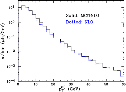
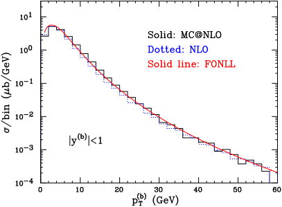
The differences between MC@NLO and NLO results are larger in the case in which a cut is applied. The reason becomes clear if one plots the spectrum, shown in fig. 21. Regardless of the presence of the rapidity cut, the MC@NLO predictions (solid) are above the NLO ones (dotted) in the intermediate- range. When we apply a rapidity cut, we can also consider FONLL predictions [6], based on a formalism that includes not only NLO, terms, but also log-enhanced terms of order (LL) and (NLL). The FONLL result is shown as a solid line in the right panel of fig. 21.
Similarly to MC@NLO, the FONLL result is slightly above the NLO calculation in the region from about 5 to 50 GeV. In the FONLL calculation, this small excess in the intermediate region was attributed to the inclusion in the calculation of higher-order corrections to light parton production (in particular ) followed by gluon fragmentation into a heavy quark (see ref. [6] for details). Neither the NLO, nor the MC@NLO calculations include these corrections. On the other hand, in the MC@NLO implementation the enhancement is very likely due to the transverse momentum boost given to the hard process by the initial state showers. In order to verify this possibility, we use again the NLO+-kick approach used in sect. 8.3.1, with the same parameter setting adopted there. The result is presented in fig. 22.
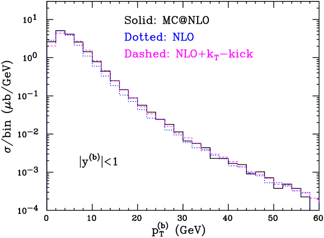
The MC@NLO and NLO+-kick results are again in fair agreement. As in the previous section, we interpret this fact as a hint of the relevance of initial-state multiple emissions in production at the Tevatron. Such effects are not included in FONLL. We thus tentatively speculate that a formalism able to take into account all these effects (i.e. FONLL effects plus multiple soft radiation from the initial-state partons) may result in further enhancement of the intermediate- region with respect to both MC@NLO and FONLL results.
9 Conclusions and future prospects
In this paper we have applied the MC@NLO method to the process of heavy quark production at hadron colliders. The method was developed in ref. [1] and applied there to the process of gauge boson pair production. For heavy quark production, the basic formalism remains the same; it was only necessary to compute the relevant MC subtraction terms and associated colour flows. However, this proved a good deal more complicated than for gauge boson pair production, owing to the presence of coloured objects in the final state even at the Born level, giving rise to different patterns of momentum reshuffling in the MC and more alternative colour flows. In fact, the implementation for heavy quark production demonstrates that MC@NLO can be applied to arbitrarily complicated processes, in terms of kinematics, colour flows and large K factors.
Results were presented on single-particle distributions and correlations at the heavy quark level, with parton showering and hadronization but showing the distributions of the heavy quarks before decay (in the case of top) or hadronization (in the case of bottom), to facilitate comparisons with purely perturbative predictions.
In the case of top quark production, results appear to be fully under perturbative control at Tevatron and LHC energies. The MC@NLO results on single-particle distributions are generally close to those at NLO. A forward-backward asymmetry is seen in the top-quark rapidity distribution at the Tevatron, as expected in NLO but not in LO or in standard MCs which lack exact NLO corrections. In correlations, MC@NLO combines the more correct treatment of hard emissions in NLO with the MC resummation of soft and collinear contributions, giving a smooth distribution of and an enhancement in the distribution when the and are not back-to-back. The effects of hard emissions are naturally more visible at the LHC.
Results on production (presented for the Tevatron only) show more markedly the advantages of the MC@NLO approach compared with conventional MCs. The fact that NLO contributions are included eliminates the need for separate flavour creation (FCR), flavour excitation (FEX) and gluon splitting (GSP) contributions, which are required in standard MCs but are plagued with inefficiencies, ambiguities and cutoff dependences. In fact, we did not attempt to generate single- distributions with the standard HERWIG MC for comparison with MC@NLO and NLO, due to its low efficiency for the GSP contribution. The MC@NLO results, on the other hand, tend to be even more stable than pure NLO, since cancellations between large numbers occur at the matrix-element level, rather than in histograms. They do not depend on cutoffs or on PDFs close to threshold (a source of uncontrolled errors), and thus one can sensibly predict cross sections all the way down to .
MC@NLO predictions for single -quark distributions at the Tevatron are quite similar to those at NLO, with some enhancement at intermediate transverse momenta, which can be interpreted as resulting from Sudakov effects due to multiple initial-state gluon emission.
In the case of correlations at the Tevatron, we could obtain stable HERWIG MC predictions for reasonable values of the cutoff parameter PTMIN, provided the cuts of eq. (86) were imposed. With the resulting mixture of FCR, FEX and GSP contributions, the HERWIG results were then in quite good overall agreement with those of MC@NLO. However, as stressed above, the arbitrariness and inefficiency of the standard MC prescription make the MC@NLO approach vastly preferable from all points of view.
One feature of MC@NLO that might seem unattractive compared with standard MCs is the presence of a fraction (10–20%) of negative weights. As may be seen from the histograms presented here (all generated with unweighted events) this does not cause problems in practice. Most of the negative weights arise from the small- region where the NLO real emission contribution is not resolvable. It may be possible to reduce their contribution further by tuning the subtraction procedure. In spite of the presence of negative weights, MC@NLO is more efficient that standard MCs for production, since it generates the GSP contribution with efficiency 1.
We have not attempted any detailed phenomenological study or comparisons with experimental data in this paper, since our primary objectives were to present the MC@NLO method and compare it with others in the context of heavy quark production. An obvious next step would be to compare with Tevatron data on final-state properties in top and bottom production. In the case of top production, this will require the inclusion of decay correlations due to polarization of the and , which is straightforward in principle but not yet included in the NLO calculation that we have used. In the case of bottom production, careful attention must be paid to the hadronization model used to connect -quark and B-hadron distributions (see app. A.3.2 and ref. [15]).
Other obvious future objectives are the application of MC@NLO to Higgs boson, single vector boson, and jet production. The only extra complication, compared with heavy quark production, arises in the latter case from collinear singularities due to emission from massless final-state partons. The necessary MC subtraction terms can be computed using the kinematics already presented in the present paper. The resulting terms will cancel the additional singularities and should provide more reliable predictions of jet production and fragmentation when combined with a subtraction-method NLO calculation of this process.
Acknowledgements
We thank Rick Field for helpful correspondence. S.F. is grateful for the hospitality of CERN Theory Division during parts of this project.
Appendices
Appendix A Heavy flavour production in HERWIG
We describe here the main features of the HERWIG event generator that are relevant to heavy flavour production. We should distinguish between the standard HERWIG Monte Carlo program and the HERWIG implementation of parton showering and hadronization that forms part of MC@NLO. In the former case the program includes the generation of a hard subprocess as outlined in app. A.1. In the case of MC@NLO, only app. A.2 and A.3 are relevant, since the hard process configurations are read from the input file as explained in sect. 6.2.
A.1 Hard subprocess
The primary heavy quark processes included in the standard HERWIG program are the processes of flavour creation (FCR, eq. (2)), and flavour excitation (FEX, eq. (4) and charge-conjugate processes). However, the hard process configuration is always chosen as if it were FCR, i.e. the kinematics are always chosen for with massless and having the heavy quark mass .
A.1.1 Kinematics
The algorithm for selecting the subprocess kinematics is as follows:
-
1.
Choose the heavy quark transverse mass from a power distribution where PTPOW[4]777Default values (in GeV units) are given in square brackets. with PTMIN[10]PTMAX[].
-
2.
Choose the outgoing parton rapidities uniformly in YJMIN[–8]YJMAX[8] (or in the kinematically allowed region if smaller).
-
3.
Compute the incoming parton light-cone momentum fractions according to
(87) The program also computes at this stage the c.m. scattering angle
(88) -
4.
Compute the kinematic invariants according to
(89)
A.1.2 Dynamics
Having chosen a kinematic configuration, HERWIG calls for PDF evaluations at momentum fractions and hard process scale EMSCA given by
| (90) |
which is also used as the argument of in the calculation of hard process matrix elements.
The program then cycles through all possible FCR and FEX subprocesses, computing the product of relevant PDFs times the on-shell differential cross section evaluated at , times a Jacobean factor. The event weight EVWGT is the sum of all these contributions. In unweighted event generation, if this is greater than the maximum weight times a random number, the configuration is accepted. The program then multiplies EVWGT by another random number, and cycles through the FCR and FEX subprocesses again until the partial sum of contributions exceeds this value. The last subprocess selected is then loaded into the event record as an on-shell process, with the parton momenta reconstructed from the values computed previously.
Note that:
-
1.
Values of are generated only inside the FCR phase space, and so values accessible only in FEX are not explored. In particular the singular FEX point is never generated, even if one sets PTMIN=0.
-
2.
If the process selected is FEX instead of FCR, the reconstructed of the heavy quark is not equal to the originally selected assuming FCR kinematics. An elementary calculation shows that
(91) Thus one always has .
-
3.
In all the above, the masses of light quarks and the effective mass of the gluon are neglected, whereas HERWIG uses these masses (only) in the final step, when it reconstructs the parton momenta from the values of .
A.1.3 Colour structure
HERWIG treats all colour flows as distinct subprocesses. Where the colour flow is ambiguous, it is assigned according to the limit. For example, in the FCR process the colour-averaged matrix element squared is given by eq. (14). In the limit the two colour flows are proportional to and factors in the first bracket, and therefore we assign [16]
| (92) |
with given in eq. (12). In , which we shall call the -flow contribution, gluon 1 is colour-connected to gluon 2 and the heavy quark , while gluon 2 is connected to 1 and . In , the -flow contribution, gluon 1 is colour-connected to 2 and , while 2 is connected to 1 and .
In the other FCR process , the colour connection is uniquely and .
A.2 Parton showers
For a general introduction to the parton shower approximation, see Chapter 5 of ref. [17]. The parton shower in HERWIG [2] is performed using an angular variable [18] and energy fraction . In the parton branching , we have
| (93) |
Thus for massless partons. The evolution scale variable is ; thus the scale set by the above branching is . Colour coherence is simulated by angular ordering, which implies that the initial scales for showering on partons and are and respectively.
The extension of the angular-ordered shower approximation to heavy quark processes is described in ref. [19].
A.2.1 Initial conditions
The initial conditions for parton showering on a given line are determined by the invariant quantity , where is the colour partner of . If is a gluon line, it has two colour partners; one of these is selected at random, with equal probability. The showering on any line is performed in a standard frame, in which the initial energy of is , its direction is along the -axis while that of the colour partner is in the -plane, and the upper limit on the angular evolution variable is . Thus the initial scale for the shower is .
In the FCR processes , when the colour flow is the -flow defined in app. A.1.3 we have for the outgoing heavy quarks, while for each incoming gluon we choose (separately) between and with equal probability. When the colour flow is the -flow, is replaced by . In the process , we have for all the parton showers.
A.2.2 Shower algorithm
In all parton branchings, the leading-order massless splitting functions are used. In timelike (final-state) showering, the allowed region of for the branching is where VQCUT and VGCUT, ([0.32,0.32,0.5]) and [0.75] being the quark and gluon effective masses, and VQCUT[0.48], VGCUT[0.10] minimum virtuality parameters. The argument of is , which is an approximation to the of the emitted gluon888The missing factor of is absorbed into the definition of the QCD scale . – see eq. (49). The corresponding Sudakov form factor is thus
| (94) |
The next value for the evolution variable is selected by solving , where is the current value and is a random number. Branching stops whenever is selected. The minimal value of is .
Spacelike (initial-state) showering is performed backwards, i.e. starting from the hard process. The evolution equation becomes
| (95) |
where is the relevant PDF and is the current value of the energy fraction of the spacelike parton. A compensating factor of multiples the probability distribution in . This “guides” the parton distribution to follow the input PDF. For example, since for , branching to values above 1 is prohibited.
Perturbative branching of the spacelike parton in an initial-state shower stops when a value of QSPAC[2.5]999The default value is relatively high because the input PDF parametrizations may be unreliable (even negative) at lower scales. is selected. However, if the parton is not a valence constituent of the corresponding beam particle, further non-perturbative branching is forced until a valence parton is generated. This is done in order to have a simple model of the beam remnant, composed of the other valence constituents carrying the remainder of the beam momentum.
A.2.3 Azimuthal correlations
After the shower, all the kinematics can be reconstructed from the values of and , except for the azimuthal angles. The distribution of these is isotropic unless dictated otherwise by the logical parameters AZSOFT[.TRUE.] and AZSPIN[.TRUE.]. If AZSOFT is .TRUE., the azimuth of each branching is distributed according to the eikonal formula within the cone defined by the previous branching. In addition, if AZSPIN is also .TRUE., the azimuthal correlation in gluon branching due to gluon polarization is included. Polarization correlations for quarks are neglected, since they vanish due to helicity conservation in the massless limit.
In the processes , where or , there is an azimuthal correlation between the scattering plane and the plane of virtual gluon () emission in initial-state branching, of the form [20] (in the collinear limit)
| (96) |
where is the azimuthal angle between the planes, is the leading-order splitting function,
| (97) |
and
| (98) |
with and .
Since this correlation vanishes in the limit , it is also neglected in HERWIG. However, this means that there is matching between the parton showers and the matrix elements in the collinear limit only after azimuthal averaging of the latter. This poses a problem in MC@NLO implementation, whose solution is discussed in app. B.
A.2.4 Momentum reshuffling
After showering, each external parton line in the hard process has become a jet. The parton momenta have to be replaced by the jet momenta in such a way that energy-momentum is conserved, without seriously affecting the dynamics. This is achieved by the following momentum reshuffling procedure.
Each final-state jet is first rotated from the standard showering frame (see sect. A.2.1) to the direction of the corresponding parton in the hard process c.m. frame, with a rotation about the jet axis to give the correct correlation with the direction of the colour partner. The magnitudes of the jet three-momenta in the hard process c.m. frame are computed as follows. Suppose initially that each jet were given a three-momentum equal to that of the parton it replaces. Since the jet masses are not equal to the parton masses, this would violate energy-momentum conservation. However, energy-momentum conservation can be restored by rescaling the outgoing parton three-momenta in the hard process c.m. frame by a common overall factor, to obtain the jet three-momenta in that frame. Once this factor has been computed, each jet is boosted along its axis to the required three-momentum. Note that the overall four-momentum of the hard process is not changed by this procedure.
In the case of initial-state jets, the partons connected to the incoming beam particles are aligned with the beam directions (smeared by some intrinsic if that is requested through the input parameter PTRMS[0]). Each of the two initial-state jets is then boosted longitudinally (i.e. along the beam directions) until the (now off-shell) momenta of the partons entering the hard process are consistent with the original kinematics. This is not a unique procedure, since not all kinematic variables can be restored to the values they had before showering. There are at present two options, controlled by the logical parameter PRESPL[.TRUE.]:
-
•
If PRESPL is .TRUE., then the c.m. energy and longitudinal momentum of the hard process are preserved (“-scheme”);
-
•
If PRESPL is .FALSE., then the c.m. energy and rapidity of the hard process are preserved (“-scheme”).
Finally the transverse momenta of the initial-state partons entering the hard process are combined to give the transverse momentum of the hard process, and all the final-state jets are boosted transversely, by the amount required for transverse momentum conservation.
In the previous HERWIG version (6.4) the longitudinal and transverse boosts were combined into a single boost in the direction of the new hard process momentum. However, this makes the matching of MC and NLO very complicated. Therefore the two boosts are performed separately in version 6.5. The difference between the two procedures corresponds to a rotation in the hard process c.m. frame (Thomas precession).
One can argue as follows that the effects of momentum reshuffling are beyond the next-to-leading order: to give at least one jet a mass requires one power of , and the average mass-squared is of order . Thus the fractional change in observables due to momentum reshuffling is expected to be of relative order .
A.3 Hadronization
A.3.1 Cluster formation
After the perturbative parton showering and momentum reshuffling, all outgoing gluons are split non-perturbatively, into light quark-antiquark or diquark-antidiquark pairs (the default option is to disallow diquark splitting). At this point, each jet consists of a set of outgoing quarks and antiquarks (also possibly some diquarks and antidiquarks) and, in the case of spacelike jets, a single incoming valence quark or antiquark. The latter is replaced by an outgoing spectator carrying the opposite colour and the residual flavour and momentum of the corresponding beam hadron.
In the limit of a large number of colours, each final-state colour line can now be followed from a quark/anti-diquark to an antiquark/diquark with which it can form a colour-singlet cluster. By virtue of the preconfinement property of the shower [21], these clusters have a distribution of mass and spatial size that peaks at low values, falls rapidly for large cluster masses and sizes, and is asymptotically independent of the hard subprocess type and scale.
The clusters thus formed are fragmented into hadrons. If a cluster is too light to decay into two hadrons, it is taken to represent the lightest single hadron of its flavour. Its mass is shifted to the appropriate value by an exchange of 4-momentum with a neighbouring cluster in the jet. Similarly, any diquark-antidiquark clusters with masses below threshold for decay into a baryon-antibaryon pair are shifted to the threshold via a transfer of 4-momentum to a neighbouring cluster.
Those clusters massive enough to decay into two hadrons, but below a fission threshold to be specified below, decay isotropically101010Except for those containing a ‘perturbative’ quark when CLDIR=1 – see below. into pairs of hadrons selected in the following way. A flavour is chosen at random from among , , , the six corresponding diquark flavour combinations, and . For a cluster of flavour , this specifies the flavours and of the decay products, which are then selected at random from tables of hadrons of those flavours. The selected choice of decay products is accepted in proportion to the density of states (phase space times spin degeneracy) for that channel. Otherwise, is rejected and the procedure is repeated.
A fraction of clusters have masses too high for isotropic two-body decay to be a reasonable ansatz, even though the cluster mass spectrum falls rapidly (faster than any power) at high masses. These clusters are fragmented using an iterative fission model until the masses of the fission products fall below the fission threshold. In the fission model the produced flavour is limited to , or and the product clusters and move in the directions of the original constituents and in their c.m. frame. Thus the fission mechanism is not unlike string fragmentation [22].
In HERWIG there are three main fission parameters, CLMAX[3.35], CLPOW[2] and PSPLT[1]. The maximum cluster mass parameter CLMAX and CLPOW specify the fission threshold according to the formula
| (99) |
where and are the quark mass (RMASS) parameters for flavours and . The parameter PSPLT specifies the mass spectrum of the produced clusters, which is taken to be within the allowed phase space. Provided the parameter CLMAX is not chosen too small, the gross features of events are insensitive to the details of the fission model, since only a small fraction of clusters undergo fission. However, the production rates of high- or heavy particles (especially baryons) are affected, because they are sensitive to the tail of the cluster mass distribution. Reducing CLPOW increases the yield of heavier clusters (and hence of baryons) for heavy quarks, without affecting light quarks much. For example, the default value gives no -baryons (for the default value of CLMAX) whereas CLPOW=1.0 makes the ratio of -baryons to -hadrons about 1/4.
There is also a switch CLDIR[1] for cluster decays. For the default value, a cluster that contains a ‘perturbative’ quark, i.e. one coming from the perturbative stage of the event (the hard process or perturbative gluon splitting) ‘remembers’ its direction. Thus when the cluster decays, the hadron carrying its flavour continues in the same direction (in the cluster c.m. frame) as the quark. This considerably hardens the spectrum of heavy hadrons, particularly of - and -flavoured hadrons. CLDIR=0 turns off this option, treating clusters containing quarks of perturbative and non-perturbative origin equivalently.
In the CLDIR=1 option, the parameter CLSMR[0] allows for a Gaussian smearing of the direction of the perturbative quark momentum. The smearing is actually exponential in with mean value CLSMR. Thus increasing CLSMR decorrelates the cluster decay from the initial quark direction.
A.3.2 -quark hadronization
The process of -quark hadronization requires special treatment and the results obtained using HERWIG are still not fully satisfactory. Generally speaking, it is difficult to obtain a sufficiently hard B-hadron spectrum and the observed -meson/-baryon ratio. These depend not only on the perturbative subprocess and parton shower but also on non-perturbative issues such as the fraction of -flavoured clusters that become a single B meson, the fractions that decay into a B meson and another meson, or into a -baryon and an antibaryon, and the fraction that are split into more clusters. Thus the properties of -jets depend on the parameters RMASS(5), CLMAX, CLPOW and PSPLT in a rather complicated way. In practice these parameters are tuned to global final-state properties and one needs extra parameters to describe -jets.
A parameter B1LIM[0] has therefore been introduced to allow clusters somewhat above the B threshold mass to form a single B meson if
| (100) |
The probability of such single-meson clustering is assumed to decrease linearly for . This has the effect of hardening the B spectrum if B1LIM is increased from the default value.
In addition, in HERWIG version 6, the parameters PSPLT, CLDIR and CLSMR have been converted into two-dimensional arrays, with the first element controlling clusters that do not contain a -quark and the second those that do. Thus tuning of -fragmentation can now be performed separately from other flavours, by setting CLDIR(2)=1 and varying PSPLT(2) and CLSMR(2). By reducing the value of PSPLT(2), further hardening of the B-hadron spectrum can be achieved.

Figure 23 shows the fragmentation function in decay, i.e. the distribution of the energy fraction in collisions, where is the energy of a weakly-decaying -flavoured hadron in the rest frame. The HERWIG predictions for different values of some of the parameters discussed above are compared with the data of the SLD Collaboration [23]. For the MC@NLO predictions in sect. 8, parameters were left at their default values except for PSPLT(2)=0.5, corresponding to the long-dashed curve. However, as explained in sect. 8, all the results presented there are at the -quark level, and are therefore insensitive to the -hadronization parameters.
Appendix B MC subtraction terms
In this section, we derive the MC subtraction terms needed in order to define MC@NLO, eq. (1). We follow , sect. A.5. In the present case, the term in the expansion of the result of HERWIG is given in eq. (60), which we report again here
| (101) |
This equation is identical to eq. (I.A.58), except for the fact that more emitting legs and colour structures have been considered.
We start from the case of initial-state radiation, considering emission from leg 1 for definiteness. We can rewrite the relevant part of eq. (I.A.58)) as follows:
| (102) | |||||
where we have explicitly indicated the integration over the azimuthal angle of the branching parton (which is trivial here but will not be so in the following). We have used the findings of sects. 4.1.2 and 4.2.2. The momentum fractions of the partons entering the hard process are , and , given in eqs. (39) and (41) in the - and -scheme respectively (see sect. A.2.4). The -channel invariant is , given in eq. (4.1.2). The set fully specifies the momenta of the hard process in the lab frame. In fact, the -channel invariant is
| (103) |
where is given in eq. (4.1.2), and the last equality holds thanks to eq. (37). With , , and one gets immediately the momenta in the hard c.m. frame:111111In order to simplify the notation, the momenta have been rotated in the transverse plane along the direction corresponding to .
| (104) |
where from eq. (8)
| (105) |
Finally, the momenta in eq. (104) are boosted to the lab frame with
| (106) |
In eq. (102), is the Born matrix element squared, summed over spin and colour degrees of freedom (the average factor for initial-state ones is understood), times the flux factor, times a factor which depends on the partonic process and the colour flow. When this factor is one; when , it is one for , whereas for we have , with given in eq. (92). depends on and only through their product; however, we use the notation of eq. (102) order to remember the boost of eq. (106).
We now perform some changes of integration variables in eq. (102). We replace with , the fractional parton momenta of the process. We also replace with . Here, we do not need to define these variables precisely; they are used in order to eliminate the dependence upon the index in the integration measure, and will be related to the three-body phase-space variables in the following. Finally, we use the fact that, in the c.m. frame of the hard process, the two-body phase space can be written as follows
| (107) |
where the function is given in eq. (9). We thus get
| (108) |
The factor contains the dependence upon parton densities
| (109) |
The actual form of the Jacobean that appears in this equation depends on the momentum reshuffling scheme (see app. A.2.4). By explicit computation, using eqs. (39) and (59) we find, in the -scheme,
| (110) |
In the -scheme, we use eqs. (41) and (59) to obtain
| (111) |
The factor collects the terms related to parton branching
| (112) |
In contrast to the case of (see eq. (I.A.72)) the Jacobean has in general a non-trivial dependence upon the azimuthal angles; this is so in the cases , and it is due to the complicated dependence of the HERWIG scale upon the phase-space variables. Finally, the factor contains the full information on the hard process, and phase-space factors
| (113) |
We now turn to the case of final-state branching, considering emission from the heavy quark. The analogue of eq. (102) reads
| (114) | |||||
Here, the results of sects. 4.1.1 and 4.2.1 have to be used. The momentum fractions of the incoming partons are not affected by final-state branching, and eq. (26) holds; therefore
| (115) |
The -channel invariant is given in eq. (4.1.1). The momenta of the hard process are given in eq. (104) in the parton c.m. frame, with , , and computed as in eqs. (105) after the formal replacements . These momenta are subsequently boosted to the lab frame by means of
| (116) |
Performing changes of variables analogue to those in eq. (102), we get the analogue of eq. (108)
| (117) |
where now121212For final-state emission the Jacobean factor for the Bjorken ’s is trivial, see eq. (26).
| (118) | |||||
| (119) | |||||
| (120) |
Equation (108) and (117) are closely related to the MC subtraction terms needed for the definition of MC@NLO. We use eq. (I.A.61)
| (121) |
In order to proceed, we introduce an explicit parametrization for the three-body phase space. We use (see eq. (I.A.10))
| (122) |
where is the scattering angle of in the c.m. frame. The variables , and refer to the emitted parton in the parton c.m. frame of the process: is the energy in units , and and are the cosine of the polar angle and the azimuthal angle respectively; and can be expressed in terms of invariants as shown in eq. (59). The ranges of the angular variables are , . The parametrization of eq. (122) is identical to that of eq. (2.12) of ref. [3], provided that a (physically irrelevant) rotation of is performed there, in the transverse plane in the c.m. frame. The momenta parametrizations of eqs. (2.8) of that paper can thus be used here. We use eq. (122) to rewrite eqs. (108) and (117) as follows
| (123) | |||||
| (124) |
where we have chosen and to coincide with , and131313Here and in what follows we have some abuse of notation, since we denote by the same symbols , , and quantities which possibly differ by multiplicative factors from those previously introduced.
| (125) | |||||
| (126) | |||||
| (127) | |||||
| (128) | |||||
| (129) | |||||
| (130) |
Here, we have used and . The quantities and depend on , , and the invariants; thus, the Jacobean in eq. (125) must be computed at fixed . Furthermore, the Jacobeans in eq. (126) and (129) have to be computed at fixed and respectively.
The MC subtraction terms appear twice in the definition of MC@NLO, eq. (1), since they contribute to the weights of and events. These weights are treated as ordinary MC weights in the MC evolutions, whose generating functionals are and respectively. Implicit in these generating functionals is also the dependence upon the initial conditions for the showers, i.e. the momenta of the and processes. As the integral in eq. (1) requires, these momenta need to be specified for each point in the integration range . This is straightforward in the case of events, after a definite parametrization is chosen for the angles and , which allows the computation of the Jacobeans that appear in eqs. (127) and (130).
The situation is more involved in the case of events. Since here the initial condition for the shower is a process, a mapping of the three-body phase space onto the two-body one is necessary. This map is provided by the MC, which relates the momenta of the partons entering the hard process to those of the partons emerging from the shower. In the case of a single branching, this map has been denoted by in sect. 2. In this section, we have given explicit implementations of : in the case of initial-state emission, one uses eqs. (104)–(106), where the invariants are expressed in terms of the ones as explained in sect. 4.1.2. For final-state emission, analogous relations hold (see the discussion after eq. (115)). These maps also provide us with the definitions of the scattering angles and in terms of the three-body phase-space variables. In fact, the -channel invariant is always given by the function (see eq. (10))
| (131) |
and being the -channel invariant and scattering angle in the hard c.m. frame respectively. Thus, taking into account eq. (27), and the fact that , we have
| (132) | |||
| (133) |
which can be solved for and using eqs. (4.1.2) and (4.1.1) respectively.
However, eqs. (132) and (133) manifestly define two different maps and , whereas eq. (1) requires . In fact, if , for a given three-body configuration one would get two two-body configurations generated by and , and the choice of which one to use in as initial condition for the shower would result in an ambiguity in MC@NLO. Besides, the complicated functional relations implicit in eq. (132) and (133) would make the task of the implementation of event projection in the NLO cross section a difficult one.
A solution for the first problem mentioned above is to treat initial- and final-state emissions independently in MC@NLO. The NLO cross section must also be written accordingly, since MC subtraction terms act as local counterterms. This can be achieved for example using the technique of ref. [20], which basically amounts to partitioning the phase space into regions dominated by initial- or final-state emissions.141414Ref. [20] is based on the subtraction method, so no approximation is involved in this phase-space partition. In terms of numerical accuracy and unweighting efficiency this may be the best strategy in those cases in which final-state collinear emissions are singular at the level of short-distance cross sections, such as in jet physics. However, it would still leave us with the problem of an easy implementation of event projection.
We argue that, regardless of the presence of final-state singularities in real matrix elements, the simplest possible definitions of the maps and should be adopted. We now show how this can be achieved; as a by product, we also show that, in the present case, initial- and final-state emissions can indeed be treated simultaneously.
We start by observing that momentum reshuffling is an effect beyond NLO (see sect. A.2.4). It follows that two kinematic configurations are equivalent at the NLO if they coincide in the limit in which the off-shell parton (i.e., the parton which has branched) has its on-shellness restored. This is a consequence of the fact that the branching procedure is exact only for zero-angle emission. Thus, for a given configuration we can take its zero-angle-emission limit, and extract from there the momenta we seek. This is most easily done in the partonic c.m. frame, where eq. (104) holds; eqs. (105) are then used to obtain , , and , with the invariants expressed in terms of the zero-angle limits of the invariants. The limits can be computed by choosing any parametrization for the three-body phase space; in the following, we shall use eq. (122), exploiting the explicit formulae of ref. [3].
For initial-state emission (say, from parton 1), from eq. (4.1.2) we get, in the zero-angle-emission limit
| (134) |
Replacing with in eq. (132), and solving for , we get
| (135) |
This is what we expect, since for strictly collinear initial-state emission, the parton c.m. frame (where is defined) and the c.m. frame (where is defined) coincide.
For final-state emission from the quark leg, from eq. (4.1.1) we get
| (136) |
where
| (137) |
Note that
| (138) |
which is what one expects on physical grounds, since is the soft limit in the parametrization of eq. (122), and it is only in this limit that the parton c.m. frame and the c.m. frame coincide in the case of final-state emission.
We can now use eqs. (135) and (137) in eqs. (127) and (130) respectively. This fully defines the MC subtraction terms, at least in the case of events, where the initial condition for the MC shower is given by the configuration, as specified by the integration variables . However, we still have the problem that . To see this explicitly, we write the momenta that we obtain with the zero-angle-emission prescription:
for initial-state emission
| (139) |
for final-state emission
| (140) |
with given in eq. (137). The momenta in eq. (139) are then boosted to the lab frame using eq. (106), those in eq. (140) using eq. (116). We now observe that the momenta in eq. (139) can be obtained with the parametrization of eq. (122) by imposing the soft limit , but freezing the c.m. energy to the value . Furthermore, as described in sect. 4.1.1, for final-state emission the reshuffling does not change the direction of the outgoing heavy quark in the partonic c.m. frame; thanks to eq. (138), a practical way of computing it is to consider the soft-emission limit in the parametrization of eq. (122). Thus, in the soft limit the scattering angles in the parton c.m. frames coincide for initial- and final-state emission. Unfortunately, the momenta do not coincide, because of the different -channel invariants and boosts to the lab frame. However, we can force them to coincide with a simple formal manipulation, similar to what is done for event projection. We can use the identity in eq. (139), and in eq. (140). Next, we formally replace with and with in eq. (124) (which is allowed, these variables being just integration variables there), and then we change integration variables back to and . Eqs. (128) and (130) become
| (141) | |||||
| (142) |
In may appear counterintuitive to have a dependence on and in these equations. However, it must be clear that this has nothing to do with initial-state emission. Simply, the freedom of changing integration variables allowed us to scale the partonic c.m. energy in eq. (124) by a factor of . Thus, eq. (139) now holds for final-state emission as well. Furthermore, the boost to the lab frame is now performed with eq. (106) rather than with eq. (116). This is precisely what we wanted to achieve, since a unique has now been defined. For a given choice of , one reconstructs the momenta in the hard c.m. frame by taking the soft limit with the -channel invariant fixed to , and then boosts to the lab frame using eq. (106).
We stress that, in the case of final-state emissions, we define the MC subtraction terms using eqs. (128)–(130) for events, and eqs. (141)–(142) for events. In principle, we should therefore introduce the notations and , but we prefer to avoid it, since it has been shown that the difference between the two amounts to a change in the integration variables.
The zero-angle procedure implies the possibility of several definitions of the MC subtraction terms, which differ beyond NLO. For example, one could use the invariants obtained in the zero-angle-emission limit, eqs. (134) and (136), in the computation of the hard matrix elements, for both and event, or only for events. We prefer not to consider the latter option, which results in a total rate computed by the MC@NLO different from the NLO one. The former choice has indeed been implemented; the results have been found to be identical to those obtained with our default choice in the case of top production. When bottom production is considered, very small differences are visible in the tails of those distributions which are effectively of leading-order accuracy in the fixed-order computation of ref. [3], such as the transverse momentum of the pair or . However, these differences never exceed a few percent, and are much smaller than the uncertainties of the fixed-order results due to scale variation. This confirms that reshuffling effects are beyond the accuracy of MC@NLO.
As pointed out in , sect. A.5, the MC subtraction terms given in eqs. (123) and (124) cannot act as local counterterms for real emission matrix elements, since the angular distribution of a soft gluon emitted by the MC does not agree with the corresponding perturbative result. However, it has been argued in that this effect must be irrelevant in the definition of observables, at least for infrared-safe ones. Thus, in the MC subtraction terms were defined by smoothly matching what is obtained from the perturbative expansion of the MC result with the leading singular behaviour of the real matrix elements in the soft limit. The matching has been defined through a parameter-dependent damping function, eq. (I.A.86). The physical observables were found to be independent of the parameters used to define the damping function, thus practically confirming that infrared-safe observables are insensitive to the angular distribution of soft-gluon emission.
Here, we shall follow the same strategy. Since the soft singularity structure is more complicated than in the case of gauge-boson pair production, and in particular cannot be associated with the soft divergence of an Altarelli-Parisi splitting function, we generalize eq. (I.A.83) and eq. (I.A.84) as follows:
| (143) | |||||
where , and denote the leading singular behaviour of the real matrix element in the soft, collinear, and soft-collinear limits respectively. The functional form of the damping functions and is the same, and is given in eq. (I.A.86) (with ); the subscript is to remind us that the parameters these functions contain can be varied independently. The function smoothly approaches zero in the soft limit
| (144) |
and the function smoothly approaches zero in the initial-state collinear limits
| (145) |
Note that the function would not be necessary away from the soft limit, if azimuthal correlations (see app. A.2.3) were either absent or properly described by the MC. As in , no evidence has been found of a dependence of the physical results upon the parameters entering the damping functions.
In summary, eq. (143) is our final formula for MC subtraction terms. The quantities are defined in eqs. (123) and (124) for initial- and final-state emissions respectively. , , and appearing there are given in eqs. (125)–(127) for initial-state emissions. For final-state emissions, we use eqs. (128)–(130) for events, and eqs. (129), (141), (142) for events.
Appendix C Colour flow codes
We list in tables 3 and 4 the codes IC used in MC@NLO to transmit colour flow information to the HERWIG event generator. The convention is that and represent the colour and anticolour of parton . If is a quark (antiquark) then its anticolour (colour) is zero. Thus for example when , corresponding to (see table 4), we have , , , meaning that and are colour-connected, and are anticolour-connected, and the anticolour of is connected to the colour of . In accordance with the Les Houches convention, the non-zero colour labels entered into the event common block HEPEUP are actually and .
| IC | |||||
|---|---|---|---|---|---|
| 1 | 10 | 02 | 10 | 02 | |
| 2 | 01 | 20 | 20 | 01 | |
| 3 | 12 | 23 | 10 | 03 | |
| 4 | 12 | 31 | 30 | 02 |
| IC | ||||||
|---|---|---|---|---|---|---|
| 1 | 10 | 02 | 13 | 30 | 02 | |
| 2 | 10 | 02 | 32 | 10 | 03 | |
| 3 | 10 | 21 | 30 | 20 | 03 | |
| 4 | 10 | 23 | 20 | 10 | 03 | |
| 5 | 01 | 20 | 23 | 30 | 01 | |
| 6 | 01 | 20 | 31 | 20 | 03 | |
| 7 | 01 | 23 | 03 | 20 | 01 | |
| 8 | 01 | 12 | 03 | 30 | 02 | |
| 9 | 12 | 20 | 30 | 10 | 03 | |
| 10 | 12 | 30 | 10 | 30 | 02 | |
| 11 | 12 | 03 | 02 | 10 | 03 | |
| 12 | 12 | 01 | 03 | 30 | 02 | |
| 13 | 12 | 23 | 14 | 40 | 03 | |
| 14 | 12 | 34 | 32 | 10 | 04 | |
| 15 | 12 | 23 | 43 | 10 | 04 | |
| 16 | 12 | 31 | 34 | 40 | 02 | |
| 17 | 12 | 34 | 14 | 30 | 02 | |
| 18 | 12 | 31 | 42 | 30 | 04 |
Appendix D subtraction
In I, an NLO subtraction scheme was introduced, called subtraction, which allows one to reduce the number of negative-weight events occurring in MC@NLO, compared to that resulting from the implementation of the “standard” subtraction formulae of ref. [24], in which the computation of W+W- cross sections to NLO accuracy was originally performed. The subtraction is essentially defined by the requirement that the subtraction terms be non-zero only in the region
| (146) |
being the transverse momentum of the real parton emitted at the NLO. In terms of the variables and (see eqs. (144) and (145) for their boost-invariant definitions, and eq. (122) for an explicit phase-space parametrization which uses them), eq. (146) becomes
| (147) |
As pointed out in I, eq. (147) is not specific to vector boson pair production, and can be applied to any NLO cross section. However, the formulae for the partonic cross sections derived in app. A.3 of I need to be generalized. That is the aim of this section. Although we shall closely follow the notation of ref. [3], it will be clear that our results are relevant to any hard production process of a heavy (or hard) system, for which the matrix elements have all possible soft and collinear divergencies, except those due to final-state collinear emissions.
We start by observing that eq. (147) implies that there is a minimum value of , for fixed , equal to
| (148) |
where is the minimum value of allowed by kinematics (for heavy flavour production, ). We then write the analogue of eq. (3.5) of ref. [3] in a more general form151515Consistently with app. B, and unlike the convention of ref. [3], we have here .
| (149) |
where is the -dimensional () reduced phase space for the production of the heavy system with a squared invariant mass equal to . In we also incorporate further normalization factors, that reduce to 1 in 4 dimensions. Thus, the phase space of the heavy system plus the light parton is
| (150) |
In the present context, the precise -dimensional form of is irrelevant. The only thing we need to know is that in 4 dimensions it is equal to the phase space of the reduced system. Thus, in the case of heavy flavour production
| (151) |
which coincides with eq. (107) for . Using this equation in eq. (150), we get in 4 dimensions, with given in eq. (122). In eq. (149), we have also defined as
| (152) |
where is the invariant spin-averaged squared amplitude divided by the flux factor. Its dependence upon the kinematic variables of the reduced system ( in the case of heavy flavour production) is not explicitly shown.
Following the reasoning of ref. [3], we now use the expansion
| (153) |
with (notice that here depends on , which is not the case in ref. [3]). This yields
| (154) | |||||
where
| (155) |
with . We can now expand
| (156) |
where we define
| (157) |
This quantity has the same formal meaning as in ref. [3]; unlike , however, it does depend on . Using eq. (156) in eq. (154) we get
| (158) |
where
| (159) | |||||
and
| (160) |
Notice that prescriptions, rather than prescriptions, appear in eq. (159), since for . Furthermore, the expression in eq. (159) does not need a regularization prescription, since as also .
To see precisely the structure of the generated counterterms in , let us expand the expression
| (161) |
according to the definition of the distributions. Here represents symbolically some function of the final-state kinematics, regular for and . We get
| (162) | |||
where in the middle (last) expression we have used the fact that when ( when ). Using the relation
| (163) |
we can rewrite the above expression as
| (164) |
The last term is finite by itself, since
| (165) |
It is a soft term, which we can rewrite by explicitly computing the integral over
| (166) |
For consistency with I, we include this term in , which is then modified with the replacement
| (167) |
We now present the corrections to be added to the soft and collinear terms in order to go from the standard subtraction scheme of ref. [3] (computed with and ) to the -subtraction scheme. In the soft term, the correction is given by
| (168) |
We find
| (169) | |||||
Since the function implies , we only need to expand the square bracket to order , thus getting
| (170) |
So, our final formula for the correction is
| (171) |
with (see eq. (I.A.27))
| (172) |
The soft limit is non-zero only if the radiated parton is a gluon. It is given in general by a sum over eikonal factors
| (173) |
where are the external momenta of the reduced process, is the momentum of the soft gluon, and are functions of the momenta of the reduced process. Expressions for in the case of heavy quark production can be easily obtained (after correcting a couple of misprints161616 in the last line of eq. (A.12) should read , and the in the last line of eq. (A.21) should read ) from Appendix A of ref. [3]. Terms arising from the eikonal factor associated with initial-state soft emissions can be integrated analytically over and in eq. (171). For the other terms, only the azimuthal integration can be easily computed analytically. The integration is performed numerically.
The collinear correction is
| (174) |
Finally, for the finite part of the real cross section an equation identical to eq. (I.A.26) holds:171717In eq. (I.A.26) a different notation is used, which leads to an error if one forgets to freeze when applying the prescriptions, as required in eqs. (I.A.21)–(I.A.23).
| (175) |
where the -distribution prescription is defined by
| (176) | |||
We now discuss the relation of the above results with the results of I. The collinear correction is equivalent to the term
of eq. (I.A.25). In the case of the soft correction, only the terms corresponding to are non-zero in eq. (173); these can be integrated analytically, yielding the term in eq. (I.A.24).
In the case of heavy flavour production, we find that subtraction reduces only marginally (1%–2%) the number of negative weights with respect to standard subtraction. In fact, due to the simultaneous presence of several colour flows which induce different dead zones (see figs. 2 and 3), the subtraction region of eq. (147) never matches closely the region in which HERWIG radiation is allowed. Nevertheless, it is still advantageous to use subtraction, since the parameter tuning, necessary to reduce as much as possible the number of negative weights, is easier than in the case of standard subtraction (simply because the latter depends on two parameters rather than one).
References
- [1] S. Frixione and B. R. Webber, “Matching NLO QCD computations and parton shower simulations,” JHEP 0206 (2002) 029 [arXiv:hep-ph/0204244]. See also http://www.hep.phy.cam.ac.uk/theory/webber/MCatNLO/.
- [2] G. Corcella et al., “HERWIG 6: An event generator for hadron emission reactions with interfering gluons (including supersymmetric processes),” JHEP 0101 (2001) 010 [arXiv:hep-ph/0011363].
- [3] M. L. Mangano, P. Nason and G. Ridolfi, “Heavy Quark Correlations In Hadron Collisions At Next-To-Leading Order,” Nucl. Phys. B 373 (1992) 295.
- [4] E. Norrbin and T. Sjostrand, “Production and hadronization of heavy quarks,” Eur. Phys. J. C 17 (2000) 137 [arXiv:hep-ph/0005110].
- [5] R. D. Field, “The sources of b quarks at the Tevatron and their correlations,” Phys. Rev. D 65 (2002) 094006 [arXiv:hep-ph/0201112].
- [6] M. Cacciari, M. Greco and P. Nason, “The p(T) spectrum in heavy-flavour hadroproduction,” JHEP 9805 (1998) 007 [arXiv:hep-ph/9803400].
- [7] G. Corcella and M. H. Seymour, “Initial state radiation in simulations of vector boson production at hadron colliders,” Nucl. Phys. B 565 (2000) 227 [arXiv:hep-ph/9908388].
- [8] S. Kawabata, “A New version of the multidimensional integration and event generation package BASES/SPRING,” Comput. Phys. Commun. 88 (1995) 309.
- [9] E. Boos et al., “Generic user process interface for event generators,” arXiv:hep-ph/0109068.
- [10] A. D. Martin, R. G. Roberts, W. J. Stirling and R. S. Thorne, “Parton distributions and the LHC: W and Z production,” Eur. Phys. J. C 14 (2000) 133 [arXiv:hep-ph/9907231].
- [11] S. Frixione, M. L. Mangano, P. Nason and G. Ridolfi, “Heavy-quark production,” Adv. Ser. Direct. High Energy Phys. 15 (1998) 609 [arXiv:hep-ph/9702287].
- [12] J. C. Collins, F. Wilczek and A. Zee, “Low-Energy Manifestations Of Heavy Particles: Application To The Neutral Current,” Phys. Rev. D 18 (1978) 242.
- [13] P. Nason, S. Dawson and R. K. Ellis, “The One Particle Inclusive Differential Cross-Section For Heavy Quark Production In Hadronic Collisions,” Nucl. Phys. B 327 (1989) 49 [Erratum-ibid. B 335 (1990) 260].
- [14] B. Mele and P. Nason, “The Fragmentation Function For Heavy Quarks In QCD,” Nucl. Phys. B 361 (1991) 626.
- [15] M. Cacciari and P. Nason, “Is there a significant excess in bottom hadroproduction at the Tevatron?,” Phys. Rev. Lett. 89 (2002) 122003 [arXiv:hep-ph/0204025].
- [16] K. Odagiri, “Color connection structure of (supersymmetric) QCD (2 2) processes,” JHEP 9810 (1998) 006 [arXiv:hep-ph/9806531].
- [17] R. K. Ellis, W. J. Stirling and B. R. Webber, “QCD and Collider Physics,” Cambridge Monogr. Part. Phys. Nucl. Phys. Cosmol. 8 (1996) 1.
- [18] G. Marchesini and B. R. Webber, “Simulation Of QCD Jets Including Soft Gluon Interference,” Nucl. Phys. B 238 (1984) 1.
- [19] G. Marchesini and B. R. Webber, “Simulation Of QCD Coherence In Heavy Quark Production And Decay,” Nucl. Phys. B 330 (1990) 261.
- [20] S. Frixione, Z. Kunszt and A. Signer, “Three-jet cross sections to next-to-leading order,” Nucl. Phys. B 467 (1996) 399 [arXiv:hep-ph/9512328].
- [21] D. Amati and G. Veneziano, “Preconfinement As A Property Of Perturbative QCD,” Phys. Lett. B 83 (1979) 87.
- [22] B. Andersson, G. Gustafson, G. Ingelman and T. Sjostrand, “Parton Fragmentation And String Dynamics,” Phys. Rept. 97 (1983) 31.
- [23] K. Abe et al. [SLD Collaboration], “Measurement of the b-quark fragmentation function in Z0 decays,” Phys. Rev. D 65 (2002) 092006 [Erratum-ibid. D 66 (2002) 079905] [arXiv:hep-ex/0202031].
- [24] S. Frixione, “A Next-to-leading order calculation of the cross-section for the production of W+ W- pairs in hadronic collisions,” Nucl. Phys. B 410 (1993) 280.