TUHEP-TH-03144

Nonsymmetric Gravity and Noncommutative Signals

N. Kersting^a, and Y.L. Ma^a

^a Theoretical Physics Group, Department of Physics Tsinghua University, Beijing P.R.C. 100084

Models in which the space-time metric $g_{\mu\nu}$ is not symmetric, $\it i.e.$ $g_{\mu\nu}\neq g_{\nu\mu}$ may make predictions in scattering experiments, for example in a future $e^{+}e^{-}$ linear collider, similar to those from noncommutative field theory. We compute the differential cross sections for pair annihilation, Bhabha and M$\o$ller scattering and find that both nonsymmetric gravity theory(NGT) and noncommutative field theory predict a similar dependence of the differential cross section on the azimuthal angle in agreement with all known data, however in NGT Lorentz violation need not be as severe. Astrophysical and cosmological tests may prove very useful in distinguishing these two theories.

1 Introduction

If Nature violates isotropy of space or commutivity among coordinate displacements, the basic assumptions at the root of most of physics come into question and it becomes imperative to parametrize this violation, devising tests to put limits on the parameters. Two such parameterizations in this direction involve the theories of noncommuting space coordinates [1] and nonsymmetric gravity [2]. Particle physics experiments at future hadronic or linear colliders may provide good testing grounds for these theories.

In nonsymmetric gravity theory (NGT) the metric of space-time is taken to be nonsymmetric, $\it i.e.$ $g_{\mu\nu}\neq g_{\nu\mu}$. In particular, we may write

$$g_{\mu\nu}=g_{(\mu\nu)}+g_{[\mu\nu]}$$ (1)

decomposing $g$ into its symmetric and antisymmetric pieces. The contravariant tensor $g^{\mu\nu}$ is defined as usual:

$$g^{\mu\nu}g_{\mu\rho}=\delta^{\nu}_{\rho}$$ (2)

One can now go on to define a Lagrangian density as in general relativity, ${\cal L}=\sqrt{-g}R$, where $g\equiv det(g_{\mu\nu})$ and $R$ is the Ricci scalar, and derive field equations for $g_{(\mu\nu)}$ and $g_{[\mu\nu]}$. More details on this reformulation of general relativiy can be found in  [2]. There has been extensive work analyzing the effects of $g_{[\mu\nu]}$ for black hole solutions of the field equations, galaxy dynamics, stellar stability, and other phenomena of cosmological and astrophysical relevance  [3, 4, 5] where $g_{(\mu\nu)}$ and $g_{[\mu\nu]}$ may be of comparable size.

In the context of particle physics however, we may start with the assumption that the curvature of space in the region of interest is small:

$$g_{\mu\nu}\approx\eta_{\mu\nu}+h_{(\mu\nu)}+a_{[\mu\nu]}$$ (3)

where $\eta$ is the usual Minkowski metric and both  $h$ and $a$ satisfy $a_{\mu\nu},h_{\mu\nu}\ll 1~{}\forall~{}\mu,\nu$. We further assume that these fields’ dynamics are negligable in the region of interest and we may treat them as background fields. The effects of the symmetric tensor $h$ on particle physics in this limit has been studied elsewhere (see for example  [6, 7, 8]). We would like to focus our attention here on the effects of the antisymmetric piece $a$.

We therefore take $h=0$ and $a_{\mu\nu}={\cal O}(\epsilon)\ll 1~{}\forall~{}\mu,\nu$. To simplify computations, we take the form of $a$ to be

$$a_{\mu\nu}=\left(\begin{array}[]{cccc}0&\epsilon&\epsilon&\epsilon\\ -\epsilon&0&\epsilon&\epsilon\\ -\epsilon&-\epsilon&0&\epsilon\\ -\epsilon&-\epsilon&-\epsilon&0\\ \end{array}\right)$$ (4)

In this scenario Eqn(3) states that the NGT is a perturbation of the ordinary flat-space theory in the small parameter $\epsilon$. This parameter may depend on space-time, as one would expect from the metric theory of General Relativity(GR), and from this point on we keep this dependance implicit in all equations: $\epsilon\equiv\epsilon(x)$, with the understanding that odd powers of $\epsilon$ appearing in physical quantities may average to zero over sufficiently largeregions of space or time.

The theory of noncommutating space-time coordinates has already received much attention in the literature(see  [1] for an extensive review). Here we briefly recall its key features.

Noncommutative space-time is a deformation of ordinary space-time in which the space-time coordinates $x_{\mu}$, representable by Hermitian operators $\widehat{x}_{\mu}$, do not commute:

$$[\widehat{x}_{\mu},\widehat{x}_{\nu}]=i\theta_{\mu\nu}$$ (5)

Here $\theta_{\mu\nu}$ is the deformation parameter: ordinary space-time is obtained in the $\theta_{\mu\nu}\to 0$ limit. By convention it is a real tensor antisymmetric under $\mu\leftrightarrow\nu$. To obtain a noncommuting version of a particular field theory, one need only replace ordinary products between fields with the so-called “star product” defined as :

$$(f\star g)(x)\equiv e^{i\theta_{\mu\nu}\partial_{\mu}^{y}\partial_{\nu}^{z}}f(y)g(z)\mid_{y=z=x}$$ (6)

In particular, one can transform the Standard Model into a noncommutative Standard Model (ncSM). Noncommuting coordinates are found to follow naturally in the context of string theory, where $\theta_{\mu\nu}$ is related to a background electric field. The direction of this field explicitly breaks Lorentz invariance, strongly constraining the size of $\theta_{\mu\nu}$. Phenomenological constraints on the ncSM, ranging from Hydrogen spectra, $e^{+}e^{-}$ scattering, and various CP-violating quantities [1] imply that the dimensionful parameters $\theta_{\mu\nu}$ should not exceed $1~{}(TeV)^{-2}$.

In this paper we demonstrate that some signals of NGT at a high center-of-mass collider bear resemblance to those of the ncSM. We present some calculations in NGT of simple QED processes in Section 2, showing that differential scattering cross sections have an oscillatory dependance on the azimuthal angle $\varphi$ similar to that in the ncSM. We also explicitly show agreement of NGT with known data from various electron scattering experiments. In Section 3 we collect some results in a purely general relativistic formulation, investigating classical constraints on the theory from Newton’s Laws and cosmological considerations. Section 4 contains our conclusions.

2 Predictions in Simple Processes

2.1 Pair Annihilation: $e^{+}e^{-}\to\gamma\gamma$

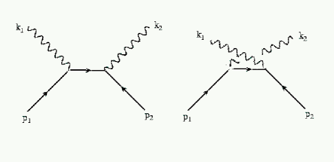
Pair annihilation occurs to lowest order in $\alpha_{em}$ through the two tree-level diagrams shown in Figure 1.

Figure 1: The two lowest order diagrams for pair annihilation.

As in the SM, the spin-averaged squared amplitude is written

$${1\over 4}\sum_{spins}|{\cal M}|^{2} = {e^{4}\over 4}g_{\mu\rho}g_{\nu\sigma}\cdot tr\bigg{\{}(p/_{1}+m)\bigg{[}\frac{\gamma^{\mu}k/_{1}\gamma^{\nu}-2\gamma^{\mu}p_{1}^{\nu}}{2p_{1}\cdot k_{1}}+\frac{\gamma^{\nu}k/_{2}\gamma^{\mu}-2\gamma^{\nu}p_{1}^{\mu}}{2p_{1}\cdot k_{2}}\bigg{]}$$

$$\cdot(p/_{1}+m)\bigg{[}\frac{\gamma^{\sigma}k/_{1}\gamma^{\rho}-2\gamma^{\rho}p_{1}^{\sigma}}{2p_{1}\cdot k_{1}}+\frac{\gamma^{\rho}k/_{2}\gamma^{\sigma}-2\gamma^{\sigma}p_{1}^{\rho}}{2p_{1}\cdot k_{2}}\bigg{]}\bigg{\}}$$

with $m$ the electron mass. Recall the metric tensors are however not as in the SM, but rather $g_{\mu\nu}=\eta_{\mu\nu}+a_{\mu\nu}$ with $a_{\mu\nu}$ defined as in Eqn 4. We defer the full calculation to the Appendix and simply state our result for the differential cross section:

$$\frac{d\sigma}{d\Omega}_{pSM}+\frac{d\sigma}{d\Omega}_{p1}+\frac{d\sigma}{d\Omega}_{p2}$$ (8)

where

$$\frac{d\sigma}{d\Omega}_{pSM} = \frac{\alpha^{2}}{s}\bigg{[}\frac{1+\cos^{2}\theta}{\sin^{2}\theta}\bigg{]}$$

$$\frac{d\sigma}{d\Omega}_{p1} = \epsilon\frac{\alpha^{2}}{s}\bigg{[}\frac{2\cos\theta}{\sin^{2}\theta}+\frac{(\sin\varphi+\cos\varphi)}{\sin\theta}\bigg{]}$$

$$\frac{d\sigma}{d\Omega}_{p2} = 2\epsilon^{2}\frac{\alpha^{2}}{s}\bigg{[}\frac{\cos^{2}\theta-3}{\sin^{2}\theta}+\frac{(1+\cos\theta)\sin 2\theta}{\sin^{4}\theta}(\sin\varphi-\cos\varphi)-\frac{\sin 2\theta}{\sin^{2}\theta}\cos\varphi\bigg{]}$$

Here we are working in the high-energy limit ($m_{e}\approx 0$) and the usual angles $\theta$ and $\varphi$ parameterize photon direction in the center of mass frame. We have written the ${\cal O}(\epsilon)$ and ${\cal O}(\epsilon^{2})$ contributions separately because we will later see in Section 3 that constraints on Lorentz violation strongly favor the scenario where $\epsilon$ (but not necessarily $\epsilon^{2}$) average to zero over small distances. In this case the prediction of NGT for the differential cross section is $\frac{d\sigma}{d\Omega}_{pSM}+\frac{d\sigma}{d\Omega}_{p2}$.

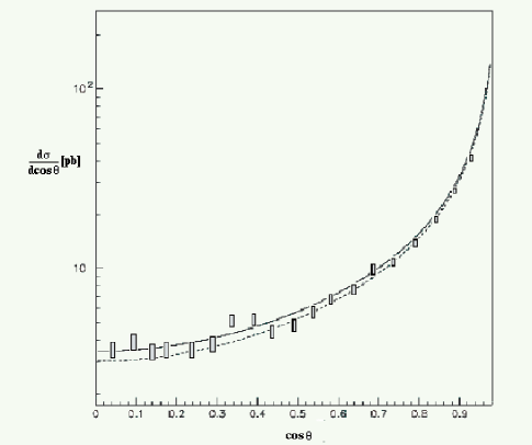
Recently the OPAL Collaboration [10] has analyzed pair annihilation data at a center of mass energy near $200~{}GeV$. In Figure 2 we show their data for the differential cross section $d\sigma/d\cos\theta$ and our prediction $\frac{d\sigma}{d\Omega}_{pSM}+\frac{d\sigma}{d\Omega}_{p2}$. In this case, $\epsilon$ may be as large as $\approx 0.14$ without deviating more than $\sim~{}1~{}\sigma$ with the data.

Figure 2: The OPAL data for $e^{+}e^{-}\to\gamma\gamma$  [10] shown against the predictions in the SM (solid line) and the NGT (dashed line) in the case where odd powers of $\epsilon$ average to zero. Here $\epsilon\approx 0.14$

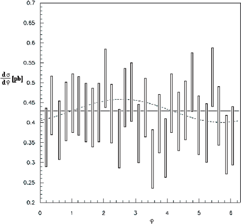
Using this value of $\epsilon$ we predict the azimuthal distribution in Figure 3, again showing the OPAL data alongside the prediction from the SM (in this case a flat line). As one can see from the figure, the data are consistent with both the SM and NGT for this value of $\epsilon$.

The prediction from noncommutative models similarly consists of a negative correction to $d\sigma/d\cos\theta$ and an oscillatory $d\sigma/d\varphi$  [11]. In this case the OPAL data are consistent with $\theta_{\mu\nu}<(141~{}GeV)^{-2}$, to which we refer the reader to the original OPAL report for the details.

Figure 3: Differential cross section in the azimuthal angle from the OPAL data shown against the predictions in the SM (solid line) and the NGT (dashed line) for $\epsilon\approx 0.14$. An angular cut of $cos\theta<0.6$ was applied.

2.2 Bhabha Scattering: $e^{+}e^{-}\to e^{+}e^{-}$

As seen in the previous section, the $d\sigma/d\cos\theta$ distribution for pair annihiliation served to constrain $\epsilon$ more severely than the azimuthal distribution $d\sigma/d\varphi$. Our aim in this and the following section is to see whether other simple scattering processes can add to this constraint.

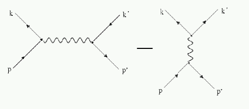
The Bhabha scattering amplitude receives contributions from diagrams involving both the photon and the Z boson as shown in Fig 4.

Figure 4: Tree-level diagrams for Bhabha scattering where the gauge boson is either a photon or a $Z$.

However, it will be simplest to consider this process in the energy range $m_{e}\ll\sqrt{s}\ll m_{Z}$ where we may ignore the $Z$ diagrams and the electron mass. In this limit the differential cross section is approximately (see Appendix for details)

$$\frac{d\sigma}{d\Omega}_{bSM}+\frac{d\sigma}{d\Omega}_{b1}+\frac{d\sigma}{d\Omega}_{b2}$$ (10)

where

$$\frac{d\sigma}{d\Omega}_{bSM} = \frac{\alpha^{2}}{2s}\bigg{[}\frac{1+\cos^{4}\theta/2}{\sin^{4}\theta/2}+\frac{1}{2}(1+\cos^{2}\theta)-2\frac{\cos^{4}\theta/2}{\sin^{2}\theta/2}\bigg{]}$$ (11)

$$\frac{d\sigma}{d\Omega}_{b1} = \epsilon\frac{\alpha^{2}}{s}\left[\frac{\cos^{2}\theta+6\cos\theta-1}{\sin^{2}\theta/2}+\sin\theta(\sin\varphi+\cos\varphi)\right]$$ (13)

$$\frac{d\sigma}{d\Omega}_{b2} = \epsilon^{2}\frac{\alpha^{2}}{2s}\bigg{[}\sin 2\theta(\sin\varphi+\cos\varphi)-\sin^{2}\theta$$ (19)

$$-2\frac{\cos^{2}\frac{\theta}{2}}{\sin^{4}\frac{\theta}{2}}(\sin\theta(\sin\varphi+\cos\varphi)+\cos\theta+1)$$

$$-4\frac{\cos^{2}\frac{\theta}{2}}{\sin^{2}\frac{\theta}{2}}(\sin\theta\cos\varphi-\cos\theta+1)\bigg{]}$$

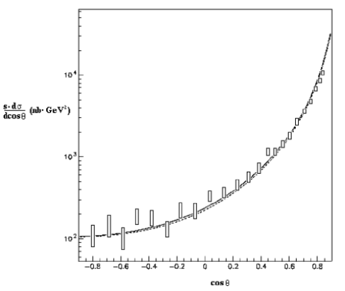
Again we see the characteristic oscillatory dependence on the azimuthal angle, similar to the prediction from noncommutative theories [11]. We can compare the prediction in Eqn 10 (setting $\frac{d\sigma}{d\Omega}_{b1}=0$) with a measurement by the PLUTO Collaboration [12] performed at $\sqrt{s}=9.4~{}GeV$ (see Figure 5). We conclude that for the case of $\epsilon=0.14$ there is no conflict with the data.

Figure 5: Bhabha scattering at $\sqrt{s}=9.4~{}GeV$ as measured by the PLUTO Collaboration [12] plotted alongside the SM prediction(solid line) and the NGT prediction (dashed line) for $\epsilon\approx 0.14$.

2.3 M$\o$ller Scattering: $e^{-}e^{-}\to e^{-}e^{-}$

Finally we consider the constraints from M$\o$ller scattering. Now the differential cross section is (see Appendix)

$$\frac{d\sigma}{d\Omega}_{mSM}+\frac{d\sigma}{d\Omega}_{m1}+\frac{d\sigma}{d\Omega}_{m2}$$ (21)

where

$$\frac{d\sigma}{d\Omega}_{mSM} = \frac{\alpha^{2}}{s}\bigg{[}1+\frac{1}{\sin^{4}\theta/2}+\frac{1}{\cos^{4}\theta/2}\bigg{]}$$ (22)

$$\frac{d\sigma}{d\Omega}_{m1} = -2\epsilon\frac{\alpha^{2}}{s}\bigg{[}\frac{\cos^{2}\theta+6\cos\theta-1}{\sin^{2}\theta/2}+4\frac{\sin^{2}\theta/2}{\sin\theta}(\sin\varphi+\cos\varphi)\bigg{]}$$ (24)

$$\frac{d\sigma}{d\Omega}_{m2} = -8\epsilon^{2}\frac{\alpha^{2}}{s\sin^{4}\theta}\bigg{[}\sin^{4}\theta+\sin\theta\cos\theta((3+\cos^{2}\theta)\sin\varphi+(5-\cos^{2}\theta)\cos\varphi\bigg{]}$$ (26)

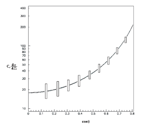
We note a dependence on $\varphi$ similar to that in the other scattering processes and check the constraint from the $\theta$ distribution: Figure 6 shows data taken at the Mark III linear accelerator at SLAC [13]. Again we see that the agreement between theory and experiment is excellent for $\epsilon\approx 0.14$.

Figure 6: M$\o$ller scattering at $\sqrt{s}=600~{}MeV$ at Mark III [13] plotted on the SM prediction(solid line) and the NGT prediction (dashed line) for $\epsilon\approx 0.14$. The cross section is plotted in inverse units of $C_{o}\equiv\frac{1}{8}r_{D}^{2}(\frac{m_{e}}{E})^{2}$.

3 Constraints from General Relativity

We have seen in the previous sections that NGT passes several tests in experiments probing high energies. It is relevant to inquire whether the theory likewise satisfies constraints at energies corresponding to macroscopic or cosmological scales. Thus we leave high energy physics to the side for the moment and concentrate on constraints in the framework of general relativity. Although a fair number of papers address this question we will restrict ourselves to a discussion of only a few of these.

3.1 Newton’s $2^{nd}$ Law

Starting from the geodesic equation in GR,

$$\frac{d^{2}x^{\mu}}{d\sigma^{2}}+\Gamma^{\mu}_{\nu\lambda}\frac{dx^{\nu}}{d\sigma}\frac{dx^{\lambda}}{d\sigma}=0$$ (28)

and using the metric chosen in Eqn (4), we obtain for a particle in a conservative potential $U(x,y,z)$ the following equations of motion:

$$m\frac{d^{2}}{dt^{2}}\left(\begin{array}[]{c}x\\ y\\ z\\ \end{array}\right)=\frac{1}{1-\epsilon^{4}}\left(\begin{array}[]{ccc}-1+\epsilon^{2}&-\epsilon(1-\epsilon^{2})&-\epsilon(1+\epsilon)^{2}\\ \epsilon(1-\epsilon^{2})&-1+\epsilon^{2}&-\epsilon(1-\epsilon^{2})\\ \epsilon(1-\epsilon)^{2}&\epsilon(1-\epsilon^{2})&-1+\epsilon^{2}\\ \end{array}\right)\left(\begin{array}[]{c}U_{x}\\ U_{y}\\ U_{z}\\ \end{array}\right)$$ (29)

where $U_{i}\equiv dU/dx^{i}$. Thus motion in a given direction is influenced by the gradient of the potential in an orthogonal direction, violating Newton’s Second Law. That planets in the solar system move on Keplerian orbits to an excellent approximation puts very stringent constraints on such deviations from $F=ma$. Therefore, if $\epsilon$ varies only slowly over solar-system distances, its magnitude must be vanishingly small to match the observed trajectories of the planets. On the other hand, if $\epsilon$ averages to zero over much smaller distances($\it e.g.$ sub-micron) then odd powers of $\epsilon$ may be set to zero in Eqn (29). The even powers of $\epsilon$ may be removed from off-diagonal entries by a suitable coordinate rotation (see Appendix), reducing Eqn (29) to the usual diagonal form. This is the justification for setting odd powers of $\epsilon$ to zero in the scattering cross section formulae in Eqns 8, 10, and 21.

3.2 Cosmology

Strictly homogeneous and isotropic solutions of the NGT field equations always reduce to the Friedmann-Robertson-Walker(FRW) solutions of GR [3]. Relaxing the homogeneous requirement slightly ($\it i.e.$ turning on $g_{[\mu\nu]}$) leads to the approximate FRW metric

$$ds^{2}=dt^{2}-R^{2}(t)\left(h(r)dr^{2}+r^{2}(d\theta^{2}+\sin^{2}\theta~{}d\varphi^{2})\right)$$ (30)

where the field equations determine $h(r)$ as well as $b(r)$ in the following equation involving the Hubble variable $H=\dot{R}/R$:

$$H^{2}(t)+\frac{b(r)}{R^{2}(t)} = \Omega(r,t)H^{2}(t)$$ (31)

$$\Omega(r,t) \equiv \Omega_{M}(t)+\Omega_{S}(r,t)$$ (32)

$$\Omega_{M}(t) = \frac{8\pi G\rho_{M}(t)}{3H^{2}(t)}$$ (33)

Here $\Omega_{M}(t)$ is the usual matter density while $\Omega_{S}(r,t)$ is the contribution to density from $g_{[\mu\nu]}$. Precise measurements of the curvature and density of the universe can therefore put constraints on the magnitude of $g_{[\mu\nu]}$.

Another way to constrain NGT is by measuring the polarization of light arriving from distant cosmic sources [3]. This can be seen immediately from the electromagnetic action:

$$I_{e}m\sim\int d^{4}x\sqrt{-g}g_{\mu\alpha}g_{\nu\beta}F^{\mu\nu}F^{\alpha\beta}$$ (35)

upon expanding $g$ as in Eqn(1). One can show that terms like $\partial^{i}A^{i}\partial^{j}A^{j},i\neq j$ arise with no counterpart in ordinary electromagnetism. Such terms imply a “mixing” between directions as light propagates, leading to a distance-dependent polarization.

3.3 Astrophysics

Stellar collapse is predicted to differ markedly from the standard GR prediction: namely, a collapsing star with mass above the Chandrasekhar limit does not lead to a black hole singularity [4]. The collapse is found to asymptotically reach a compact pseduo-stable state which, like a black hole, emits larges amounts of thermal and gravitational radiation, but no Hawking radiation. For practical purposes therefore it may be difficult to distinguish this object from a standard GR black hole.

At galactic scales, NGT may provide an explanation for the flat behaviour of rotation curves in spiral galaxies alternative to the conventional theory that the galactic halo consists of $90$ percent dark matter. NGT can alter Newtonian gravity at galactic scales [5], predicting rotation curves in agreement with data, without measurably affecting gravity at or below solar system scales.

We stress that these and other cosmological or astrophysical tests of NGT are just as important as ones performed at high energy such as those considered in this paper. While the latter tests bear results similar to those from noncommutative theories, it is the former which can most clearly distinguish between the two since NGT is a gravitational phenomenon whereas noncommutivity in the conventional string theory context is not.

4 Conclusions

We have seen in the preceding analysis that, in electron scattering experiments, the predictions of NGT are similar to those from theories of noncommuting coordinates. Although in both theories the deviation of the differential cross section $d\sigma/d\theta$ from the SM prediction offers the strongest constraint, we suggest that as experimental precision improves the oscillatory behaviour of $d\sigma/d\varphi$ should be the clearest prediction of these theories since the SM background is flat. We conclude that the OPAL data is consistent with both a ncSM with $\theta_{\mu\nu}\sim(141~{}GeV)^{-2}$ and the particular NGT presented in this paper for values of $\epsilon\sim~{}0.14$, implying that the metric of space-time could be up to $2$ percent antisymmetric in the neighborhood of terrestrial experiments. Precision data from PLUTO and MarkIII confirm the latter bound on NGT. However, in contrast to the parameter $\epsilon$, which is dimensionless, the parameter $\theta_{\mu\nu}$ is of mass dimension $-2$ and therefore should cause deviations from the SM which scale with the square of center-of-mass energy. As more data becomes available from high energy collider experiments such as those planned at the LHC or a future $e^{+}e^{-}$ linear collider, noncommutative signals should therefore grow stronger and eventually overtake those of NGT.

From a theoretical perspective, NGT is a much cleaner theory than the ncSM. The latter, aside from some difficulties in the gauge sector, suffers from severe Lorentz violation and a still unsolved problem in ultraviolet divergences [1]. Nonetheless, both theories represent interesting perturbations of ordinary space-time. Mixing of space-time coordinates is a common feature of both noncommutative theory and NGT, though the origin of this mixing arises from electromagnetism in the former and gravity in the latter. Cosmological and astrophysical phenomenology should therefore readily distinguish the two theories. Work in this area has thus far been encouraging.

Appendix

Useful Identities

The following is a partial list of contractions and trace identities for gamma matrices contracted with $a_{\mu\nu}$.

contraction identities

$$\gamma_{\mu} = (\eta_{\mu\nu}+a_{\mu\nu})\gamma^{\nu}$$ (36)

$$\gamma^{\mu}\gamma_{\mu} = 4+\gamma^{\mu}a_{\mu\nu}\gamma^{\nu}$$ (37)

$$\gamma_{\mu}\gamma^{\mu} = 4-\gamma^{\mu}a_{\mu\nu}\gamma^{\nu}$$ (38)

$$\gamma^{\mu}\gamma^{\nu}\gamma_{\mu} = -2\gamma^{\nu}-\gamma^{\nu}\gamma^{\mu}a_{\mu\rho}\gamma^{\rho}+2\eta^{\nu\mu}a_{\mu\rho}\gamma^{\rho}$$ (39)

$$\gamma_{\mu}\gamma^{\nu}\gamma^{\mu} = -2\gamma^{\nu}+\gamma^{\mu}a_{\mu\rho}\gamma^{\rho}\gamma^{\nu}+2\eta^{\nu\mu}a_{\mu\rho}\gamma^{\rho}$$ (40)

$$\gamma^{\mu}\gamma^{\nu}\gamma^{\rho}\gamma_{\mu} = 4\eta^{\nu\rho}+\gamma^{\nu}\gamma^{\rho}\gamma^{\mu}a_{\mu\lambda}\gamma^{\lambda}+2(\gamma^{\rho}\eta^{\nu\mu}-\gamma^{\nu}\eta^{\rho\mu})a_{\mu\lambda}\gamma^{\lambda}$$ (41)

$$\gamma_{\mu}\gamma^{\nu}\gamma^{\rho}\gamma^{\mu} = 4\eta^{\nu\rho}-\gamma^{\mu}a_{\mu\lambda}\gamma^{\lambda}\gamma^{\nu}\gamma^{\rho}+2(\eta^{\rho\mu}a_{\mu\lambda}\gamma^{\lambda}\gamma^{\nu}-\eta^{\nu\mu}a_{\mu\lambda}\gamma^{\lambda}\gamma^{\rho})$$ (42)

$$\gamma^{\mu}\gamma^{\nu}\gamma^{\rho}\gamma^{\sigma}\gamma_{\mu} = -2\gamma^{\sigma}\gamma^{\rho}\gamma^{\nu}-\gamma^{\nu}\gamma^{\rho}\gamma^{\sigma}\gamma^{\mu}a_{\mu\lambda}\gamma^{\lambda}+2(\gamma^{\nu}\gamma^{\rho}\eta^{\sigma\mu}-\gamma^{\nu}\gamma^{\sigma}\eta^{\rho\mu}+\gamma^{\rho}\gamma^{\sigma}\eta^{\nu\mu})a_{\mu\lambda}\gamma^{\lambda}$$

trace identities

$$tr[\gamma^{\mu}a_{\mu\nu}\gamma^{\nu}] = 0$$ (44)

$$tr[\gamma^{\lambda}a_{\lambda\mu}\gamma^{\nu}] = 4\eta^{\nu\rho}a_{\rho\mu}$$ (45)

$$tr[\gamma^{\mu}a_{\mu\nu}\gamma^{\nu}\gamma^{\sigma}\gamma^{\tau}] = -8\eta^{\sigma\mu}a_{\mu\nu}\eta^{\nu\tau}$$ (46)

$$tr[\gamma^{\mu}a_{\mu\nu}\gamma^{\nu}\gamma^{\rho}\gamma^{\sigma}\gamma^{\tau}\gamma^{\lambda}] = 8(-\eta^{\rho\mu}a_{\mu\nu}\eta^{\nu\sigma}\eta^{\tau\lambda}+\eta^{\rho\mu}a_{\mu\nu}\eta^{\nu\tau}\eta^{\sigma\lambda}-\eta^{\rho\mu}a_{\mu\nu}\eta^{\nu\lambda}\eta^{\sigma\tau}$$

$$-\eta^{\sigma\mu}a_{\mu\nu}\eta^{\nu\tau}\eta^{\rho\lambda}+\eta^{\sigma\mu}a_{\mu\nu}\eta^{\nu\lambda}\eta^{\rho\tau}-\eta^{\tau\mu}a_{\mu\nu}\eta^{\nu\lambda}\eta^{\rho\sigma}$$

Pair Annihilation

To compute the pair annihilation cross section, we may start from the expression for Compton scattering which is related by crossing symmetry ($p_{1}\to p,p_{2}\to-p^{\prime},k_{1}\to-k,k_{2}\to k^{\prime}$):

$$i{\cal M} = \bar{u}(p^{\prime})(-ie\gamma^{\mu})\epsilon^{\ast}_{\mu}(k^{\prime})\frac{i(p/+k/+m)}{(p+k)^{2}-m^{2}}(-ie\gamma^{\nu})\epsilon_{\nu}(k)u(p)$$ (48)

$$+\bar{u}(p^{\prime})(-ie\gamma^{\nu})\epsilon_{\nu}(k)\frac{i(p/-k/^{\prime}+m)}{(p-k^{\prime})^{2}-m^{2}}(-ie\gamma^{\mu})\epsilon^{\ast}_{\mu}(k^{\prime})u(p)$$

$$= -ie^{2}\epsilon^{\ast}_{\mu}(k^{\prime})\epsilon_{\nu}(k)\bar{u}(p^{\prime})\bigg{[}\frac{\gamma^{\mu}(p/+k/+m)\gamma^{\nu}}{(p+k)^{2}-m^{2}}+\frac{\gamma^{\nu}(p/-k/^{\prime}+m)\gamma^{\mu}}{(p-k^{\prime})^{2}-m^{2}}\bigg{]}u(p)$$

From here, the cross section is

$${1\over 4}\sum_{spins}|{\cal M}|^{2} = {e^{4}\over 4}g_{\mu\rho}g_{\nu\sigma}\cdot tr\bigg{\{}(p/^{\prime}+m)\bigg{[}\frac{\gamma^{\mu}k/\gamma^{\nu}+2\gamma^{\mu}p^{\nu}}{2p\cdot k}+\frac{\gamma^{\nu}k/^{\prime}\gamma^{\mu}-2\gamma^{\nu}p^{\mu}}{2p\cdot k^{\prime}}\bigg{]}$$ (49)

$$\cdot(p/+m)\bigg{[}\frac{\gamma^{\sigma}k/\gamma^{\rho}+2\gamma^{\rho}p^{\sigma}}{2p\cdot k}+\frac{\gamma^{\rho}k/^{\prime}\gamma^{\sigma}-2\gamma^{\sigma}p^{\rho}}{2p\cdot k^{\prime}}\bigg{]}\bigg{\}}$$

$$\equiv {e^{4}\over 4}\bigg{[}\frac{I}{(2p\cdot k)^{2}}+\frac{II}{(2p\cdot k)(2p\cdot k^{\prime})}+\frac{III}{(2p\cdot k^{\prime})(2p\cdot k)}+\frac{IV}{(2p\cdot k^{\prime})^{2}}\bigg{]}$$

where the first trace is

$$I = tr[(p/^{\prime}+m)(\gamma^{\mu}k/\gamma^{\nu}+2\gamma^{\mu}p^{\nu})(p/+m)(\gamma_{\nu}k/\gamma_{\mu}+2\gamma_{\mu}p_{\nu})]$$

First we consider the ${\cal O}(\epsilon)$ contributions to this amplitude. In the computation we will need to insert the full expression for $g_{\mu\nu}$ only; note that to leading order Dirac propagators are unchanged, $\it e.g.$ $\Sigma_{s}u(p)\overline{u}_{s}(p)=p/+m\equiv p^{\mu}\eta_{\mu\nu}\gamma^{\nu}+m$, which is true even after radiative corrections. After much Dirac algebra using the contraction and trace identities above and taking the high energy limit $m=0$, we find that $I$ has no ${\cal O}(\epsilon)$ piece. However the second trace,

$$II = tr[(p/^{\prime}+m)(\gamma^{\mu}k/\gamma^{\nu}+2\gamma^{\mu}p^{\nu})(p/+m)(\gamma_{\mu}k/^{\prime}\gamma_{\nu}-2\gamma_{\nu}p_{\mu})]$$

$$= tr[p/^{\prime}\gamma^{\mu}k/\gamma^{\nu}p/\gamma_{\mu}k/^{\prime}\gamma_{\nu}]-2tr[p/^{\prime}\gamma^{\mu}k/\gamma^{\nu}p/\gamma_{\nu}p_{\mu}]$$

$$+mtr[p/^{\prime}\gamma^{\mu}k/\gamma^{\nu}\gamma_{\mu}k/^{\prime}\gamma_{\nu}]-2mtr[p/^{\prime}\gamma^{\mu}k/\gamma^{\nu}\gamma_{\nu}p_{\mu}]$$

$$+2tr[p/^{\prime}\gamma^{\mu}p^{\nu}p/\gamma_{\mu}k/^{\prime}\gamma_{\nu}]-4tr[p/^{\prime}\gamma^{\mu}p^{\nu}p/\gamma_{\nu}p_{\mu}]$$

$$+2mtr[p/^{\prime}\gamma^{\mu}p^{\nu}\gamma_{\mu}k/^{\prime}\gamma_{\nu}]-4mtr[p/^{\prime}\gamma^{\mu}p^{\nu}\gamma_{\nu}p_{\mu}]$$

$$+mtr[\gamma^{\mu}k^{\prime}/\gamma^{\nu}\gamma_{\mu}k/^{\prime}\gamma_{\nu}]-2mtr[\gamma^{\mu}k/\gamma^{\nu}p/\gamma_{\nu}p_{\mu}]$$

$$+m^{2}tr[\gamma^{\mu}k/\gamma^{\nu}\gamma_{\mu}k/^{\prime}\gamma_{\nu}]-2m^{2}tr[\gamma^{\mu}k/\gamma^{\nu}\gamma_{\nu}p_{\mu}]$$

$$+2mtr[\gamma^{\mu}p^{\nu}p/\gamma_{\mu}k/^{\prime}\gamma_{\nu}]-4mtr[\gamma^{\mu}p^{\nu}p/\gamma_{\nu}p_{\mu}]$$

$$+2m^{2}tr[\gamma^{\mu}p^{\nu}\gamma_{\mu}k/^{\prime}\gamma_{\nu}]-4m^{2}tr[\gamma^{\mu}p^{\nu}\gamma_{\nu}p_{\mu}]$$

$$= tr[p/^{\prime}\gamma^{\mu}k/\gamma^{\nu}p/\gamma_{\mu}k/^{\prime}\gamma_{\nu}]-2tr[p/^{\prime}\gamma^{\mu}k/\gamma^{\nu}p/\gamma_{\nu}p_{\mu}]$$

$$+2tr[p/^{\prime}\gamma^{\mu}p^{\nu}p/\gamma_{\mu}k/^{\prime}\gamma_{\nu}]-4tr[p/^{\prime}\gamma^{\mu}p^{\nu}p/\gamma_{\nu}p_{\mu}]$$

yields

$$II =$$ ordinary theory (52)

$$-32\epsilon p^{\prime}\cdot pk\oslash k^{\prime}+16\epsilon(p\cdot kp\oslash p^{\prime}+p^{\prime}\cdot pk\oslash p)$$

where we define

$$p\cdot k \equiv p_{\mu}\eta^{\mu\nu}k_{\nu}$$

$$p\oslash k \equiv p_{\mu}\eta^{\mu\nu}a_{\nu\rho}\eta^{\rho\sigma}k_{\sigma}$$

and “ordinary theory” refers to the SM ($\epsilon=0$). The other traces are trivially obtained from the above:

$$III=II$$

$$IV=I(k\rightarrow-k^{\prime})$$ (54)

Transforming to the pair annihiliation momenta by crossing symmetry,

$$p\rightarrow p_{1},p^{\prime}\rightarrow-p_{2},k\rightarrow-k_{1},k^{\prime}\rightarrow k_{2}$$ (55)

we obtain

$${1\over 4}\sum_{spins}|{\cal M}|^{2} \equiv {e^{4}\over 4}\bigg{[}\frac{I}{(2p_{1}\cdot k_{1})^{2}}-\frac{II}{(2p_{1}\cdot k_{1})(2p_{1}\cdot k_{2})}-\frac{III}{(2p_{1}\cdot k_{2})(2p_{1}\cdot k_{1})}+\frac{IV}{(2p_{1}\cdot k_{2})^{2}}\bigg{]}$$

and

$$II = III$$ (57)

$$=$$ ordinary theory

$$-32\epsilon p_{2}\cdot p_{1}k_{1}\oslash k_{2}+16\epsilon(p_{1}\cdot k_{1}p_{1}\oslash p_{2}+p_{2}\cdot p_{1}k_{1}\oslash p_{1})$$

$$I =$$ ordinary theory (58)

$$IV =$$ ordinary theory (59)

Define the kinematical variables $E,\theta,\varphi$ in the center of mass frame:

$$p_{1}=(E,E\hat{z})$$

$$p_{2}=(E,-E\hat{z})$$

$$k_{1}=(E,E\sin\theta\cos\varphi,E\sin\theta\sin\varphi,E\cos\theta)$$

$$k_{2}=(E,-E\sin\theta\cos\varphi,-E\sin\theta\sin\varphi,-E\cos\theta)$$ (60)

It is now straightforward to derive the ${\cal O}(\epsilon)$ differential cross section:

$$\frac{d\sigma}{d\Omega} =$$ ordinary theory

$$+\frac{\alpha^{2}\epsilon}{2E^{2}}\cdot\bigg{[}\frac{2\cos\theta}{\sin^{2}\theta}+\frac{(\sin\varphi+\cos\varphi)}{\sin\theta}\bigg{]}$$

Now for ${\cal O}(\epsilon^{2})$: The first trace eventually reduces to

$$I = 32[p\cdot kp^{\prime}\otimes k+p^{\prime}\cdot kp\otimes k-p^{\prime}\cdot pk\otimes k]$$ (62)

$$-32p^{\prime}\oslash kp\oslash k-16tr(a^{2})p^{\prime}\cdot kp\cdot k$$

where we introduce the notation $\otimes$:

$$k\otimes p = k_{\mu}\eta^{\mu\nu}a_{\nu\rho}\eta^{\rho\sigma}a_{\sigma\tau}\eta^{\tau\lambda}p_{\lambda}=p\otimes k$$

$$tr(a^{2}) = \eta^{\mu\nu}a_{\nu\rho}\eta^{\rho\sigma}a_{\sigma\tau}\eta^{\tau}_{\cdot\mu}$$

Similarly, the second trace is

$$II = 16\epsilon^{2}(k^{\prime}\otimes kp^{\prime}\cdot p+p^{\prime}\otimes pk^{\prime}\cdot k)$$

Then the other traces follow easily as before:

$$III = II=16\epsilon^{2}(k^{\prime}\otimes kp^{\prime}\cdot p+p^{\prime}\otimes pk^{\prime}\cdot k)$$ (65)

$$IV = I(k\rightarrow-k^{\prime})=32[p\cdot k^{\prime}p^{\prime}\otimes k^{\prime}+p^{\prime}\cdot k^{\prime}p\otimes k^{\prime}-p^{\prime}\cdot pk^{\prime}\otimes k^{\prime}]$$ (66)

$$-32p^{\prime}\oslash k^{\prime}p\oslash k^{\prime}-16tr(a^{2})p^{\prime}\cdot k^{\prime}p\cdot k^{\prime}$$

From the particular choice of $a$ in Eqn 4, we have

$$a_{\nu\rho}\eta^{\rho\sigma}a_{\sigma\tau} = \left(\begin{array}[]{cccc}3&2&0&-2\\ 2&1&0&-2\\ 0&0&1&0\\ -2&-2&0&1\end{array}\right)$$ (71)

whence it follows from the kinematical assignments that

$${1\over 4}\sum_{spins}|{\cal M}|^{2} = {\rm ordinary}+{\cal O}(\epsilon)+4e^{4}\epsilon^{2}\bigg{[}\frac{\cos^{2}\theta-3}{\sin^{2}\theta}+\frac{(1+\cos\theta)\sin 2\theta}{\sin^{4}\theta}(\sin\varphi-\cos\varphi)-\frac{\sin 2\theta}{\sin^{2}\theta}\cos\varphi\bigg{]}$$

leading to the expression reported in Eqn 8.

Bhabha Scattering

The two diagrams contributing (see Figure 4) interfere destructively, with spin averaged squared amplitude

$${1\over 4}\sum_{spins}|{\cal M}|^{2} = \frac{e^{4}}{4}\bigg{[}\frac{I}{(p+p^{\prime})^{4}}+\frac{II}{(k^{\prime}-p^{\prime})^{4}}-\frac{III+IV}{(p+p^{\prime})^{2}(k^{\prime}-p^{\prime})^{2}}\bigg{]}$$

$$I \equiv tr[p/^{\prime}\gamma^{\mu}p/\gamma^{\sigma}]tr[k/\gamma^{\nu}k/^{\prime}\gamma^{\rho}]g_{\mu\nu}g_{\rho\sigma}$$

$$II \equiv I(p\leftrightarrow k^{\prime})$$

$$III \equiv tr[p/^{\prime}\gamma^{\mu}p/\gamma^{\rho}k/\gamma^{\nu}k/^{\prime}\gamma^{\sigma}]g_{\mu\nu}g_{\rho\sigma}$$

$$IV \equiv III(p\leftrightarrow k^{\prime})$$

Then

$$I = p^{\prime}_{\alpha}p_{\beta}(\eta^{\alpha\mu}\eta^{\beta\sigma}-\eta^{\alpha\beta}\eta^{\mu\sigma}+\eta^{\alpha\sigma}\eta^{\mu\beta})\oslash k_{\lambda}k^{\prime}_{\tau}(\eta^{\lambda\nu}\eta^{\tau\rho}-\eta^{\lambda\tau}\eta^{\nu\rho}+\eta^{\lambda\rho}\eta^{\nu\tau})g_{\mu\nu}g_{\rho\sigma}$$

$$= {\rm ordinarytheory}+$$

$$-2\bigg{[}(p\oslash k^{\prime})(p^{\prime}\oslash k)+(p^{\prime}\oslash k^{\prime})(p\oslash k)+(k\cdot k^{\prime})(p\otimes p^{\prime})\bigg{]}$$

($\it i.e.$ there is no ${\cal O}(\epsilon)$ piece). By repeated use of the contraction identities noted earlier, one can further verify that

$$III+IV = {\rm ordinary~{}theory}+32\bigg{[}(p\cdot p^{\prime})(k\oslash k^{\prime})+(p^{\prime}\cdot k^{\prime})(k\oslash p)+(p\cdot k^{\prime})(p^{\prime}\otimes k)-(k\cdot p^{\prime})(k^{\prime}\otimes p)\bigg{]}$$

Using the kinematical assignments as in Eqn Pair Annihilation, replacing $p_{1}\to p,p_{2}\to p^{\prime},k_{1}\to k,k_{2}\to k^{\prime}$, the quoted cross section in the text follows straightforwardly.

M$\o$ller Scattering

This can be obtained quickly from Bhabha scattering by substituting $p$ for $k$ and vice versa in the traces ( but not in the denominators). Hence

$${1\over 4}\sum_{spins}|{\cal M}|^{2} = \frac{e^{4}}{4}\bigg{[}\frac{I}{(p+p^{\prime})^{4}}+\frac{II}{(k^{\prime}-p^{\prime})^{4}}-\frac{III+IV}{(p+p^{\prime})^{2}(k^{\prime}-p^{\prime})^{2}}\bigg{]}$$

where

$$I = {\rm ordinary~{}theory}+$$

$$-2\bigg{[}(k\oslash k^{\prime})(p^{\prime}\oslash p)+(p^{\prime}\oslash k^{\prime})(k\oslash p)+(p\cdot k^{\prime})(k\otimes p^{\prime})\bigg{]}$$

$$II = I(k\leftrightarrow k^{\prime})$$

$$III+IV = {\rm ordinary~{}theory}+32\bigg{[}(k\cdot p^{\prime})(p\oslash k^{\prime})+(p^{\prime}\cdot k^{\prime})(k\oslash p)+(k\cdot k^{\prime})(p^{\prime}\otimes p)-(p\cdot p^{\prime})(k^{\prime}\otimes k)\bigg{]}$$

Making the same kinematical assignments as for Bhabha scattering, the quoted cross section in Section 2.3 follows.

Preserving $F=ma$

Starting from Eqn(29), perform a rotation in the $x-z$ plane:

$$\frac{d^{2}}{dt^{2}}\left(\begin{array}[]{c}x^{\prime}\\ y^{\prime}\\ z^{\prime}\\ \end{array}\right)={\bf\Omega}\left(\begin{array}[]{c}U_{x}^{\prime}\\ U_{y}^{\prime}\\ U_{z}^{\prime}\\ \end{array}\right)$$ (78)

where

$${\bf\Omega}=\frac{1}{1-\epsilon^{4}}\left(\begin{array}[]{ccc}\epsilon^{2}-1-4\epsilon^{2}c_{\theta}s_{\theta}&\frac{1-\epsilon^{4}}{1+\epsilon^{2}}\epsilon(s_{\theta}-c_{\theta})&\epsilon(1+2\epsilon(c^{2}_{\theta}-s^{2}_{\theta})+\epsilon^{2})\\ -\frac{1-\epsilon^{4}}{1+\epsilon^{2}}\epsilon(s_{\theta}-c_{\theta})&-\frac{1-\epsilon^{4}}{1+\epsilon^{2}}&-\frac{1-\epsilon^{4}}{1+\epsilon^{2}}\epsilon(s_{\theta}+c_{\theta})\\ -\epsilon(1+2\epsilon(s^{2}_{\theta}-c^{2}_{\theta})+\epsilon^{2})&\epsilon\frac{1-\epsilon^{4}}{1+\epsilon^{2}}&\epsilon^{2}-1+4\epsilon^{2}c_{\theta}s_{\theta}\\ \end{array}\right)$$ (79)

Neglecting odd powers of $\epsilon$, this can clearly be brought to diagonal form by setting $c_{\theta}=s_{\theta}$, $\it i.e.$ rotating by 45 degrees.