hep-ph/0305237

Saclay t03/061

Gauge Theories on an Interval: Unitarity without a Higgs

Csaba Csáki^a, Christophe Grojean^b, Hitoshi Murayama^c,
Luigi Pilo^b and John Terning^d

^a Newman Laboratory of Elementary Particle Physics
Cornell University, Ithaca, NY 14853, USA

^b Service de Physique Théorique, CEA Saclay, F91191 Gif–sur–Yvette, France

^c Department of Physics, University of California at Berkeley and
Lawrence Berkeley National Laboratory, Berkeley, CA 94720, USA

^d Theory Division T-8, Los Alamos National Laboratory, Los Alamos, NM 87545, USA

csaki@mail.lns.cornell.edu, grojean@spht.saclay.cea.fr, murayama@lbl.gov, pilo@spht.saclay.cea.fr, terning@lanl.gov

We consider extra dimensional gauge theories on an interval. We first review the derivation of the consistent boundary conditions (BC’s) from the action principle. These BC’s include choices that give rise to breaking of the gauge symmetries. The boundary conditions could be chosen to coincide with those commonly applied in orbifold theories, but there are many more possibilities. To investigate the nature of gauge symmetry breaking via BC’s we calculate the elastic scattering amplitudes for longitudinal gauge bosons. We find that using a consistent set of BC’s the terms in these amplitudes that explicitly grow with energy always cancel without having to introduce any additional scalar degree of freedom, but rather by the exchange of Kaluza–Klein (KK) gauge bosons. This suggests that perhaps the SM Higgs could be completely eliminated in favor of some KK towers of gauge fields. We show that from the low-energy effective theory perspective this seems to be indeed possible. We display an extra dimensional toy model, where BC’s introduce a symmetry breaking pattern and mass spectrum that resembles that in the standard model.

1 Introduction

A crucial ingredient of the standard model of particle physics is the Higgs scalar. One of the main arguments for the existence of the Higgs is [1, 2, 3, 4, 5] that without it the scattering amplitude for the longitudinal components of the massive $W$ and $Z$ bosons would grow with energy as $\sim E^{2}$, and thus violate unitarity at energies of order $4\pi M_{W}/g\sim 1.5$ TeV. It has been shown in [6, 7] that higher dimensional gauge theories maintain unitarity in the sense that the terms in the amplitude that would grow with energies as $E^{4}$ or $E^{2}$ cancel (though the theory itself becomes strongly interacting at a cutoff scale which depends on the size of the extra dimension and the effective gauge coupling, and usually tree-level unitarity also breaks down at a scale related to the cutoff scale due to the growing number of KK modes that can contribute to the constant pieces of certain amplitudes). For a related discussion see [8]. This on its own is not so surprising, since one would naively expect that higher dimensional gauge theories behave well in the energy range where they can be valid effective theories. However, such higher dimensional theories can also be used to break the gauge symmetries if one compactifies the theory on an interval instead of a circle. Then by assigning non-trivial boundary conditions (BC’s) to the gauge fields at the endpoints of the interval one can reduce the number of unbroken gauge symmetries, and thus effectively generate gauge boson masses even for the modes that would remain massless when only Neumann BC’s are imposed. This then raises the question, whether the cancellation in the scattering amplitudes of the terms that grow with energy is maintained or not in the presence of such breaking of gauge symmetries. This issue is related to the question of whether the breaking of gauge invariance via boundary conditions is soft or hard. We would like to give a general analysis of this question (which also have been recently addressed in some particular examples in Refs. [9, 10], see also [11] for a related discussion in the case of KK gravity).

In this paper we investigate the nature of gauge symmetry breaking via BC’s. First we review the derivation of the set of equations that the boundary conditions have to obey in order to minimize the action, including a discussion of the issue of gauge fixing. The possible set of BC’s (BC’s) include the commonly considered orbifold BC’s [12, 13, 14, 15] but as it was already noted in [14] there are more possibilities. For example, it is easy to reduce the rank of the gauge group with more general BC’s [14]. The question that such theories raise is whether such a breaking of the gauge symmetries via BC’s yields a consistent theory or not. Since we are insisting that the BC’s be consistent with the variation of a gauge invariant Lagrangian that has no explicit gauge symmetry breaking, one would guess that such breaking should be soft. In order to verify this, we investigate in detail the issue of unitarity of scattering amplitudes in such 5D gauge theories compactified on an interval, with non-trivial BC’s. We derive the general expression for the amplitude for elastic scattering of longitudinal gauge bosons, and write down the necessary conditions for the cancellation of the terms that grow with energy. We find that all the consistent BC’s are unitary in the sense that all terms proportional to $E^{4}$ and $E^{2}$ vanish. In fact, any theory with only Dirichlet or Neumann BC’s is unitary. Surprisingly, this would also include theories where the boundary conditions can be thought of as coming from a very large expectation value of a brane localized Higgs field, in the limit when the expectation value diverges. For such theories with “mixed” BC’s, even when the $E^{4}$ terms cancel, the $E^{2}$ term in the amplitude does not cancel in general. This is not surprising, since such mixed BC’s would generically come from an explicit mass term for the gauge field localized on the boundary. Thus cancellation of the $E^{2}$ term would happen only, if the explicit mass term is completed into a gauge invariant scalar mass term, in which case the exchange of these boundary scalar fields themselves have to be included in order to recover a good high-energy behavior for the theory. Indeed, we find that in some cases it may be possible to introduce such boundary degrees of freedom which would exactly enforce the given BC’s, and their contribution cancels the remaining amplitudes that grow with energy.

These arguments suggest that it should be possible to build an effective theory which has no Higgs field present at all, but where the unitarity of gauge boson scattering amplitudes is ensured by the presence of additional massive gauge fields. We show a simple example of an effective theory of this sort where a single KK mode for the $W$’s and the $Z$ is needed to ensure unitarity, and which are sufficiently heavy and sufficiently weakly coupled to have evaded direct detection and would not have contributed much to electroweak precision observables.

In order to actually make an effective theory of this sort appealing one would have to give a UV completion, for example at least in terms of an extra dimensional theory. Therefore, we will consider several toy models of symmetry breaking with extra dimensions. The first two models are prototype examples of orbifold vs. brane Higgs breaking of symmetries, which we combine in the final semi-realistic model based on the breaking of a left-right symmetric model by an orbifold using an outer automorphism. This model is similar to the standard model, in that it has unbroken electromagnetism, the lightest massive gauge bosons resemble the $W$ and the $Z$, and their mass ratio could be close to a realistic one. However, the masses of the KK modes are too light, and their couplings too strong. Nevertheless, we view this model as a step toward a realistic theory of electroweak symmetry breaking without a Higgs boson.

2 Gauge Theories on an Interval: Consistent BC’s

We consider a theory with a single extra dimension compactified on an interval with endpoints $0$ and $\pi R$. We want to study in this section what are the possible BC’s that the bulk gauge fields have to satisfy. We denote the bulk gauge fields by $A_{M}^{a}(x,y)$, where $a$ is the gauge index, $M$ is the Lorentz index $0,1,2,3,5$, $x$ is the coordinate of the ordinary four dimensions and $y$ is the coordinate along the extra dimension (we will use from time to time a prime to denote a derivative with respect to the $y$ coordinate). We will assume a flat space-time background. We will consider several cases in this section. First we will look at the simplest example of a scalar field in the bulk, which does not have any of the complications of gauge invariance and gauge fixing. Then we will look at pure 5D Yang-Mills theory on an interval. The cases of gauge theory with a bulk or brane scalar field are discussed in Appendix A.

2.1 Bulk scalar

To start out, let us consider a bulk scalar $\phi$ field on an interval with an action

$$\mathcal{S}=\int d^{4}x\,\int_{0}^{\pi R}dy\left(\frac{1}{2}\partial^{{}_{N}}\phi\partial_{{}^{N}}\phi-V(\phi)\right)+\int_{y=0}d^{4}x\,\frac{1}{2}\phi^{2}\,M_{1}^{2}+\int_{y=\pi R}d^{4}x\,\frac{1}{2}\phi^{2}\,M_{2}^{2}\,.$$ (2.1)

In order to find the consistent set of BC’s we impose that the variation of (2.1) vanishes. Varying the action and integrating by parts we get

$$\delta\mathcal{S}= -\int d^{4}x\,\int_{0}^{\pi R}dy\;\delta\phi\,\left(\Box_{5}\phi+\frac{\partial V}{\partial\phi}\right)-$$ (2.2)

$$\int d^{4}x\left(\delta\phi\left(\partial_{5}\phi+M^{2}_{1}\,\phi\right)\big{|}_{\pi R}-\delta\phi\left(\partial_{5}\phi+M^{2}_{2}\,\phi\right)\big{|}_{0}\right)=0\,.$$

Note, that we kept the boundary terms obtained from integrating by parts along the finite extra dimension, while we have assumed as usual that the fields and their derivatives die off as $x_{\mu}\to\infty$. The variation of the bulk terms will give the usual bulk equation of motion

$$\Box_{5}\phi+\frac{\partial V}{\partial\phi}=0.$$ (2.3)

In order to ensure that the action is minimized, one also has to ensure that the variation of the action from the boundary pieces also vanish:

$$\delta\phi\left(\partial_{5}\phi+M^{2}_{i}\,\phi\right)\big{|}_{0,\pi R}=0.$$ (2.4)

A consistent BC is one that automatically enforces the above equation. There are two ways to solve this equation: either the variation of the field on the boundaries is zero, or the expression multiplying the variation. Therefore the consistent set of BC’s that respects 4D Lorentz invariance at $y=0,\pi R$ are

$${\rm({\it i})} \left(\partial_{5}\phi+M^{2}_{i}\,\phi\right)|_{y=0,\pi R}=0\,;$$ (2.5)

$${\rm({\it ii})} \phi|_{y=0,\pi R}=const.\,.$$ (2.6)

Eq. (2.5) corresponds to a mixed BC and it reduces to Neumann for vanishing boundary mass $M^{2}_{i}$; the value of $\phi$ at $y=0,\pi R$ is not specified. The second type of BC corresponds to fixing the values of $\phi$ on the boundary, and reduces to a Dirichlet BC when $const.=0$. It is a matter of choice which one of these conditions one is imposing on the boundaries. One could pick one of these conditions at $y=0$ and the other at $y=\pi R$. When several scalar fields are present, there is also the more interesting possibility to cancel the sum of all the boundary terms without having to require that individually each term is vanishing by itself. We will see an example for this in Section 6 of this paper.

2.2 Pure gauge theory in the bulk

In this case the 5D gauge boson will decompose into a 4D gauge boson $A_{\mu}^{a}$ and a 4D scalar $A_{5}^{a}$ in the adjoint representation. Since there is a quadratic term mixing $A_{\mu}$ and $A_{5}$ we need to add a gauge fixing term that eliminates this cross term. Thus we write the action after gauge fixing in R_ξ gauge as

$$\mathcal{S}=\int d^{4}x\,\int_{0}^{\pi R}dy\left(-\frac{1}{4}F_{\mu\nu}^{a}F^{a\mu\nu}-\frac{1}{2}F_{5\nu}^{a}F^{a5\nu}-\frac{1}{2\xi}(\partial_{\mu}A^{a\mu}-\xi\partial_{5}A_{5}^{a})^{2}\right),$$ (2.7)

where $F^{a}_{MN}=\partial_{M}A_{N}^{a}-\partial_{N}A_{M}^{a}+g_{5}f^{abc}\,A^{b}_{M}A^{c}_{N}$, and the $f^{abc}$’s are the structure constants of the gauge group. The gauge fixing term is chosen such that (as usual) the cross terms between the 4D gauge fields $A_{\mu}^{a}$ and the 4D scalars $A_{5}^{a}$ cancel (see also [17]). Taking $\xi\to\infty$ will result in the unitary gauge, where all the KK modes of the scalars fields $A^{a}_{5}$ are unphysical (they become the longitudinal modes of the 4D gauge bosons), except if there is a zero mode for the $A_{5}$’s. We will assume that every $A_{5}^{a}$ mode is massive, and thus that all the $A_{5}$’s are eliminated in unitary gauge.

The variation of the action (2.7) leads, as usual after integration by parts, to the bulk equations of motion as well as to boundary terms (we denote by $[F]$ the boundary quantity $F(\pi R)-F(0)$):

$$\delta\mathcal{S} = \int d^{4}x\,dy\left(\partial_{M}F^{aM\nu}-g_{5}f^{abc}\,F^{bM\nu}A_{M}^{c}+\frac{1}{\xi}\partial^{\nu}\partial^{\sigma}A_{\sigma}^{a}-\partial^{\nu}\partial_{5}A_{5}^{a}\right)\delta A_{\nu}^{a}$$ (2.8)

$$-\int d^{4}x\,dy\left(\partial^{\sigma}F^{a}_{\sigma 5}-g_{5}f^{abc}\,F^{b}_{\sigma 5}A^{c\sigma}+\partial_{5}\partial_{\sigma}A^{a\sigma}-\xi\partial^{2}_{5}A^{a}_{5}\right)\delta A^{a}_{5}$$

$$+\int d^{4}x\left(\left[F^{a}_{5\nu}\,\delta A^{a\nu}\right]+\left[(\partial_{\sigma}A^{a\sigma}-\xi\partial_{5}A^{a}_{5})\delta A^{a}_{5}\right]\right).$$

The bulk terms will give rise to the usual bulk equations of motion:

$$\partial_{M}F^{aM\nu}-g_{5}f^{abc}\,F^{bM\nu}A_{M}^{c}+\frac{1}{\xi}\partial^{\nu}\partial^{\sigma}A_{\sigma}^{a}-\partial^{\nu}\partial_{5}A_{5}^{a}=0,$$

$$\partial^{\sigma}F^{a}_{\sigma 5}-g_{5}f^{abc}\,F^{b}_{\sigma 5}A^{c\sigma}+\partial_{5}\partial_{\sigma}A^{a\sigma}-\xi\partial^{2}_{5}A^{a}_{5}=0.$$ (2.9)

However, one has to ensure that the variation of the boundary pieces vanish as well. This will lead to the requirements

$$F^{a}_{\nu 5}\,\delta A^{a\nu}{}_{|0,\pi R}=0,$$ (2.10)

$$(\partial_{\sigma}A^{a\sigma}-\xi\partial_{5}A^{a}_{5})\delta A^{a}_{5}{}_{|0,\pi R}=0.$$ (2.11)

The BC’s have to be such that the above equations be satisfied. For example, one can fix all the variations of the fields to vanish at the endpoints, in that case the above boundary terms are clearly vanishing. However, one can also instead of setting $\delta A^{a}_{5}{}_{|0,\pi R}=0$ require that its coefficient $\partial_{\sigma}A^{a\sigma}-\xi\partial_{5}A^{a}_{5}$ vanishes. The different choices lead to different consistent BC’s for the gauge theory on an interval. There are different generic choices of BC that ensure the cancellation of variation at the boundary and preserve 4D Lorentz invariance:

$${\rm({\it i})} A^{a}_{\mu|}=0,A^{a}_{5|}=const.\ ;$$ (2.12)

$${\rm({\it ii})} A^{a}_{\mu|}=0,\partial_{5}A^{a}_{5|}=0\ ;$$ (2.13)

$${\rm({\it iii})} \partial_{5}A^{a}_{\mu|}=0,A^{a}_{5|}=const.\ .$$ (2.14)

However, besides these general choices where the individual terms in the sum of (2.11) vanish, there could be more interesting situations where only the sum of the terms in (2.11) vanish. We will see an example for this in Section 6 of this paper. While conditions (2.12) and (2.13) are exact, condition (2.14) only satisfies Eq. (2.11) to linear order. The exact solution requires $F^{a}_{\nu 5}=0$ which imposes additional constraints especially in the case of an unbroken gauge symmetry (i.e. zero mode gauge fields).

Generically, it is a choice which of these BC’s one wants to impose. One can impose a different type of condition for every different field, meaning for the different colors $a$ and for $A_{\mu}$ vs. $A_{5}$, as long as certain consistency conditions related to the gauge invariance of massless gauge fields is obeyed. Different choices correspond to different physical situations. An analogy for this is the theory of a vibrating rod. The equation of motion is obtained from a variational principle minimizing the total mechanical energy, including the terms appearing from the boundaries. Which of the BC’s one chooses depends on the physical circumstances at its ends: if it is fixed at both ends the BC is clearly that the displacement at the endpoints is zero. However, if it is fixed only on one end, then one will get a non-trivial equation that the displacement on the boundaries has to satisfy, the analog of which is the condition $F^{a}_{\nu 5}=$ in (2.11).

Similarly in the case of gauge theories, it is our choice what kind of physics we are prescribing at the boundaries, as long as the variations of the boundary terms vanish. A priori, one can impose different BC’s for different gauge directions. However, some consistency conditions on the gauge structure may exist. For instance, if one wants to keep a massless vector, then in order to preserve 4D Lorentz invariance the action should possess a gauge invariance. This means that the massless gauge bosons should form a subgroup of the 5D gauge group.

One should note that there is a wider web of consistent BC’s than the one encountered in orbifold theories. For instance, within each gauge direction, the BC (2.12) would have never been consistent with the reflection symmetry $y\to-y$ symmetry of an orbifold. The full gauge structure of the BC’s is also much less constrained: in orbifold theories, the gauge structure was dictated by the use of an automorphism of the Lie algebra, which was a serious obstacle in achieving a rank reducing symmetry breaking. As we will see explicitly in Sections 5.2 and 6, these difficulties are easily alleviated when considering the most general BC’s (2.12)-(2.14).

In order to actually quantize the theory one also needs to add the Faddeev–Popov ghosts to the theory. One can add 5D FP ghost fields $c^{a}$ and $\bar{c}^{a}$ using the gauge fixing function from (2.7)

$${\cal L}_{FP}=\bar{c}^{a}\left(-(\partial_{\mu}D^{\mu})^{ab}+\xi(\partial_{5}D_{5})\right)c^{b}$$ (2.15)

The ghost fields have their own boundary conditions as well.

The cases for gauge theories with bulk scalars or localized scalars are discussed in Appendix A. For the case of a scalar localized at the endpoint the generic form of the BC for the gauge fields (in unitary gauge) will be of the form

$$\partial_{5}A_{\mu}^{a}{}_{|0,\pi R}=V_{0,\pi R}^{ab}A^{b}_{\mu}{}_{|0,\pi R}.$$ (2.16)

These are mixed BC’s that still ensure the hermiticity (self-adjointness) of the Hamiltonian. In the limit $V^{ab}\rightarrow 0$ the mixed BC reduces to a Neumann BC, while the limit $V^{ab}\rightarrow\infty$ produces a Dirichlet BC.

Finding the KK decomposition of the gauge field reduces to solving a Sturm–Liouville problem with Neumann or Dirichlet BC’s, or in the case of boundary scalars with mixed BC’s. Those general BC’s lead to a Kaluza–Klein expansion of the gauge fields of the form

$$A_{\mu}^{a}(x,y)=\sum_{n}\epsilon_{\mu}\,f_{n}^{a}(y)e^{ip_{n}x},$$ (2.17)

where $p_{n}^{2}=M_{n}^{2}$ and $\epsilon_{\mu}$ is a polarization vector. These wavefunctions (due to the assumption of 5D Lorentz invariance, i.e., of a flat background) then satisfy the equation:

$${f^{a}_{n}}^{\prime\prime}(y)+M_{n}^{a\,2}f^{a}_{n}(y)=0,\ \ {f^{a}_{n}}^{\prime}(0,\pi R)=V_{0,\pi R}^{ab}f^{b}_{n}(0,\pi R).$$ (2.18)

The couplings between the different KK modes can then be obtained by substituting this expression into the Lagrangian (2.7) and integrating over the extra dimension. The resulting couplings are then the usual 4D Yang-Mills couplings, with the gauge coupling $g_{4}$ in the cubic and gauge coupling square in the quartic vertices replaced by the effective couplings involving the integrals of the wave functions of the KK modes over the extra dimension:

$$g_{cubic} \to g^{abc}_{mnk}=g_{5}\int dyf_{m}^{a}(y)f_{n}^{b}(y)f_{k}^{c}(y),$$ (2.19)

$$g_{quartic}^{2} \to g^{2\,abcd}_{mnkl}=g_{5}^{2}\int dyf_{m}^{a}(y)f_{n}^{b}(y)f_{k}^{c}(y)f_{l}^{d}(y).$$ (2.20)

Here $a,b,c,d$ refer to the gauge index of the gauge bosons and $m,n,k,l$ to the KK number.

3 Unitarity of the Elastic Scattering Amplitudes for Longitudinal Gauge Bosons

We have seen above that gauge theories with BC’s lead to various patterns of gauge symmetry breaking. The obvious question is whether these should be considered spontaneous (soft) or explicit (hard) breaking of the gauge invariance. Since we have obtained the BC’s from varying a gauge invariant Lagrangian, one would expect that the breaking should be soft. We will now investigate this question by examining the high-energy behavior of the elastic scattering amplitude of longitudinal gauge bosons in the theory described in the previous section. Using the couplings obtained above we are now ready to analyze these amplitudes. First we will extract the terms that grow with energy in these amplitudes, then discuss what BC’s will enable us to cancel the terms which grow with energies. We will restrict our analysis to elastic scattering.

3.1 The elastic scattering amplitude

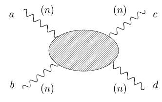
Figure 1: Elastic scattering of longitudinal modes of KK gauge bosons, $n+n\to n+n$, with the gauge index structure $a+b\to c+d$.

We want to calculate the energy dependence of the amplitude of the elastic scattering of the longitudinal modes of the KK gauge bosons $n+n\to n+n$ with gauge index structure $a+b\to c+d$ (see Fig. 1), where this process involves both exchange of the $k$’th KK mode from the cubic vertex, and the direct contribution from the quartic vertex. We will also assume, that the BC’s corresponding to the external modes with gauge indices $a,b,c,d$ are of the same type, that is they have the same KK towers (however we will not assume this for the modes that are being exchanged). There are four diagrams as shown in Fig. 2: the $s$, $t$ and $u$-channel exchange of the KK modes, and the contribution of the quartic vertex. The kinematics assumed for this elastic scattering is in the center of mass frame, where the incoming momentum vectors are $p_{\mu}=(E,0,0,\pm\sqrt{E^{2}-M_{n}^{2}})$, while the outgoing momenta are $(E,\pm\sqrt{E^{2}-M_{n}^{2}}\sin\theta,0,\pm\sqrt{E^{2}-M_{n}^{2}}\cos\theta)$. $E$ is the incoming energy, and $\theta$ the scattering angle with forward scattering for $\theta=0$. The longitudinal polarization vectors are as usual $\epsilon_{\mu}=(\frac{|\vec{p}|}{M},\frac{E}{M}\frac{\vec{p}}{|\vec{p}|})$ and accordingly the contribution of each diagram can be as bad as $E^{4}/M_{n}^{4}$. It is straightforward to evaluate the full scattering amplitude, and extract the leading behavior for large values energies of this amplitude. The general structure of the expansion in energy contains three terms:

$$\mathcal{A}=A^{(4)}\frac{E^{4}}{M_{n}^{4}}+A^{(2)}\frac{E^{2}}{M_{n}^{2}}+A^{(0)}+{\cal O}\left(\frac{M_{n}^{2}}{E^{2}}\right).$$ (3.1)

Figure 2: The four gauge diagrams contributing at tree level to the gauge boson elastic scattering amplitude.

It may seem inconsistent to formally expand the amplitude in energies, when for any fixed energy there are KK modes that are much heavier and the series is potentially non-convergent. However from the higher dimensional effective field theory we can see that the heaviest modes are not important. Summing over all the modes is just the simplest way of maintaining gauge invariance which would be broken by a hard cutoff on the spectrum.

To show this consider a non-Abelian gauge theory in $D$ dimensions with a cutoff $\Lambda$. The leading effect of integrating out the KK modes above $\Lambda$ should be given by gauge invariant higher dimensional operators. An example of such operators is given by

$$\frac{g_{D}^{3}}{\Lambda^{6-D}}F_{MN}^{3}~{}.$$ (3.2)

All other gauge invariant operators of the same dimension should give similar results for the scattering amplitudes. The coefficient of this operator can be fixed by first going into the normalization where the coefficient of the kinetic term is $-1/(4g_{D}^{2})$. In this normalization $F_{MN}$ has dimension two, thus the prefactor $1/\Lambda^{6-D}$. Going back to canonical normalization we get the higher order term of (3.2). Alternatively, we can see that this operator contains three gauge fields, so if it comes from a loop of massive gauge fields it should contain three gauge couplings. The contribution to longitudinal scattering from the ordinary $F_{MN}^{2}$ term is proportional to

$$g_{D}^{2}\left(ER\right)^{4}$$ (3.3)

(where we have assumed the incoming gauge boson mass is ${\cal O}(1/R)$, the inverse of the compactification radius). This can be seen easiest by looking at the four-point coupling of the gauge field. That has an explicit factor of $g_{D}^{2}$, and there are four polarization vectors which are of order $E/M\sim ER$. Naively, the contribution from the higher dimensional operator is growing faster with energy, with a power $E^{6}$. However, gauge invariance will actually soften this amplitude. One can see this explicitly by noting that from (3.2) one needs two factors of $\partial_{\mu}A_{\nu}-\partial_{\nu}A_{\mu}$, and two other factors of the gauge field. This will imply that two of the polarization vectors appear in the combination $p_{\mu}\epsilon_{\nu}-p_{\nu}\epsilon_{\mu}$, which after explicitly substituting for the polarization vectors is just proportional to the mass of the external particle, rather than growing with energy. Therefore the contribution from the $F_{MN}^{3}$ terms scales as

$$\frac{g_{D}^{4}}{\Lambda^{6-D}}\left(ER\right)^{2}\frac{1}{R^{2}}\,,$$ (3.4)

so the ratio of the correction term to the leading term is

$$\frac{g_{4}^{2}}{(\Lambda R)^{6-D}(ER)^{2}}\,,$$ (3.5)

where we have used $g_{D}^{2}=g_{4}^{2}R^{D-4}$. Thus for $E\gg 1/R$, $\Lambda R>1$, and $D<6$ the contributions from the highest KK modes are suppressed. Note that here we have not used the non-trivial cancellation of the $E^{4}$ term in the amplitude. Once that is taken into account, the effects of the KK modes are still suppressed as long as $D<6$ and $\Lambda R>1$. For a 5D theory $\Lambda R$ can be large as $24\pi^{3}$ [16].

We would like to understand under what circumstances $A^{(4)}$ and $A^{(2)}$ vanish. The vanishing of these coefficients would ensure that there are no terms in the amplitude that explicitly grow with energy. This is a necessary condition for the tree-level unitarity of a theory. However, this is certainly not a sufficient condition. The finite piece in the amplitude $A^{(0)}$ should also not be too large in order for the theory to be tree-unitary, for every possible scattering. In theories with extra dimensions, since there are an infinite number of KK modes available, there will always be some amplitudes that have finite pieces, which however grow as the number of exchanged KK modes is allowed to increase. This simply reflects the higher dimensional nature of the theory, and the fact that higher dimensional gauge theories are non-renormalizable. Therefore, tree unitarity is expected to break down at energies comparable to the 5D cutoff scale, even when $A^{(4)}=A^{(2)}=0.$ When discussing unitarity of these models we will simply mean the cancellation of the $A^{(4)}$ and $A^{(2)}$ amplitudes. We stress again that this does not imply that the conventional unitarity bounds on the finite amplitudes have to be satisfied for all processes.

The largest term, growing with $E^{4}$, depends only on the effective couplings and not on the mass spectrum:

$$A^{(4)}=i\left(g^{2}_{nnnn}-\sum_{k}g_{nnk}^{2}\right)\left(f^{abe}f^{cde}(3+6\cos\theta-\cos^{2}\theta)+2(3-\cos^{2}\theta)f^{ace}f^{bde}\right).$$ (3.6)

The expression for the amplitude that grows with $E^{2}$ is:

$$A^{(2)}=\frac{i}{M_{n}^{2}}f^{ace}f^{bde}\left(4g_{nnnn}^{2}M_{n}^{2}-3\sum_{k}g_{nnk}^{2}M_{k}^{2}\right)-\frac{i}{2M_{n}^{2}}f^{abe}f^{cde}\left(4g_{nnnn}^{2}M_{n}^{2}\vphantom{-3\sum_{k}M_{k}^{2}g_{nnk}^{2}}\right.$$

$$\left.-3\sum_{k}g_{nnk}^{2}M_{k}^{2}+\left(12g_{nnnn}^{2}M_{n}^{2}+\sum_{k}g_{nnk}^{2}(3M_{k}^{2}-16M_{n}^{2})\right)\cos\theta\right).$$ (3.7)

Both in (3.6) and (3.7) everywhere below the KK indices $n$ and $k$ actually have to be interpreted as double indices, that stand both for the color index and the KK number of the given color index, e.g., $k\sim(k,e)$. Also, as stated above, we are assuming that all the in-going and out-going gauge bosons satisfy the same boundary condition and thus the $n$ index is color-blind. In getting the expressions (3.7) or (3.9) for $A^{(2)}$, we used the Jacobi identity which requires a sum over the gauge index of the exchanged gauge boson. Thus we have implicitly assumed that the sums like $\sum_{k}g_{nnk}^{abe}g_{nnk}^{cde}$ or $\sum_{k}g_{nnk}^{abe}g_{nnk}^{cde}M_{k}^{e\,2}$ are independent of the gauge index $e$, which indeed is a true statement as we will show later on.

If one assumes the cancellation of the $E^{4}$ terms (which we will show is indeed always the case) one has the relation

$$g^{2}_{nnnn}=\sum_{k}g_{nnk}^{2}.$$ (3.8)

Using this relation the expression for the $E^{2}$ terms can be simplified to the following:

$$A^{(2)}=\frac{i}{M_{n}^{2}}\left(4g_{nnnn}M_{n}^{2}-3\sum_{k}g_{nnk}^{2}M_{k}^{2}\right)\left(f^{ace}f^{bde}-\sin^{2}{\textstyle\frac{\theta}{2}}\ f^{abe}f^{cde}\right).$$ (3.9)

Even though we will not consider constraints coming from the finite ($E^{0}$) terms in the elastic scattering amplitude, for completeness we present the relevant expression here (making use of the conditions for cancelling the $A^{(4)}$ and $A^{(2)}$ terms):

$$A^{(0)}=i\sum_{k}g_{nnk}^{2}\left(f^{abe}f^{cde}F(M_{k}/M_{n},\theta)+f^{ace}f^{bde}G(M_{k}/M_{n},\theta)\right),$$ (3.10)

with

$$F(x,\theta)=-\frac{1}{16\cos^{2}\theta/2}(4-10x^{2}+7x^{4}-8(4-3x^{2})\cos\theta-(4-2x^{2}-x^{4})\cos 2\theta),$$

$$G(x,\theta)=\frac{1}{2\sin^{2}\theta}(4-6x^{2}+3x^{4}+(12-10x^{2}+x^{4})\cos^{2}\theta).$$ (3.11)

We can summarize the above results by restating the conditions under which the terms that grow with energy cancel:

$$g^{2}_{nnnn} = \sum_{k}g_{nnk}^{2},$$ (3.12)

$$4g_{nnnn}^{2}M_{n}^{2} = 3\sum_{k}g_{nnk}^{2}M_{k}^{2}\,.$$ (3.13)

3.2 Cancellation of the terms that grow with energy for the simplest BC’s

The goal of the remainder of this section is to examine under what circumstances the terms that grow with energy cancel. Consider first the $E^{4}$ term. According to (3.12) the requirement for cancellation is

$$\int_{0}^{\pi R}dy\,f_{n}^{4}(y)=\sum_{k}\int_{0}^{\pi R}dy\int_{0}^{\pi R}dz\ f_{n}^{2}(y)f_{n}^{2}(z)f_{k}^{\vphantom{2}}(y)f_{k}^{\vphantom{2}}(z).$$ (3.14)

One can easily see that this equation is in fact satisfied no matter what BC one is imposing, as long as that BC still maintains hermiticity of the differential operator $\partial_{y}^{2}$ on $0,\pi R$. The BC maintains hermiticity of the differential operator if it is of the form ${f^{\prime}}_{|0,\pi R}=V_{0,\pi R}f_{|0,\pi R}$. In this case one can explicitly check that $\int_{0}^{\pi R}h^{*}{g^{\prime\prime}}=\int_{0}^{\pi R}{h^{*}}^{\prime\prime}g$. The reason why (3.14) is obeyed is that for such hermitian operators one is guaranteed to get an orthonormal complete set of solutions $f_{k}(y)$, thus from the completeness it follows that

$$\sum_{k}f_{k}(y)f_{k}(z)=\delta(y-z),$$ (3.15)

which immediately implies (3.14). The completeness relation basically implies that any function can be expanded in terms of the eigenfunctions of $\partial_{y}^{2}$ on the interval $0,\pi R$, $g(y)=\sum_{k}f_{k}(y)\int_{0}^{\pi R}dzg(z)f_{k}(z)$. There is a subtlety in this if the BC for the $f$’s is $f(0,\pi R)=0$, since in that case only functions that are themselves zero at the boundary can be expanded in this series. However, even in this case the expansion will converge everywhere except at the two endpoints to the given function, and since we will integrate over the interval anyway, changing the function at finite number of points does not matter. Thus we conclude that (3.14) always holds, the $E^{4}$ terms always cancel irrespectively of the BC’s imposed. Therefore, we can now assume that the $E^{4}$ terms cancelled, and using the equation that leads to the cancellation of these terms we get that the condition for the cancellation of the $E^{2}$ terms is as in (3.13)

$$3\,\sum_{k}M_{k}^{2}\int_{0}^{\pi R}dy\int_{0}^{\pi R}dz\,f_{n}^{2}(y)f_{n}^{2}(z)f_{k}^{\vphantom{2}}(y)f_{k}^{\vphantom{2}}(z)=4\,M_{n}^{2}\int_{0}^{\pi R}dy\,f_{n}^{4}(y).$$ (3.16)

Let us first assume that one can integrate by parts freely without picking up any boundary terms (we will later see under what circumstances this assumption is indeed justified). In this case we can easily derive a sum rule of the form

$$\sum_{k}M_{k}^{2p}\left(\int_{0}^{\pi R}dy\,f_{n}^{2}(y)f_{k}^{\vphantom{2}}(y)\right)^{2}=\frac{2^{2p}}{3}M_{n}^{2p}\int_{0}^{\pi R}dyf_{n}^{4}(y).$$ (3.17)

Indeed, let us define

$$a_{p}^{(k)}=M_{k}^{2p}\int_{0}^{\pi R}dy\,f_{n}^{2}(y)f_{k}^{\vphantom{2}}(y),\ \ b_{p}^{(k)}=M_{k}^{2p}\int_{0}^{\pi R}dy\,f^{\prime}_{n}{}^{2}(y)f_{k}^{\vphantom{2}}(y).$$ (3.18)

Using the 5D Lorentz invariant relation between the wavefunction and the mass spectrum, $M_{k}^{2}f_{k}(y)=-f_{k}^{\prime\prime}(y)$, a simple integration by part gives, neglecting the boundary terms that we will include in the next section, the recurrence relations:

$$a_{p+1}^{(k)}=2M_{n}^{2}a_{p}^{(k)}-2b_{p}^{(k)},\ \ b_{p+1}^{(k)}=2M_{n}^{2}b_{p}^{(k)}-2M_{n}^{4}a_{p}^{(k)},$$ (3.19)

from which we obtain that

$$a_{p}^{(k)}=2^{2p-1}M_{n}^{2p-2}\left(M_{n}^{2}a_{0}^{(k)}-b_{0}^{(k)}\right).$$ (3.20)

The completeness relation (3.15) finally allows to evaluate the sums:

$$\sum_{k}\big{(}a_{0}^{(k)}\big{)}^{2}=\int_{0}^{\pi R}dy\,f_{n}^{4}(y),\ \ \sum_{k}a_{0}^{(k)}b_{0}^{(k)}={\textstyle\frac{1}{3}}M_{n}^{2}\int_{0}^{\pi R}dy\,f_{n}^{4}(y),$$ (3.21)

which, combined with the recurrence relation, lead to the sum rule (3.17). For $p=1$ this relation exactly coincides with (3.16), and implies the cancellation of the $E^{2}$ terms.

3.3 Sum rule with boundary terms

In the previous section, we have derived, neglecting some possible boundary terms, a sum rule which ensures the cancellation of the terms that grow with the energy in the scattering amplitude. We now would like to keep track of those boundary terms and see under which circumstances the terms in the scattering amplitude that grow with energy still vanish. As discussed above, the cancellation of the $E^{4}$ terms is always ensured by the completeness of the eigenfunctions of $\partial_{y}^{2}$. However, the sum rule in (3.16) will be modified if there are non-vanishing boundary terms picked up when integrating by parts. The resulting corrections to the sum rule relevant for the $E^{2}$ term is given by (we denote again by $[F]$ the boundary quantity $F(\pi R)-F(0)$)

$$\sum_{k}\,M_{k}^{2}\ \left(\int dyf_{n}^{2}(y)f_{k}^{\vphantom{2}}(y)\right)^{2}={\textstyle\frac{4}{3}}M_{n}^{2}\int dyf_{n}^{4}(y)-{\textstyle\frac{2}{3}}[f_{n}^{3}f^{\prime}_{n}]\hphantom{spacespace}$$

$$-\sum_{k}\,[f_{n}^{2}f^{\prime}_{k}]\int dyf_{n}^{2}(y)f_{k}^{\vphantom{2}}(y)+2\sum_{k}\,[f_{n}^{\vphantom{2}}f^{\prime}_{n}f_{k}^{\vphantom{2}}]\int dyf_{n}^{2}(y)f_{k}^{\vphantom{2}}(y).$$ (3.22)

Thus one can see that (as expected) for arbitrary BC’s the $E^{2}$ terms no longer cancel. However, if one has pure Dirichlet or Neumann BC’s for all modes (some could have Dirichlet and some could have Neumann, but none should have a mixed boundary condition as in Eq. (2.16)) then all the extra boundary terms will vanish, and thus the cancellation of the $E^{2}$ terms would remain. Clearly, the terms in (3.22) involving $[f_{n}^{\vphantom{2}}f^{\prime}_{n}]$ vanish, since for the external mode either the function or its derivative should vanish on the boundary. The one term that needs to be analyzed more carefully is $\sum_{k}[f_{n}^{2}f^{\prime}_{k}]\int dyf_{n}^{2}(y)f_{k}(y)^{\vphantom{2}}$. If $f_{n}^{\vphantom{2}}$ satisfies Neumann BC’s, while $f_{k}$ Dirichlet, then the boundary piece itself is not vanishing. However, in this case the expansion in terms of $f_{k}$ converges even on the boundary, and thus $\sum_{k}f^{\prime}_{k}(x)\int f_{n}^{2}(y)f_{k}^{\vphantom{2}}(y)dy$ converges to $2f_{n}^{\vphantom{2}}(x)f^{\prime}_{n}(x)$, and thus we will again have a product $[f_{n}^{\vphantom{2}}f^{\prime}_{n}]$ on the boundaries, which will vanish.

Thus we can conclude that in theories with only Dirichlet or Neumann BC’s imposed the $E^{2}$ terms in the scattering amplitudes will always cancel. This implies, for example that all models that are obtained via an orbifolding procedure (that is taking an extra dimensional theory on a circle, and projecting onto modes that have a given property under $y\to-y$ and $\pi R-y\to\pi R+y$ projections) will be tree-unitary at least up to around the cutoff scale of the theory. In fact, we can see that for all consistent BC’s from (2.11) the $E^{2}$ terms vanish. This shows that, as expected, those BC’s which follow from a gauge invariant Lagrangian will have a proper high energy behavior. However, in the presence of mixed BC, the boundary terms in the piece of the scattering amplitude that grows with $E^{2}$ are non-vanishing and prevent the theory to be tree-unitarity up to the naive cutoff scale of the theory, e.g., the perturbative cutoff. The reason is that this corresponds to adding an explicit mass term for the gauge bosons on the boundary which violates gauge invariance. If however this comes from a gauge invariant scalar kinetic term via the Higgs mechanism, then extra scalar degrees of freedom need to be added. As we will see explicitly in the example of section 5.2, some extra degrees of freedom localized at the boundary are indeed needed to restore tree-unitarity in this case. In some limits, however, these extra localized states can decouple without spoiling tree-unitarity.

We close this section by presenting the corrections to the sum rule that is relevant for the evaluation of the $E^{0}$ terms of the scattering amplitude:

$$\sum_{k}\left(\int dyf_{n}^{2}f_{k}^{\vphantom{2}}\right)^{2}M_{k}^{4}={\textstyle\frac{16}{3}}M_{n}^{4}\int dyf_{n}^{4}+{\textstyle\frac{28}{3}}M_{n}^{2}[f_{n}^{3}f^{\prime}_{n}]-4[f_{n}^{\vphantom{2}}{f^{\prime}_{n}}^{3}]+\sum_{k}[f_{n}^{2}f^{\prime}_{k}-2f_{n}^{\vphantom{2}}f^{\prime}_{n}f_{k}^{\vphantom{2}}]^{2}$$

$$\vspace{-.5cm}-\sum_{k}\left(4M_{n}^{2}[f_{n}^{2}f^{\prime}_{k}]\int dyf_{n}^{2}f_{k}^{\vphantom{2}}-2[{f^{\prime}_{n}}^{2}f^{\prime}_{k}]\int dyf_{n}^{2}f_{k}^{\vphantom{2}}-2[f_{n}^{2}f^{\prime}_{k}]\int dy{f^{\prime}_{n}}^{2}f_{k}^{\vphantom{2}}\right).\ \$$ (3.23)

This is the relation that needs to be used if one were to try to find the actual unitarity bounds on the finite pieces of the elastic scattering amplitudes, which is beyond the scope of this paper.

4 A 4D Effective Theory Without a Higgs

We have seen above that the necessary conditions for cancelling the growing terms in the elastic scattering amplitudes are

$$g^{2}_{nnnn} = \sum_{k}g_{nnk}^{2},$$ (4.1)

$$4g_{nnnn}^{2}M_{n}^{2} = 3\sum_{k}g_{nnk}^{2}M_{k}^{2}\,.$$ (4.2)

One can ask the question, in what kind of low-energy effective theories could these conditions be possibly satisfied. Assuming, that there are $N$ gauge bosons, one can clearly always satisfy the relations (4.1)-(4.2) for the first $N-1$ particles, as long as $g_{nnnn}^{2}\geq g_{nnn}^{2}$. Given the couplings $g_{111}$ and $g_{1111}$ and the mass of the lightest gauge boson $M_{1}^{2}$, the necessary couplings and masses for the second gauge boson can be calculated from (4.1)-(4.2) to be

$$g_{112}^{2}=g_{1111}^{2}-g_{111}^{2},\ \ M_{2}^{2}=\frac{M_{1}^{2}}{g_{112}^{2}}\left(\frac{4}{3}g_{1111}^{2}-g_{111}^{2}\right),$$ (4.3)

assuming that a single extra gauge boson is needed to cancel the growing amplitudes. Clearly, there are many other possibilities as well to satisfy these equations for the $N-1$ lightest particles. However, the equation can not be satisfied for the heaviest mode itself. The reason is that for the heaviest particle one would get the equations

$$g_{NNNN}^{2}=\sum_{k}g_{NNk}^{2},\ \ \ g_{NNNN}^{2}=\sum_{k}g_{NNk}^{2}\,\frac{3M_{k}^{2}}{4M_{N}^{2}}.$$ (4.4)

Since the ratio $3M_{k}^{2}/(4M_{N}^{2})<1$ for the heaviest mode, these equations can not be solved no matter what the solution for the first $N-1$ particles was, as long as one has a finite number of modes. Thus we can see that there can not be a heaviest mode, for every gauge boson there needs to be one that is more heavy if one wants to ensure unitarity for all amplitudes. Thus a Kaluza-Klein type tower must be present by these considerations if the theory is to be fully unitary without any scalars, and (4.1)-(4.2) can be satisfied only in the presence of infinitely many gauge bosons.

From an effective theory point of view one should however consider the theory with a cutoff scale. Then there would be a finite number of modes below this cutoff scale, for all of which one could ensure the unitarity relations, except for the mode closest to the cutoff, for which one has to assume that the UV completion plays a role in unitarizing the amplitude. However, from this point of view we can see that the cutoff scale could be much higher than the one naively estimated from the growing $E^{2}$ amplitudes within the standard model. For example, in the minimal case a single $W^{\prime}$ and $Z^{\prime}$ gauge bosons are necessary to unitarize the $W_{L}^{+}W_{L}^{-}$ and $Z_{L}Z_{L}$ scattering amplitudes. In fact, the relations (4.1)-(4.2) can be satisfied with a $W^{\prime}$ and $Z^{\prime}$ that are heavy enough and sufficiently weakly coupled, so that their effects would not have been observed at the Tevatron nor would they have significantly contributed to electroweak precision observables.

For example, in the SM the scattering $W_{L}^{+}W_{L}^{-}\to W_{L}^{+}W_{L}^{-}$ is mediated by $s$, $t$ and $u$-channel $Z$ and $\gamma$ exchange, and by the direct quartic coupling. The cancellation of the $E^{4}$ term in the SM is ensured by the relations

$$g^{2}_{WWWW}=g^{2},\ \ \ g^{2}_{WWZ}=g^{2}\cos^{2}\theta_{W},\ \ \ g^{2}_{WW\gamma}=e^{2}=g^{2}\sin^{2}\theta_{W}.$$ (4.5)

Let us now assume that the relation between $g^{2}_{WWWW}$ and $g^{2}_{WWZ}$ is slightly modified due to the existence of a heavy $Z^{\prime}$, which has a small cubic coupling with the $W$’s $g^{2}_{WWZ^{\prime}}$. The values of the three gauge boson couplings $g_{WWZ}$ and $g_{WW\gamma}$ are not strongly constrained by experiments, they are known to coincide with the SM values to a precision of about 3-5% , while there is basically no existing experimental constraint on $g^{2}_{WWWW}$. Let us therefore assume that the three gauge boson coupling $g^{2}_{WWZ}$ is smaller by a percent than the SM prediction. Then in order to maintain the cancellation of the $E^{4}$ terms one needs $g^{2}_{WWZ^{\prime}}\sim 0.01g^{2}_{WWZ}$. The cancellation of the $E^{2}$ terms would then fix the mass of the $Z^{\prime}$ to be about $560$ GeV.

Note that one would not expect a quartic $Z$ coupling or a $ZZ\gamma$ coupling, since there is none in the SM, thus there are no contributions to $Z_{L}Z_{L}\to Z_{L}Z_{L}$ (contrary to the SM where the Higgs exchange provides a finite term). However, to unitarize the $W_{L}Z_{L}\to W_{L}Z_{L}$ amplitude there also needs to be a heavy $W^{\prime}$, with couplings to $W$ and $Z$ $g^{2}_{WZW^{\prime}}$ similar to $g^{2}_{WWZ^{\prime}}$. Thus (without actually having calculated the coefficients of the amplitudes for the inelastic scatterings) we expect that $W^{\prime}$ would also have a mass of order 500 GeV. This way all the amplitudes involving only SM $W$’s and $Z$’s in initial and final states would be unitarized. However, due to the sum rule explained above the scattering amplitudes involving the $W^{\prime}$ and $Z^{\prime}$ in initial and final states can not all be cancelled by only these particles. We expect that these amplitudes would become large at scales that are set by the masses of the $W^{\prime}$ and $Z^{\prime}$ rather than the ordinary $W$ and $Z$, so this would roughly correspond to a scale of order $4\pi M_{W^{\prime}}/g\sim 10$ TeV, were the theory with only these particles would break down.

Since the 4D effective theory below $\Lambda=10$ TeV does not have an $SU(2)_{L}$ gauge invariance (not even a hidden gauge invariance) there is an issue with the mass renormalization for the gauge bosons: there will be quadratic divergences in the $W$ and $Z$ mass. (If the theory is completed into an extra dimensional gauge theory with gauge symmetry breaking by boundary conditions, then the masses will not really be quadratcially divergent, the divergences will be cut off roughly by the radius of the extra dimension.) However the theory is still technically natural since there is a limit where (hidden) gauge invariance is restored and the divergence must be proportional to the gauge invariance breaking spurion. In the present example we can estimate the divergent contribution to the $Z$ mass to be at most

$$\delta M_{Z}^{2}\approx 0.01\frac{g^{2}_{WWZ}}{16\pi^{2}}\Lambda^{2}\approx 0.7\,{\rm GeV}^{2}~{}.$$ (4.6)

The three gauge boson couplings required between the heavy and the light gauge bosons is quite small. Therefore loop contributions to the oblique parameters $S,T,U$ will be strongly suppressed. However, one has to still ensure that no large tree-level effects appear due to mixings between the heavy and light gauge bosons, which could spoil electroweak precision observables. In practice, this will probably require that the interactions of the heavy $W^{\prime}$ and $Z^{\prime}$ obey a global SU(2)_C custodial symmetry which ensures $\rho=1$ in the SM

The masses of order 500 GeV would fall to the borderline region of direct observation, assuming that their couplings to fermions is equal to the SM couplings. However, if the coupling to fermions is just slightly suppressed, or it decays dominantly to quarks or through cascades, then the direct search bounds could be easily evaded.

One should ask what kind of theories would actually yield low-energy effective theories of the sort discussed in this section. We will see below that some extra dimensional models could come quite close, though the masses of the gauge bosons are lower than 500 GeV, while the $\rho$ parameter has to be tuned to its experimental value. Before moving on to these models, let us discuss whether any 4D theories with product group structure could result in cancellations of the growing amplitudes. These models would correspond to deconstructed extra dimensional theories. It has been shown in [18] that for finite number $N$ of product gauge groups there will be leftover pieces in the $E^{2}$ amplitude (without including Higgs exchange) that scale with $N$ like $1/N^{3}$ (see Appendix B for details). Therefore, in any linear or non-linear realizations of product groups broken by mass terms on the link fields the amplitudes will not be unitary. However, already for $N=3$ one would get a suppression factor of 27 in the $E^{2}$ piece of the scattering amplitude, which would mean that the scale at which unitarity violations would become visible would be of order 8 TeV, rather than the usual 1.5 TeV scale. Below we will focus on the models based on extra dimensions, where the cancellation of the $E^{2}$ terms is automatic without a scalar exchange.

5 Examples of Unitarity in Higher Dimensional Theories

In this section we will present two examples of how the unitarity relations (3.12)-(3.13) are satisfied in particular extra dimensional theories. The first example will be based on pure Dirichlet or Neumann boundary conditions, where the cancellation as expected is automatic, while the second example will involve mixed BC’s for some of the gauge bosons, which will imply the non-cancellation of the $E^{2}$ terms. However, as we will show unitarity can be restored by introducing a boundary Higgs field.

5.1 SU(2)$\to$ U(1) by BC

Let us consider a 5D $SU(2)$ Yang–Mills theory compactified on an orbifold that leaves only a $U(1)$ subgroup unbroken. We will further impose a Scherk–Schwarz periodic condition in order to project out all the 4D scalar fields coming from the component of the gauge fields along the extra dimension. The 5D gauge fields thus satisfy:

$$A_{\mu}(x,-y)=PA_{\mu}(x,y)P^{-1}\ \ \ {\rm and} \ \ \ A_{5}(x,-y)=-PA_{5}(x,y)P^{-1},$$ (5.1)

$$A_{\mu}(x,y+2\pi R)=TA_{\mu}(x,y)T^{-1}\ \ \ {\rm and} \ \ \ A_{5}(x,y+2\pi R)=TA_{5}(x,y)T^{-1}.$$ (5.2)

where $A_{M}=A_{M}^{a}\tau^{a}/2$ ($\tau^{a},a=1\ldots 3$ are the Pauli matrices) is the gauge field and $P=\rm{diag}(1,-1)$, the orbifold projection and $T=P$, the Scherk–Schwarz shift. Note that the orbifold projection and the Scherk–Schwarz shift satisfy the consistency relation [19]: $PTP=T^{-1}$. This setup could alternatively also be described by two $Z_{2}$ projections $y\to-y$ and $\pi R-y\to\pi R+y$. The action of the first $Z$ is just as in (5.1), while the second one is similar with $P$ replaced by $PT=P^{2}=1$.

Equivalently, we can describe this orbifold by a finite interval ($y\in[0,\pi R]$) supplemented by the BC’s:

$$A^{1,2}_{\mu}(x,0)=0,\partial_{5}A^{3}_{\mu}(x,0)=0,\partial_{5}A^{a}_{\mu}(x,\pi R)=0$$ (5.3)

$$\partial_{5}A^{1,2}_{5}(x,0)=0,A^{3}_{5}(x,0)=0,A^{a}_{5}(x,\pi R)=0$$ (5.4)

Note that there is no zero mode coming from the fifth components of the gauge fields. Therefore, we go to the unitary gauge which is the same as the axial gauge ($A_{5}=0$). Then the KK decomposition is

$$\displaystyle A^{1}_{\mu}(x,y)=\sum_{k=0}^{\infty}\frac{1}{\sqrt{\pi R}}\sin\left(\frac{(2k+1)y}{2R}\right)(W^{+\,(k)}_{\mu}(x)+W^{-\,(k)}_{\mu}(x)),$$ (5.5)

$$\displaystyle A^{2}_{\mu}(x,y)=\sum_{k=0}^{\infty}\frac{i}{\sqrt{\pi R}}\sin\left(\frac{(2k+1)y}{2R}\right)(W^{+\,(k)}_{\mu}(x)-W^{-\,(k)}_{\mu}(x)),$$ (5.6)

$$\displaystyle A^{3}_{\mu}(x,y)=\sum_{k=0}^{\infty}\sqrt{\frac{2}{2^{\delta_{k,0}}\pi R}}\cos\left(\frac{ky}{R}\right)\gamma^{(k)}_{\mu}(x).$$ (5.7)

The spectrum contains a massless photon, $\gamma^{(0)}$, and its KK excitations, $\gamma^{(k)}$, of mass $M_{\gamma^{(k)}}=k/R$ as well as a tower of massive charged gauge bosons, $W^{\pm\,(k)}$, of mass $M_{W^{(k)}}=(2k+1)/(2R)$. With the above wavefunctions, it is easy to explicitly compute the cubic and quartic effective couplings and check the general sum rules of Section 2. For instance, for the elastic scattering of $W$’s, the relevant couplings are:

$$\displaystyle g_{W^{(n)}W^{(n)}\gamma^{(k)}}=\frac{g_{5}}{2\sqrt{\pi R}}\left(\delta_{k,0}-\frac{1}{\sqrt{2}}\delta_{k,2n+1}\right),$$ (5.8)

$$\displaystyle g^{2}_{W^{(n)}W^{(n)}W^{(n)}W^{(n)}}=\frac{3g_{5}^{2}}{8\pi R}.$$ (5.9)

The BC’s conserve KK momenta up to a sign and therefore only $\gamma^{(0)}$ and $\gamma^{(2n+1)}$ can contribute to the elastic scattering of $W^{(n)}$’s. The sum rules (3.12)–(3.13) are trivially fulfilled.

The point of this section was to show that it is indeed possible to give a mass to gauge boson without relying on a Higgs mechanism to restore unitarity. The orbifold symmetry breaking mechanism illustrated with this example is however restrictive since it uses a $Z_{2}$ symmetry of the action and in the simplest cases (abelian orbifolds using an inner automorphism) it is even impossible to reduce the rank the gauge group, which is a serious obstacle to the construction of realistic phenomenological models. There are, however, more general BC’s we can impose that are not equivalent to a simple orbifold compactification but still lead to a well behaved effective theory.

5.2 Completely broken SU(2) by mixed BC’s and the need for a boundary Higgs field

In the previous section, we considered a breaking of $SU(2)$ down to $U(1)$ by an orbifold compactification. We have shown that, in agreement with our general proof of Section 2, the scattering amplitude of the gauge bosons that acquire a mass through compactification has a good high energy behavior. The cancellation of the terms growing with energy is ensured by the exchange of higher massive gauge bosons and does not require the presence of any scalar field. We would like now to consider some more general boundary conditions than the ones coming from orbifold compactification. In this case, we will see that the boundary terms of the sum rule (3.22) are non vanishing and thus lead to a violation of the unitarity at tree level, however unitarity can be restored by a scalar field living at the boundary. We illustrate these results with an example of an $SU(2)$ completely broken by mixed (neither Dirichlet nor Neumann) BC’s.

Let us thus now consider the BC’s:

$$\partial_{5}A^{a}_{\mu}(x,0)=0,\ \ \ \partial_{5}A^{a}_{\mu}(x,\pi R)=VA^{a}_{\mu}(x,\pi R),$$ (5.10)

$$A^{a}_{5}(x,0)=0,\ \ \ A^{a}_{5}(x,\pi R)=0.$$ (5.11)

A general solution can be decomposed on the KK basis

$$A^{a}_{\mu}(x,y)=\sum_{k=1}^{\infty}f_{k}(y)A^{(k)}_{\mu}(x),\ \ {\rm with}\ f_{k}(y)=\frac{a_{k}}{\sin(M_{k}\pi R)}\cos(M_{k}y).$$ (5.12)

The BC at the origin, $y=0$, is trivially satisfied while the condition at $y=\pi R$ determines the mass spectrum through the transcendental equation:

$$M_{k}\tan(M_{k}\pi R)=-V.$$ (5.13)

The parameter $V$ controls the gauge symmetry breaking: when $V=0$, the BC’s are those of a orbifold compactification with no symmetry breaking and when $V$ is turned on there is no zero mode any more and the full $SU(2)$ gauge group is broken completely. Note that there is no zero mode either for the fifth component of the gauge field and thus $A_{5}$ can be gauged away, leaving no scalar field in the low energy 4D effective theory.

The normalization factor $a_{k}$ is determined by requiring that the KK modes are canonically normalized, $\int_{0}^{\pi R}f_{k}^{2}(y)=1$, leading to

$$a_{k}=\frac{\sqrt{2}}{\sqrt{\pi R(1+M_{k}^{2}/V^{2})-1/V}}.$$ (5.14)

Note that this KK decomposition can equivalently be obtained through a much more lengthy procedure consisting in two steps (see [17] for details): (i) assume $V=0$, get a KK decomposition as in (5.7) and obtain the corresponding effective action; (ii) reintroduce the parameter $V$ in the effective action as a mass term that mixes all the previous modes and the true eigenmodes are obtained by diagonalizing the corresponding infinite mass matrix.

Unlike in the case of the previous section involving only Dirichlet or Neumann BC’s, the mixed BC’s (5.10) give rise to boundary terms in the sum rule (3.22) needed for the computation of the scattering amplitude. We obtain:

$$\sum_{k}\,M_{k}^{2}\ \left(\int dyf_{n}^{2}f_{k}^{\vphantom{2}}\right)^{2}={\textstyle\frac{4}{3}}M_{n}^{2}\int dyf_{n}^{4}+{\textstyle\frac{1}{3}}Vf_{n}^{4}(\pi R).$$ (5.15)

Consequently, the scattering amplitude has a residual piece growing with the energy square which is proportional to the order parameter, $V$:

$$A^{(2)}=\frac{ig_{5}^{2}}{M_{n}^{2}}Vf_{n}^{4}(\pi R)\left(-\delta^{ab}\delta^{cd}+\delta^{ac}\delta^{bd}\,\sin^{2}\theta/2+\delta^{ad}\delta^{bc}\,\cos^{2}\theta/2\right).$$ (5.16)

Besides the case $V=0$, there is another limit where these boundary terms actually vanish. Indeed, when $V\gg 1/R$, the low-lying eigenmasses can be approximated by

$$M_{k}\sim\frac{2k+1}{2R}\left(1+\frac{1}{\pi RV}+\ldots\right),\ \ k=0,1,2\ldots$$ (5.17)

and the normalization factor is $a_{k}\sim 1/\sqrt{\pi R}$, thus

$$Vf_{n}^{4}(\pi R)\sim\frac{(2n+1)^{4}}{4\pi^{2}R^{6}V^{3}}.$$ (5.18)

Therefore, the terms in the scattering amplitude that grow with the energy do cancel when $V$ goes to infinity. The physical reason of such a cancellation is clear: in the large $V$ limit, the brane localized mass term becomes large and the wavefunctions are expelled from the brane thus the mixed BC $\partial_{5}f_{k}(\pi R)=Vf_{k}(\pi R)$ in the limit $V\to\infty$ simply becomes equivalent to the Dirichlet BC $f_{k}(\pi R)=0$ which, as we already know, does not lead to any unitarity violation.

Figure 3: Higgs exchange contributing at tree level to the gauge boson elastic scattering amplitude. The Higgs boson is localized at $y=\pi R$ and the vertex Higgs-Gauge-Gauge is proportional to $f_{n}^{2}(\pi R)$.

As we already said, a finite and non-vanishing order parameter $V$ can be interpreted as an explicit gauge boson mass term localized at the boundary. This explicit breaking can be UV completed using the usual Higgs mechanism. In our $SU(2)$ model, we can introduce a 4D $SU(2)$ doublet localized at $y=\pi R$. Giving a vacuum expectation value to the lower component of the localized Higgs doublet

$$\langle H\rangle=\frac{1}{\sqrt{2}}\left(\begin{array}[]{c}0\\ v\end{array}\right)$$ (5.19)

gives rise to the mass term $\int d^{4}x{\textstyle\frac{1}{8}}g_{5}^{2}v^{2}A_{\mu}^{2}(x,\pi R)$ in the 5D action. To obtain the BC (see Appendix A.2 for technical details) we need to vary the action that contains both a bulk and a boundary piece. The relevant part of the action is

$$\left(\int_{0}^{\pi R}dy\,{\textstyle\frac{1}{2}}\partial_{5}A_{\mu}\partial_{5}A^{\mu}\right)+{\textstyle\frac{1}{8}}g_{5}^{2}v^{2}A^{2}_{\mu\,|\pi R}.$$ (5.20)

Varying the bulk terms will introduce, after integration by parts, the usual equation of motion as well as boundary terms:

$$-\left(\int_{0}^{\pi R}dy\,\partial_{5}^{2}A_{\mu}\,\delta A^{\mu}\right)+\left(\partial_{5}A_{\mu}\,\delta A^{\mu}+{\textstyle\frac{1}{4}}g_{5}^{2}v^{2}A_{\mu}\,\delta A^{\mu}\right)_{|\pi R}~{}.$$ (5.21)

The boundary terms thus impose the mixed BC:

$$\partial_{5}A_{\mu}^{a}(x,\pi R)=VA_{\mu}^{a}(x,\pi R),\ \ {\rm with}\ \ V=-{\textstyle\frac{1}{4}}g_{5}^{2}v^{2}.$$ (5.22)

The three Goldstone bosons are eaten by the KK gauge bosons that would be massless when $V=0$ and we are left with only one physical real scalar field, the Higgs boson. At tree level, the exchange of this Higgs boson also contributes to the gauge boson scattering amplitude through the diagrams depicted in Fig. 3. The Higgs being localized at $y=\pi R$, its coupling to the gauge bosons is proportional to $f_{k}^{2}(\pi R)$. Thus we get a contribution to the scattering amplitude that grows with the energy square:

$$A^{(2)}=\frac{ig_{5}^{4}v^{2}}{4M_{n}^{2}}f_{n}^{4}(\pi R)\left(-\delta^{ab}\delta^{cd}+\delta^{ac}\delta^{bd}\,\sin^{2}\theta/2+\delta^{ad}\delta^{bc}\,cos^{2}\theta/2\right).$$ (5.23)

Using the relation (5.22), we get that (as expected) the Higgs exchange exactly cancels the terms in scattering amplitude from the gauge exchange that grows like $E^{2}$. Remarkably enough, the Higgs boson can be decoupled ($v\to\infty$ limit) without spoiling the high energy behavior of the massive gauge boson scattering. Note, that this limit would simply correspond to the $A_{\mu}^{a}=0$ BC from (2.11).

6 A Toy Model for Electroweak Symmetry Breaking via BC’s

We want to study in this section the possibility to break the electroweak symmetry $SU(2)_{L}\times U(1)_{Y}$ down to $U(1)_{Q}$ along the lines of the previous section, i.e., by BC’s without relying on a Higgs mechanism either in the bulk or on the brane (a realistic model of electroweak symmetry breaking without any fundamental scalar field has been constructed in [21], see also [22]. Here we want to go further and totally remove any 4D scalar fields). The first idea would be to extend the analysis of Section 5.2 to include a mixing between $SU(2)$ and $U(1)$. However, considering the limit $V\to\infty$, we would get a mass degeneracy for the $W^{\pm}$ and the $Z$ gauge bosons. Our point is to show that we can actually lift this degeneracy and obtain a spectrum that depends on the gauge couplings. We do not claim to have a fully realistic model but we want to construct a toy model that has the characteristics of the Standard Model without the Higgs and that remains theoretically consistent.

Let us consider $SO(4)\times U(1)\sim SU(2)_{L}\times SU(2)_{R}\times U(1)$ compactified on an interval $[0,\pi R]$ (for other models using a left-right symmetric extra dimensional bulk see [23], thought the breaking patter of symmetries is very different in those models). At one end, we break $SO(4)$ down to $SU(2)_{D}$ by Neumann and Dirichlet BC’s. At the other end of the interval, we break $SU(2)_{R}\times U(1)$ down to $U(1)_{Y}$ by mixed BC’s and we will consider the limit $V\to\infty$ in order to ensure unitarity without having to introduce extra scalar degrees of freedom (alternatively, one can directly impose the equivalent Dirichlet BC’s, however, the gauge structure is more transparent using the limit of mixed BC’s). Thus only $U(1)_{Q}$ remains unbroken. We denote by $A^{R\,a}_{M}$, $A^{L\,a}_{M}$ and $B_{M}$ the gauge bosons of $SU(2)_{R}$, $SU(2)_{L}$ and $U(1)$ respectively; $g$ is the gauge coupling of the two $SU(2)$’s and ${g^{\prime}}$, the gauge coupling of the $U(1)$. We consider the two linear combinations of the $SU(2)$ gauge bosons $A^{\pm\,a}_{M}={\textstyle\frac{1}{\sqrt{2}}}(A^{L\,a}_{M}\pm A^{R\,a}_{M})$. We impose the following BC’s:

$${\rm at}\ y=0: \left\{\begin{array}[]{l}\partial_{5}A^{+\,a}_{\mu}=0,\ A^{-\,a}_{\mu}=0,\ \partial_{5}B_{\mu}=0,\\ \vrule height=15.0pt,depth=5.0pt,width=0.0ptA^{+\,a}_{5}=0,\ \partial_{5}A^{-\,a}_{5}=0,\ B_{5}=0.\end{array}\right.$$ (6.3)

$${\rm at}\ y=\pi R: \left\{\begin{array}[]{l}\partial_{5}A^{L\,a}_{\mu}=0,\ \partial_{5}A^{R\,1,2}_{\mu}=-{\textstyle\frac{1}{4}}g^{2}v^{2}A^{R\,1,2}_{\mu},\\ \vrule height=15.0pt,depth=5.0pt,width=0.0pt\partial_{5}B_{\mu}=-{\textstyle\frac{1}{4}}{g^{\prime}}v^{2}({g^{\prime}}B_{\mu}-gA^{R\,3}_{\mu}),\ \partial_{5}A^{R\,3}_{\mu}={\textstyle\frac{1}{4}}gv^{2}({g^{\prime}}B_{\mu}-gA^{R\,3}_{\mu}),\\ \vrule height=15.0pt,depth=5.0pt,width=0.0ptA^{L\,a}_{5}=0,\ A^{R\,a}_{5}=0,\ B_{5}=0.\end{array}\right.$$ (6.7)

One has to check now, that the equations (2.11) are indeed satisfied requiring these BC’s. We will only explain how the first of (2.11) is satisfied at $y=0$, one can similarly check all the other conditions. From $A^{-\,a}_{\mu}=0$ we get that $\delta A^{La}_{\mu}=\delta A^{Ra}_{\mu}$. Thus we need to show that $F^{La}_{\nu 5}+F^{Ra}_{\nu 5}=0$, which is true due to the requirements $\partial_{5}A^{+\,a}_{\mu}=0$, $A_{\mu}^{-\,a}=0$, and $A^{+\,a}_{5}=0$. Note, that these BC’s are a non-trivial example of (2.11) being satisfied without a term-by-term cancellation of the actual boundary variations, but rather by a cancellation among the various terms.

One may wonder where these complicated looking BC’s originate from. In fact, they correspond to a physical situation where one has an orbifold projection based on an outer automorphism $SU(2)_{L}\leftrightarrow SU(2)_{R}$ around one of the fixed points. Indeed the BC’s can be seen as deriving from the orbifold projections ($\hat{y}=y+\pi R$):

$$A^{L\,a}_{\mu}(x,-y)=A^{R\,a}_{\mu}(x,y)\,,\ A^{R\,a}_{\mu}(x,-y)=A^{L\,a}_{\mu}(x,y)\,,\ B_{\mu}(x,-y)=B_{\mu}(x,y)\ ,$$ (6.8)

$$A^{L\,a}_{\mu}(x,-\hat{y})=A^{L\,a}_{\mu}(x,\hat{y})\,,\ A^{R\,a}_{\mu}(x,-\hat{y})=A^{R\,a}_{\mu}(x,\hat{y})\,,\ B_{\mu}(x,-\hat{y})=B_{\mu}(x,\hat{y})\ .$$ (6.9)

The projections on the fifth components of the gauge fields are the same except an additional factor $-1$. At the $y=\pi R$ end point, a localized $SU(2)_{R}$ scalar doublet of $U(1)$ charge $1/2$ acquires a VEV $(0,v)/\sqrt{2}$ and breaks $SU(2)_{R}\times U(1)$ down to $U(1)_{Y}$. The mass terms is responsible for the mixed BC’s (6.7).

For a finite VEV, the 4D Higgs scalar localized at $y=\pi R$ is needed to keep the theory unitary; we will however consider the limit $v\to\infty$ where this scalar field can be decoupled without spoiling the high energy behavior of the gauge boson scattering.

Due to the mixing of the various gauge groups, the KK decomposition is more involved than in the simple example of Section 5.2 but it is obtained by simply enforcing the BC’s (we denote by $A^{L,R\,\pm}_{\mu}$ the linear combinations ${\textstyle\frac{1}{\sqrt{2}}}(A^{L,R\,1}\mp iA^{L,R\,2})$):

$$B_{\mu}(x,y) = g\,a_{0}\gamma_{\mu}(x)+{g^{\prime}}\sum_{k=1}^{\infty}b_{k}\cos(M^{Z}_{k}y)\,Z^{(k)}_{\mu}(x)\,,$$ (6.10)

$$A^{L\,3}_{\mu}(x,y) = {g^{\prime}}\,a_{0}\gamma_{\mu}(x)-g\sum_{k=1}^{\infty}b_{k}\frac{\cos(M^{Z}_{k}(y-\pi R))}{2\cos(M^{Z}_{k}\pi R)}\,Z^{(k)}_{\mu}(x)\,,$$ (6.11)

$$A^{R\,3}_{\mu}(x,y) = {g^{\prime}}a_{0}\gamma_{\mu}(x)-g\sum_{k=1}^{\infty}b_{k}\frac{\cos(M^{Z}_{k}(y+\pi R))}{2\cos(M^{Z}_{k}\pi R)}\,Z^{(k)}_{\mu}(x)\,,$$ (6.12)

$$A^{L\,\pm}_{\mu}(x,y) = \sum_{k=1}^{\infty}c_{k}\cos(M^{W}_{k}(y-\pi R))\,W^{(k)\,\pm}_{\mu}(x)\,,$$ (6.13)

$$A^{R\,\pm}_{\mu}(x,y) = \sum_{k=1}^{\infty}c_{k}\cos(M^{W}_{k}(y+\pi R))\,W^{(k)\,\pm}_{\mu}(x)\,.$$ (6.14)

The normalization factors, in the large VEV limit, are given by

$$a_{0}=\frac{1}{\sqrt{\pi R}}\frac{1}{\sqrt{g^{2}+2{g^{\prime}}^{2}}}\,,\ b_{k}\sim\frac{\sqrt{2}}{\sqrt{\pi R}}\frac{1}{\sqrt{g^{2}+2{g^{\prime}}^{2}}}\,,\ c_{k}\sim\frac{1}{\sqrt{\pi R}}\,.$$ (6.15)

The spectrum is made up of a massless photon, the gauge boson associated with the unbroken $U(1)_{Q}$ symmetry, and some towers of massive charged and neutral gauge bosons, $W^{(k)}$ and $Z^{(k)}$ respectively. The masses of the $W^{\pm}$’s are solution of

$$M^{W}_{k}\tan(2M^{W}_{k}\pi R)={\textstyle\frac{1}{4}}g^{2}v^{2}\,,$$ (6.16)

and in the large $v$ limit, we get the approximate spectrum:

$$M^{W}_{k}=\frac{2k-1}{4R}\left(1-\frac{2}{\pi g^{2}v^{2}R}+\ldots\right),\ \ k=1,2\ldots$$ (6.17)

The masses of the $Z$’s are solution of

$$M^{Z}_{k}\tan(M^{Z}_{k}\pi R)={\textstyle\frac{1}{8}}(g^{2}+2{{g^{\prime}}}^{2})v^{2}-{\textstyle\frac{1}{8}}g^{2}v^{2}\tan^{2}(M^{Z}_{k}\pi R)\,,$$ (6.18)

and in the large $v$ limit, we get two towers of neutral gauge bosons:

$$M^{Z}_{k}=\left(M_{0}+\frac{k-1}{R}\right)\left(1-\frac{2}{(g^{2}+{{g^{\prime}}}^{2})v^{2}\pi R}+\ldots\right),\ \ k=1,2\ldots$$ (6.19)

$$M^{Z^{\prime}}_{k}=\left(-M_{0}+\frac{k}{R}\right)\left(1-\frac{2}{(g^{2}+{{g^{\prime}}}^{2})v^{2}\pi R}+\ldots\right),\ \ k=1,2\ldots$$ (6.20)

where $M_{0}={\textstyle\frac{1}{\pi R}}\arctan\sqrt{1+2{{g^{\prime}}}^{2}/g^{2}}$. Note that $1/(4R)<M_{0}<1/(2R)$ and thus the $Z^{\prime}$’s are heavier than the $Z$’s ($M^{Z^{\prime}}_{k}>M^{Z}_{k}$). We also get that the lightest $Z$ is heavier than the lightest $W$ ($M^{Z}_{1}>M^{W}_{1}$), in agreement with the SM spectrum.

The BC’s break KK momentum conservation and as a consequence all the KK will interact to each other. For instance, the cubic effective couplings between the $W$’s and the $Z$’s (and the $Z^{\prime}$’s) are, in the large VEV limit,

$$g_{W^{(n)}W^{(n)}Z^{(k)}}=-\frac{2g^{2}}{\sqrt{\pi^{3}R^{3}(g^{2}+g^{\prime\,2})}}\frac{M_{n}^{W\,2}}{(4M^{W\,2}_{n}-M^{Z\,2}_{k})M^{Z}_{k}}\,,$$ (6.21)

while the couplings between the $W$’s and the photon are

$$g_{W^{(n)}W^{(n)}\gamma}=\frac{g{g^{\prime}}}{\sqrt{g^{2}+2{g^{\prime}}^{2}}}\frac{1}{\sqrt{\pi R}}\,.$$ (6.22)

Let us now discuss how to introduce matter fields. Locally at the $y=0$ boundary, a $SU(2)_{D}\times U(1)$ subgroup remains unbroken. We can introduce some matter fields localized on this boundary. Consider a $SU(2)$ scalar doublet with a $U(1)$ charge $\sqrt{2}q$. Its interactions with the gauge boson KK modes are generated through the localized covariant derivative

$$D_{\mu}\Phi=\partial_{\mu}\Phi-\frac{i}{2}\left(\begin{array}[]{cc}2\sqrt{2}{g^{\prime}}qB_{\mu}+gA^{+\,3}_{\mu}&g(A^{+\,1}_{\mu}-iA^{+\,2}_{\mu})\\ g(A^{+\,1}_{\mu}+iA^{+\,2}_{\mu})&2\sqrt{2}{g^{\prime}}qB_{\mu}-gA^{+\,3}_{\mu}\end{array}\right)_{|0}\Phi.$$ (6.23)

Using the KK decomposition (6.10)-(6.14), we evaluate the value of the gauge fields at the boundary and the scalar covariant derivative becomes

$$D_{\mu}\Phi=\partial_{\mu}\Phi - i\sqrt{2}g{g^{\prime}}a_{0}\left(\begin{array}[]{cc}q+{\textstyle\frac{1}{2}}&0\\ 0&q-{\textstyle\frac{1}{2}}\end{array}\right)\gamma_{\mu}\Phi-\sum_{k=1}^{\infty}\frac{ib_{k}g^{2}}{\sqrt{8}}\left(\begin{array}[]{cc}{\textstyle\frac{4q{g^{\prime}}^{2}}{g^{2}}}-1&0\\ 0&{\textstyle\frac{4q{g^{\prime}}^{2}}{g^{2}}}+1\end{array}\right)Z^{(k)}_{\mu}\Phi$$ (6.28)

$$- \sum_{k=1}^{\infty}igc_{k}\cos(M^{W}_{k}\pi R)\left(\begin{array}[]{cc}0&W^{(k)\,+}_{\mu}\\ W^{(k)\,-}_{\mu}&0\end{array}\right)\Phi.$$ (6.31)

The interactions between the scalar doublet $\Phi$ and the first massive KK gauge bosons $Z^{(1)}$ and $W^{(1)}$ will exactly reproduce the SM interactions between a $SU(2)_{L}$ doublet of hypercharge $q$ and the $Z$ and the $W$’s provided that the normalization factors $a,b_{1},c_{1}$ satisfy

$$b_{1}=\sqrt{2}a_{0},\quad b_{1}=\frac{2c_{1}\cos(M^{W}_{1}\pi R)}{\sqrt{g^{2}+2{g^{\prime}}^{2}}}.$$ (6.32)

In the infinite VEV limit, from the expressions (6.15) it can be checked that these relations are exactly satisfied and the 4D SM couplings are expressed in terms of the 5D gauge couplings by

$$g_{4D}=\frac{g}{\sqrt{\pi R}},\ \ {g^{\prime}}_{4D}=\frac{\sqrt{2}{g^{\prime}}}{\sqrt{\pi R}}.$$ (6.33)

In the same way the SM $SU(2)_{L}$ singlets will correspond to $SU(2)_{D}$ singlets charged under $U(1)$ and localized at the $y=0$ boundary. When the corrections to the normalization factors for a finite VEV are included, the interactions between the matter and the gauge bosons do not reproduce exactly the structure of the SM. It has also to be noted that in the infinite VEV limit the normalization factors are independent of the KK level, which means that the couplings of matter to higher KK states will be unsuppressed.

One can also try to identify the couplings of matter localized at the $y=\pi R$ end point. In particular, it can be seen that the lowest component of a $SU(2)_{R}$ doublet of $U(1)$ charge $1/2$ does couple, in the $v\to\infty$ limit, to none of the gauge bosons. This explains why the localized Higgs boson does not contribute to restore unitarity in the massive gauge boson scattering.

This toy model resembles the SM in that the lowest lying KK modes of the gauge bosons have masses similar to the $\gamma,W$ and $Z$, and the couplings of the brane localized fields can be made equal to the couplings of the SM fermions. However, there are clearly several reasons why this particular model is not realistic.

The first reason is the $M_{W}/M_{Z}$ mass ratio. Even though we do get masses that depend on the gauge couplings, which is a quite non-trivial step forward, nevertheless the ratio does not exactly agree with the SM prediction. In the $v\to\infty$ limit the ratio becomes

$$\frac{M_{W}^{2}}{M_{Z}^{2}}=\frac{\pi^{2}}{16}\arctan^{-2}\sqrt{1+\frac{g_{4D}^{{}^{\prime}2}}{g_{4D}^{2}}}\sim 0.85,$$ (6.34)

and hence the $\rho$ parameter is

$$\rho=\frac{M_{W}^{2}}{M_{Z}^{2}\cos^{2}\theta_{W}}\sim 1.10\ .$$ (6.35)

Thus the mass ratio is close to the SM value, however the ten percent deviation is still huge compared to the experimental precision. It is possible to get a more realistic value of the $\rho$ parameter by keeping a finite VEV $v$. The price to pay is that the coupling of matter to the gauge boson will not exactly reproduce the structure of the SM couplings: for instance, if we match the coupling to the photon and to the $W$’s, we will get a deviation of order $M_{W}^{2}/v^{2}$ in the coupling to the $Z$. We can simply estimate the value of $v$ needed in order to get $\rho=1$:

$$\frac{M_{W}^{2}}{M_{Z}^{2}}\sim\frac{\pi^{2}}{16}\arctan^{-2}\sqrt{1+\frac{g_{4D}^{{}^{\prime}2}}{g_{4D}^{2}}}\left(1-32(\delta M_{0}-\delta M_{W}+\delta M_{Z})\frac{M_{W}^{2}}{v^{2}}\right)$$ (6.36)

where $\delta M_{0},\delta M_{W},\delta M_{Z}$ are complicated functions of the 4D gauge couplings. The mass ratio can be tuned to exactly coincide with the experimental value, as long as $v$ is lowered to about $v\sim 640$ GeV. However, we can see that a realistic mass ratio would require quite a low value of $v$, which would imply that the scalar localized at $y=\pi R$ has a significant contribution to the scattering amplitude. Also, for finite values of $v$ one can no longer match up all the couplings of the brane localized fields to their SM values.

The next issue is the masses of the KK excitations of the $W$ and $Z$. From the expression $M^{W}_{k}\sim(2k-1)/(4R)$ one can see that $M^{W}_{2}\sim 3M^{W}_{1}\sim 240$ GeV. This is too low if the coupling to the SM fermions is not suppressed (as would be the case for brane localized fermions discussed above). The third issue is that with brane localized fermions of the sort that we discussed above, it is not possible to give the fermions a mass. The SM Higgs serves two purposes: to break electroweak gauge symmetry and to give masses to the SM fermions. We have eliminated the Higgs and broken electroweak gauge symmetry by BC’s. In order to be able to write down fermion masses one would have to include them into the theory in a different manner.

In order to get a more realistic theory, we need to modify the structure of the model. For fermion masses, putting the fermions into the bulk and only couple them to $SU(2)_{L}$ should be sufficient. Other possible modifications are to put the Higgs that breaks $SU(2)_{R}\times U(1)_{B-L}$ in the bulk, or to consider warped backgrounds. Work along these directions is in progress [24].

7 Conclusions

We have investigated the nature of gauge symmetry breaking by boundary conditions. First we have derived the consistent set of boundary conditions that could minimize the action of a gauge theory on an interval. These BC’s include the commonly applied orbifold conditions, but there is a much wider set of possible conditions. For example, it is simple to reduce the rank of gauge groups. To find out more about the theories where gauge symmetry breaking happens via BC’s, we have investigated the high-energy behavior of elastic scattering amplitudes. We have found, that for all generic consistent BC’s derived before the contributions to the amplitude that would grow with the energy as $E^{4}$ or $E^{2}$ will always vanish, thus these theories seem to have a good high-energy behavior just as gauge theories broken by the Higgs mechanism would. However, since these are higher dimensional theories, tree unitarity will still break down due to the non-renormalizable nature (growing number of KK modes) of these models.

We have speculated, that perhaps the breaking of gauge symmetries via BC’s could replace the usual Higgs mechanism of the SM. We have shown an effective field theory approach and a higher dimensional toy model for electroweak symmetry breaking via BC’s. Clearly there is still a long way to go to find a fully realistic implementation of this new way of electroweak symmetry breaking without a Higgs boson.

Appendix

Appendix A BC’s for Gauge Theories with Scalars

In this Appendix we continue the discussion of BC’s for gauge theories on an interval. First we will consider the case of a gauge theory with bulk scalar fields, then a gauge theory with scalars localized at the endpoints.

A.1 Gauge theory with a bulk scalar

Let us now discuss how the BC’s and the bulk equations of motion are modified in the presence of a bulk scalar field that gets an expectation value. We will use the notation of [25] Chapter 21, where all complex scalars are rewritten in terms of real components denoted by $\Phi_{i}$, and expanded around their VEV’s as $\Phi_{i}=\langle\Phi_{i}\rangle+\chi_{i}$. The covariant derivative is $D_{M}\Phi_{i}=\partial_{M}\Phi_{i}+gA_{M}^{a}T^{a}_{ij}\Phi_{j}$, where the $T^{a}_{ij}$ generators are real and antisymmetric. The quadratic part of the action is then given by

$$\mathcal{S}=\int d^{4}x\,\int_{0}^{\pi R}dy\left(-\frac{1}{4}F_{\mu\nu}^{a}F^{a\mu\nu}-\frac{1}{2}F_{\mu 5}^{a}F^{a\mu 5}-\frac{1}{2\xi}\left(\partial_{\mu}A^{a\mu}-\xi(\partial_{5}A_{5}^{a}+gF^{a}_{i}\chi_{i})\right)^{2}\right.$$

$$\left.+\frac{1}{2}D_{\mu}\Phi_{i}D^{\mu}\Phi_{i}+\frac{1}{2}D_{5}\Phi_{i}D^{5}\Phi_{i}-V(\Phi)\right).$$ (A.1)

Here we have added the modified form of the gauge fixing term. Expanding this Lagrangian to quadratic order we get

$$\mathcal{S}=\int d^{4}x\,\int_{0}^{\pi R}dy\left(-\frac{1}{2}A_{\nu}^{a}(-\partial_{\rho}\partial^{\rho}g^{\mu\nu}+\partial^{\mu}\partial^{\nu})A_{\mu}^{a}+\frac{1}{2}(\partial_{5}A_{\nu}^{a}-\partial_{\nu}A_{5}^{a})^{2}\right.$$

$$\left.-\frac{1}{2\xi}\left(\partial_{\mu}A^{a\mu}-\xi(\partial_{5}A_{5}^{a}+gF^{a}_{i}\chi_{i})\right)^{2}+\frac{1}{2}\partial_{\mu}\chi_{i}\partial^{\mu}\chi_{i}+\frac{1}{2}g^{2}F^{a}_{i}F^{b}_{i}A_{\mu}^{a}A^{\nu b}+\partial_{\mu}\chi_{i}A^{\mu a}gF^{a}_{i}\right.$$

$$\left.-\frac{1}{2}(\partial_{5}\chi_{i}+gA^{a}_{5}F^{a}_{i})^{2}-M^{2}_{ij}\chi_{i}\chi_{j}\right).$$ (A.2)

Note, that we have lowered all 5 indices. Here $F^{a}_{i}=T^{a}_{ij}\langle\Phi_{j}\rangle$, which as always is non-vanishing only in the directions that would correspond to the Goldstone modes of the scalar potential. Note, that the physics here is quite different than in the case with no bulk scalars. Before the $A_{5}^{a}$’s were the would-be Goldstone modes eaten by the massive gauge fields. Now this will change, and there is an explicit mass term for one combination of the $A_{5}$’s and the Goldstone components of the $\chi$’s: $\partial_{5}\chi_{i}+gA^{a}_{5}F^{a}_{i}$. These fields will be physical modes, that do not decouple even in the unitary gauge $\xi\to\infty$. The other combination $\partial_{5}A_{5}^{a}+gF^{a}_{i}\chi_{i}$ will provide the longitudinal modes of the gauge boson KK towers and will disappear in the unitary gauge. Varying this action we get the linearized bulk equations of motion

$$\partial_{\sigma}\partial^{\sigma}A^{a\,\nu}-\partial_{5}^{2}A^{a\,\nu}-\left(1-{\textstyle\frac{1}{\xi}}\right)\partial^{\nu}\partial_{\sigma}A^{a\,\sigma}+g^{2}F^{a}_{i}F^{b}_{i}A^{\nu b}=0,$$

$$\vphantom{{\textstyle\frac{1}{\xi}}}\partial_{\sigma}\partial^{\sigma}A^{a}_{5}-\xi\partial_{5}^{2}A^{a}_{5}-(\xi-1)g(\partial_{5}\chi_{i})F^{a}_{i}-\xi g\chi_{i}\partial_{5}F^{a}_{i}+g^{2}F^{a}_{i}F^{b}_{i}A_{5}^{b}=0\ ,$$

$$\partial_{\sigma}\partial^{\sigma}\chi_{i}-\partial_{5}^{2}\chi_{i}+(\xi-1)g(\partial_{5}A_{5}^{a})F^{a}_{i}-gA_{5}^{a}\partial_{5}F^{a}_{i}+\xi g^{2}F^{a}_{i}F^{a}_{j}\chi_{j}+M^{2}_{ij}\chi_{j}=0\ .$$ (A.3)

The BC’s will be modified to

$$F^{a}_{\nu 5}\,\delta A^{a\nu}{}_{|0,\pi R}=0,$$ (A.4)

$$(\partial_{\sigma}A^{a\sigma}-\xi\partial_{5}A^{a}_{5}-\xi g\chi_{i}F^{a}_{i})\delta A^{a}_{5}{}_{|0,\pi R}=0,$$ (A.5)

$$(\partial_{5}\chi_{i}+gA_{5}^{a}F^{a}_{i})\delta\chi_{i}=0.$$ (A.6)

A consistent set of BC’s is obtained by taking the previous set of BC from (2.11) and add the condition $\chi_{i}=0$ on the endpoints. Note, that this does not imply the Higgs VEV on the brane has to vanish, since the $\chi$’s are the fluctuations around the expectation value.

A.2 Gauge theory with a scalar localized at the endpoint

Finally let us consider the case when one has a boundary scalar field $\phi$, at $y=0$. The Lagrangian will be modified to

$$\mathcal{S}=\int d^{4}x\,\int_{0}^{\pi R}dy\left(-\frac{1}{4}F_{\mu\nu}^{a}F^{a\mu\nu}-\frac{1}{2}F_{5\nu}^{a}F^{a5\nu}-\frac{1}{2\xi}(\partial_{\mu}A^{a\mu}-\xi\partial_{5}A_{5}^{a})^{2}\right)$$

$$+\int d^{4}x\left(\frac{1}{2}D_{\mu}\phi_{i}D^{\mu}\phi_{i}-V(\phi)-\frac{1}{2\xi}({\partial_{\mu}A^{\mu a}}_{|_{0}}-\xi gF^{a}_{i}\chi_{i})^{2}\right).$$ (A.7)

Expanding to quadratic order we get that the action is

$$\mathcal{S}=\int d^{4}x\,\int_{0}^{\pi R}dy\ {\cal L}_{bulk}+\int d^{4}x\left(\frac{1}{2}\partial_{\mu}\chi_{i}\partial^{\mu}\chi_{i}+g^{2}F^{a}_{i}F^{b}_{i}{A_{\mu}^{a}}_{|_{0}}{A^{\mu b}}_{|_{0}}+g\partial^{\mu}\chi_{i}F^{a}_{i}{A^{a}_{\mu}}_{|_{0}}\right.$$

$$\left.-\frac{1}{2\xi}({\partial_{\mu}A^{\mu a}}_{|_{0}}-\xi gF^{a}_{i}\chi_{i})^{2}-\frac{1}{2}M^{2}_{ij}\chi_{i}\chi_{j}\right)\,$$ (A.8)

where we now had to add a gauge fixing term both in the bulk and on the brane. The bulk equations of motions will be as in (2.2), the BC’s at $y=\pi R$ will be the ones given in (2.11), while the BC’s at $y=0$ will now be given by

$$(F^{a}_{\nu 5}+g^{2}F^{a}_{i}F^{b}_{i}A_{\nu}^{b}+\frac{1}{\xi}\partial_{\nu}\partial_{\mu}A^{a\mu})\,\delta A^{a\nu}{}_{|0}=0,$$ (A.9)

$$(\partial_{\sigma}A^{a\sigma}-\xi\partial_{5}A^{a}_{5})\delta A^{a}_{5}{}_{|0}=0,$$ (A.11)

$$(-\partial_{\mu}\partial^{\mu}\chi_{i}-\xi g^{2}F^{a}_{i}F^{a}_{j}\chi_{j}-M^{2}_{ij})\delta\chi_{i}=0.$$

In the limit $\xi\to\infty$ we get the usual unitary gauge where both $\chi_{i}$’s and $A_{5}$’s (assuming there are no $A_{5}$ zero modes) are decoupled, and one is left with the physical KK tower of $A_{\mu}$ and the non-Goldstone scalar modes (the physical Higgses) which are orthogonal to the directions $F^{a}_{i}\chi_{i}$. In this limit the BC for the gauge fields will be of the form

$$\partial_{y}A_{\mu}^{a}{}_{|0,\pi R}=V_{0,\pi R}^{ab}A^{b}_{\mu}{}_{|0,\pi R}.$$ (A.12)

We will refer to these mass term induced BC’s as mixed BC’s. Note that these are mixed BC’s still ensure the hermiticity (self-adjointness) of the Hamiltonian. These are the BC’s that should be used for the KK expansion of the gauge fields.

Appendix B Sum Rules and Unitarity in Deconstruction

It was suggested [26] two years ago that the physics of extra dimensions can be recovered in the infrared in terms of a product of 4D gauge groups connected to each others by some link fields (for the deconstruction of supersymmetric theories see [27]). We would like to see in this appendix how this correspondence operates as far as the high energy behavior for the amplitude of elastic scattering of massive gauge bosons is concerned (see also [18] for similar computations).

Generically speaking, we have a set of gauge fields, $A^{i}_{\mu}(i=1,\ldots,N)$, living on the sites of a lattice. For simplicity, we will assume that all the gauge group have the same gauge coupling $g$. The dynamics of the link fields leads to a breaking of the product gauge group and, accordingly, (some of) the gauge bosons acquire a mass (see [28] for some phenomenological models mimicking extra dimensional orbifold models). The mass eigenstates are linear combinations of the site gauge fields

$$A_{\mu}^{(m)}=\sum_{i=1}^{N}\alpha^{(m)}_{i}A_{\mu}^{i}$$ (B.1)

where the coefficients $\alpha^{(m)}_{i}$ define an orthonormal basis

$$\sum_{i=1}^{N}\alpha^{(m)}_{i}\alpha^{(n)}_{i}=\delta^{mn},\ \ \sum_{m=1}^{N}\alpha^{(m)}_{i}\alpha^{(m)}_{j}=\delta_{ij}.$$ (B.2)

The cubic and quartic couplings (2.19)-(2.20) are replaced by

$$g_{cubic} \to g_{mnk}=g\sum_{i=1}^{N}\alpha^{(m)}_{i}\alpha^{(n)}_{i}\alpha^{(k)}_{i},$$ (B.3)

$$g_{quartic}^{2} \to g_{mnkl}=g\sum_{i=1}^{N}\alpha^{(m)}_{i}\alpha^{(n)}_{i}\alpha^{(k)}_{i}\alpha^{(l)}_{i}.$$ (B.4)

The expansion with the energy of the elastic scattering amplitude will be of the usual form:

$$\mathcal{A}=A^{(4)}\frac{E^{4}}{M_{n}^{4}}+A^{(2)}\frac{E^{2}}{M_{n}^{2}}+A^{(0)}.$$ (B.5)

The term growing with $E^{4}$ is proportional to

$$A^{(4)}\propto g^{2}\left(\sum_{i=1}^{N}\alpha^{(m)\,4}_{i}-\sum_{k=1}^{N}\sum_{i,j=1}^{N}\alpha^{(m)\,2}_{i}\alpha^{(m)\,2}_{j}\alpha^{(k)}_{i}\alpha^{(k)}_{j}\right).$$ (B.6)

Again this term is just cancelling because of the orthonormality of the eigenstates.

The expression for the amplitude that grows with $E^{2}$, after using the orthonormality relation, is found to be proportional to

$$A^{(2)}\propto g^{2}\left(4M_{n}^{2}\sum_{i=1}^{N}\alpha^{(m)\,4}_{i}-3\sum_{k}^{N}M_{k}^{2}\sum_{i,j=1}^{N}\alpha^{(m)\,2}_{i}\alpha^{(m)\,2}_{j}\alpha^{(k)}_{i}\alpha^{(k)}_{j}\right).$$ (B.7)

Unlike in the extra dimensional case and due to the absence of 5D Lorentz invariance, there is no generic expression for the sum rule. In general the sum will not cancel but rather will be suppressed by power of the replication number, $N$. There is one simplification which allows to perform the sum over the mass eigenstates: indeed, from the definition of the eingenstates, we get

$$\sum_{k}^{N}M_{k}^{2}\sum_{i,j=1}^{N}\alpha^{(m)\,2}_{i}\alpha^{(m)\,2}_{j}\alpha^{(k)}_{i}\alpha^{(k)}_{j}=\sum_{i,j=1}^{N}\alpha^{(m)\,2}_{i}\alpha^{(m)\,2}_{j}M^{2}_{ij}$$ (B.8)

where $M^{2}_{ij}$ is the square mass matrix in the theory space. Therefore, in order to evaluate the elastic scattering amplitude, we do not need to fully diagonalize the mass matrix and to find all the eigenvectors: the computation of the elastic scattering amplitude of a particular mass eigenstate requires only the knowledge of the decomposition of this particular eigenstate in terms of the theory space gauge bosons.

We will evaluate the scattering amplitude in two explicit examples. Let us first consider the deconstruction version of the $SU(2)\to U(1)$ orbifold breaking of Section 5.1. The matter content of the model is the following

$$\begin{array}[]{c|cccccc}&SU(2)_{1}&SU(2)_{2}&\lx@intercol\hfil\ldots\hfil\lx@intercol&SU(2)_{N-1}&U(1)\\ \hline\cr\phi_{1}&\raisebox{-0.5pt}{\hbox{\rule{0.4pt}{6.5pt}\hskip-0.4pt\rule{6.5pt}{0.4pt}\hskip-6.5pt\rule[6.5pt]{6.5pt}{0.4pt}}\rule[6.5pt]{0.4pt}{0.4pt}\hskip-0.4pt\rule{0.4pt}{6.5pt}}&\overline{\raisebox{-0.5pt}{\hbox{\rule{0.4pt}{6.5pt}\hskip-0.4pt\rule{6.5pt}{0.4pt}\hskip-6.5pt\rule[6.5pt]{6.5pt}{0.4pt}}\rule[6.5pt]{0.4pt}{0.4pt}\hskip-0.4pt\rule{0.4pt}{6.5pt}}}\\ \phi_{2}&&\raisebox{-0.5pt}{\hbox{\rule{0.4pt}{6.5pt}\hskip-0.4pt\rule{6.5pt}{0.4pt}\hskip-6.5pt\rule[6.5pt]{6.5pt}{0.4pt}}\rule[6.5pt]{0.4pt}{0.4pt}\hskip-0.4pt\rule{0.4pt}{6.5pt}}&\overline{\raisebox{-0.5pt}{\hbox{\rule{0.4pt}{6.5pt}\hskip-0.4pt\rule{6.5pt}{0.4pt}\hskip-6.5pt\rule[6.5pt]{6.5pt}{0.4pt}}\rule[6.5pt]{0.4pt}{0.4pt}\hskip-0.4pt\rule{0.4pt}{6.5pt}}}\\ \vdots&&&\lx@intercol\hfil\ddots\hfil\lx@intercol\\ \phi_{N-2}&&&&\raisebox{-0.5pt}{\hbox{\rule{0.4pt}{6.5pt}\hskip-0.4pt\rule{6.5pt}{0.4pt}\hskip-6.5pt\rule[6.5pt]{6.5pt}{0.4pt}}\rule[6.5pt]{0.4pt}{0.4pt}\hskip-0.4pt\rule{0.4pt}{6.5pt}}&\overline{\raisebox{-0.5pt}{\hbox{\rule{0.4pt}{6.5pt}\hskip-0.4pt\rule{6.5pt}{0.4pt}\hskip-6.5pt\rule[6.5pt]{6.5pt}{0.4pt}}\rule[6.5pt]{0.4pt}{0.4pt}\hskip-0.4pt\rule{0.4pt}{6.5pt}}}\\ \phi_{N-1}&&&&&\raisebox{-0.5pt}{\hbox{\rule{0.4pt}{6.5pt}\hskip-0.4pt\rule{6.5pt}{0.4pt}\hskip-6.5pt\rule[6.5pt]{6.5pt}{0.4pt}}\rule[6.5pt]{0.4pt}{0.4pt}\hskip-0.4pt\rule{0.4pt}{6.5pt}}&1/2\end{array}$$

The breaking to a single $U(1)$ is achieved by giving VEVs to the link fields $\phi_{i},i=1\ldots N-1$,

$$\langle\phi_{i}\rangle=\frac{v}{\sqrt{2}}\,\mathbf{1}\ {\rm for}\ i=1\ldots N-2,\quad\langle\phi_{N-1}\rangle=\frac{v}{\sqrt{2}}\left(\begin{array}[]{c}0\\ 1\end{array}\right).$$ (B.9)

The spectrum contains a massless photon, $\gamma^{(0)}$, and its KK excitations, $\gamma^{(k)}$ $k=1\ldots N-1$, as well as a finite tower of massive charged gauge bosons, $W^{\pm\,(k)}$ $k=1\ldots N-1$. In the lattice site basis, the $N\times N$ photon mass matrix has the form

$$\frac{g^{2}v^{2}}{4}\left(\begin{array}[]{ccccc}1&-1\\ -1&2&-1\\ &&\ddots\\ &&-1&2&-1\\ &&&-1&1\end{array}\right)$$ (B.10)

which is diagonalized by ($k=0\ldots N$)

$$\gamma^{(k)}=\sqrt{\frac{2}{2^{\delta_{k}}N}}\sum_{i=1}^{N}\cos\frac{(2i-1)k\pi}{2N}\gamma^{i},\quad M^{\gamma}_{k}=gv\sin\frac{k\pi}{2N}.$$ (B.11)

The $(N-1)\times(N-1)$ $W$ mass matrix is

$$\frac{g^{2}v^{2}}{4}\left(\begin{array}[]{ccccc}1&-1\\ -1&2&-1\\ &&\ddots\\ &&-1&2&-1\\ &&&-1&2\end{array}\right)$$ (B.12)

which is diagonalized by ($k=1\ldots N-1$)

$$W^{(k)}=\sqrt{\frac{4}{2N-1}}\sum_{i=1}^{N-1}\cos\frac{(2i-1)(2k-1)\pi}{4N-2}W^{i},\quad M^{W}_{k}=gv\sin\frac{(2k-1)\pi}{4N-2}.$$ (B.13)

This decomposition allows to evaluate as a function of $N$ the sum rule appearing in the elastic scattering amplitude. For instance for the $W^{(1)}W^{(1)}\to W^{(1)}W^{(1)}$ scattering,we get

$$4\sum_{i=1}^{N-1}\alpha^{(1)\,4}_{i}-3\sum_{i,j=1}^{N-1}\alpha^{(1)\,2}_{i}\alpha^{(1)\,2}_{j}\frac{M_{ij}^{2}}{M_{1}^{W\,2}}\sim 3.70\,N^{-3}.$$ (B.14)

We will not discuss in details the deconstruction version of the left-right model of Section 6 but we would like to present how to deconstruct the outer-automorphism like BC’s. To this end, let us simply consider a 5D $SU(2)_{L}\times SU(2)_{R}$ model broken to $SU(2)_{D}$ by the exchange of the two $SU(2)$’s at one end-point of the interval. The matter content of the deconstructed version of the model is the following

$$\begin{array}[]{c|ccccccccc}&SU(2)^{L}_{N}&SU(2)^{L}_{N-1}&\ldots&SU(2)^{L}_{1}&SU(2)_{D}&SU(2)^{R}_{1}&\ldots&SU(2)^{R}_{N-1}&SU(2)^{R}_{N}\\ \hline\cr\phi_{N-1}^{L}&\overline{\raisebox{-0.5pt}{\hbox{\rule{0.4pt}{6.5pt}\hskip-0.4pt\rule{6.5pt}{0.4pt}\hskip-6.5pt\rule[6.5pt]{6.5pt}{0.4pt}}\rule[6.5pt]{0.4pt}{0.4pt}\hskip-0.4pt\rule{0.4pt}{6.5pt}}}&\raisebox{-0.5pt}{\hbox{\rule{0.4pt}{6.5pt}\hskip-0.4pt\rule{6.5pt}{0.4pt}\hskip-6.5pt\rule[6.5pt]{6.5pt}{0.4pt}}\rule[6.5pt]{0.4pt}{0.4pt}\hskip-0.4pt\rule{0.4pt}{6.5pt}}\\ \phi_{N-2}^{L}&&\overline{\raisebox{-0.5pt}{\hbox{\rule{0.4pt}{6.5pt}\hskip-0.4pt\rule{6.5pt}{0.4pt}\hskip-6.5pt\rule[6.5pt]{6.5pt}{0.4pt}}\rule[6.5pt]{0.4pt}{0.4pt}\hskip-0.4pt\rule{0.4pt}{6.5pt}}}\\ \vdots&&&\ddots\\ \phi_{1}^{L}&&&&\raisebox{-0.5pt}{\hbox{\rule{0.4pt}{6.5pt}\hskip-0.4pt\rule{6.5pt}{0.4pt}\hskip-6.5pt\rule[6.5pt]{6.5pt}{0.4pt}}\rule[6.5pt]{0.4pt}{0.4pt}\hskip-0.4pt\rule{0.4pt}{6.5pt}}\\ \phi&&&&\overline{\raisebox{-0.5pt}{\hbox{\rule{0.4pt}{6.5pt}\hskip-0.4pt\rule{6.5pt}{0.4pt}\hskip-6.5pt\rule[6.5pt]{6.5pt}{0.4pt}}\rule[6.5pt]{0.4pt}{0.4pt}\hskip-0.4pt\rule{0.4pt}{6.5pt}}}&\raisebox{-0.5pt}{\hbox{\rule{0.4pt}{6.5pt}\hskip-0.4pt\rule{6.5pt}{0.4pt}\hskip-6.5pt\rule[6.5pt]{6.5pt}{0.4pt}}\rule[6.5pt]{0.4pt}{0.4pt}\hskip-0.4pt\rule{0.4pt}{6.5pt}}\hskip-0.4pt\raisebox{-0.5pt}{\hbox{\rule{0.4pt}{6.5pt}\hskip-0.4pt\rule{6.5pt}{0.4pt}\hskip-6.5pt\rule[6.5pt]{6.5pt}{0.4pt}}\rule[6.5pt]{0.4pt}{0.4pt}\hskip-0.4pt\rule{0.4pt}{6.5pt}}&\raisebox{-0.5pt}{\hbox{\rule{0.4pt}{6.5pt}\hskip-0.4pt\rule{6.5pt}{0.4pt}\hskip-6.5pt\rule[6.5pt]{6.5pt}{0.4pt}}\rule[6.5pt]{0.4pt}{0.4pt}\hskip-0.4pt\rule{0.4pt}{6.5pt}}\\ \phi_{1}^{R}&&&&&&\overline{\raisebox{-0.5pt}{\hbox{\rule{0.4pt}{6.5pt}\hskip-0.4pt\rule{6.5pt}{0.4pt}\hskip-6.5pt\rule[6.5pt]{6.5pt}{0.4pt}}\rule[6.5pt]{0.4pt}{0.4pt}\hskip-0.4pt\rule{0.4pt}{6.5pt}}}\\ \vdots&&&&&&&\ddots\\ \phi_{N-2}^{R}&&&&&&&&\raisebox{-0.5pt}{\hbox{\rule{0.4pt}{6.5pt}\hskip-0.4pt\rule{6.5pt}{0.4pt}\hskip-6.5pt\rule[6.5pt]{6.5pt}{0.4pt}}\rule[6.5pt]{0.4pt}{0.4pt}\hskip-0.4pt\rule{0.4pt}{6.5pt}}\\ \phi_{N-1}^{R}&&&&&&&&\overline{\raisebox{-0.5pt}{\hbox{\rule{0.4pt}{6.5pt}\hskip-0.4pt\rule{6.5pt}{0.4pt}\hskip-6.5pt\rule[6.5pt]{6.5pt}{0.4pt}}\rule[6.5pt]{0.4pt}{0.4pt}\hskip-0.4pt\rule{0.4pt}{6.5pt}}}&\raisebox{-0.5pt}{\hbox{\rule{0.4pt}{6.5pt}\hskip-0.4pt\rule{6.5pt}{0.4pt}\hskip-6.5pt\rule[6.5pt]{6.5pt}{0.4pt}}\rule[6.5pt]{0.4pt}{0.4pt}\hskip-0.4pt\rule{0.4pt}{6.5pt}}\end{array}$$

Note the presence of a link field, $\phi$, charged under three gauge groups. The breaking to a single $SU(2)$ is achieved through the VEV pattern

$$\langle\phi^{L,R}_{i}\rangle=\frac{v}{\sqrt{2}}\mathbf{1},i=1\ldots N-1,\quad\langle\phi^{\alpha}{}_{\beta}{}^{\gamma}{}_{\delta}\rangle=\frac{v}{\sqrt{2}}\left(\delta^{\alpha}{}_{\beta}\,\delta^{\gamma}{}_{\delta}-\frac{1}{2}\delta^{\gamma}{}_{\beta}\,\delta^{\alpha}{}_{\delta}\right).$$ (B.15)

Here $\alpha$ is an $SU(2)_{1}^{L}$ index, $\delta$ an $SU(2)_{1}^{R}$ index, while $\beta$ and $\gamma$ are $SU(2)_{D}$ indices. Reproducing the KK towers of the two particular linear combinations $(A^{L}\pm A^{R})/\sqrt{2}$ in the 5D model, there are actually two kinds of gauge boson eigenvectors:

$${\rm``+"\ states:} (x_{N},x_{N-1},\ldots,x_{1},y,x_{1},\ldots,x_{N-1},x_{N}),$$ (B.16)

$${\rm``-"\ states:} (x_{N},x_{N-1},\ldots,x_{1},0,-x_{1},\ldots,-x_{N-1},-x_{N}).$$ (B.17)

For the “+” eigenstates, we have relied on a numerical diagonalization. The “$-$” eigenstates, however, can be found analytically from the zeros of the Chebyshev polynomial of order $2N+1$, which allows for an analytical estimation of the $E^{2}$ terms in the elastic scattering of the “$-$” eigenstates. For instance, for the scattering of the lightest massive states, we found a sum rule that, again, scales like $1/N^{3}$

$$4\sum_{i=1}^{2N+1}\alpha^{(1^{-})\,4}_{i}-3\sum_{i,j=1}^{2N+1}\alpha^{(1^{-})\,2}_{i}\alpha^{(1^{-})\,2}_{j}\frac{M_{ij}^{2}}{M_{1^{-}}^{2}}\sim 1.84\,N^{-3}.$$ (B.18)

References

- [1] C. H. Llewellyn Smith, Phys. Lett. B 46, 233 (1973).
- [2] D. A. Dicus and V. S. Mathur, Phys. Rev. D 7, 3111 (1973).
- [3] J. M. Cornwall, D. N. Levin and G. Tiktopoulos, Phys. Rev. Lett. 30, 1268 (1973) [Erratum-ibid. 31, 572 (1973)] and Phys. Rev. D 10, 1145 (1974) [Erratum-ibid. D 11, 972 (1975)].
- [4] B. W. Lee, C. Quigg and H. B. Thacker, Phys. Rev. Lett. 38, 883 (1977) and Phys. Rev. D 16, 1519 (1977).
- [5] M. S. Chanowitz and M. K. Gaillard, Nucl. Phys. B 261, 379 (1985).
- [6] R. S. Chivukula, D. A. Dicus and H. J. He, Phys. Lett. B 525, 175 (2002) [hep-ph/0111016].
- [7] R. S. Chivukula, D. A. Dicus, H. J. He and S. Nandi, hep-ph/0302263.
- [8] S. De Curtis, D. Dominici and J. R. Pelaez, Phys. Lett. B 554, 164 (2003) [hep-ph/0211353] and Phys. Rev. D 67, 076010 (2003) [hep-ph/0301059].
- [9] L. J. Hall, H. Murayama and Y. Nomura, Nucl. Phys. B 645, 85 (2002) [hep-th/0107245].
- [10] Y. Abe, N. Haba, Y. Higashide, K. Kobayashi and M. Matsunaga, hep-th/0302115.
- [11] M. D. Schwartz, hep-th/0303114.
- [12] L. J. Hall and Y. Nomura, Phys. Rev. D 64, 055003 (2001) [hep-ph/0103125];
- [13] Y. Kawamura, Prog. Theor. Phys. 103, 613 (2000) [hep-ph/9902423]; Prog. Theor. Phys. 105, 999 (2001) [hep-ph/0012125].
- [14] A. Hebecker and J. March-Russell, Nucl. Phys. B 625, 128 (2002) [hep-ph/0107039].
- [15] For a recent review, see M. Quirós, hep-ph/0302189.
- [16] Z. Chacko, M. A. Luty, A. E. Nelson and E. Ponton, JHEP 0001, 003 (2000) [hep-ph/9911323].
- [17] A. Muck, A. Pilaftsis and R. Ruckl, Phys. Rev. D 65, 085037 (2002) [hep-ph/0110391].
- [18] R. S. Chivukula and H. J. He, Phys. Lett. B 532, 121 (2002) [hep-ph/0201164].
- [19] S. Ferrara, C. Kounnas and M. Porrati, Phys. Lett. B 206, 25 (1988); S. Ferrara, C. Kounnas, M. Porrati and F. Zwirner, Nucl. Phys. B 318, 75 (1989); C. Kounnas and M. Porrati, Nucl. Phys. B 310, 355 (1988); M. Porrati and F. Zwirner, Nucl. Phys. B 326, 162 (1989); E. Dudas and C. Grojean, Nucl. Phys. B 507, 553 (1997) [hep-th/9704177] and Nucl. Phys. Proc. Suppl. 62, 321 (1998); I. Antoniadis and M. Quirós, Nucl. Phys. B 505, 109 (1997) [hep-th/9705037] and Phys. Lett. B 416, 327 (1998) [hep-th/9707208].
- [20] Y. Nomura, D. R. Smith and N. Weiner, Nucl. Phys. B 613, 147 (2001) [hep-ph/0104041].
- [21] C. Csáki, C. Grojean and H. Murayama, Phys. Rev. D 67, 085012 (2003) [hep-ph/0210133].
- [22] N. S. Manton, Nucl. Phys. B 158, 141 (1979); D. B. Fairlie, J. Phys. G 5, L55 (1979) and Phys. Lett. B 82, 97 (1979); P. Forgács and N. S. Manton, Commun. Math. Phys. 72, 15 (1980); S. Randjbar-Daemi, A. Salam and J. Strathdee, Nucl. Phys. B 214, 491 (1983); I. Antoniadis and K. Benakli, Phys. Lett. B 326, 69 (1994) [hep-th/9310151]; H. Hatanaka, T. Inami and C. S. Lim, Mod. Phys. Lett. A 13, 2601 (1998) [hep-th/9805067]; H. Hatanaka, Prog. Theor. Phys. 102, 407 (1999) [hep-th/9905100]; G. R. Dvali, S. Randjbar-Daemi and R. Tabbash, Phys. Rev. D 65, 064021 (2002) [hep-ph/0102307]; L. J. Hall, Y. Nomura and D. R. Smith, Nucl. Phys. B 639, 307 (2002) [hep-ph/0107331]; I. Antoniadis, K. Benakli and M. Quirós, New J. Phys. 3, 20 (2001) [hep-th/0108005]; M. Kubo, C. S. Lim and H. Yamashita, Mod. Phys. Lett. A 17, 2249 (2002) [hep-ph/0111327]; G. von Gersdorff, N. Irges and M. Quiros, Nucl. Phys. B 635, 127 (2002) [hep-th/0204223] and hep-ph/0206029; G. Burdman and Y. Nomura, Nucl. Phys. B 656, 3 (2003) [hep-ph/0210257]; N. Haba and Y. Shimizu, Phys. Rev. D 67, 095001 (2003) [hep-ph/0212166]; I. Gogoladze, Y. Mimura and S. Nandi, hep-ph/0302176 and hep-ph/0304118; C. A. Scrucca, M. Serone and L. Silvestrini, hep-ph/0304220.
- [23] R. N. Mohapatra and A. Perez-Lorenzana, Phys. Lett. B 468, 195 (1999) [hep-ph/9909389]; Phys. Rev. D 66, 035005 (2002) [hep-ph/0205347]; Y. Mimura and S. Nandi, Phys. Lett. B 538, 406 (2002) [hep-ph/0203126].
- [24] C. Csáki, C. Grojean, H. Murayama, L. Pilo and J. Terning, work in progress.
- [25] M. Peskin and D. Schroeder, An Introduction to Quantum Field Theory (Perseus Books 1995).
- [26] N. Arkani-Hamed, A. G. Cohen and H. Georgi, Phys. Rev. Lett. 86, 4757 (2001) [hep-th/0104005]; C. T. Hill, S. Pokorski and J. Wang, Phys. Rev. D 64, 105005 (2001) [hep-th/0104035].
- [27] C. Csáki, J. Erlich, C. Grojean and G. D. Kribs, Phys. Rev. D 65, 015003 (2002) [hep-ph/0106044]; C. Csáki, J. Erlich, V. V. Khoze, E. Poppitz, Y. Shadmi and Y. Shirman, Phys. Rev. D 65, 085033 (2002) [hep-th/0110188].
- [28] C. Csáki, G. D. Kribs and J. Terning, Phys. Rev. D 65, 015004 (2002) [hep-ph/0107266]; H. C. Cheng, K. T. Matchev and J. Wang, Phys. Lett. B 521, 308 (2001) [hep-ph/0107268]; N. Weiner, hep-ph/0106097; A. Falkowski, C. Grojean and S. Pokorski, Phys. Lett. B 535, 258 (2002) [hep-ph/0203033] and C. Grojean, Acta Phys. Polon. B 33, 2385 (2002).