Complex conjugate poles and parton distributions

Abstract

We calculate parton and generalized parton distributions in Minkowski space using a scalar propagator with a pair of complex conjugate poles. Correct spectral and support properties are obtained only after careful analytic continuation from Euclidean space. Alternately the quark distribution function can be calculated from modified cutting rules, which put the intermediate state on its complex mass shells. Distribution functions agree with those resulting from the model’s Euclidean space double distribution which we calculate via non-diagonal matrix elements of twist-two operators. Thus one can use a wide class of analytic parameterizations of the quark propagator to connect Euclidean space Green functions to light-cone dominated amplitudes.

I Introduction

Understanding strong QCD aspects of hadron properties remains a challenge. Experimental probes at large momentum transfer will continue to yield a wealth of data on hadron structure—stimulating theoretical explanations of the underlying physics in terms of quark and gluon degrees of freedom. It is well known that light-cone correlation functions are relevant for describing hard processes Lepage:1980fj , since struck constituents rebound at speeds near that of light. In recent years there has been renewed interest in the connection between inclusive and exclusive reactions at large momentum transfer Muller:1998fv . The underlying connection is encompassed by generalized parton distributions (GPDs) which are functions that enter in the description of a variety hard exclusive processes Ji:1998pc .

Attempting to describe the non-perturbative light-cone correlations that enter in large momentum transfer processes has led to the formulation of gauge theories on the light cone Brodsky:1997de . There has been progress in directly solving for pion light-cone Fock components in light-cone Hamiltonian QCD Dalley:1998bj . Another important stride has been made in enumerating and classifying hadronic light-cone Fock-space amplitudes Ji:2002xn . These could be used for modeling hadrons, although Lorentz covariance requires infinitely many Fock components and the incorporation of symmetries into model wave functions has been very limited.

In a different approach, QCD models based on solutions to Dyson-Schwinger equations provide a useful framework for exploring strongly interacting bound states, see e.g. Maris:2003vk . This framework is fully Poincaré covariant, allows for close contact with lattice simulations and provides a means to preserve symmetries and implement quark and gluon confinement. Dyson-Schwinger models have also been used to study light-cone dominated amplitudes. Calculation of quark distributions in the impulse approximation was undertaken in Kusaka:1996vm , where the nucleon Bethe-Salpeter equation was solved in a diquark spectator model. That investigation relied upon the use of free particle propagators for the quarks and diquark. In a different study, the authors of Ref. Hecht:2000xa calculated quark distribution functions for the pion using a Dyson-Schwinger type model based on entire functions. Their analysis avoided two problems: the integral over the relative light-cone energy is not convergent in the complex plane because non-constant entire functions are unbounded; secondly, expressions were derived supposing the existence of a Källén-Lehmann representation which admittedly does not exist for their model propagator. Although such a model is successful at describing low momentum, space-like processes where the propagator can be approximated as entire, the non-analytic points in the whole complex plane must be known to calculate the quark distribution. The present investigation enlarges the class of model propagators which can be used to calculate light-cone dominated amplitudes. We show how meromorphic propagators can be used in Minkowski space to arrive at parton and generalized parton distributions as well as the electromagnetic form factor expressed on the light cone. Additionally vertex functions for space-like processes can be modeled using meromorphic functions which allows one to go beyond the impulse approximation.

Complex conjugate singularities present in solutions to Dyson-Schwinger equations have been studied in the connection with the violation of Osterwalder-Schrader reflection positivity and confinement Atkinson:1978tk . Recent work Bhagwat:2003wu in solving the Bethe-Salpeter equation with a quark propagator consisting of pairs of complex conjugate singularities shows that the width for meson decay (into free quarks) generated from one pole is exactly canceled by the contribution from its complex conjugate. Additionally recent studies have modeled Euclidean space lattice data with propagators that have time-like complex conjugate singularities Bhagwat:2003vw ; unp . In this work, we pursue the calculation of space-like amplitudes in Minkowski space using a simple model propagator consisting of a pair of complex conjugate poles. Specifically, we are interested in the calculation of light-cone dominated amplitudes for this model which necessitates a treatment in Minkowski space.

The paper is organized as follows. First in section II, we present the scalar model used to investigate complex conjugate poles in propagators. Here we show that naive calculation of the quark distribution in Minkowski space is problematic. The distribution has neither proper support nor is positive definite. In section III we demonstrate that despite troubles in Minkowski space, amplitudes involving propagators with pairs of complex conjugate poles can be calculated directly in Euclidean space. The double distribution (DD) is extracted from non-diagonal matrix elements of twist-two operators. This distribution satisfies all of the relevant spectral and support properties and can be used to derive parton and generalized parton distributions for the model, in addition to the electromagnetic form factor. In section IV, we show that the quark distribution can be calculated in Minkowski space by using a natural modification of the cutting rules applied to the handbag diagram. The effect of these cutting rules is to put intermediate states on their complex mass shells. Finally in section V, we rectify the situation in Minkowski space by analytically continuing amplitudes from Euclidean space. This justifies the cutting rules presented. The detailed calculation of the generalized parton distribution in Minkowski space is contained in the Appendix. After analytic continuation, the model’s parton and generalized parton distributions agree with those calculated from the Euclidean space DD. A brief summary (section VI) concludes the paper.

II Problems in Minkowski space

In this section we present the simple model under consideration. Here the propagator is treated in Minkowski space where difficulties are encountered. We show that amplitudes cannot be directly calculated in Minkowski space when complex conjugate poles are present in propagators and vertices.

The model we take is $\phi^{3}$ theory with electromagnetic interactions. Equivalently we can view this model as a bound state of two scalar particles with a trivial Bethe-Salpeter vertex $\Gamma(k,P)=1$, where the coupling constant is assumed to be absorbed into the overall normalization. We make a simple Ansatz for the non-perturbative propagator consisting of a pair of complex conjugate poles

$$S(k)=\frac{i(k^{2}-a^{2}+b^{2})}{(k^{2}-a^{2}+b^{2})^{2}+4a^{2}b^{2}},$$ (1)

where $a^{2}-b^{2}>0$. Defining for ease $m^{2}=a^{2}-b^{2}$ and $\epsilon=2ab$ (which is taken to be positive without any loss of generality), we can write the propagator as

$$S(k)=\frac{i/2}{k^{2}-m^{2}+i\operatorname{\epsilon}}+\frac{i/2}{k^{2}-m^{2}-i\operatorname{\epsilon}}.$$ (2)

The light-cone energy poles of the propagator are thus

$$k^{-}_{a}=\frac{\operatorname{\mathbf{k}^{\perp}}^{2}+m^{2}}{2k^{+}}-\frac{i\operatorname{\epsilon}}{2k^{+}}$$ (3)

and $k^{-}_{a^{*}}=(k^{-}_{a})^{*}$, where $*$ denotes the complex conjugate. Although we use a scalar model, results straightforwardly extend to spin-$\frac{1}{2}$ particles, e.g., since only the pole structure of Eq. (1) is relevant.

Figure 1: Triangle diagram at zero momentum transfer used to calculate the quark distribution function by projecting onto the light cone.

Now let us consider calculating this model’s quark distribution by projecting onto the light cone. The quark distribution can be derived by fixing the plus-momentum of the active quark $x=k^{+}/P^{+}$, see Figure 1, and taking the plus-component of the current. Thus up to overall normalization, we have the expression

$$q(x)\propto\int d^{4}k\;\delta(k^{+}-xP^{+})\;xS(k)S(k-P)S(k).$$ (4)

The $k^{-}$ integral is then performed by residues. Choosing a frame in which $\operatorname{\mathbf{P}^{\perp}}=0$, the spectator propagator has light-cone energy poles

$$k_{b}^{-}=P^{-}+\frac{\operatorname{\mathbf{k}^{\perp}}^{2}+m^{2}}{2(k^{+}-P^{+})}-\frac{i\operatorname{\epsilon}}{2(k^{+}-P^{+})},$$ (5)

and $k_{b^{*}}^{-}=(k^{-}_{b})^{*}$.

Performing the $k^{-}$ integral in Eq. (4), we arrive at the quark distribution

$$q(x)\propto 2\pi i\Big{(}-\theta(-x)\big{[}\operatorname{\text{Res}}(k^{-}_{a^{*}})+\operatorname{\text{Res}}(k^{-}_{b^{*}})\big{]}+\theta[x(1-x)]\big{[}\operatorname{\text{Res}}(k^{-}_{a^{*}})+\operatorname{\text{Res}}(k^{-}_{b})\big{]}+\theta(x-1)\big{[}\operatorname{\text{Res}}(k^{-}_{a^{*}})+\operatorname{\text{Res}}(k^{-}_{b^{*}})\big{]}\Big{)}$$ (6)

This distribution does not have proper support, i.e. it is non-vanishing outside the interval $x\in[0,1]$. Moreover, the distribution is not real valued, whereas it should be positive definite. Thus the model based on the propagator in Eq. (1) cannot be suitably formulated in Minkowski space. We will find below that Eq. (1) makes sense as a Minkowski space propagator only after analytic continuation from Euclidean space for the amplitude in question.

III Covariant calculation in Euclidean space

In Euclidean space, the model propagator is

$$S_{E}(k)=\sum_{\epsilon=\pm}\frac{1/2}{k^{2}+m^{2}-i\operatorname{\epsilon}}.$$ (7)

Here and below we use the shorthand $\epsilon=\pm$ to denote the pair of poles $\epsilon=-2ab,+2ab$. Unlike in Minkowski space where the measure is imaginary, contributions to Euclidean space amplitudes are real and one has no difficulty in calculating form factors and distribution functions using $S_{E}(k)$ in the relevant diagrams. The simplicity of the model at hand will allow us to calculate its double distribution analytically and thereby determine the quark distribution and electromagnetic form factor, since these functions are related to the double distribution by the so-called reduction relations. The remainder of the paper will be devoted to calculation of these quantities in Minkowski space by projecting onto the light-cone.

GPDs are not Lorentz invariant objects, however, they stem from a projection of a Lorentz invariant double distribution function Radyushkin:1997ki . These functions are particularly attractive from the perspective of model building Mukherjee:2002gb , though one must be careful that the starting point is indeed covariant Tiburzi:2002kr , otherwise desirable distribution properties and straightforward physical interpretation may be sacrificed. The model under consideration is fully covariant, and thus the DD representation is an ideal testing ground for our model propagator. Hence we proceed to calculate the model’s Euclidean space DD, recalling along the way the relevant properties of DDs.

Let $\overset{\leftrightarrow}{D^{\mu}}=\overset{\rightarrow}{\partial^{\mu}}-\overset{\leftarrow}{\partial^{\mu}}$. For this scalar model, we define the twist-two operator of spin-$n$ as

$$\mathcal{O}^{\mu\mu_{1}\ldots\mu_{n}}=\phi(0)i\overset{\leftrightarrow}{D}{}^{\big{[}\mu}i\overset{\leftrightarrow}{D}{}^{\mu_{1}}\cdots i\overset{\leftrightarrow}{D}{}^{\mu_{n}}{}^{\big{]}}\phi(0),$$ (8)

where the action of ${}^{[}\cdots{}^{]}$ on Lorentz indices produces only the symmetric traceless part.

We work in Radyushkin’s asymmetric frame with $P$ as the momentum of the initial state, $P+\Delta$ that of the final and $t=\Delta^{2}$. Following the two-component formalism of Teryaev:2001qm , the non-diagonal matrix element of $\mathcal{O}^{\mu\mu_{1}\ldots\mu_{n}}$ can be decomposed into Lorentz invariant moment functions $A_{nk}(t)$ and $B_{nk}(t)$

$$\langle\;P+\Delta|\mathcal{O}^{\mu\mu_{1}\ldots\mu_{n}}|P\;\rangle=(2P+\Delta)^{\big{[}\mu}\sum_{k=0}^{n}\frac{n!}{k!(n-k)!}A_{nk}(t)\;(2P+\Delta)^{\mu_{1}}\cdots(2P+\Delta)^{\mu_{n-k}}(-\Delta)^{\mu_{n-k+1}}\cdots(-\Delta)^{\mu_{n}\big{]}}\\ -\Delta^{\big{[}\mu}\sum_{k=0}^{n}\frac{n!}{k!(n-k)!}B_{nk}(t)\;(2P+\Delta)^{\mu_{1}}\cdots(2P+\Delta)^{\mu_{n-k}}(-\Delta)^{\mu_{n-k+1}}\cdots(-\Delta)^{\mu_{n}\big{]}},$$ (9)

Hermiticity forces the matrix elements of $\mathcal{O}^{\mu\mu_{1}\ldots\mu_{n}}$ to be invariant under the transformation

$$\begin{cases}P\to P+\Delta\\ \Delta\to-\Delta\\ \end{cases}.$$

Consequently the values of $k$ are restricted to be even in the first sum and odd in the second. As it stands there is considerable freedom in this decomposition, e.g. one could rewrite the above with $kB_{n,k-1}(t)/(n-k+1)$ as a contribution to $A_{nk}(t)$. Carrying this out for all $k$, puts the bulk in the first term and renders the second term proportional only to the symmetric traceless part of ($n+1$) $\Delta$’s— moments of the Polyakov-Weiss $D$-term Polyakov:1999gs . This is the usually encountered form of the DD with $D$-term. Alternatively one can also express the moments as projections of a single Lorentz invariant function Belitsky:2000vk . Calculationally, however, Eq. (9) becomes the most practical to work with Tiburzi:2002tq .

The $F$ and $G$ DDs can be defined as generators of the coefficient functions

$$A_{nk}(t) =\int_{0}^{1}dx\int_{0}^{1-x}dy\;x^{n-k}(x+2y-1)^{k}F(x,y;t)$$ (10)

$$B_{nk}(t) =\int_{0}^{1}dx\int_{0}^{1-x}dy\;x^{n-k}(x+2y-1)^{k}G(x,y;t).$$ (11)

As a consequence of the restriction on $k$ in the sums, the function $F(x,y;t)$ is München symmetric Mankiewicz:1997uy , i.e. $F(x,y;t)=F(x,1-x-y;t)$, while $G(x,y;t)$ is München antisymmetric. Also for $n$-even, there is no contribution from the $D$-term to the function $G(x,y;t)$.

Figure 2: Diagram used to calculate non-diagonal matrix elements of twist-two operators (denoted by a cross).

These functions then appear in the decomposition of matrix elements of light-like separated operators

$$\langle\;P+\Delta\;|\;\phi(0)\;iz\cdot\overset{\leftrightarrow}{D}\;\phi(z^{-})\;|\;P\;\rangle\\ =(2P\cdot z+\Delta\cdot z)\int_{0}^{1}dx\int_{0}^{1-x}dy\;e^{-ixP\cdot z+iy\Delta\cdot z}F(x,y;t)-\Delta\cdot z\int_{0}^{1}dx\int_{0}^{1-x}dy\;e^{-ixP\cdot z+iy\Delta\cdot z}G(x,y;t),$$ (12)

where $z^{2}=0$.

Denoting $\zeta=-\Delta^{+}/P^{+}>0$, the GPD in asymmetric variables reads

$$H(x,\zeta,t)=\int\frac{dz^{-}e^{ixP^{+}z^{-}}}{2\pi(2-\zeta)}\langle\;P+\Delta\;|\;\phi(0)i\overset{\leftrightarrow}{D^{+}}\phi(z^{-})\;|\;P\;\rangle.$$ (13)

Physically $\zeta$ plays the role of Bjorken variable for deeply virtual Compton scattering. Inserting Eq. (12) into this definition yields

$$H(x,\zeta,t)=\int_{0}^{1}dz\int_{0}^{1-z}dy\;\delta(x-z-\zeta y)\Big{[}F(z,y;t)+\frac{\zeta}{2-\zeta}G(z,y;t)\Big{]}.$$ (14)

By integrating Eq. (14) over $x$, we uncover two sum rules: the sum rule for the form factor

$$\int_{0}^{1}dx\int_{0}^{1-x}dy\;F(x,y;t)=F(t)$$ (15)

and the $G$-sum rule

$$\int_{0}^{1}dx\int_{0}^{1-x}dy\;G(x,y;t)=0,$$ (16)

which follows since $G$ is München antisymmetric. Eq. (16) is important and mandated by current conservation. All too frequently the $G$ DD function is overlooked and treated as identically zero. Lastly, the quark distribution function $q(x)$ can be found from the DD at zero momentum transfer, see Eq. (13),

$$q(x)=\int_{0}^{1-x}dyF(x,y;0).$$ (17)

We can use the decomposition in Eq. (9) to calculate our simple model’s DD. Parameterizing the momenta as in Figure 2, the non-diagonal matrix element of $\mathcal{O}^{(n)}$ reads

$$\langle\;P+\Delta|\mathcal{O}^{\mu\mu_{1}\ldots\mu_{n}}|P\;\rangle=\frac{2N}{\pi^{2}}\sum_{\operatorname{\epsilon},\operatorname{\epsilon^{\prime}},\operatorname{\epsilon^{\prime\prime}}=\pm}\int d^{4}k\frac{(2k+\Delta)^{\big{[}\mu}(2k+\Delta)^{\mu_{1}}\cdots(2k+\Delta)^{\mu_{n}\big{]}}}{[k^{2}+m^{2}-i\operatorname{\epsilon}][(k+\Delta)^{2}+m^{2}-i\operatorname{\epsilon^{\prime}}][(k-P)^{2}+m^{2}-i\operatorname{\epsilon^{\prime\prime}}]}$$ (18)

The normalization constant $N$ is chosen by the condition $F(0)=1$. Let us denote the propagators simply by $\mathfrak{A}=(k-P)^{2}+m^{2}-i\operatorname{\epsilon^{\prime\prime}}$, $\mathfrak{B}=(k+\Delta)^{2}+m^{2}-i\operatorname{\epsilon^{\prime}}$ and $\mathfrak{C}=k^{2}+m^{2}-i\operatorname{\epsilon}$. We introduce two Feynman parameters $\{x,y\}$ to render the denominator specifically in the form $[x\mathfrak{A}+y\mathfrak{B}+(1-x-y)\mathfrak{C}]^{-3}$. One then translates $k^{\mu}$ to render the integral (hyper-) spherically symmetric via the definition $k^{\mu}=l^{\mu}+xP^{\mu}-y\Delta^{\mu}$. The resulting integral over $l$ can be evaluated directly (remember we are in Euclidean space).

Binomially expanding the result of the integral, we can make contact with Eq. (9) and subsequently determine the $F$ and $G$ double distributions by inspection from Eqs. (10) and (11). Defining the auxiliary functions

$$D_{o}(x,y;t)=m^{2}-x(1-x)M^{2}-y(1-x-y)t$$ (19)

and

$$D(x,y;t)=N\sum_{z=0,x,y,x+y}\frac{D_{o}(x,y;t)}{D_{o}(x,y;t)^{2}+\operatorname{\epsilon}^{2}(1-2z)^{2}},$$ (20)

the DDs can be written simply as

$$F(x,y;t) =xD(x,y;t)$$ (21)

$$G(x,y;t) =(x+2y-1)D(x,y;t).$$ (22)

Accordingly $F$ is München symmetric and $G$ is antisymmetric. Notice although $\epsilon$ is finite, corresponding results using the standard perturbative propagator can always be recovered in the limit $\epsilon\to 0$. For example, the correct $F$ and $G$ DDs are recovered in the limit $\operatorname{\epsilon}\to 0$ Tiburzi:2002tq .

The model GPD can be derived by utilizing Eq. (14), although the integral must be performed numerically. The quark distribution can be found via the reduction relation Eq. (17), namely

$$q(x)=N\sum_{z=0,x}\Bigg{(}\frac{x(1-x)D_{o}(x,0;0)}{D_{o}(x,0;0)^{2}+\operatorname{\epsilon}^{2}(1-2z)^{2}}+\frac{x}{\operatorname{\epsilon}}\tan^{-1}\frac{\operatorname{\epsilon}(1-2z)}{D_{o}(x,0;0)}\Bigg{)}$$ (23)

Lastly the form factor can be found from the sum rule Eq. (15)

In Figure $3$, we plot the quark distribution and electromagnetic form factor for various values of $\operatorname{\epsilon}$ in GeV². We have arbitrarily chosen the other model parameters as $M=0.14$ GeV and $m=0.33$ GeV. Additionally in Figure $4$, the GPD is plotted: first at fixed $\zeta$ and $t$ for various values of $\operatorname{\epsilon}$ and then at fixed $t$ and $\operatorname{\epsilon}$ for various values of $\zeta$. Curves corresponding to $\operatorname{\epsilon}=0$ are the standard results for a propagator with one real pole.

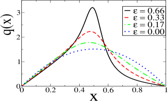
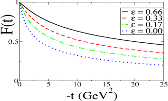
Figure 3: On the left, the quark distribution Eq. (23) is plotted as a function of $x$ for a few values of $\operatorname{\epsilon}$ in GeV². On the right, the form factor calculated from Eqs. (15) and (21) is plotted as a function of $-t$ for a few values of $\operatorname{\epsilon}$ in GeV². The model parameters are arbitrarily chosen as: $M=0.14$ GeV and $m=0.33$ GeV.

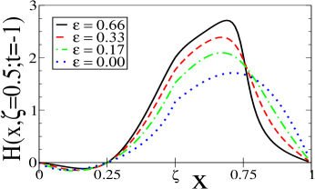
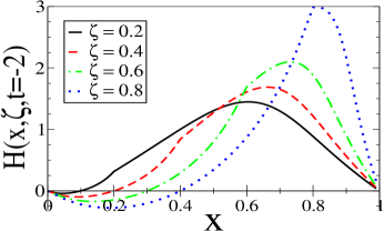
Figure 4: Plots of the GPD calculated from Eqs. (21),(22) and (14). On the left, the GPD is plotted as a function of $x$ for a few values of $\operatorname{\epsilon}$ (in Gev²) at fixed $\zeta=0.5$ and $t=-1.0$ GeV². On the right, the GPD appears at fixed $\operatorname{\epsilon}=0.17$ GeV² and $t=-2.0$ GeV² and is plotted as a function of $x$ for a few values of $\zeta$. The model parameters are arbitrarily chosen as: $M=0.14$ GeV and $m=0.33$ GeV.

IV Cutting rules

In this section, we show there is some hope in working with the model propagator Eq. (1) in Minkowski space. We demonstrate that the quark distribution can be derived by a straightforward generalization of the cutting rules.

Consider the forward Compton amplitude $\mathcal{M}^{\mu\nu}$ depicted in Figure 5. In the Bjorken limit, the imaginary part of this diagram is related to the quark distribution. For simplicity, we can choose a frame in which $\mathbf{q}^{\perp}=0$. The minus-plus component of the forward Compton amplitude in such frames reads

$$i\mathcal{M}^{-+}=-\frac{16N}{\pi^{3}}\int d^{4}k\;(2k^{-}+q^{-})S(k)\;S(k-P)\;S(k)\;(2k^{+}+q^{+})S(k+q).$$ (24)

Figure 5: Handbag diagram for the forward Compton amplitude. Dashed line denotes the cut which yields the quark distribution in the Bjorken limit.

In the scalar particle case, the minus-plus component of the forward Compton amplitude can be used to define the quark distribution in a way analogous to the spin-$\frac{1}{2}$ case. The relation is simply $\Im(\mathcal{M}^{-+})\propto q(x)$, see Tiburzi:2001je . In Eq. (24), we have adjusted the overall normalization so that equality between $\Im(\mathcal{M}^{-+})$ and $q(x)$ holds. With standard perturbative propagators, we could calculate the imaginary part of $\mathcal{M}^{\mu\nu}$ by using the cutting rules, whereby one replaces the cut propagators in Figure 5 by an on-shell prescription, namely

$$S(k)_{\operatorname{\epsilon}=0}\longrightarrow-2\pi i\;\delta(k^{2}-m^{2}).$$ (25)

In Eq. (25), we have specified $\operatorname{\epsilon}=0$ for the case of the free particle propagator. Since large momentum flows through the handle of the handbag, we may neglect the mass of the struck quark and use the standard cutting rule for $S(k+q)$. In the Bjorken limit, we define $x=-q^{2}/2P\cdot q$ which remains finite as $q^{2},P\cdot q\to\infty$ and is kinematically bounded between zero and one. Further we orient our frame of reference so that $q$ has a large minus component in this limit, and consequently $q^{+}=q^{2}/2q^{-}$ is finite. Hence we have the familiar replacement

$$S(k+q)\longrightarrow-\frac{\pi i}{2q^{-}}\;\delta(k^{+}-xP^{+}).$$ (26)

To complete the cut, we must deal with the spectator particle’s complex mass shells. We must worry about the propagator Eq. (1) only where the denominator is zero. Thus we are lead to the cutting rule for the propagator Eq. (1)

$$S(k)\longrightarrow-\pi i\Big{[}\delta(k^{2}-m^{2}+i\operatorname{\epsilon})+\delta(k^{2}-m^{2}-i\operatorname{\epsilon})\Big{]},$$ (27)

which puts the intermediate state on its complex mass shells. Furthermore, the limit $\operatorname{\epsilon}\to 0$ produces the regular cutting rule Eq. (25).

Using this cutting rule for the spectator particle along with Eq. (26), we can deduce the quark distribution from $\Im(\mathcal{M}^{-+})$ in the Bjorken limit

$$q(x)=\frac{4N}{\pi}\int d^{4}k\;\delta(k^{+}-xP^{+})\Big{[}\delta(k^{-}-k_{b}^{-})+\delta(k^{-}-k^{-}_{b^{*}})\Big{]}\frac{xS(k)^{2}}{1-x},$$ (28)

where the light-cone energy poles are given in Eq. (5). Notice the resulting distribution is real and has proper support due to the kinematic constraint $x\in[0,1]$ imposed by the Bjorken limit. Evaluation of the two trivial integrals leaves only the transverse momentum integration

$$q(x)=\frac{N}{\pi}\sum_{\operatorname{\epsilon},\operatorname{\epsilon^{\prime}},\operatorname{\epsilon^{\prime\prime}}=\pm}\int\frac{d\operatorname{\mathbf{k}^{\perp}}}{x(1-x)}\operatorname{D_{\text{W}}}(x,\operatorname{\mathbf{k}^{\perp}},\operatorname{\epsilon},\operatorname{\epsilon^{\prime\prime}}|M^{2})\operatorname{D_{\text{W}}}(x,\operatorname{\mathbf{k}^{\perp}},\operatorname{\epsilon^{\prime}},\operatorname{\epsilon^{\prime\prime}}|M^{2})$$ (29)

where we have defined the Weinberg propagator generalized for complex masses as

$$\operatorname{D_{\text{W}}}(x,\operatorname{\mathbf{k}^{\perp}},\operatorname{\epsilon},\operatorname{\epsilon^{\prime}}|M^{2})^{-1}=M^{2}-\frac{\operatorname{\mathbf{k}^{\perp}}^{2}+m^{2}}{x(1-x)}+\frac{i\operatorname{\epsilon}}{x}+\frac{i\operatorname{\epsilon^{\prime}}}{1-x}.$$ (30)

Evaluation of the $\operatorname{\mathbf{k}^{\perp}}$ integral yields an analytic expression for $q(x)$, which is identical to that obtained from the DD Eq. (23). Notice Eq. (28) is equivalent to evaluating Eq. (4) at $\operatorname{\text{Res}}(k^{-}_{b})+\operatorname{\text{Res}}(k^{-}_{b^{*}})$ and hence the quark distribution is derived as if the complex conjugate spectator poles both lie in the upper-half complex plane! We will understand this better once we analytically continue from Euclidean space.

V Analytic continuation

Above we have seen that modified cutting rules can be used to derive the correct quark distribution function in Minkowski space. In essence the result stems from putting the spectator particle on its complex mass shells. This will be justified by careful analytic continuation of Euclidean space amplitudes. Below we consider the Minkowski space calculation of the generalized parton distribution which cannot be derived by cuts. This will force us to deal with the underlying Wick rotation necessary to define the model in Minkowski space.

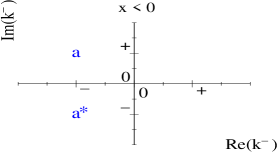
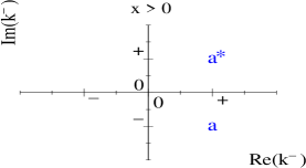
Figure 6: Complex light-cone energy plane for the propagator.

In section III, the model double distributions were calculated in Euclidean space. Thus to calculate related amplitudes in Minkowski space, we must Wick rotate in the complex energy plane: $k^{4}\to ik^{0}$. The analytic continuation can be viewed alternately in the complex light-cone energy plane. For $k^{3}=0$, the rotation is from the $\Im(k^{-})$ axis to the $\Re(k^{-})$ axis. In the general case, such a correspondence can only be made precise by considering the Wick rotation in terms of $k^{0}$ and then boosting to the infinite momentum frame. This requires tedious algebraic manipulations and a proliferation of energy poles and time-ordered diagrams. Indeed it is easier just to imagine the rotation simply and deal with the light-cone singularities. This is the approach we present.

Before tackling generalized parton distributions in Minkowski space, let us imagine a simpler fictitious example. Consider some well-defined Euclidean space amplitude having only poles at $k^{-}_{a}$ and $k^{-}_{a^{*}}$, see Eq. (3). To calculate the amplitude in Minkowski space, we naively integrate along the $\Re(k^{-})$ axis. In general the correct path on which to integrate is one which nears the $\Re(k^{-})$ axis except for detours around energy poles in the first and third quadrants. Such a path is correct since it can be continuously deformed into the Euclidean path. The difference between the naive integration and the correct path is a sum of residues of the Wick poles. The energy poles of our fictitious amplitude are depicted in Figure 6. Their location depends upon the sign of $x=k^{+}/P^{+}$. Thus for this amplitude the correct continuation from Euclidean space is

$$\int d\Im(k^{-})\longrightarrow\int d\Re(k^{-})+2\pi i\big{[}\theta(-x)-\theta(x)\big{]}\operatorname{\text{Res}}(k^{-}_{a^{*}}).$$ (31)

Notice only $k^{-}_{a^{*}}$ is a Wick pole; this is expected because we know the limit $\operatorname{\epsilon}\to 0$ can be analytically continued in the naive fashion. Closing the contour in the upper-half plane to perform the Minkowski space energy integral and evaluate our fictitious amplitude, we pick up $2\pi i[\theta(-x)\operatorname{\text{Res}}(k^{-}_{a})+\theta(x)\operatorname{\text{Res}}(k^{-}_{a^{*}})]$. The net result according to Eq. (31) is thus

$$2\pi i\theta(-x)\big{[}\operatorname{\text{Res}}(k_{a}^{-})+\operatorname{\text{Res}}(k^{-}_{a^{*}})\big{]}.$$

Looking back at Figure 6, the net result after Wick rotation amounts to both poles lying in the same half-plane; or equivalently, we have effectively integrated in either the right- or left-half plane.

The space-like amplitude for the generalized parton distribution can now be continued to Minkowski space and hence be evaluated by projecting onto the light cone. To do so, we refer to Figure 2 and insert the non-local light-cone operator $\phi(0)i\overset{\leftrightarrow}{D}{}^{+}\phi(z^{-})$ in place of the local twist-two operators denoted by a cross in the Figure. Here the plus-component picks out the leading-twist contribution according to light-cone power counting. Thus in momentum space, we arrive at

$$H(x,\zeta,t)=\frac{2N/\pi^{2}}{1-\zeta/2}\int d^{4}k\;\delta(k^{+}-xP^{+})\;(2k^{+}+\Delta^{+})\;S(k)S(k-P)S(k+\Delta).$$ (32)

Above we have included the $\zeta$-dependent pre-factor to normalize the action of $\overset{\leftrightarrow}{D}{}^{+}$ between non-diagonal states. The overall normalization is then the same as in Eq. (18). By writing Eq. (32) in Minkowski space, we must also keep in mind the Wick residues implicitly necessary so that Eq. (32) is meaningful. In addition to the poles $k^{-}_{a}$, $k^{-}_{b}$ (given in Eqs. (3) and (5), respectively) and their complex conjugates, the integrand of Eq. (32) also has the poles

$$k_{c}^{-}=-\Delta^{-}+\frac{(\operatorname{\mathbf{k}^{\perp}}+\operatorname{\mathbf{\Delta}^{\perp}})^{2}+m^{2}}{2(k^{+}+\Delta^{+})}-\frac{i\operatorname{\epsilon}}{2(k^{+}+\Delta^{+})}$$ (33)

and $k^{-}_{c^{*}}=(k^{-}_{c})^{*}$. Carrying out the light-cone energy integration in Eq. (32) as well as adding relevant residues resulting from the Wick rotation produces (the subtle details of this calculation appear in the appendix)

$$H(x,\zeta,t)=-2\pi i\;\theta(x)\theta(\zeta-x)\Big{[}\operatorname{\text{Res}}(k^{-}_{a})+\operatorname{\text{Res}}(k^{-}_{a^{*}})\Big{]}+2\pi i\;\theta(x-\zeta)\theta(1-x)\Big{[}\operatorname{\text{Res}}(k^{-}_{b})+\operatorname{\text{Res}}(k^{-}_{b^{*}})\Big{]},$$ (34)

where the residue is of the integrand in Eq. (32). As a result of the effective relocation of poles to the same half-plane as their complex conjugates, the resulting GPD Eq. (34) is real and vanishes outside $x$ from zero to one.

Using the Weinberg propagator Eq. (30), the residues can be compactly written in terms of relative momenta. Defining the relative momentum of the final state as

$$\operatorname{x^{\prime}}=\frac{x-\zeta}{1-\zeta},\quad\quad\operatorname{\mathbf{k}^{\prime\perp}}=\operatorname{\mathbf{k}^{\perp}}+(1-\operatorname{x^{\prime}})\operatorname{\mathbf{\Delta}^{\perp}},$$ (35)

and the relative momentum of the photon as

$$\operatorname{x^{\prime\prime}}=\frac{x}{\zeta},\quad\quad\operatorname{\mathbf{k}^{\prime\prime\perp}}=\operatorname{\mathbf{k}^{\perp}}+\operatorname{x^{\prime\prime}}\operatorname{\mathbf{\Delta}^{\perp}},$$ (36)

the light-cone GPD can be expressed in the form

$$(1-\zeta/2)\;H(x,\zeta,t)=\theta(x)\theta(\zeta-x)\;H_{1}(x,\zeta,t)+\theta(x-\zeta)\theta(1-x)\;H_{2}(x,\zeta,t),$$ (37)

where we have made the abbreviations

$$H_{1}(x,\zeta,t) =(2\operatorname{x^{\prime\prime}}-1)\frac{N}{2\pi}\sum_{\operatorname{\epsilon},\operatorname{\epsilon^{\prime}},\operatorname{\epsilon^{\prime\prime}}=\pm}\int\frac{d\operatorname{\mathbf{k}^{\perp}}}{\operatorname{x^{\prime\prime}}(1-\operatorname{x^{\prime\prime}})(1-x)}\operatorname{D_{\text{W}}}(x,\operatorname{\mathbf{k}^{\perp}},\operatorname{\epsilon},\operatorname{\epsilon^{\prime\prime}}|M^{2})\operatorname{D_{\text{W}}}(\operatorname{x^{\prime\prime}},\operatorname{\mathbf{k}^{\prime\prime\perp}},\operatorname{\epsilon},\operatorname{\epsilon^{\prime}}|\;t\;)$$ (38)

$$H_{2}(x,\zeta,t) =(2x-\zeta)\frac{N}{2\pi}\sum_{\operatorname{\epsilon},\operatorname{\epsilon^{\prime}},\operatorname{\epsilon^{\prime\prime}}=\pm}\int\frac{d\operatorname{\mathbf{k}^{\perp}}}{x(1-x)\operatorname{x^{\prime}}}\operatorname{D_{\text{W}}}(x,\operatorname{\mathbf{k}^{\perp}},\operatorname{\epsilon},\operatorname{\epsilon^{\prime\prime}}|M^{2})\operatorname{D_{\text{W}}}(\operatorname{x^{\prime}},\operatorname{\mathbf{k}^{\prime\perp}},\operatorname{\epsilon^{\prime}},\operatorname{\epsilon^{\prime\prime}}|M^{2}).$$ (39)

Firstly one can see analytically that the correct quark distribution results at zero momentum transfer, namely $H_{2}(x,0,0)=q(x)$, where $q(x)$ is given by Eq. (29). As remarked in section IV, this function is identical to that obtained from the double distribution Eq. (23). Secondly, the resulting light-cone GPD Eq. (37) agrees numerically with that found from the double distribution, via Eq. (14), which is plotted in Figure $4$. Finally the electromagnetic form factor found from the sum rule

$$F(t)=\int_{0}^{1}dx\;H(x,\zeta,t)$$ (40)

agrees numerically with the result of Eq. (15) (which is plotted in Figure $3$). The $\zeta$-independence of Eq. (40) stems from Lorentz invariance which is present, however, not manifest in Eq. (37). Thus with the calculation of Eq. (37) from analytically continuing to Minkowski space, space-like amplitudes now agree with those calculated from the Euclidean space double distribution.

VI Summary

Above we consider calculation of amplitudes for space-like processes using a scalar propagator with one pair of complex conjugate poles. Although we use a scalar model, generalization to higher spins is clear since the energy denominators are universal. Moreover the analysis can be extended easily to the case where vertex functions have complex conjugate singularities. Such models cannot be directly employed in Minkowski space, they must be analytically continued from Euclidean space.

In section II, the problems of using a propagator with complex conjugate poles in Minkowski space are discussed at the level of the quark distribution function. If the model is defined in Minkowski space, one will generally violate the support and positivity properties of the quark distribution. Next in section III, we show the model is perfectly well defined in Euclidean space by calculating non-diagonal matrix elements of twist-two operators. This leads us to the model’s double distribution which we used to calculate parton and generalized parton distributions as well as the electromagnetic form factor.

In the remainder of the paper, we investigate how to calculate amplitudes properly in Minkowski space. Firstly amplitudes dependent on the imaginary part of some set of diagrams can be calculated by using a straightforward generalization of the cutting rules. We apply this to calculate the quark distribution function from the handbag diagram in the Bjorken limit in section IV. Lastly we consider the analytic continuation of space-like amplitudes from Euclidean space. This is complicated by the presence of Wick poles and requires their residues to be appropriately added when amplitudes are calculated. The details of the GPD calculation appear in the Appendix. Resulting functions calculated in Minkowski space after the Wick rotation agree with those obtained from the model defined in Euclidean space.

This work lays the foundation for calculating light-cone dominated amplitudes using meromorphic model propagators and vertices constrained by lattice data and Ward-Takahashi identities. Distribution functions for such models could be calculated rigorously since the pole structure of the propagator is known and relevant integrals converge in the complex light-cone energy plane. As far as light-cone phenomenology is concerned, resulting expressions would be truly Poincaré covariant (as opposed to diagonal with respect to the non-interacting operators) and would satisfy field-theoretic identities. Filling these two gaps is essential for adequate hadronic phenomenology for processes at large momentum transfer. Moreover, such models would help light-cone methods and Dyson-Schwinger studies reach complementary standing.

*

Appendix A Calculation of the GPD

Below we derive Eq. (34) for the GPD in Minkowski space. The details have been relegated here since there is some subtlety. In order to evaluate Eq. (32), which implicitly needs analytic continuation, we must shift the energy integration variable and define a prescription for dealing with vanishing real parts. Let us see how these difficulties arise.

In considering the Wick rotation, one is usually only concerned with the single denominator that results from combining propagators via Feynman parameters. For the moment, let us ignore the complication of complex conjugate pairs of poles. In this case, combining the denominators of Eq. (18) using Feynman parameters results in $[l^{2}-D_{o}(x,y;t)+i\operatorname{\epsilon}]^{-3}$, where $D_{o}$ is given by Eq. (19). Since the bound state is stable and $t$ is space-like, $D_{o}(x,y;t)$ is always positive and hence there are no Wick poles. Moreover, we have shifted the variable $k^{\mu}$ to arrive at $l^{\mu}$.

In analytically continuing the expression with uncombined propagators (and again no complex conjugate poles), we are confronted with a problem. The pole $k_{b}^{-}$, for example, is shifted by the energy $P^{-}$. Thus the location of the singularity in the complex plane will be shifted parallel to the real axis depending upon the relative magnitude of the spectator’s kinetic energy and $P^{-}$. In the schematic example shown in Section V, the pole $k_{a}^{-}$ does not have such a shift. Thus for the $b$ and $c$ poles, the location of the singularities depicted in Figure 6 will shift along the real axis (depending on $P^{-}$ and $\Delta^{-}$) and there will be threshold Wick poles [the threshold is defined when $\Re(k^{-}_{b,c}=0$]. This is unphysical: we just demonstrated the Wick rotation can be done for the combined denominators without crossing any poles. To perform the same Wick rotation at the level of separate propagators, we must use the freedom to shift the energy variable as well as the stability of the bound state.

   

   

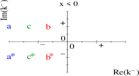
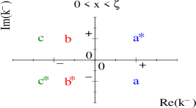
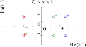
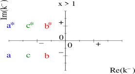
Figure 7: Complex light-cone energy plane for the shifted poles Eq. (43) for the generalized parton distribution.

On the light-cone, the bound state stability condition can be expressed as

$$P^{-}<\frac{\operatorname{\mathbf{k}^{\perp}}^{2}_{\text{rel}}+m^{2}}{2P^{+}x(1-x)},$$ (41)

where $\operatorname{\mathbf{k}^{\perp}}_{\text{rel}}=\operatorname{\mathbf{k}^{\perp}}-x\mathbf{P}^{\perp}$ is the relative transverse momentum of the two constituents. Because we consider the elastic electromagnetic form factor, there is an analogous relation for the final state $P^{\prime}$. Since each propagator contains the kinetic energy of a single particle, the bound state stability condition can never be utilized without shifting $k^{-}$. Yet in order to perform such a shift, the real part of one pole must be zero and hence we must invent a prescription for moving this pole off the Euclidean contour.

We choose the translation: $k^{-}\to k^{-}+\delta k^{-}+\eta$, where $\eta$ is a positive infinitesimal and

$$\delta k^{-}=P^{-}+\frac{\operatorname{\mathbf{k}^{\perp}}^{2}+m^{2}}{2P^{+}(x-1)}.$$ (42)

The resulting poles of the integrand in Eq. (32) we denote

$$\begin{cases}\tilde{k}^{-}_{a}=k^{-}_{a}-\delta k^{-}=-P^{-}+\frac{\operatorname{\mathbf{k}^{\perp}}^{2}+m^{2}}{2P^{+}x(1-x)}-\frac{i\operatorname{\epsilon}}{2P^{+}x}\\ \tilde{k}^{-}_{b}=k^{-}_{b}-\delta k^{-}-\eta=-\eta-\frac{i\operatorname{\epsilon}}{2P^{+}(x-1)}\\ \tilde{k}^{-}_{c}=k^{-}_{c}-\delta k^{-}=-P^{\prime-}+\frac{\operatorname{\mathbf{k}^{\prime\perp}}^{2}+m^{2}}{2P^{\prime+}\operatorname{x^{\prime}}(1-\operatorname{x^{\prime}})}-\frac{i\operatorname{\epsilon}}{2P^{+}(x-\zeta)}\end{cases},$$ (43)

and similarly for their complex conjugate partners. Notice imaginary parts of the poles are unaffected by the energy translation. The $\eta$ prescription has displaced the resulting spectator pole away from the Euclidean path independent of $x$. Moreover the $a$ and $c$ poles have non-zero real parts; so $\eta$ has been set to zero for these poles above.

Using the expressions for the new poles Eq. (43) and the bound state stability condition Eq. (41), we can determine the quadrant location of the singularities independent of $P^{-}$ and $\Delta^{-}$ (see footnote $4$). These quadrant locations are depicted for the full range of $x$ in Figure 7. Accordingly poles in the first and third quadrants are Wick poles. As we saw in Section V, the net result of the analytic continuation is to evaluate the integral by effectively closing the contour in the right- or left-half plane. Hence the GPD Eq. (32) is

$$H(x,\zeta,t)=-2\pi i\;\theta(x)\theta(\zeta-x)\Big{[}\operatorname{\text{Res}}(\tilde{k}^{-}_{a})+\operatorname{\text{Res}}(\tilde{k}^{-}_{a^{*}})\Big{]}+2\pi i\;\theta(x-\zeta)\theta(1-x)\Big{[}\operatorname{\text{Res}}(\tilde{k}^{-}_{b})+\operatorname{\text{Res}}(\tilde{k}^{-}_{b^{*}})\Big{]}.$$ (44)

Evaluating the residues in Eq. (44) yields the result of Section V, namely Eq. (37) which is algebraically equivalent to Eq. (34).

Notice from Figure 7, other $\eta$ prescriptions for the shift, such as $+\frac{\eta}{2P^{+}(x-1)}$, lead to an incorrect result for the case when there are no complex conjugate pairs. The figure shows that the infinitesimal prescription must be positive and independent of the sign of $x$, $x-\zeta$, etc, in order to reproduce the familiar result. It is interesting to note that for $x>1$ in the case without conjugate pairs, all poles of the integrand are Wick poles. Though since the integral is convergent, the sum of these Wick residues vanishes.

The interested reader can verify that the alternate shifts which use the same pole prescription

$$\begin{cases}k^{-}\to k^{-}+\frac{\operatorname{\mathbf{k}^{\perp}}^{2}+m^{2}}{2P^{+}x}+\eta\\ k^{-}\to k^{-}-\Delta^{-}+\frac{(\operatorname{\mathbf{k}^{\perp}}+\operatorname{\mathbf{\Delta}^{\perp}})^{2}+m^{2}}{2P^{+}(x-\zeta)}+\eta\end{cases}$$ (45)

also yield the correct results provided $t$ is space-like.

References

- (1) G. P. Lepage and S. J. Brodsky, Phys. Rev. D 22, 2157 (1980).
- (2) D. Müller, D. Robaschik, B. Geyer, F. M. Dittes and J. Hořejši, Fortsch. Phys. 42, 101 (1994); X.-D. Ji, Phys. Rev. Lett. 78, 610 (1997); Phys. Rev. D 55, 7114 (1997); A. V. Radyushkin, Phys. Lett. B 380, 417 (1996); 385, 333 (1996).
- (3) X.-D. Ji, J. Phys. G 24, 1181 (1998); A. V. Radyushkin, hep-ph/0101225; K. Goeke, M. V. Polyakov and M. Vanderhaeghen, Prog. Part. Nucl. Phys. 47, 401 (2001); A. V. Belitsky, D. Müller and A. Kirchner, Nucl. Phys. B 629, 323 (2002).
- (4) S. J. Brodsky, H. C. Pauli and S. S. Pinsky, Phys. Rept. 301, 299 (1998).
- (5) S. Dalley and B. van de Sande, Phys. Rev. D 59, 065008 (1999); hep-ph/0212086; M. Burkardt and S. K. Seal, Phys. Rev. D 65, 034501 (2002).
- (6) X.-D. Ji, J.-P. Ma and F. Yuan, Nucl. Phys. B 652, 383 (2003); hep-ph/0301141; hep-ph/0304107.
- (7) P. Maris and C. D. Roberts, nucl-th/0301049.
- (8) D. Atkinson and D. W. Blatt, Nucl. Phys. B 151, 342 (1979); C. J. Burden, C. D. Roberts and A. G. Williams, Phys. Lett. B 285, 347 (1992); G. Krein, C. D. Roberts and A. G. Williams, Int. J. Mod. Phys. A 7, 5607 (1992); U. Habel, R. Konning, H. G. Reusch, M. Stingl and S. Wigard, Z. Phys. A 336, 423 (1990); M. Stingl, Z. Phys. A 353, 423 (1996); P. Maris, Phys. Rev. D 52, 6087 (1995); V. N. Gribov, Eur. Phys. J. C 10, 91 (1999).
- (9) M. S. Bhagwat, M. A. Pichowsky and P. C. Tandy, Phys. Rev. D 67, 054019 (2003).
- (10) M. S. Bhagwat, M. A. Pichowsky, C. D. Roberts and P. C. Tandy, nucl-th/0304003.
- (11) R. Alkofer, W. Detmold, C. Fisher and P. Maris, in preparation.
- (12) K. Kusaka, G. Piller, A. W. Thomas and A. G. Williams, Phys. Rev. D 55, 5299 (1997).
- (13) M. B. Hecht, C. D. Roberts and S. M. Schmidt, Phys. Rev. C 63, 025213 (2001).
- (14) A. V. Radyushkin, Phys. Rev. D 56, 5524 (1997); 59, 014030 (1999).
- (15) A. Mukherjee, I. V. Musatov, H. C. Pauli and A. V. Radyushkin, Phys. Rev. D 67, 073014 (2003).
- (16) B. C. Tiburzi and G. A. Miller, Phys. Rev. D 67, 013010 (2003).
- (17) K. J. Golec-Biernat and A. D. Martin, Phys. Rev. D 59, 014029 (1999).
- (18) O. V. Teryaev, Phys. Lett. B 510, 125 (2001).
- (19) M. V. Polyakov and C. Weiss, Phys. Rev. D 60, 114017 (1999).
- (20) A. V. Belitsky, D. Müller, A. Kirchner and A. Schäfer, Phys. Rev. D 64, 116002 (2001).
- (21) B. C. Tiburzi and G. A. Miller, hep-ph/0212238.
- (22) L. Mankiewicz, G. Piller and T. Weigl, Eur. Phys. J. C 5, 119 (1998).
- (23) B. C. Tiburzi and G. A. Miller, Phys. Rev. D 65, 074009 (2002).
- (24) T.-M. Yan, Phys. Rev. D 7, 1780 (1973).