IPPP-03-25
PCPT-03-50
hep-ph/0305163
AUTOMATED RESUMMATION OF FINAL STATE OBSERVABLES IN QCD
We present an innovative method to resum infrared and collinear logarithms appearing in distributions of jet observables in QCD. The method, based on a general master formula with applicability conditions, allows resummations at next-to-leading logarithmic accuracy in an automated way. As a sample application we present resummed results in hadronic dijet events.
1 Jet observables in QCD
A special aspect of QCD in the Standard Model is that the regime where the theory is strongly coupled is within reach of current experiments, and indeed unavoidable. This gives rise to a number of non trivial phenomena, for instance one encounters non-convergent perturbative (PT) expansions and large non-perturbative (NP) corrections even at scales which are, at least formally, within the domain of perturbation theory. One of the main aims of today’s QCD studies is the comprehension of all these phenomena. Apart from its fundamental interest, a detailed QCD description is vital for any precision/search physics in modern colliders.
The study of jet observables, event-shapes and jet-rates, is particularly informative in that these quantities are calculable in perturbation theory with a remarkably high accuracy, but they are still sensitive to NP, low energy physics. For brevity, in the following I will refer to event-shapes only; these are infrared and collinear safe observables describing the topology of the final state in high energy collisions.
In recent years their mean values and distributions have been used to measure the coupling constant , the colour factors and to study their hadronisation corrections. The most discriminatory studies make use of distributions. Integrated distributions are defined by requiring that the value of the observable – a function of all momenta – be less than a fixed value
| (1) |
These distributions are characterised by two kinematical scales, the hard scale of the process (for instance the c.o.m. energy in collisions, the virtuality of the gauge boson in DIS processes, etc.) and an observable scale whose magnitude is determined by the typical momenta of secondary emissions. In the more exclusive kinematical region there is a strong ordering between these two scales, so that the distribution Eq. 1 contains (large) logarithms of the ratio of the two scales . They compensate the smallness of , and to make predictions one needs to resum logarithmically enhanced (next-to-leading NLL) terms to all orders, while in the region where fixed order (next-to-leading NLO) predictions are reliable.
It is interesting to compare today’s effort required to obtain NLO and NLL predictions. To compute distributions at a given PT order one needs to know the emission probabilities (the squared matrix elements) at that perturbative order. Given the QCD Lagrangian, these quantities are calculable in principle at any order, though technically it becomes extremely difficult to go beyond NLO. Since PT matrix elements are independent of the observable, they can be implemented in a general way in Fixed Order Monte Carlos. These are then widely exploited for experimental studies, the only additional input needed being the definition of the specific observable in the form of a computer routine. Obtaining NLL descriptions also requires the knowledge of the emission probabilities. These quantities mix different logarithmic orders, so that one needs to reorganise the PT series so as to account for (resum) all leading (LL) and next-to-leading logarithmic (NLL) terms. Also, since one is resumming terms to all PT orders, one needs to know the value of the observable given an arbitrary number of secondary emissions. These are the reasons why, so far, the description of each observable has required a separate analytical calculation, this limits the experimental study of resummed predictions, as compared to fixed order ones.
2 Automated resummation
The aim of this project is to automate the NLL resummation of jet observables, so as to ease their experimental analysis. To achieve this goal one has to understand the origin of all NLL enhanced terms in observable distributions. This reduces to two steps: one needs to know the behaviour of the observable when only one soft-collinear (SC) gluon is present in the final state (single emission properties); furthermore one needs to understand the way in which all emissions coherently determine the value of the observable (multiple emission properties).
2.1 Single emission properties
To describe the behaviour of the observable due to a single emission we fix an (arbitrary) Born event and simulate the emission of one soft gluon collinear to each hard parton (leg) . We assume that the observable can be parameterised as
| (2) |
where , denote respectively the transverse momentum and the rapidity with respect to the emitting hard leg and is the azimuthal angle with respect to a plane. Our numerical code verifies automatically the assumed parameterisation and determines the coefficients and the functions . This knowledge allows us to compute all the NLL terms which account for hard collinear emissions, soft large angle radiation and inclusive gluon splittings (running of the coupling). This gives rise to a single (or simple) distribution , where is a LL Sudakov exponent (complete formulae can be found elsewhere). It also happens, by construction, that is the full NLL resummed distribution for a simpler observable whose value is determined only by the largest emission
| (3) |
2.2 Multiple emission properties
To fully resum the observable at NLL one also needs to relate the value of the observable to the momenta of all secondary emissions, i.e. to understand the observable specific mismatch between the full observable and its simplified variant . An analytical treatment of this requires a detailed insight in the kinematics of the recoiling hard partons and, for jet-rates, of the recombination procedure, but this effect can be computed numerically in a general way and is given as a pure NLL function , with .
2.3 The master formula and its applicability conditions
The knowledge of the single and multiple emission properties is combined in a master formula
| (4) |
The formula Eq. 4 does of course not apply to all final state observables in QCD and is accompanied by a list of conditions the observable has to fulfil: it should be recursively infrared and collinear safe; should vanish in the Born limit; should be continuously global; should behave as assumed in Eq. 2 when only one SC emission is present; additionally it should, at the present stage, satisfy some minor (technical) requirements. While this might seem a long list practically the limiting condition is the requirement of globalness, while all other conditions are satisfied by all observables resummed so far. Most importantly an essential feature of our code is the ability to verify all properties automatically and to resum the observable only when the correctness of the result is guaranteed at NLL accuracy.
2.4 Sample output: first ever resummations in hadronic dijet production
| leg | |||||
|---|---|---|---|---|---|
| 1 | 1 | 0 | tabulated | 2 | -0.2201 |
| 2 | 1 | 0 | tabulated | 2 | -0.2201 |
| 3 | 1 | 0 | 2 | - | |
| 4 | 1 | 0 | 2 | - |
The most interesting application of our method is the resummation of observables in hadronic dijet events. As an example we present here results for the indirectly global thrust minor aaaNote that the second term guarantees the continuous globalness of the observable.
| (5) |
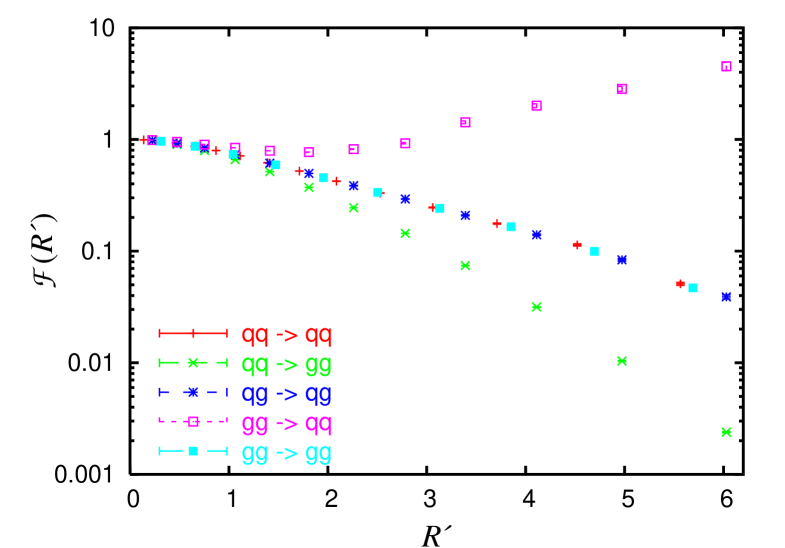
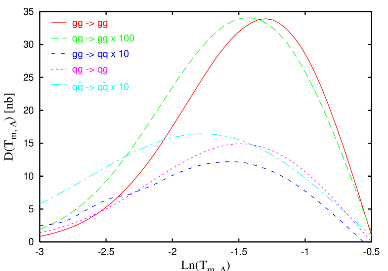
here denote the momenta transverse to the beam, the momenta out of the plane defined by the beam-axis and the transverse thrust axis and denotes a rapidity cut. The program verifies all applicability conditions; tabulates the single emission properties, see Tab. 1; computes for all colour configurations the multiple emission function , see Fig. 1 (left); and exploits the master formula Eq. 4 to obtain the full NLL resummed prediction. Fig.1 (right) shows differential distributions, for several underlying hard subprocesses, for the Tevatron run II regime, GeV. We select events having two outgoing jets with GeV and , fix , use the CTEQ6M parton density set, corresponding to and set the factorisation and renormalisation scales and at the partonic c.o.m. energy.


2.5 Final remarks, conclusions and outlook
Results presented here have the quality of analytic NLL predictions, though no human intervention is needed. This implies that any hadronisation model can be applied, studies of renormalisation and factorisation scale dependence can be carried out and, since the answer is free of spurious subleading terms, a matching with fixed order is feasible.
The first step in this project has been the numerical computation of multiple-emission effects, which allowed us to resum three observables in -collisions at a time. We have now a code which fully automates the resummation of a large class of jet observables; as a result we obtained the first ever resummations in hadronic dijet production. As a next step we aim to automate the matching with fixed order results. This will open up the possibility to carry out a vast amount of phenomenological studies.
Acknowledgements
I am enjoying working at this project with Andrea Banfi and Gavin Salam. A special thank to Yuri Dokshitzer and Pino Marchesini for stimulating conversations and precious suggestions.
References
References
- [1] S. Bethke, J. Phys. G 26, R27 (2000).
- [2] S. Kluth et al., Eur. Phys. J. C 21, 199 (2001) and references therein.
- [3] P. A. Movilla Fernandez, S. Bethke, O. Biebel and S. Kluth, Eur. Phys. J. C 22, 1 (2001).
- [4] D. Graudenz, arXiv:hep-ph/9710244; J. Campbell and R. K. Ellis, Phys. Rev. D 65 (2002) 113007 ; Z. Nagy, Phys. Rev. Lett. 88, 122003 (2002).
- [5] A. Banfi, G. P. Salam and G. Zanderighi, arXiv:hep-ph/0304148 and in preparation.
- [6] A. Banfi, G. P. Salam and G. Zanderighi, JHEP 0201, 018 (2002).
- [7] M. Dasgupta and G. P. Salam, Phys. Lett. B 512, 323 (2001); JHEP 0208, 032 (2002) and references therein.
- [8] J. Pumplin et al. JHEP 0207, 012 (2002).