ELECTROWEAK PRECISION TESTS OF LITTLE HIGGS THEORIES

Little Higgs theories are a fascinating new idea to solve the little hierarchy problem by stabilizing the Higgs mass against one-loop quadratically divergent radiative corrections. In this talk I give a brief overview of the idea, focusing mainly on the littlest Higgs model, and present a sampling of the electroweak precision constraints.

1 Introduction

It is well known that the Higgs boson mass is quadratically sensitive to heavy physics. The quadratic sensitivity arises from Yukawa couplings, gauge couplings, and the Higgs quartic coupling. Naturalness suggests the cutoff scale of the Standard Model (SM) should be only a loop factor higher than the Higgs mass,

$$\Lambda\mathrel{\>{\hbox{\raise 1.50696pt\hbox{$<$}}\kern-3.8889pt\kern-3.8889pt\hbox{\lower 2.79857pt\hbox{$\sim$}}}\>}4\pi m_{h}\;.$$ (1)

However, there are many probes of physics beyond the SM at scales ranging from a few to tens of TeV. In particular, four-fermion operators that give rise to new electroweak contributions generally constrain the new physics scale to be more than a few TeV, and some new flavor-changing four-fermion operators are constrained even further, to be above the tens of TeV level. With mounting evidence $\!{}^{{\bf?}}$ for the existence of a light Higgs with mass $\mathrel{\>{\hbox{\raise 1.50696pt\hbox{$<$}}\kern-3.8889pt\kern-3.8889pt\hbox{\lower 2.79857pt\hbox{$\sim$}}}\>}200$ GeV, see Fig. 1,

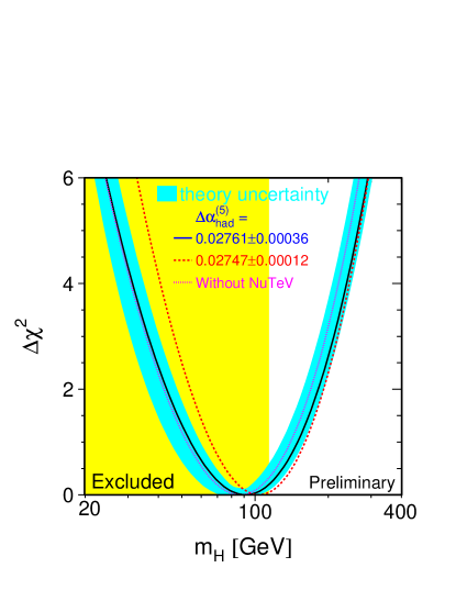
Figure 1: Best fit of the electroweak data as a function of the Higgs mass. Taken from Ref. $\!{}^{{\bf?}}$

we are faced with understanding why the Higgs mass is so light compared with radiative corrections from cutoff-scale physics that appears to have been experimentally forced to be well above the TeV level. The simplest solution to this “little hierarchy problem” is to fine-tune the bare mass against the radiative corrections, but this is widely seen as being unnatural.

There has recently been much interest $\!{}^{{\bf?},{\bf?},{\bf?},{\bf?},{\bf?},{\bf?},{\bf?},{\bf?},{\bf?},{\bf?},{\bf?},{\bf?},{\bf?},{\bf?},{\bf?},{\bf?},{\bf?}}$ in a new approach to solving the little hierarchy problem, called little Higgs models. These models have a larger gauge group structure appearing near the TeV scale to which the electroweak gauge group is embedded. The novel feature of little Higgs models is that there are approximate global symmetries that protect the Higgs mass from acquiring one-loop quadratic sensitivity to the cutoff. This happens because the approximate global symmetries ensure that the Higgs can acquire mass only through “collective breaking”, or multiple interactions. In the limit that any single coupling goes to zero, the Higgs becomes an exact (massless) Goldstone boson. Quadratically divergent contributions are therefore postponed to two-loop order, thereby relaxing the tension between a light Higgs mass and a cutoff of order tens of TeV. Schematically, this can be written as

$$\Lambda\mathrel{\>{\hbox{\raise 1.50696pt\hbox{$<$}}\kern-3.8889pt\kern-3.8889pt\hbox{\lower 2.79857pt\hbox{$\sim$}}}\>}(4\pi)^{2}m_{h}\;.$$ (2)

Since I am giving this talk at Moriond, it seems appropriate to borrow a French colloquialism by saying that this “2” in the exponent is the raison d’être of little Higgs theories.

There are now several published little Higgs models; Table 1 summarizes those that have appeared as of this conference. Little Higgs models can be understood from a variety of perspectives including deconstruction, analogy to the chiral Lagrangian, etc., all of which have appeared in the literature. In the following I have chosen to discuss the operational character of little Higgs models by analogy to custodial $SU(2)$ of the SM. This at least provides my own (odd?) personal perspective, however imperfect the analogy may be.

The Higgs field of the SM transforms as a complex doublet under $SU(2)_{L}$, but more generally as a $\mathbf{4}$ of an $SO(4)$ global symmetry that rotates the four real scalar fields among themselves. An $SU(2)$ subgroup of the $SO(4)$ symmetry is gauged, corresponding to $SU(2)_{L}$. When the Higgs acquires a vacuum expectation value, the $SO(4)$ global symmetry is broken to $SO(3)\sim SU(2)$. This residual, or “custodial” $SU(2)_{c}$ is an approximate global symmetry of the Higgs sector in the SM. If $SU(2)_{c}$ were exact, it would imply an interesting relation among the gauge boson masses, namely $M_{W}/M_{Z}=1$. But, gauging hypercharge is incompatible with custodial $SU(2)$, which is manifested at tree-level by the relation

$$\frac{M_{W}^{2}}{M_{Z}^{2}}=\frac{g^{2}}{g^{2}+g^{\prime 2}}\;.$$ (3)

Nevertheless there is a smooth transition in which the global custodial $SU(2)$ symmetry is restored when $g^{\prime}\rightarrow 0$.

Little Higgs theories have several similarities to custodial $SU(2)$ of the SM. In the following, I will use the littlest Higgs model $\!{}^{{\bf?}}$ as my example. The littlest Higgs model has a global $SU(5)$ symmetry with a single scalar non-linear sigma model field in the $\mathbf{15}$ of $SU(5)$ [just as in the SM there is a global $SO(4)$ symmetry with a single Higgs linearly realized in a $\mathbf{4}$ of $SO(4)$]. The symmetric tensor acquires an expectation value breaking global $SU(5)$ down to global $SO(5)$ [just as the Higgs acquiring an expectation value breaking global $SO(4)$ down to $SU(2)_{c}$.] An $[SU(2)\times U(1)]^{2}$ subgroup of $SU(5)$ is gauged [just as an $SU(2)_{L}$ subgroup of $SO(4)$ was gauged]. The expectation value of the symmetric tensor breaks $[SU(2)\times U(1)]^{2}\rightarrow SU(2)_{L}\times U(1)_{Y}$ [just as the Higgs breaks $SU(2)_{L}\times U(1)_{Y}\rightarrow U(1)_{em}$]. As the gauge couplings for, say, $SU(2)_{1}\times U(1)_{1}$ are turned off, $g_{1},g_{1}^{\prime}\rightarrow 0$, an $SU(3)_{1}$ subgroup of the $SU(5)$ global symmetry is restored [just as turning off hypercharge $g^{\prime}\rightarrow 0$ restores custodial $SU(2)$]. The same procedure can be done for $SU(2)_{2}\times U(1)_{2}$. In either case, the restoration of part of the global symmetry by ungauging some part of the gauge symmetry leads to an “interesting relation”, for little Higgs this is $m_{h}\rightarrow 0$ [just as $M_{W}/M_{Z}\rightarrow 1$]. Of course the symmetry explanation for the masslessness of the Higgs is because it represents (four of eight) Goldstone bosons of spontaneously broken $SU(3)$. Since one arrives at the same result regardless of which set of $SU(2)\times U(1)$ symmetries are ungauged, one concludes that the Higgs cannot acquire a mass from interactions only with one gauge coupling. Hence, the Higgs does not acquire a quadratic divergence from gauge loops to one-loop order because the Higgs is protected by an approximate global symmetry.

For there to be no one-loop quadratic divergence from also interactions with fermions (in particular, top quarks) and with itself through the quartic coupling, the approximate global symmetries must be respected by these interactions. This can be done for the top Yukawa by adding a vector-like pair of fermions $\tilde{t},\tilde{t}^{\prime}$ and arranging that the top quark acquires a mass through collective breaking. The details for each model can be found in the literature. Similarly the quartic coupling must also arise through collective breaking. In practice this means there are new particles near the TeV scale that have the effect of canceling off the quadratic divergences of the Higgs. In the littlest Higgs model, for example, there are four new gauge bosons $W_{H}^{a},B_{H}$, a vector-like pair of quarks that mix to yield the right-handed top quark, and a new scalar field that is a triplet of $SU(2)_{L}$. These states successfully cancel off the quadratic divergences of the Higgs so long as their masses are not too far from the TeV scale.

	Global		# of light	Higgs
Model Name	Symmetry	Gauge Symmetry	Higgs doublets	triplet vev?
Minimal Moose $\!{}^{{\bf?}}$	$SU(3)^{8}$	$SU(3)\times SU(2)\times U(1)$	$2$	yes
Littlest Higgs $\!{}^{{\bf?}}$	$SU(5)$	$[SU(2)\times U(1)]^{2}$	$1$	yes
Antisymmetric condensate $\!{}^{{\bf?}}$	$SU(6)$	$[SU(2)\times U(1)]^{2}$	$2$	no
Simple group $\!{}^{{\bf?}}$	$SU(4)^{4}$	$SU(4)\times U(1)$	$2$	no
Custodial SU(2) Moose $\!{}^{{\bf?}}$	$SO(5)^{8}$	$SO(5)\times SU(2)\times U(1)$	$2$	yes

Table 1: Little Higgs models as of March 2003.

New TeV mass gauge bosons can be problematic if the SM gauge bosons mix with them or if the SM fermions couple to them. This is because modifications of the electroweak sector are usually tightly constrained by precision electroweak data (see Refs. $\!{}^{{\bf?},{\bf?},{\bf?},{\bf?}}$ for example). Consider the modification to the coupling of a $Z$ to two fermions and (separately) the modification to the vacuum polarization of the $W$, as shown in Fig. 2. These are among the best measured electroweak parameters that agree very well with the SM predictions (using $M_{Z}$, $G_{F}$, and $\alpha_{em}$ as inputs): both of these observables have been measured to $\pm 0.2\%$ to 95% C.L. Generically the corrections to these observables due to heavy $U(1)$ gauge bosons and heavy $SU(2)$ gauge bosons can be simply read off from Fig. 2 as

$$\frac{\delta\Gamma_{Z}}{\Gamma_{Z}}\sim 1+c_{1}\frac{v^{2}}{f^{2}}\quad,\quad\frac{\delta M_{W}^{2}}{M_{W}^{2}}\sim 1+c_{2}\frac{v^{2}}{f^{2}}\;,$$ (4)

where $f$ is roughly the mass of the heavy gauge boson, $c_{1}$ and $c_{2}$ parameterize the strength of the couplings between heavy-to-light fields. For $c_{1}\sim 1$ or $c_{2}\sim 1$, it is trivial to calculate the electroweak bound on $f$,

$$f>5.5\;\mbox{TeV}\quad\mbox{to 95\% C.L.}\;.$$ (5)

Notice that even if the coupling of light fermions to the heavy gauge bosons were zero ($c_{1}=0$), maximal mixing among $SU(2)$ gauge bosons ($c_{2}=1$) is sufficient to place a strong constraint on the scale of new physics.

Figure 2: Corrections to $\Gamma_{Z}$ and to $M_{W}^{2}$ through mixing with heavy gauge bosons.

In principle one needs only calculate these coefficients (and those of other electroweak observables) and combine them using a global fit to determine the bounds from electroweak precision data. This is straightforward but technical, and so I refer interested readers to the original papers $\!{}^{{\bf?},{\bf?}}$ for details.

At this point I should stress that mixing between heavy and light gauge bosons, as well as the coupling of heavy gauge bosons to light fermions is a parameter-dependent and/or model-dependent issue that does not directly constrain the little Higgs mechanism for canceling quadratic divergences. Here I shall parameterize simple examples that will show what direction the electroweak constraints tend to “push” on the parameter space of models. Consider the littlest Higgs model with light fermions coupling to only $SU(2)_{1}\times U(1)_{1}$. The four high energy gauge groups have four couplings that match onto the well-known $SU(2)_{L}\times U(1)_{Y}$ couplings, leaving two parameters that we take to be angles defined by $c\equiv\cos\theta=g/g_{2}$ and $c^{\prime}\equiv\cos\theta^{\prime}=g^{\prime}/g^{\prime}_{2}$. To ensure the high energy gauge couplings $g_{1,2},g^{\prime}_{1,2}$ are not strongly coupled, the angles $c,s,c^{\prime},s^{\prime}$ cannot be too small. We conservatively allow for $c,s,c^{\prime},s^{\prime}>0.1$, or equivalently $0.1<c,c^{\prime}<0.995$. We allow the symmetry breaking scale $f$ to take on any value (although for small enough $f$ there will be constraints from direct production of $B_{H}$). The general procedure we to systematically step through values of $c$ and $c^{\prime}$, finding the lowest value of $f$ that leads to a shift in the $\chi^{2}$ corresponding to the 68%, 95%, and 99% confidence level (C.L.). For a three-parameter fit, this corresponds to a $\Delta\chi^{2}$ of about $3.5$, $7.8$, $11.3$ from the minimum, respectively. The bound on $f$ is perhaps best illustrated as a function of $c^{\prime}$, as shown in Fig. 3. The shaded area below the lines shows the region of parameter space excluded by precision electroweak data. Note that we numerically found the value of $c$ that gave the least restrictive bound on $f$ for every $c^{\prime}$. For a specific choice of $c$ the bound on $f$ can be stronger as shown by the different contours in the figure.

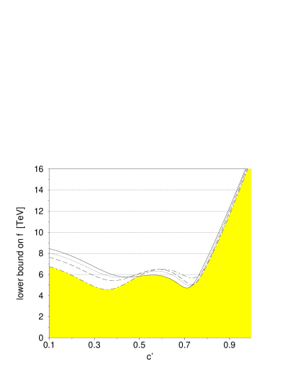
Figure 3: For the littlest Higgs model with light fermions coupling only to $SU(2)_{1}\times U(1)_{1}$, the region of parameters excluded to 95% C.L. is shown as a function of $c^{\prime}$. The region below the contours is excluded to 95% C.L. for $c$ equal to $0.1$ (solid), $0.5$ (dotted), $0.7$ (dashed), $0.99$ (dot-dashed). The shaded region is excluded for any choice of $c$.

Light fermions that are charged under just $U(1)_{1}$ maximally couple to both $B_{L}$ and $B_{H}$. In the littlest Higgs model, $B_{H}$ is curiously light due to group theoretic factors, and is one source of the strong constraints on the model. Although the top quark must have certain well-defined couplings to $U(1)_{1}$ and $U(1)_{2}$ to ensure that the global symmetries are preserved by its Yukawa interaction, the light fermions have no such restriction since their one-loop quadratically divergent contribution to the Higgs mass is numerically negligible. In Ref. $\!{}^{{\bf?}}$ we considered varying the $U(1)$ charges of the light fermions. This results in a free parameter $R$ that characterizes how strongly a given fermion is coupling to $U(1)_{1}$ ($R$ times its hypercharge) and $U(1)_{2}$ ($1-R$ times its hypercharge). If we wish to maintain integer powers of the non-linear sigma model field when writing Yukawa couplings, then $R$ can only take on fractional integer powers $0,1/5,2/5,\ldots$. Three interesting cases are $R=1$, the choice in Fig. 3; $R=4/5$, the choice that leads to dimension-4 Yukawa couplings; and $R=3/5$, the choice that is identical to that of the top quark.

In Fig. 4 a contour plot for fixed $R=3/5,4/5,1$ shows the allowed range of parameter space at 95% C.L. for both $c$ and $c^{\prime}$ showing the size of the allowed region of parameter space for a given value of $R$. Unlike what we found for $R=1$, it is clear that for $R=3/5$ there are restricted regions of parameter space where the bound on $f$ is in the $1$-$2$ TeV.

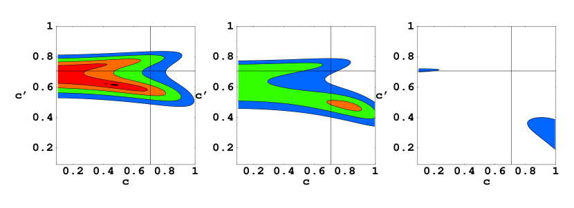
Figure 4: Contours of the minimum allowed values of $f$ at 95% C.L. for $a=1$ and $R=3/5$ (left graph) $R=4/5$ (center graph) $R=1$ (right graph). The black contour is for $f<1$ TeV, red is $f<2$ TeV, orange is $f<3$ TeV, green is $f<4$ TeV, blue is $f<5$ TeV, and white is $f>5$ TeV.

This illustrates that varying the strength of the coupling of light fermions to $B_{H}$ leads to quite dramatically different constraints on the littlest Higgs model.

One alternative that avoids all of the difficulties associated with $B_{H}$ is to simply gauge $U(1)_{Y}$. This leads to a one-loop quadratic divergence proportional to $g^{\prime 2}$, but this is numerically small if the cutoff scale is around 10 TeV. Now it becomes more important to examine a fuller set of contributions to the electroweak observables. There are (at least) two additional effects: in the littlest Higgs model there is an $SU(2)_{L}$ triplet scalar field that acquires a vev $v^{\prime}={\cal O}(v^{2}/f)$, leading to an additional tree-level contribution, while at one-loop there are significant contributions from the heavy top. For this discussion let me consider only the triplet vev in addition to heavy gauge boson exchange. The triplet vev can be calculated by minimizing the effective potential; the details are in Refs. $\!{}^{{\bf?},{\bf?}}$. One finds

$$|v^{\prime}|^{2}=\frac{v^{4}}{16f^{2}}\left[\frac{2\lambda}{a(g_{1}^{2}+g_{1}^{\prime 2})}-1\right]^{2}~{}.$$ (6)

in terms of a single parameter $a\sim{\cal O}(1)$ in the Coleman-Weinberg effective potential and the Higgs quartic coupling $\lambda$. We can then recalculate the electroweak observables including a triplet vev, and for a littlest-type Higgs model in which only $SU(2)_{1}\times SU(2)_{2}\times U(1)_{Y}$ is gauged the result shown in Fig. 5. Interestingly, for suitable $SU(2)_{1,2}$ gauge couplings $g_{2}\gg g_{1}$ and an order one parameter in the Coleman-Weinberg potential, the bound on $f$ is $1$-$2$ TeV.

There are several other variations of the littlest Higgs model, and variations in the global symmetries that lead to other interesting constraints. Here I restricted myself to presenting only a small sampling of the little Higgs models or variations, and their electroweak constraints. There are a few general lessons that are already clear: First, for generic choices of couplings of light fermions to heavy gauge bosons (such as coupling to just $SU(2)_{1}\times U(1)_{1}$), or generic light/heavy gauge boson mixing (such as $c\sim 1/\sqrt{2}$), the bound on the symmetry breaking scale $f$ is maximized to of order $4$-$5$ TeV. In the littlest Higgs model, a lower bound on $f$ can be translated into a lower bound on the mass the vector-like quarks $m\mathrel{\>{\hbox{\raise 1.50696pt\hbox{$>$}}\kern-3.8889pt\kern-3.8889pt\hbox{\lower 2.79857pt\hbox{$\sim$}}}\>}\sqrt{2}f$, and then translated into the minimal amount of fine-tuning to obtain a light Higgs. However, decoupling the light fermions from the heavy $B$ gauge boson (either exactly or approximately as shown above for $R=3/5$) or eliminating the heavy $B$ gauge boson entirely from the spectrum, while choosing the observed $W$ gauge boson to be nearly pure $W_{1}$ generally allows the symmetry breaking scale $f$ to be $1$-$2$ TeV. In some models, bounding $f$ does not directly imply an upper bound on the amount of fine-tuning; other parameters in the theory that can be suitably chosen to, for example, keep the heavy vector-like quarks significantly lighter than their heavier gauge boson cousins. We can surely expect exciting further developments in new little Higgs models and UV completions!

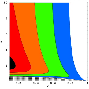
Figure 5: Contour plot of the allowed values of $f$ as a function of the parameters $a$ and $c$. The allowed contours correspond to less than $1,2,3,4,5$ TeV. The grey shaded region at the bottom corresponds to the region excluded by requiring a positive triplet (mass)².

References

References

- [1] LEP Electroweak Working Group, LEPEWWG/2002-01.
- [2] N. Arkani-Hamed, A. G. Cohen and H. Georgi, Phys. Lett. B 513, 232 (2001) [arXiv:hep-ph/0105239].
- [3] N. Arkani-Hamed, A. G. Cohen, E. Katz, A. E. Nelson, T. Gregoire and J. G. Wacker, JHEP 0208, 021 (2002) [arXiv:hep-ph/0206020].
- [4] N. Arkani-Hamed, A. G. Cohen, E. Katz and A. E. Nelson, JHEP 0207, 034 (2002) [arXiv:hep-ph/0206021].
- [5] T. Gregoire and J. G. Wacker, JHEP 0208, 019 (2002) [arXiv:hep-ph/0206023]. arXiv:hep-ph/0207164.
- [6] I. Low, W. Skiba and D. Smith, Phys. Rev. D 66, 072001 (2002) [arXiv:hep-ph/0207243].
- [7] J. G. Wacker, arXiv:hep-ph/0208235.
- [8] M. Schmaltz, Nucl. Phys. Proc. Suppl. 117, 40 (2003) [arXiv:hep-ph/0210415].
- [9] C. Csáki, J. Hubisz, G. D. Kribs, P. Meade and J. Terning, arXiv:hep-ph/0211124.
- [10] J. L. Hewett, F. J. Petriello and T. G. Rizzo, arXiv:hep-ph/0211218.
- [11] G. Burdman, M. Perelstein and A. Pierce, arXiv:hep-ph/0212228.
- [12] T. Han, H. E. Logan, B. McElrath and L. T. Wang, Phys. Rev. D 67, 095004 (2003) [arXiv:hep-ph/0301040].
- [13] D. E. Kaplan and M. Schmaltz, arXiv:hep-ph/0302049.
- [14] C. Dib, R. Rosenfeld and A. Zerwekh, arXiv:hep-ph/0302068.
- [15] T. Han, H. E. Logan, B. McElrath and L. T. Wang, arXiv:hep-ph/0302188.
- [16] S. Chang and J. G. Wacker, arXiv:hep-ph/0303001.
- [17] C. Csáki, J. Hubisz, G. D. Kribs, P. Meade and J. Terning, arXiv:hep-ph/0303236.
- [18] A. E. Nelson, arXiv:hep-ph/0304036.
- [19] R. S. Chivukula, N. Evans and E. H. Simmons, Phys. Rev. D 66, 035008 (2002) [arXiv:hep-ph/0204193].
- [20] R. S. Chivukula, E. H. Simmons and J. Terning, Phys. Lett. B 346, 284 (1995) [arXiv:hep-ph/9412309].
- [21] C. Csáki, J. Erlich and J. Terning, Phys. Rev. D 66, 064021 (2002) [arXiv:hep-ph/0203034].
- [22] C. Csáki, J. Erlich, G. D. Kribs and J. Terning, Phys. Rev. D 66, 075008 (2002) [arXiv:hep-ph/0204109].