On theory of Landau-Pomeranchuk-Migdal effect

Abstract

The cross section of bremsstrahlung from high-energy electron suppressed due to the multiple scattering of an emitting electron in a dense media (the LPM effect) is discussed. Development of the LPM effect theory is outlined. For the target of finite thickness one has to include boundary photon radiation as well as the interference effects. The importance of multiphoton effects is emphasized. Comparison of theory with SLAC data is presented.

1 Introduction

The process of photon radiation takes place not in one point but in some domain of space-time, in which a photon (an emitted wave in the classical language) is originating. The longitudinal dimension of this domain is called the formation (coherence) length $l_{f}$

$$l_{f0}(\omega)=2\varepsilon\varepsilon^{\prime}/\omega m^{2},$$ (1)

where $\varepsilon(\varepsilon^{\prime})$ is the energy of the initial (final) electron, $\omega$ is the photon energy, $\varepsilon^{\prime}=\varepsilon-\omega$, $m$ is the electron mass, we employ units such that $\hbar=c=1$. So for ultrarelativistic particles the formation length extends substantially. For example for $\varepsilon=25$ GeV and emission of $\omega=100$ MeV photon, $l_{f}=10\mu$m, i.e.$\sim 10^{5}$ interatomic distances.

Landau and Pomeranchuk were the first to show that if the formation length of the bremsstrahlung becomes comparable to the distance over which the multiple scattering becomes important, the bremsstrahlung will be suppressed [1]. They considered radiation of soft photons. Migdal [2] developed a quantitative theory of this phenomenon. Now the common name is the Landau- Pomeranchuk -Migdal (LPM) effect.

Let us estimate a disturbance of the emission process due to a multiple scattering. As it is known, the mean angle of the multiple scattering at some length $l_{f}$ is

$$\vartheta_{s}=\sqrt{\vartheta_{s}^{2}}=\varepsilon_{s}/\varepsilon\sqrt{l_{f}/2L_{rad}},\quad\varepsilon_{s}=m\sqrt{4\pi/\alpha}=21.2~{}{\rm MeV},$$ (2)

where $\alpha=e^{2}=1/137$, $L_{rad}$ is the radiation length. Since we are interesting in influence of the multiple scattering on the radiation process we put here the formation length (1). One can expect that when $\vartheta_{s}\geq 1/\gamma$ this influence will be substantial. From this inequality we have

$$\varepsilon^{\prime}/\varepsilon_{LP}\geq\omega/\varepsilon,\quad\varepsilon_{LP}=m^{4}L_{rad}/\varepsilon_{s}^{2},$$ (3)

here $\varepsilon_{LP}$ is the characteristic energy scale, for which the multiple scattering will influence the radiation process for the whole spectrum. It was introduced in [1] and denoted by $E_{0}=\varepsilon_{LP}$. For tungsten we have $\varepsilon_{LP}=2.72$ TeV, and similar values for the all heavy elements. For light elements the energy $\varepsilon_{LP}$ is much larger. When $\varepsilon\ll\varepsilon_{LP}$ the multiple scattering will influence emission of soft photons only with energy $\omega\leq\omega_{LP}=\varepsilon^{2}/\varepsilon_{LP}$, e.g. for particles with energy $\varepsilon=25$ GeV one has $\omega_{LP}\simeq 230$ MeV. Of course, we estimate here the criterion only. For description of the effect one has to calculate the probability of the bremsstrahlung taking into account multiple scattering.

2 The LPM effect in a infinite medium

We consider first the case where the formation length is much shorter than the thickness of a target $l(l_{f0}\ll l)$. The basic formulas for probability of radiation under influence of multiple scattering were derived in [3]. The general expression for the radiation probability obtained in framework of the quasiclassical operator method (Eq.(4.2) in [4])was averaged over all possible particle trajectories. This operation was performed with the aid of the distribution function, averaged over atomic positions in the scattering medium and satisfying the kinetic equation. The spectral distribution of the probability of radiation per unit time was reduced in [5] to the form

$$dW/d\omega=(2\alpha/\gamma^{2}){\rm Re}\int_{0}^{\infty}dte^{-it}\left[R_{1}\varphi_{0}(0,t)+R_{2}{\bf p}\mbox{\boldmath$\varphi$}(0,t)\right],$$ (4)

where $R_{1}=\omega^{2}/\varepsilon\varepsilon^{\prime},\quad R_{2}=\varepsilon/\varepsilon^{\prime}+\varepsilon^{\prime}/\varepsilon$, and the functions $\varphi_{\mu}~{}(\varphi_{0},\mbox{\boldmath$\varphi$})$ satisfy the equation

$$\displaystyle{i\frac{\partial\varphi_{\mu}}{\partial t}=H\varphi_{\mu},\quad H={\bf p}^{2}-iV(\mbox{\boldmath$\varrho$}),\quad{\bf p}=-i\mbox{\boldmath$\nabla$}_{\mbox{\boldmath$\varrho$}},\quad V(\mbox{\boldmath$\varrho$})=-Q\mbox{\boldmath$\varrho$}^{2}\Big{(}\ln\gamma^{2}\vartheta_{1}^{2}}$$

$$\displaystyle{+\ln\frac{\mbox{\boldmath$\varrho$}^{2}}{4}+2C-1\Big{)},\quad Q=\frac{2\pi n_{a}Z^{2}\alpha^{2}\varepsilon\varepsilon^{\prime}}{m^{4}\omega},\quad C=0.577216...}$$ (5)

with the initial conditions $\varphi_{0}(\mbox{\boldmath$\varrho$},0)=\delta(\mbox{\boldmath$\varrho$}),\quad\mbox{\boldmath$\varphi$}(\mbox{\boldmath$\varrho$},0)={\bf p}\delta(\mbox{\boldmath$\varrho$})$. Here $\varepsilon,\varepsilon^{\prime},\omega$ are defined in (1) $Z$ is the charge of the nucleus and $n_{a}$ is the number density of atoms in the medium, $\displaystyle{\vartheta_{1}=1/\varepsilon a_{s}}$, $a_{s}$ is the screening radius ($a_{s}=0.81a_{B}Z^{-1/3}$, $a_{B}$ is the Bohr radius). Note, that it is implied that in formula (4) subtraction at $V=0$ is made.

The potential $V(\mbox{\boldmath$\varrho$})$ (5) corresponds to consideration of scattering in the Born approximation. The difference of exact as a function of $Z\alpha$ potential $V(\mbox{\boldmath$\varrho$})$ and taken in the Born approximation was computed in Appendix A of [5]. The potential $V(\mbox{\boldmath$\varrho$})$ with the Coulomb corrections taken into account is

$$V(\mbox{\boldmath$\varrho$})=-Q\mbox{\boldmath$\varrho$}^{2}\left(\ln\gamma^{2}\vartheta_{2}^{2}+\ln\mbox{\boldmath$\varrho$}^{2}/4+2C\right),$$ (6)

where $\vartheta_{2}=\vartheta_{1}\exp(f-1/2)$, the function $f=f(Z\alpha)$ is

$$f(\xi)={\rm Re}\left[\psi(1+i\xi)-\psi(1)\right]=\xi^{2}\sum_{n=1}^{\infty}1/(n(n^{2}+\xi^{2})),$$ (7)

where $\psi(\xi)$ is the logarithmic derivative of the gamma function.

In above formulas $\varrho$ is two-dimensional space of the impact parameters measured in the Compton wavelengths $\lambda_{c}$, which is conjugate to space of the transverse momentum transfers measured in the electron mass $m$.

An operator form of a solution of Eq. (5) is

$$\varphi_{0}(\mbox{\boldmath$\varrho$},t)=\exp(-iHt)\varphi_{0}(\mbox{\boldmath$\varrho$},0)=<\mbox{\boldmath$\varrho$}|\exp(-iHt)|0>,\quad H={\bf p}^{2}-iV(\mbox{\boldmath$\varrho$}),$$

$$\mbox{\boldmath$\varphi$}(\mbox{\boldmath$\varrho$},t)=\exp(-iHt){\bf p}\varphi_{0}(\mbox{\boldmath$\varrho$},0)=<\mbox{\boldmath$\varrho$}|\exp(-iHt){\bf p}|0>,$$ (8)

where we introduce the following Dirac state vectors: $|\mbox{\boldmath$\varrho$}>$ is the state vector of coordinate $\varrho$, and $<\mbox{\boldmath$\varrho$}|0>=\delta(\mbox{\boldmath$\varrho$})$. Substituting (8) into (4) and taking integral over $t$ we obtain for the spectral distribution of the probability of radiation

$$\frac{dW}{d\omega}=\frac{2\alpha}{\gamma^{2}}{\rm Im}T,\quad T=<0|R_{1}\left(G^{-1}-G_{0}^{-1}\right)+R_{2}{\bf p}\left(G^{-1}-G_{0}^{-1}\right){\bf p}|0>,$$ (9)

where

$$G={\bf p}^{2}+1-iV,\quad G_{0}={\bf p}^{2}+1.$$ (10)

Here and below we consider an expression $<0|...|0>$ as a limit: ${\rm lim}~{}{\bf x}\rightarrow 0,\newline {\rm lim}~{}{\bf x^{\prime}}\rightarrow 0$ of $<{\bf x}|...|{\bf x^{\prime}}>$.

Now we estimate the effective impact parameters $\varrho_{c}$ which give the main contribution into the radiation probability. Since the characteristic values of $\varrho_{c}$ can be found straightforwardly by calculation of (9), we the estimate characteristic angles $\vartheta_{c}$ connected with $\varrho_{c}$ by an equality $\varrho_{c}=1/(\gamma\vartheta_{c})$. The mean square scattering angle of a particle on the formation length of a photon $l_{f}$ (1) has the form

$$\vartheta_{s}^{2}=\frac{4\pi Z^{2}\alpha^{2}}{\varepsilon^{2}}n_{a}l_{f}\ln\frac{\zeta}{\gamma^{2}\vartheta_{1}^{2}}=\frac{4Q}{\gamma^{2}\zeta}\ln\frac{\zeta}{\gamma^{2}\vartheta_{1}^{2}},$$ (11)

where $\zeta=1+\gamma^{2}\vartheta^{2}$, we neglect here the polarization of a medium. When $\vartheta_{s}^{2}\ll 1/\gamma^{2}$ the contribution in the probability of radiation gives a region where $\zeta\sim 1(\vartheta_{c}=1/\gamma)$, in this case $\varrho_{c}=1$. When $\vartheta_{s}\gg 1/\gamma$ the characteristic angle of radiation is determined by self-consistency arguments:

$$\vartheta_{s}^{2}\simeq\vartheta_{c}^{2}\simeq\frac{\zeta_{c}}{\gamma^{2}}=\frac{4Q}{\zeta_{c}\gamma^{2}}\ln\frac{\zeta_{c}}{\gamma^{2}\vartheta_{1}^{2}},\quad\frac{4Q}{\zeta_{c}^{2}}\ln\frac{\zeta_{c}}{\gamma^{2}\vartheta_{1}^{2}}=1,\quad 4Q\varrho_{c}^{4}\ln\frac{1}{\gamma^{2}\vartheta_{1}^{2}\varrho_{c}^{2}}=1.$$ (12)

It should be noted that when the characteristic impact parameter $\varrho_{c}$ becomes smaller than the radius of nucleus $R_{n}$, the potential $V(\mbox{\boldmath$\varrho$})$ acquires an oscillator form (see Appendix B, Eq.(B.3) in [5])

$$V(\mbox{\boldmath$\varrho$})=Q\mbox{\boldmath$\varrho$}^{2}\left(\ln a_{s}^{2}/R_{n}^{2}-0.041\right)$$ (13)

Allowing for the estimates (12) we present the potential $V(\mbox{\boldmath$\varrho$})$ (5) in the following form

$$\displaystyle{V(\mbox{\boldmath$\varrho$})=V_{c}(\mbox{\boldmath$\varrho$})+v(\mbox{\boldmath$\varrho$}),~{}V_{c}(\mbox{\boldmath$\varrho$})=q\mbox{\boldmath$\varrho$}^{2},~{}q=QL_{c},\quad L_{c}\equiv L(\varrho_{c})=\ln\frac{1}{\gamma^{2}\vartheta_{2}^{2}\varrho_{c}^{2}}},$$

$$\displaystyle{L_{1}\equiv L(1)=\ln\frac{1}{\gamma^{2}\vartheta_{2}^{2}}=\ln\frac{a_{s2}^{2}}{\lambda_{c}^{2}},\quad v(\mbox{\boldmath$\varrho$})=-\frac{q\mbox{\boldmath$\varrho$}^{2}}{L_{c}}\left(2C+\ln\frac{\mbox{\boldmath$\varrho$}^{2}}{4\varrho_{c}^{2}}\right)}.$$ (14)

The inclusion of the Coulomb corrections ($f(Z\alpha)$ and -1) into $\ln\vartheta_{2}^{2}$ diminishes effectively the correction $v(\mbox{\boldmath$\varrho$})$ to the potential $V_{c}(\mbox{\boldmath$\varrho$})$. In accordance with such division of the potential we present the propagators in expression (9) as

$$G^{-1}-G_{0}^{-1}=G^{-1}-G_{c}^{-1}+G_{c}^{-1}-G_{0}^{-1}$$ (15)

where

$$G_{c}={\bf p}^{2}+1-iV_{c},\quad G={\bf p}^{2}+1-iV_{c}-iv$$

This representation of the propagator $G^{-1}$ permits one to expand it over the ”perturbation” $v$. Indeed, with an increase of $q$ the relative value of the perturbation is diminished $\displaystyle{(\frac{v}{V_{c}}\sim\frac{1}{L_{c}})}$ since the effective impact parameters diminishes and, correspondingly, the value of logarithm $L_{c}$ in (14) increases. The maximal value of $L_{c}$ is determined by the size of a nucleus $R_{n}$

$$L_{max}=\ln\frac{a_{s2}^{2}}{R_{n}^{2}}\simeq 2\ln\frac{a_{s2}^{2}}{\lambda_{c}^{2}}\equiv 2L_{1},\quad L_{1}=2(\ln(183Z^{-1/3})-f(Z\alpha)),$$ (16)

where $a_{s2}=a_{s}\exp(-f+1/2)$. So, one can to redefine the parameters $a_{s}$ and $\vartheta_{1}$ to include the Coulomb corrections. The value $L_{1}$ is the important parameter of the radiation theory.

The matrix elements of the operator $G_{c}^{-1}$ can be calculated explicitly. The exponential parametrization of the propagator is

$${G_{c}^{-1}=i\int_{0}^{\infty}dte^{-it}\exp(-iH_{c}t),\quad H_{c}={\bf p}^{2}-iq\mbox{\boldmath$\varrho$}^{2}}$$ (17)

The matrix elements of the operator $\displaystyle{\exp(-iH_{c}t)}$ has the form (details see in [5])

$$<\mbox{\boldmath$\varrho$}_{1}|\exp(-iH_{c}t)|\mbox{\boldmath$\varrho$}_{2}>\equiv K_{c}(\mbox{\boldmath$\varrho$}_{1},\mbox{\boldmath$\varrho$}_{2},t),\quad K_{c}(\mbox{\boldmath$\varrho$}_{1},\mbox{\boldmath$\varrho$}_{2},t)$$

$$=\frac{\nu}{4\pi i\sinh\nu t}\exp\left\{\frac{i\nu}{4}\left[(\mbox{\boldmath$\varrho$}_{1}^{2}+\mbox{\boldmath$\varrho$}_{2}^{2})\coth\nu t-\frac{2}{\sinh\nu t}\mbox{\boldmath$\varrho$}_{1}\mbox{\boldmath$\varrho$}_{2}\right]\right\},$$ (18)

where $\nu=2\sqrt{iq}$ (see (14)).

Substituting formulae (17) and (18) in the expression for the spectral distribution of the probability of radiation (9) we have

$$\displaystyle{\frac{dW_{c}}{d\omega}=\frac{\alpha}{2\pi\gamma^{2}}{\rm Im}~{}\Phi(\nu)},$$

$$\displaystyle{\Phi(\nu)=\nu\int_{0}^{\infty}dte^{-it}\left[R_{1}\left(1/\sinh z-1/z\right)-i\nu R_{2}\left(1/\sinh^{2}z-1/z^{2}\right)\right]}$$

$$=R_{1}\left(\ln p-\psi\left(p+1/2\right)\right)+R_{2}\left(\psi\left(p\right)-\ln p+1/2p\right)$$ (19)

where $z=\nu t,~{}p=i/(2\nu)$, let us remind that $\psi(x)$ is the logarithmic derivative of the gamma function (see Eq.(7)). If in Eq.(19) one omits the Coulomb correction, then the probability (19) coincides formally with the probability calculated by Migdal (see Eq.(49) in [2]).

We now expand the expression $G^{-1}-G_{c}^{-1}$ over powers of $v$

$$G^{-1}-G_{c}^{-1}=G_{c}^{-1}(iv)G_{c}^{-1}+G_{c}^{-1}(iv)G_{c}^{-1}(iv)G_{c}^{-1}+...$$ (20)

In accordance with (15) and (20) we present the probability of radiation in the form

$$dW/d\omega=dW_{c}/d\omega+dW_{1}/d\omega+dW_{2}/d\omega+...$$ (21)

At $Q\geq 1$ the expansion (20) is a series over powers of $\displaystyle{1/L}$. It is important that variation of the parameter $\varrho_{c}$ by a factor order of 1 has an influence on the dropped terms in (20) only. The probability of radiation $\displaystyle{dW_{c}/d\omega}$ is defined by Eq.(19).

The term $\displaystyle{dW_{1}/d\omega}$ in (21) corresponds to the term linear in $v$ in (20). The explicit formula for the first correction to the probability of radiation [5] is

$$\displaystyle{\frac{dW_{1}}{d\omega}=-\frac{\alpha}{4\pi\gamma^{2}L_{c}}{\rm Im}~{}F(\nu);\quad-{\rm Im}~{}F(\nu)=D_{1}(\nu_{0})R_{1}+\frac{1}{s}D_{2}(\nu_{0})R_{2}};$$

$$\displaystyle{D_{1}(\nu_{0})=\int_{0}^{\infty}\frac{dze^{-sz}}{\sinh^{2}z}\left[d(z)\sin sz+\frac{\pi}{4}g(z)\cos sz\right],\quad D_{2}(\nu_{0})=\int_{0}^{\infty}\frac{dze^{-sz}}{\sinh^{3}z}}$$

$$\displaystyle{\times\left\{\left[d(z)-\frac{1}{2}g(z)\right]\left(\sin sz+\cos sz\right)+\frac{\pi}{4}g(z)\left(\cos sz-\sin sz\right)\right\}},$$

$$\displaystyle{d(z)=(\ln\nu_{0}\vartheta(1-\nu_{0})-\ln\sinh z-C)g(z)-2\cosh zG(z),~{}s=1/\sqrt{2}\nu_{0}},$$ (22)

where

$$g(z)=z\cosh z-\sinh z,\quad G(z)=\int_{0}^{z}(1-y\coth y)dy$$

$$=z-z^{2}/2-\pi^{2}/12-z\ln\left(1-e^{-2z}\right)+{\rm Li}_{2}\left(e^{-2z}\right)/2,$$ (23)

here ${\rm Li}_{2}\left(x\right)$ is the Euler dilogarithm; and

$$\nu_{0}^{2}\equiv|\nu|^{2}=4q=4QL(\varrho_{c})=8\pi n_{a}Z^{2}\alpha^{2}\varepsilon\varepsilon^{\prime}L(\varrho_{c})/m^{4}\omega,$$ (24)

As it was said above (see (12), (16)), $\varrho_{c}=1$ at

$$|\nu^{2}|=\nu_{1}^{2}=4QL_{1}\leq 1.$$ (25)

The logarithmic functions $L_{c}\equiv L(\varrho_{c})$ and $L_{1}$ are defined in (14) and (16). If the parameter $|\nu|>1$, the value of $\varrho_{c}$ is defined from the equation (12), where $\vartheta_{1}\rightarrow\vartheta_{2}$, up to $\varrho_{c}=R_{n}/\lambda_{c}$. So, we have two representation of $|\nu|$ depending on $\varrho_{c}$: at $\varrho_{c}=1$ it is $|\nu|=\nu_{1}$ and at $\varrho_{c}\leq 1$ it is $|\nu|=\nu_{0}$. The mentioned parameters can be presented in the following form

$$\nu^{2}=i\nu_{0}^{2},\quad\nu_{0}^{2}=|\nu|^{2}\simeq\nu_{1}^{2}\left(1+\frac{\ln\nu_{1}}{L_{1}}\vartheta(\nu_{1}-1)\right),\quad\nu_{1}^{2}=\frac{\varepsilon}{\varepsilon_{e}}\frac{1-x}{x},$$

$$\varepsilon_{e}=m\left(8\pi Z^{2}\alpha^{2}n_{a}\lambda_{c}^{3}L_{1}\right)^{-1},~{}L_{c}\simeq L_{1}\left(1+\frac{\ln\nu_{1}}{L_{1}}\vartheta(\nu_{1}-1)\right),~{}x=\frac{\omega}{\varepsilon}.$$ (26)

It should be noted that in the logarithmic approximation the parameter $\varrho_{c}$ entering into the parameter $\nu$ is defined up to the factor $\sim 1$. However, we calculated the next term of the decomposition over $v(\mbox{\boldmath$\varrho$})$ (an accuracy up to the ”next to leading logarithm”) and this permitted to obtain the result which is independent of the parameter $\varrho_{c}$ (in terms $\propto 1/L$). Our definition of the parameter $\varrho_{c}$ minimizes corrections to (19) practically for all values of the parameter $\varrho_{c}$.

The approximate solution of Eq.(12) given in this formula has quite good numerical accuracy:it is $\sim 2~{}\%$ at $\nu_{1}=100$ and $\sim 4.5~{}\%$ at $\nu_{1}=1000$.The LPM effect manifests itself when

$$\nu_{1}(x_{c})=1,\quad x_{c}=\omega_{c}/\varepsilon=\varepsilon/(\varepsilon_{e}+\varepsilon).$$ (27)

So, the characteristic energy $\varepsilon_{e}$ is the energy starting from which the multiple scattering distorts the whole spectrum of radiation including its hard part. If the radiation length $L_{rad}$ is taken within the logarithmic approximation the value $\varepsilon_{e}$ coincides with $\varepsilon_{LP}$ Eq.(3). The formulas derived in [5],[6] and written down above are valid for any energy. In Fig.1 the spectral radiation intensity in gold ($\varepsilon_{e}=2.5$ TeV) is shown for different energies of the initial electron. In the case when $\varepsilon\ll\varepsilon_{e}$ ($\varepsilon=25~{}$GeV and $\varepsilon=250~{}$GeV) the LPM suppression is seen in the soft part of the spectrum only for $x\leq x_{c}\simeq\varepsilon/\varepsilon_{e}\ll 1$ while in the region $\varepsilon\geq\varepsilon_{e}$ ($\varepsilon=2.5~{}$TeV and $\varepsilon=25~{}$TeV) where $x_{c}\sim 1$ the LPM effect is significant for any $x$.

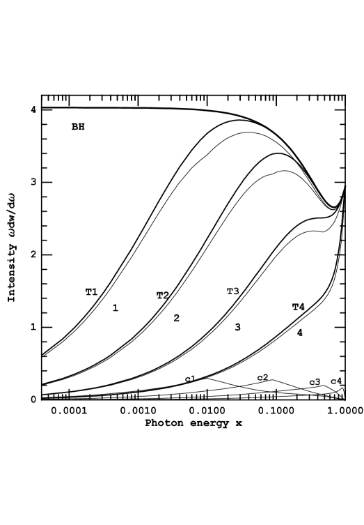
Figure 1: The spectral intensity of radiation $\omega dW/d\omega=xdW/dx,~{}x=\omega/\varepsilon$ in gold in terms of $3L_{rad}$ taken with the Coulomb corrections. Curve BH is the Bethe-Maximon spectral intensity (see Eq.(29)); curve 1 is the logarithmic approximation $\omega dW_{c}/d\omega$ Eq.(19), curve c1 is the first correction to the spectral intensity $\omega dW_{1}/d\omega$ Eq.(22) and curve T1 is the sum of the previous contributions for the electron energy $\varepsilon=25$ GeV; curves 2, c2, T2 are the same the electron energy $\varepsilon=250$ GeV; curves 3, c3, T3 are the same for the electron energy $\varepsilon=2.5$ TeV; curves 4, c4, T4 are the same for the electron energy $\varepsilon=25$ TeV.

For relatively low energies $\varepsilon=25~{}$GeV and $\varepsilon=8~{}$GeV used in famous SLAC experiment [7], [8] we have analyzed the soft part of spectrum, including all the accompanying effects: the boundary photon emission, the multiphoton radiation and influence of the polarization of the medium (see below). The perfect agreement of the theory and data was achieved in the whole interval of measured photon energies (200 keV$\leq\omega\leq$500 MeV), see below and the corresponding figures in [5], [9], [10]. It should be pointed out that both the correction term with $F(\nu)$ and the Coulomb corrections have to be taken into account for this agreement.

When a scattering is weak ($\nu_{1}\ll 1$), the main contribution in (22) gives a region where $z\ll 1$. Then

$$\displaystyle{-{\rm Im}~{}F(\nu)={\rm Im}~{}\nu^{2}\left(R_{2}-R_{1}\right)/9,\quad L_{c}\rightarrow L_{1}},$$

$$\displaystyle{\Phi(\nu)\simeq\nu^{2}\left(R_{1}+2R_{2}\right)/6,\quad(|\nu|\ll 1)}$$ (28)

Combining the results obtained in (28) we obtain the spectral distribution of the probability of radiation in the case when scattering is weak $(|\nu|\ll 1)$

$$\frac{dW}{d\omega}=\frac{dW_{c}}{d\omega}+\frac{dW_{1}}{d\omega}=\frac{4Z^{2}\alpha^{3}n_{a}}{3m^{2}\omega}\Big{[}\frac{\omega^{2}}{\varepsilon^{2}}\big{(}\ln\left(183Z^{-1/3}\right)$$

$$\displaystyle{-\frac{1}{6}-f(Z\alpha)\big{)}+2\left(1+\frac{\varepsilon^{{}^{\prime}2}}{\varepsilon^{2}}\right)\left(\ln\left(183Z^{-1/3}\right)+\frac{1}{12}-f(Z\alpha)\right)\Big{]}},$$ (29)

where $L_{1}$ is defined in (16). This expression coincide with the known Bethe-Maximon formula for the probability of bremsstrahlung from high-energy electrons in the case of complete screening (if one neglects the contribution of atomic electrons) written down within power accuracy (omitted terms are of the order of powers of $\displaystyle{1/\gamma}$) with the Coulomb corrections, see e.g. Eq.(18.30) in [11].

At $\nu_{0}\gg 1$ the function ${\rm Im}~{}F(\nu)$ Eq.(22) has the form

$${-{\rm Im}~{}F(\nu)=\pi R_{1}/4+\nu_{0}\left(\ln 2-C+\pi/4\right)R_{2}/\sqrt{2}}.$$ (30)

Under the same conditions ($\nu_{0}\gg 1$) the function ${\rm Im}~{}\Phi(\nu)$ (19) is

$${\rm Im}~{}\Phi(\nu)=\pi R_{1}/4+\nu_{0}R_{2}/\sqrt{2}\rightarrow\nu_{0}R_{2}/\sqrt{2}.$$ (31)

So, in the region where the LPM effect is strong the probability (19) can written as

$$\frac{dW_{c}}{d\omega}=\frac{\alpha R_{2}}{\varepsilon^{2}}\left(\frac{Z^{2}\alpha^{2}\varepsilon\varepsilon^{\prime}n_{a}}{\pi\omega}L(\varrho_{c})\right)^{1/2}.$$ (32)

This means that in this limit the emission probability is proportional to the square root of the density. This fact was pointed out by Migdal [2] (see Eq.(52)).

Thus, at $\nu_{0}\gg 1$ the relative contribution of the first correction $\displaystyle{\frac{dW_{1}}{d\omega}}$ is defined by

$$r=dW_{1}/dW_{c}=\left(\ln 2-C+\pi/4\right)/2L(\varrho_{c})\simeq 0.451/L(\varrho_{c}),$$ (33)

where $\displaystyle{L(\varrho_{c})=\ln\frac{a_{s2}^{2}}{\lambda_{c}^{2}\varrho_{c}^{2}}}$. In this expression the value $r$ with the accuracy up to terms $\sim 1/L_{1}^{2}$ doesn’t depend on the energy:$L_{c}\simeq L_{1}+\ln(\varepsilon/\varepsilon_{e})/2$. Hence we can find the correction to the total probability at $\varepsilon\gg\varepsilon_{e}$. The maximal value of the correction is attained at $\varepsilon\sim 10\varepsilon_{e}$, it is $\sim 6\%$ for heavy elements.

3 Target of finite thickness

3.1 Boundary effects for a thick target

For the homogeneous target of finite thickness $l$ the radiation process in a medium depends on interrelation between $l$ and formation length $l_{f0}$ (1). In the case when $l\gg l_{f0}$ we have the thick target where radiation on the boundary should be incorporated. In the case when $l\ll l_{f0}$ we have the thin target where the mechanism of radiation is changed essentially and in the case when $l\sim l_{f0}$ we have intermediate thickness.

The spectral distribution of the probability of radiation of boundary photons can be written in the form [5]

$$\frac{dw_{b}}{d\omega}=\frac{4\alpha}{\omega}{\rm Re}\left<0|r_{1}M+r_{2}{\bf p}M{\bf p}|0\right>,\quad M=\left(\frac{1}{H+\kappa}-\frac{1}{{\bf p}^{2}+1}\right)^{2},$$ (34)

where $\kappa=1+\kappa_{0}^{{}^{\prime}2},~{}\kappa_{0}^{{}^{\prime}2}=\kappa_{0}^{2}\varepsilon^{\prime}/\varepsilon,~{}\kappa_{0}=\omega_{p}/\omega,~{}\omega_{p}=\omega_{0}\gamma,~{}\omega_{0}^{2}=4\pi\alpha n_{e}/m,~{}n_{e}$ is the electron density, $\omega_{0}$ is the plasma frequency, $H$ is defined in Eq.(5), $r_{1}=R_{1}\varepsilon^{\prime}/\varepsilon=\omega^{2}/\varepsilon^{2}$,  $r_{2}=R_{2}\varepsilon^{\prime}/\varepsilon=1+\varepsilon^{{}^{\prime}2}/\varepsilon^{2}$, the parameter $\kappa_{0}$ describes the polarization of medium.

In the case when both the LPM effect and effect of polarization of a medium are weak one can decompose combination in $M$ in (34)

$$\frac{1}{H+\kappa}-\frac{1}{{\bf p}^{2}+1}\simeq\frac{1}{{\bf p}^{2}+1}(iV-\kappa_{0}^{{}^{\prime}2})\frac{1}{{\bf p}^{2}+1}.$$ (35)

In the case when $\nu_{1}\ll\kappa_{0}^{2}\geq 1$ one can omit the potential $V$ in $H$ (34), so that the effect of polarization of a medium is essential, then

$$\frac{dw_{b}}{d\omega}=\frac{4\alpha}{\omega(2\pi)^{2}}\int\left<0|r_{1}M+r_{2}{\bf p}M{\bf p}|0\right>d^{2}p$$

$$=\frac{\alpha}{\pi\omega}\left\{r_{1}\left(1+\frac{1}{\kappa}-\frac{2}{\kappa-1}\ln\kappa\right)+r_{2}\left[\left(1+\frac{2}{\kappa-1}\right)\ln\kappa-2\right]\right\}$$ (36)

This result is the quantum generalization of the transition radiation probability.

3.2 A thin target

This is a situation when the formation length of radiation is much larger than the thickness $l$ of a target [9]

$$l\ll l_{f}=l_{f0}/\zeta,\quad\zeta=1+\gamma^{2}\vartheta^{2},\quad T=l/l_{f0}\ll 1/\zeta,$$ (37)

where $l_{f0}$ are defined in Eq.(1). In the case $\kappa T\ll 1$ the radiated photon is propagating in the vacuum and one can neglect the polarization of a medium. The spectral distribution of the probability of radiation from a thin target is

$$dw_{th}/d\omega=\alpha/\pi^{2}\omega\int d^{2}\varrho\left[r_{1}K_{0}^{2}(\varrho)+r_{2}K_{1}^{2}(\varrho)\right]\left(1-\exp(-V(\varrho)T)\right),$$ (38)

where $V(\varrho)$ is defined in (5), (6), $K_{n}$ is the modified Bessel function.

3.3 Multiphoton effects in energy loss spectra

It should be noted that in the experiments [7],[8] the summary energy of all photons radiated by a single electron is measured. This means that besides mentioned above effects there is an additional ”calorimetric” effect due to the multiple photon radiation. This effect is especially important in relatively thick used targets. Since the energy losses spectrum of an electron is actually measured, which is not coincide in this case with the spectrum of photons radiated in a single interaction, one have to consider the distribution function of electrons over energy after passage of a target [10].

We consider the spectral distribution of the energy losses. After summing over $n$ the probability of the successive radiation of $n$ soft photons with energies $\omega_{1},\omega_{2},\ldots\omega_{k}$ by a particle with energy $\varepsilon~{}(\omega_{k}\ll\varepsilon,k=1,2\dots n)$ under condition $\sum_{k=1}^{n}\omega_{k}=\omega$ on the length $l$ in the energy intervals $d\omega_{1}d\omega_{2}\ldots d\omega_{n}$ we obtain [10]

$$\frac{d\varepsilon}{d\omega}=\frac{1}{\pi}~{}{\rm Re}\int_{0}^{\infty}\exp\left(ix\right)\exp\left\{-\int_{0}^{\infty}\frac{dw}{d\omega_{1}}\left[1-\exp\left(-ix\frac{\omega_{1}}{\omega}\right)\right]d\omega_{1}\right\}dx$$ (39)

The formula (39) was derived by Landau [12] (see also [1]) as solution of the kinetic equation under assumption that energy losses are much smaller than particle’s energy (the paper [12] was devoted to the ionization losses). The energy losses are defined by the hard part of the radiation spectrum. In the soft part of the energy losses spectrum (39) the probability of radiation of one hard photon only is taken into account accurately. So,it is applicable for the thin targets only and has an accuracy $l/L_{rad}$.

We will analyze first the interval of photon energies where the Bethe-Maximon formula is valid. Substituting this formula for $dw/d\omega$ (within the logarithmic accuracy) into Eq.(39) we have

$$\frac{d\varepsilon}{d\omega}=\beta f_{BM},~{}f_{BM}=\frac{\exp(-\beta\mu)}{\Gamma(1+\beta)},~{}\beta=\frac{4l}{3L_{rad}},~{}\mu=\ln\frac{\varepsilon}{\omega}-\frac{5}{8}+C,$$ (40)

where $\Gamma(z)$ is the Euler gamma function. If we consider radiation of the one soft photon, we have from (39) $d\varepsilon/d\omega=\beta$. Thus, the formula (40) gives additional ”reduction factor” $f_{BM}$ which characterizes the distortion of the soft Bethe-Maximon spectrum due to multiple photons radiation. The emission of accompanying photons with energy much lesser or of the order of $\omega$ changes the spectral distribution on quantity order of $\beta$. However, if one photon with energy $\omega_{r}>\omega$ is emitted, at least, then photon with energy $\omega$ is not registered at all in the corresponding channel of the calorimeter. Since mean number of photons with energy larger than $\omega$ is determined by the expression

$$\sum_{n=0}^{\infty}nw_{n}=w_{\omega}=\int_{\omega}^{\varepsilon}(dw/d\omega)~{}d\omega,$$ (41)

where $w_{n}$ is the probability of radiation of $n$ soft photons. So, when radiation is described by the Bethe-Maximon formula the value $w_{\omega}$ increases as a logarithm with $\omega$ decrease ($w_{\omega}\simeq\beta\ln\varepsilon/\omega$) and for large ratio $\varepsilon/\omega$ the value $w_{\omega}$ is much larger than $\beta$. Thus, amplification of the effect is connected with a large interval of the integration ($\omega\div\varepsilon$) at evaluation of the radiation probability.

If we want to improve accuracy of the formula (39) and for the case of thick targets $l\geq L_{rad}$ one has to consider radiation of an arbitrary number of hard photons. This problem is solved in Appendix of [10] for the case when hard part of the radiation spectrum is described by the Bethe-Maximon formula. In this case the formula (39) acquires the additional factor. As a result we extend this formula on the case thick targets.

The Bethe-Maximon formula becomes inapplicable for the photon energies $\omega\leq\omega_{c}$, where LPM effect starts to manifest itself (see Eq.(27)). Calculating the integral in (39) we find for the distribution of the spectral energy losses

$$\frac{d\varepsilon}{d\omega}=3\beta\sqrt{\frac{\omega}{2\omega_{c}}}f_{LPM},\quad f_{LPM}=\left(1+\frac{3\pi}{2\sqrt{2}}\beta\sqrt{\frac{\omega}{\omega_{c}}}\right)\exp(-w_{c}),$$ (42)

where $f_{LPM}$ is the reduction factor in the photon energy range where the LPM effect is essential,

$$w_{c}=\beta\left(\ln\varepsilon/\omega_{c}+C_{2}\right),\quad C_{2}\simeq 1.959.$$ (43)

In this expression the terms $\sim 1/L$ (see Sec.2) are not taken into account.

In the region $\omega\ll\omega_{p}$ (see Eq.(34)) where the contribution of boundary photons dominates the reduction factor for transition radiation $f_{tr}$ was found in [10].

3.4 Discussion of theory and experiment

Here we compare the experimental data [7],[8] with theory predictions. According to Eq.(27) the LPM effect becomes significant for $\omega\leq\omega_{c}=\varepsilon^{2}/\varepsilon_{e}$. The mechanism of radiation depends strongly on the thickness of the target. The thickness of used target in terms of the formation length is

$$\displaystyle{\beta(\omega)\equiv\frac{l}{l_{f}(\omega)}=T\left(\nu_{0}+\kappa\right)\simeq T_{c}\left[\frac{\omega}{\omega_{c}}+\sqrt{\frac{\omega}{\omega_{c}}}+\frac{\omega_{p}^{2}}{\omega\omega_{c}}\right]},$$

$$\displaystyle{T=\frac{l\omega}{2\gamma^{2}},\quad\omega_{p}=\omega_{0}\gamma,\quad T_{c}\equiv T(\omega_{c})\simeq\frac{2\pi}{\alpha}\frac{l}{L_{rad}}},$$ (44)

where we put that $\displaystyle{\nu_{0}\simeq\sqrt{\frac{\omega_{c}}{\omega}}}$ (see Eq.(26)). Below we assume that $\omega_{c}\gg\omega_{p}$ which is true under the experimental conditions. So we have that

$$T_{c}=2\pi l/\alpha L_{rad}\geq 20\quad{\rm at}\quad l/L_{rad}\geq 2~{}\%.$$ (45)

For $T_{c}\gg 1$ ($\beta(\omega_{c})\gg 1$) the minimal value of the ratio of the thickness of a target to the formation length follows from Eq.(44):$\beta_{m}\simeq 2T_{c}(\omega_{p}/\omega_{c})^{2/3}$ and is attained for the heavy elements (Au, W, U) at the initial energy $\varepsilon=25$ GeV. In this case one has $\omega_{c}\simeq 250$ MeV, $\omega_{p}\simeq 4$ MeV, $\beta_{m}\geq 2.5$.

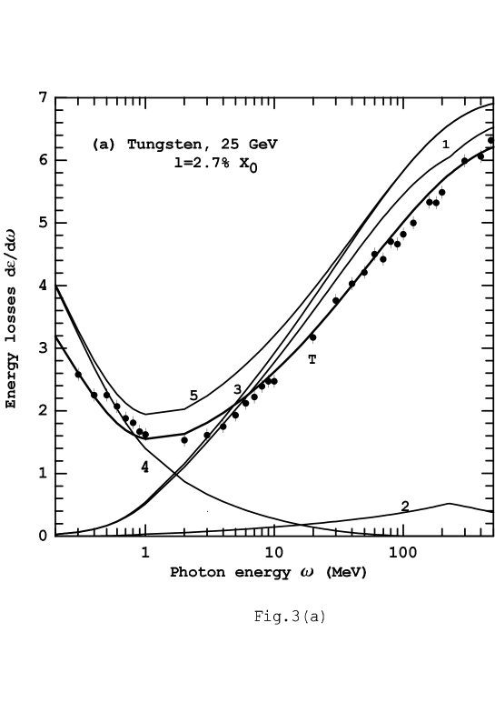
Figure 2: The energy losses $\omega dW/d\omega$ in gold with thickness $l=0.023~{}mm$ in units $2\alpha/\pi$. Curve 1 is the main (Migdal) contribution, curve 2 is the correction term, curve 3 is the sum of previous contributions, curve 4 is the contribution of boundary photons, curve 5 is the sum of the previous contributions. curve T is the final theory prediction with regard to the reduction factor (the multiphoton effects).

As an example we calculated the spectrum of the energy losses in the tungsten target with thickness $l=0.088$ mm (=$2.5~{}\%L_{rad}$) for $\varepsilon$=25 GeV. The result is shown in Fig.2. We calculated the main (Migdal type) term Eq.(19), the first correction term Eq.(22) taking into account an influence of the polarization of a medium, as well as the Coulomb corrections entering into parameter $\nu_{0}$ Eq.(24) and value $L(\varrho_{c})$ Eq.(14). We calculated also the contribution of boundary photons (see Eq.(4.12) in [5]). Here in the soft part of the spectrum $\omega<\omega_{d}~{}(\omega_{d}\simeq 2$ MeV ) the transition radiation term Eq.(36) dominates, while in the harder part of the boundary photon spectrum $\omega>\omega_{d}$ the terms depending on both the multiple scattering and the polarization of a medium give the contribution. All the mentioned contribution presented separately in Fig.2. Under conditions of the experiment the multiphoton reduction of the spectral curve is very essential. It is taken into account in the curve ”T”. Experimental data are taken from [7]. It is seen that there is a perfect agreement of the curve T with data.

4 Conclusion

The LPM effect is essential at very high energies. It will be important in electromagnetic calorimeters in TeV range. Another possible application is air showers from the highest energy cosmic rays. Let us find the lower bound of photon energy starting from which the LPM effect will affect substantially the shower development. The interaction of photon with energy lower than this bound moving vertically towards earth surface will be described by standard (Bethe-Maximon) formulas. The probability $w_{p}(h)$ to find the primary photon on the altitude $h$ is

$$dw_{p}/dh=w_{p}\exp(-h/h_{0})/l_{p},~{}w_{p}(h)=\exp\left(-h_{0}e^{-h/h_{0}}/l_{p}\right),$$ (46)

where $l_{p}\simeq 9l_{r}/7,~{}l_{r}$ is the radiation length on the ground level ($l_{r}\simeq$ 0.3 km), $h_{0}\simeq 8.7~{}$ km. The parameter $\nu_{p}^{2}$ (see Eq.(26)) characterizing the maximal strength of the LPM effect at pair creation by a photon $(\varepsilon_{+}=\varepsilon_{-}=\omega/2)$ has a form

$$\nu_{p}^{2}=(\omega/\omega_{e})\exp(-h/h_{0})w_{p}(h)=(\omega/\omega_{e})\exp(-h_{0}e^{-h/h_{0}}/l_{p}-h/h_{0}),$$ (47)

where $\omega_{e}$ is the characteristic critical energy for air on the ground level ($\omega_{e}=4\varepsilon_{e}\simeq 10^{18}$ eV). The last expression has a maximum at $h_{m}=h_{0}\ln(h_{0}/l_{p})$, so that $\nu_{p}^{2}(h_{m})=\omega/\omega_{m},~{}\omega_{m}=\omega_{e}h_{0}e/l_{p}\simeq 6\cdot 10^{19}$eV. Bearing in mind that the LPM effect becomes essential for photon energy order of magnitude higher than $\omega_{m}$ (e.g. the probability of pair creation is half of Bethe-Maximon value at $\omega=12\omega_{e}$) we have that the LPM effect becomes essential for shower formation for photon energy $\omega\simeq 5\cdot 10^{20}$ eV. It should be noted that GZK cutoff for proton is $5\cdot 10^{19}$ eV. So the the photons with the mentioned energy are extremely rare.

References

- [1] L. D. Landau and I. Ya. Pomeranchuk, Dokl.Akad.Nauk SSSR 92, 535, 735 (1953). See in English in The Collected Papers of L. D. Landau, Pergamon Press, 1965.
- [2] A. B. Migdal, Phys. Rev. 103, 1811 (1956).
- [3] V.N.Baier, V.M.Katkov and V.M.Strakhovenko, Sov. Phys. JETP 67, 70 (1988).
- [4] V.N.Baier, V.M.Katkov and V.M.Strakhovenko, Electromagnetic Processes at High Energies in Oriented Single Crystals, World Scientific Publishing Co, Singapore, 1998.
- [5] V. N. Baier and V. M. Katkov, Phys.Rev. D57, 3146 (1998).
- [6] V. N. Baier and V. M. Katkov, Phys.Rev. D62, 036008 (2000).
- [7] P. L. Anthony, R. Becker-Szendy, P. E. Bosted et al, Phys.Rev.D56, 1373 (1997).
- [8] S.Klein, Rev. Mod. Phys. 71, 501 (1999).
- [9] V. N. Baier and V. M. Katkov, Quantum Aspects of Beam Physics, ed.P. Chen, World Scientific PC, Singapore, 1998, p.525.
- [10] V. N. Baier and V. M. Katkov, Phys.Rev. D59, 056003 (1999).
- [11] V. N. Baier, V. M. Katkov and V. S Fadin, Radiation from Relativistic Electrons (in Russian) Atomizdat, Moscow, 1973.
- [12] L. D. Landau J.Phys. USSR 8 (1944) 201.