The MSW effect and Solar Neutrinos

A. Yu. Smirnov^2,3

(2) The Abdus Salam International Centre for Theoretical Physics, I-34100 Trieste, Italy
(3) Institute for Nuclear Research of Russian Academy of Sciences, Moscow 117312, Russia

The MSW (Mikheyev-Smirnov-Wolfenstein) effect is the effect of transformation of one neutrino species (flavor) into another one in a medium with varying density. Three basic elements of the effect include: the refraction of neutrinos in matter, the resonance (level crossing) and the adiabaticity. The key notion is the neutrino eigenstates in matter. Physical picture of the effect is described in terms of the flavors and the relative phases of eigenstates and the transitions between eigenstates. Features of the large mixing realization of the MSW effect are discussed. The large mixing MSW effect (LMA) provides the solution of the solar neutrino problem. We show in details how this mechanism works. Physics beyond the LMA solution is discussed. The lower $Ar$-production rate (in comparison with the LMA prediction) and absence of significant turn up of the spectrum at low energies can be due to an additional effect of the light sterile neutrino with very small mixing.

1 Introduction

1.1 Context

The key components of the context in which the mechanism of resonance flavor conversion has been proposed include

• Neutrino mixing and oscillations invented by B. Pontecorvo (1957, 1958) (neutrino-antineutrino oscillations, maximal mixing) [1] and $\nu_{e}-\nu_{\mu}$ (flavor) mixing as well as the “virtual $\nu_{e}-\nu_{\mu}$ transmutation” proposed by Z. Maki, M. Nakagawa, S. Sakata [2] (1962).

• Spectroscopy of solar neutrinos: the program put forward by J. N. Bahcall [3] and independently by G. Zatsepin and V. Kuzmin [4] to study interior of the Sun by measuring fluxes of all components of the solar neutrino spectrum. It was proposed to perform several experiments with different energy thresholds.

• The results of the Homestake experiment [5]: they led to formulation of the solar neutrino problem which has triggered major experimental and theoretical developments in neutrino physics in the last 30 years. In fact, the problem was predicted by B. Pontecorvo [6], who also suggested its vacuum oscillation solution [6, 7] (averaged vacuum oscillations with maximal or near maximal mixing).

• Matter effects on neutrino oscillations introduced by L. Wolfenstein [8].

1.2 References

Here I give (with some comments) references to the early papers on the MSW effect written by W.[8, 9, 10] and M.-S.[11, 12, 13, 14].

L. Wolfenstein:
[1] “Neutrino oscillations in matter”, Phys. Rev. D17:2369-2374, 1978. Topics include: neutrino refraction, mixing in matter, eigenstates for propagation in matter, evolution equation, modification of vacuum oscillations.

[2] “Effect of Matter on Neutrino Oscillations”, in “Neutrino -78”, Purdue Univ. C3 - C6, 1978. The adiabatic formula has been given for massless neutrino conversion in varying density.

[3] “Neutrino oscillations and stellar collapse”, Phys. Rev. D20:2634-2635, 1979. Suppression of oscillations in matter of the star is emphasized.

We started to work in the beginning of 1984, when Stas Mikheyev had shown me the Wolfenstein’s paper [1]. The question was about validity of the results and necessity to use them in the oscillation analysis of the atmospheric neutrino data from the Baksan telescope.

S.P. Mikheev, A.Yu. Smirnov:
[4] “Resonant amplification of neutrino oscillations in matter and spectroscopy of solar neutrinos”, Yad. Fiz. 42:1441-1448, 1985 [Sov.J. Nucl. Phys. 42:913-917, 1985.]
[5] “Resonant amplification of neutrino oscillations in matter and solar neutrino spectroscopy”, Nuovo Cim. C9:17-26, 1986. Appearance of these two papers with very close but not identical content (e.g., in [5] we comment on the effect in the three neutrino context) is a result of problems with publications.

[6] “Neutrino oscillations in a variable density medium and neutrino bursts due to gravitational collapse of stars”, Zh. Eksp. Teor. Fiz.91:7-13, 1986, [Sov. Phys. JETP 64:4-7,1986.]. Theory of the adiabatic neutrino conversion is presented. Here formulas for adiabatic probabilities can be found. To “cheat” editors and referees and to avoid a fate of previous papers we have removed the term “resonance” and “solar neutrinos” as well as references to our previous papers [4] [5]. The paper had been submitted to JETP Letters in the fall of 1985 and successfully … rejected. It has been resubmitted to JETP in December of 1985. The theory is applied, of course, to solar neutrinos and the paper was reprinted in “Solar Neutrinos: The first Thirty Years”, Ed. J. N. Bahcall, et al., Addison-Wesley 1995.

[7] “Neutrino oscillations in Matter with Varying density”, Proc. of the 6th Moriond Workshop on Massive Neutrinos in Astrophysics and Particle Physics (Tignes, Savoie, France) January 25 - February 1, 1986, eds. O. Fackler and J. Tran Thanh Van, p. 355 - 372. In two talks at Moriond, I have summarized all our results (excluding solar neutrinos) obtained in 1985. The paper contains (apart from theory of the adiabatic conversion) calculations of the Earth matter effect on the solar and atmospheric neutrinos, the graphic representation of oscillations and adiabatic conversion, some attempts to apply the matter effects to neutrinos in the Early Universe etc..

One important contribution both to physics of effect and to its promotion: in Summary talk of Savonlinna workshop, where our results have been presented for the first time, N. Cabibbo [15] has given interpretation of the effect in terms of eigenvalues and level crossing phenomenon (complementary to our description in terms of eigenstates). A possibility of such an interpretation was mentioned before by V. Rubakov (private communication) and later has been developed independently by H. Bethe [16].

What was in between 1979 and 1985? Several papers has been published on neutrino oscillations in matter with constant density [17, 18, 19, 20, 21]. In particular, in the paper by V. Barger et al, [17] and S. Pakvasa [18], it was shown that matter can enhance oscillations and for certain energy the mixing can become maximal. Furthermore, matter distinguishes neutrinos and antineutrinos and resolves the ambiguity in the sign of $\Delta m^{2}$. In [21] the index of refraction of neutrinos has been derived for moving and polarized medium, correct sign of the matter potential obtained.

2 Flavors, masses, mixing and oscillations

2.1 Introducing mixing

The flavor neutrino states: $\nu_{f}=(\nu_{e},\nu_{\mu},\nu_{\tau})$ are defined as the states which correspond to certain charge leptons: $e$, $\mu$ and $\tau$. The correspondence is established by interactions: $\nu_{l}$ and $l$ ($l=e,\mu,\tau$) interact in pairs, forming the charged currents. It is not excluded that additional neutrino states, the sterile neutrinos, $\nu_{s}$, exist. The neutrino mass states, $\nu_{1}$, $\nu_{2}$, and $\nu_{3}$, with masses $m_{1}$, $m_{2}$, $m_{3}$ are the eigenstates of mass matrix as well as the eigenstates of the total Hamiltonian in vacuum.

The vacuum mixing means that the flavor states do not coincide with the mass eigenstates. The flavor states are combinations of the mass eigenstates:

$$\nu_{l}=U_{li}\nu_{i},~{}~{}~{}l=e,\mu,\tau,~{}~{}~{}i=1,2,3,$$ (1)

where the mixing parameters $U_{li}$ form the P-MNS mixing matrix.

In the case of two neutrino mixing $\nu_{e}-\nu_{a}$, where $\nu_{a}$ is the non-electron neutrino state, we can write:

$$\nu_{e}=\cos\theta~{}\nu_{1}+\sin\theta~{}\nu_{2},~{}~{}\nu_{a}=\cos\theta~{}\nu_{2}-\sin\theta~{}\nu_{1}.$$ (2)

Here $\theta$ is the vacuum mixing angle. In the three neutrino context $\nu_{e}$ mixes with $\nu_{a}$ in the mass eigenstates $\nu_{1}$ and $\nu_{2}$ relevant for the solar neutrinos, and $\nu_{a}$ is maximal or nearly maximal mixture of $\nu_{\mu}$ and $\nu_{\tau}$.

2.2 Two aspects of mixing. Portrait of electron neutrino

There are two important physical aspects of mixing. According to (2) the flavor neutrino states are combinations of the mass eigenstates. One can think in terms of wave packets. Propagation of $\nu_{e}$ ($\nu_{a}$) is described a system of two wave packets which correspond to $\nu_{1}$ and $\nu_{2}$.

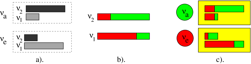
Figure 1: a). Representation of the flavor neutrino states as the combination of the mass eigenstates. The length of the box gives the admixture of (or probability to find) corresponding mass state in a given flavor state. (The sum of the lengths of the boxes is normalized to 1. b). Flavor composition of the mass eigenstates. The electron flavor is shown by red (dark) and the non-electron flavor by green (grey). The sizes of the red and green parts give the probability to find the electron and non-electron neutrino in a given mass state. c). Portraits of the electron and non-electron neutrinos: shown are representations of the electron and non-electron neutrino states as combinations of the eigenstates for which, in turn, we show the flavor composition.

In fig. 1a). we show representation of $\nu_{e}$ and $\nu_{a}$ as the combination of mass states. The lengths of the boxes, $\cos^{2}\theta$ and $\sin^{2}\theta$, give the admixtures of $\nu_{1}$ and $\nu_{2}$ in $\nu_{e}$ and $\nu_{a}$.

The key point is that the flavor states are coherent mixtures (combinations) of the mass eigenstates. The relative phase or phase difference of $\nu_{1}$ and $\nu_{2}$ in, $\nu_{e}$ and $\nu_{a}$ is fixed: according to (2) it is zero in $\nu_{e}$ and $\pi$ in $\nu_{a}$. Consequently, there are certain interference effects between $\nu_{1}$ and $\nu_{2}$ which depend on the relative phase.

The relations (2) can be inverted:

$$\nu_{1}=\cos\theta~{}\nu_{e}-\sin\theta~{}\nu_{a},~{}~{}\nu_{2}=\cos\theta~{}\nu_{a}+\sin\theta~{}\nu_{e}.$$ (3)

They determine the flavor composition of the mass states (eigenstates of the Hamiltonian), or shortly, the flavors of eigenstates. According to (3) a probability to find the electron flavor in $\nu_{1}$ is given by $\cos^{2}\theta$, whereas the probability that $\nu_{1}$ appears as $\nu_{a}$ equals $\sin^{2}\theta$. This flavor decomposition is shown in fig. 1b). by colors.

Inserting the flavor decomposition of mass states in the representation of the flavors states, we get the “portraits” of the electron and non-electron neutrinos fig. 1c). According to this figure, $\nu_{e}$ is a system of the two mass eigenstates which in turn have a composite flavor. On the first sight the portrait has a paradoxical feature: there is the non-electron (muon and tau) flavor in the electron neutrino! The paradox has a simple resolution: in the $\nu_{e}$- state the $\nu_{a}$-components of $\nu_{1}$ and $\nu_{2}$ are equal and have opposite phases. Therefore they cancel each other and the electron neutrino has pure electron flavor as it should be. The key point is interference: the interference of the non-electron parts is destructive in $\nu_{e}$. The electron neutrino has a “latent” non-electron component which can not be seen due to particular phase arrangement. However during propagation the phase difference changes and the cancellation disappears. This leads to an appearance of the non-electron component in propagating neutrino state which was originally produced as the electron neutrino. This is the mechanism of neutrino oscillations. Similar consideration holds for the $\nu_{a}$ state.

2.3 Neutrino oscillation in vacuum

In vacuum the neutrino mass states are the eigenstates of the Hamiltonian. Therefore dynamics of propagation has the following features:

• Admixtures of the eigenstates (mass states) in a given neutrino state do not change. In other words, there is no $\nu_{1}\leftrightarrow\nu_{2}$ transitions. $\nu_{1}$ and $\nu_{2}$ propagate independently. The admixtures are determined by mixing in a production point (by $\theta$, if pure flavor state is produced).

• Flavors of the eigenstates do not change. They are also determined by $\theta$. Therefore the picture of neutrino state (fig. 1c) does not change during propagation.

• Relative phase (phase difference) of the eigenstates monotonously increases.

Due to difference of masses, the states $\nu_{1}$ and $\nu_{2}$ have different phase velocities

$$\Delta v_{phase}\approx\frac{\Delta m^{2}}{2E},~{}~{}~{}~{}\Delta m^{2}\equiv m_{2}^{2}-m_{1}^{2},$$ (4)

and the phase difference changes as

$$\Delta\phi=\Delta v_{phase}t.$$ (5)

The phase is the only operating degree of freedom here.

Increase of the phase leads to oscillations. Indeed, the change of phase modifies the interference: in particular, cancellation of the non-electron parts in the state produced as $\nu_{e}$ disappears and the non-electron component becomes observable. The process is periodic: when $\Delta\phi=\pi$, the interference of non-electron parts is constructive and at this point the probability to find $\nu_{\mu}$ is maximal. Later, when $\Delta\phi=2\pi$, the system returns to its original state: $\nu(t)=\nu_{e}$. The oscillation length is the distance at which this return occurs:

$$l_{\nu}=\frac{2\pi}{v_{phase}}=\frac{4\pi E}{\Delta m^{2}}.$$ (6)

The depth of oscillations is determined by the mixing angle. It is given by maximal probability to observe the “wrong” flavor $\nu_{a}$. From the fig. 1c. one finds immediately (summing up the parts with the non-electron flavor in the amplitude)

$$depth~{}~{}of~{}~{}oscillations~{}=\sin^{2}2\theta.$$ (7)

The oscillations are the effect of the phase increase which changes the interference pattern. The depth of oscillations is the measure of mixing.

3 Matter effect.

3.1 Refraction

In matter, neutrino propagation is affected by interactions. At low energies the elastic forward scattering is relevant only (inelastic scattering can be neglected) [8]. It can be described by the potentials $V_{e}$, $V_{a}$. In usual medium a difference of the potentials for $\nu_{e}$ and $\nu_{a}$ is due to the charged current scattering of $\nu_{e}$ on electrons ($\nu_{e}e\rightarrow\nu_{e}e$) [8]:

$$V=V_{e}-V_{a}=\sqrt{2}G_{F}n_{e}~{},$$ (8)

where $G_{F}$ is the Fermi coupling constant and $n_{e}$ is the number density of electrons. Equivalently, one can describe the effect of medium in terms of the refraction index:

$$n_{ref}-1=\frac{V}{p}.$$ (9)

The difference of the potentials leads to an appearance of additional phase difference in the neutrino system: $\Delta\phi_{matter}\equiv(V_{e}-V_{a})t$. The difference of potentials (or refraction indexes) determines the refraction length:

$$l_{0}\equiv\frac{2\pi}{V_{e}-V_{a}}=\frac{\sqrt{2}\pi}{G_{F}n_{e}}.$$ (10)

$l_{0}$ is the distance over which an additional “matter” phase equals $2\pi$.

In the presence of matter the Hamiltonian of system changes:

$$H_{0}\rightarrow H=H_{0}+V,$$ (11)

where $H_{0}$ is the Hamiltonian in vacuum. Correspondingly, the eigenstates and the eigenvalues change:

$$\nu_{1},~{}~{}\nu_{2}~{}~{}~{}\rightarrow~{}~{}~{}\nu_{1m},~{}~{}\nu_{2m},$$ (12)

$$\frac{m_{1}^{2}}{2E},~{}~{}\frac{m_{2}^{2}}{2E}~{}~{}\rightarrow~{}~{}H_{1m},~{}~{}H_{2m}.$$ (13)

The mixing in matter is determined with respect to the eigenstates in matter $\nu_{1m}$ and $\nu_{2m}$. Similarly to (2) the mixing angle in matter, $\theta_{m}$, gives the relation between the eigenstates in matter and the flavor states:

$$\nu_{e}=\cos\theta_{m}\nu_{1m}+\sin\theta_{m}\nu_{2m},~{}~{}\nu_{a}=\cos\theta_{m}\nu_{2m}-\sin\theta_{m}\nu_{1m}.$$ (14)

Furthermore, in matter both the eigenstates and the eigenvalues, and consequently, the mixing angle depend on matter density and neutrino energy. It is this dependence activates new degrees of freedom of the system and leads to qualitatively new effects.

3.2 Resonance. Level crossing

In fig. 2 we show dependence of the effective mixing parameter in matter, $\sin^{2}2\theta_{m}$, on ratio of the oscillation and refraction lengths:

$$x\equiv\frac{l_{\nu}}{l_{0}}=\frac{2EV}{\Delta m^{2}}\propto En_{e}$$ (15)

for two different values of vacuum mixing angle.

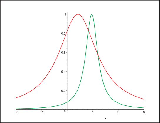
Figure 2: The dependence of the effective mixing parameter $\sin^{2}2\theta_{m}$ on the ratio $x=l_{\nu}/l_{0}$ for two different values of the vacuum mixing: $\sin^{2}2\theta=0.825$ (red) which corresponds to the LMA solution and $\tan^{2}\theta=0.08$ (green) which is at the upper bound on 1-3 mixing. The semi-plane $x<0$ corresponds to the antineutrino channel.

The dependence in fig. 2 has a resonance character. At

$$l_{\nu}=l_{0}\cos 2\theta~{}~{}~{}~{}~{}~{}~{}{\rm(resonance~{}~{}condition)}$$ (16)

the mixing becomes maximal: $\sin^{2}2\theta_{m}=1$. For small vacuum mixing the condition (16) reads:

$$Oscillation~{}~{}length\hskip 14.22636pt\approx\hskip 14.22636ptRefraction~{}~{}length.$$ (17)

That is, the eigen-frequency which characterizes a system of mixed neutrinos, $1/l_{\nu}$, coincides with the eigen-frequency of medium, $1/l_{0}$.

For large vacuum mixing (for solar LMA: $\cos 2\theta=0.4-0.5$) there is a significant deviation from the equality. Large vacuum mixing corresponds to the case of strongly coupled system for which, as usual, the shift of frequencies occurs.

The resonance condition (16) determines the resonance density:

$$n_{e}^{R}=\frac{\Delta m^{2}}{2E}\frac{\cos 2\theta}{\sqrt{2}G_{F}}~{}.$$ (18)

The width of resonance on the half of the height (in the density scale) is given by

$$2\Delta n_{e}^{R}=2n_{e}^{R}\tan 2\theta,$$ (19)

Similarly, one can introduce the resonance energy and the width of resonance in the energy scale. The width (19) can be rewritten as

$$\Delta n_{e}^{R}=n_{0}\sin 2\theta,~{}~{}~{}~{}~{}n_{0}\equiv\frac{\Delta m^{2}}{2\sqrt{2}EG_{F}}~{}.$$ (20)

When the vacuum mixing approaches maximal value, the resonance shifts to zero density: $n_{e}^{R}\rightarrow 0$, the width of the resonance increases converging to fixed value: $\Delta n_{e}^{R}\rightarrow n_{0}$.

In medium with varying density, the layer where the density changes in the interval

$$n_{e}^{R}\pm\Delta n_{e}^{R}$$ (21)

is called the resonance layer.

In fig. 3 we show dependence of the eigenvalues $H_{im}$ on the ratio $l_{\nu}/{l_{0}}$ (level crossing scheme) [15, 16]. In resonance, the level splitting is minimal and therefore the oscillation length being inversely proportional the level spitting, is maximal.

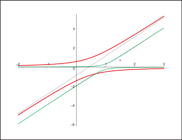
Figure 3: Level crossing scheme. Dependence of the eigenvalues of the Hamiltonian in matter, $H_{1m}$ and $H_{2m}$, on the ratio $x\equiv l_{\nu}/l_{0}$ for two different values of vacuum mixing $\sin^{2}2\theta=0.825$ (solid, blue lines) and $\sin^{2}\theta=0.08$ (dashed, red lines).

The resonance has physical meaning both for small and for large mixing. Independently of vacuum mixing in the resonance

• the flavor mixing is maximal;

• the level splitting is minimal; correspondingly, in uniform medium the oscillation length is maximal;

When the density changes on the way of neutrinos, it is in the resonance layer the flavor transition mainly occurs.

3.3 Degrees of freedom. Two effects

An arbitrary neutrino state can be expressed in terms of the instantaneous eigenstates of the Hamiltonian, $\nu_{1m}$ and $\nu_{2m}$, as

$$\nu(t)=\cos\theta_{a}\nu_{1m}+\sin\theta_{a}\nu_{2m}e^{i\phi}~{},$$ (22)

where

• $\theta_{a}=\theta_{a}(t)$ determines the admixtures of eigenstates in $\nu(t)$;
  

• $\phi(t)$ is the phase difference between the two eigenstates (phase of oscillations):

  $$\phi(t)=\int_{0}^{t}\Delta Hdt^{\prime}+\phi(t)_{T}~{},$$ (23)

  here $\Delta H\equiv H_{1m}-H_{2m}$. The integral gives the adiabatic phase and $\phi(t)_{T}$ is the rest which can be related to violation of adiabaticity. It may also have a topological contribution (Berry phase) in more complicated systems;
  

• $\theta_{m}(n_{e}(t))$ determines the flavor content of the eigenstates: $\langle\nu_{e}|\nu_{1m}\rangle=\cos\theta_{m}$, etc..

Different processes are associated with these three different degrees of freedom. In what follows we will consider two of them:

1. The resonance enhancement of neutrino oscillations which occurs in matter with constant density. It is induced by the relative phase of neutrino eigenstates.

2. The adiabatic (partially adiabatic) conversion which occurs in medium with varying density and is related to the change of mixing or flavor of the neutrino eigenstates.

In general, an interplay of the oscillations and the resonance conversion occurs.

4 The MSW effect

4.1 Oscillations in matter. Resonance enhancement of oscillations

In medium with constant density the mixing is constant: $\theta_{m}(E,n)=const$. Therefore

• The flavors of the eigenstates do not change.

• The admixtures of the eigenstates do not change. There is no $\nu_{1m}\leftrightarrow\nu_{2m}$ transitions, $\nu_{1m}$ and $\nu_{2m}$ are the eigenstates of propagation.

• Monotonous increase of the phase difference between the eigenstates occurs: $\Delta\phi_{m}=(H_{2m}-H_{1m})t$.

This is similar to what happens in vacuum. The only operative degree of freedom is the phase. Therefore, as in vacuum, the evolution of neutrino has a character of oscillations. However, parameters of oscillations (length, depth) differ from the parameters in vacuum. They are determined by the mixing in matter and by the effective energy splitting in matter:

$$\sin^{2}2\theta\rightarrow\sin^{2}2\theta_{m},~{}~{}~{}~{}~{}~{}l_{\nu}\rightarrow l_{m}=\frac{2\pi}{H_{2m}-H_{1m}}.$$ (24)

For a given density of matter the parameters of oscillations depend on the neutrino energy which leads to a characteristic modification of the energy spectra. Suppose a source produces the $\nu_{e}$- flux $F_{0}(E)$. The flux crosses a layer of length, $L$, with a constant density $n_{e}$ and then detector measures the electron component of the flux at the exit from the layer, $F(E)$.

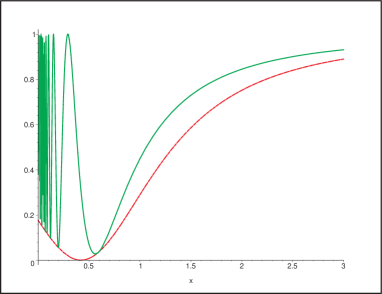
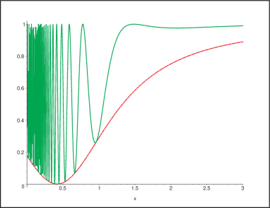
Figure 4:   Resonance enhancement of oscillations in matter with constant density. Shown is a dependence of the ratio of the final and original fluxes, $F/F_{0}$, on energy ($x\propto E$) for a thin layer, $L=l_{0}/\pi$ (left panel) and thick layer $L=10l_{0}/\pi$ (right panel). $l_{0}$ is the refraction length. The vacuum mixing equals $\sin^{2}2\theta=0.824$.

In fig. 4 we show dependence of the ratio $F(E)/F_{0}(E)$ on energy for thin and thick layers. The ratio has an oscillatory dependence. The oscillatory curve (green) is inscribed in to the resonance curve $(1-\sin^{2}2\theta_{m})$ (red). The frequency of the oscillations increases with the length $L$. At the resonance energy, the oscillations proceed with maximal depths. Oscillations are enhanced in the resonance range:

$$E=E_{R}\pm\Delta E_{R},~{}~{}~{}\Delta E_{R}=\tan 2\theta~{}E_{R}=\sin 2\theta~{}E_{R}^{0},$$ (25)

where $E_{R}^{0}=\Delta m^{2}/2\sqrt{2}G_{F}n_{e}$. Several comments: for $E\gg E_{R}$, matter suppresses the oscillation depth; for small mixing the resonance layer is narrow, and the oscillation length in the resonance is large. With increase of the vacuum mixing: $E_{R}\rightarrow 0$ and $\Delta E_{R}\rightarrow E_{R}^{0}$.

The oscillations in medium with nearly constant density are realized for neutrinos crossing the mantle of the Earth.

4.2 MSW: adiabatic conversion

In non-uniform medium, density changes on the way of neutrinos: $n_{e}=n_{e}(t)$. Correspondingly, the Hamiltonian of system depends on time: $H=H(t)$. Therefore,

(i). the mixing angle changes in the course of propagation: $\theta_{m}=\theta_{m}(n_{e}(t))$;

(ii). the (instantaneous) eigenstates of the Hamiltonian, $\nu_{1m}$ and $\nu_{2m}$, are no more the “eigenstates” of propagation: the transitions $\nu_{1m}\leftrightarrow\nu_{2m}$ occur.

However, if the density changes slowly enough (the adiabaticity condition) the transitions $\nu_{1m}\leftrightarrow\nu_{2m}$ can be neglected. This is the essence of the adiabatic condition: $\nu_{1m}$ and $\nu_{2m}$ propagate independently, as in vacuum or uniform medium. Therefore dynamical features can be summarized in the following way:

• The flavors of the eigenstates change according to density change. The flavor composition of the eigenstates is determined by $\theta_{m}(t)$.

• The admixtures of the eigenstates in a propagating neutrino state do not change (adiabaticity: no $\nu_{1m}\leftrightarrow\nu_{2m}$ transitions). The admixtures are given by the mixing in production point, $\theta_{m}^{0}$.

• The phase difference increases; the phase velocity is determined by the level splitting (which in turn, changes with density (time)).

Now two degrees of freedom become operative: the relative phase and the flavors of neutrino eigenstates. The MSW effect is driven by the change of flavors of the neutrino eigenstates in matter with varying density. The change of phase produces the oscillation effect on the top of the adiabatic conversion.

Let us comment on the adiabaticity condition. If external conditions (density) change slowly, the system (mixed neutrinos) has time to adjust this change. In general, the adiabaticity condition can be written as [22, 23]

$$\gamma=\left|\frac{\dot{\theta}_{m}}{H_{2m}-H_{1m}}\right|\ll 1.$$ (26)

As follows from the evolution equation for the neutrino eigenstates [13, 22], $|\dot{\theta}_{m}|$ determines the energy of transition $\nu_{1m}\leftrightarrow\nu_{2m}$ and $|H_{2m}-H_{1m}|$ gives the energy gap between levels. The condition (26) means that the transitions $\nu_{1m}\leftrightarrow\nu_{2m}$ can be neglected and the eigenstates propagate independently (the angle $\theta_{a}$ (22) is constant).

The adiabaticity condition is crucial in the resonance layer where (i) the level splitting is small and (ii) the mixing angle changes rapidly. If the vacuum mixing is small, the adiabaticity is critical in the resonance point. It takes the form [11]

$$\Delta r_{R}>l_{R},$$ (27)

where $l_{R}=l_{\nu}/\sin 2\theta$ is the oscillation length in resonance, and $\Delta r_{R}=n_{R}/(dn_{e}/dr)_{R}\tan 2\theta$ is the spatial width of resonance layer. According to (27) for the adiabatic evolution at least one oscillation length should be obtained in the resonance layer. The adiabaticity condition has been considered outside the resonance and in the non-resonance channel in [24].

In the case of large vacuum mixing the point of maximal adiabaticity violation [25, 26] is shifted to densities $n_{e}(av)$ larger than the resonance density: $n_{e}(av)\rightarrow n_{B}>n_{R}$. Here $n_{B}=\Delta m^{2}/2\sqrt{2}G_{F}E$ is the density at the border of resonance layer for maximal mixing.

Let us describe pattern of the adiabatic conversion. According to the dynamical conditions, the admixtures of eigenstates are determined by the mixing in neutrino production point. This mixing in turn, depends on the density in the initial point, $n_{e}^{0}$, as compared to the resonance density. Consequently, a picture of the conversion depends on how far from the resonance layer (in the density scale) a neutrino is produced.

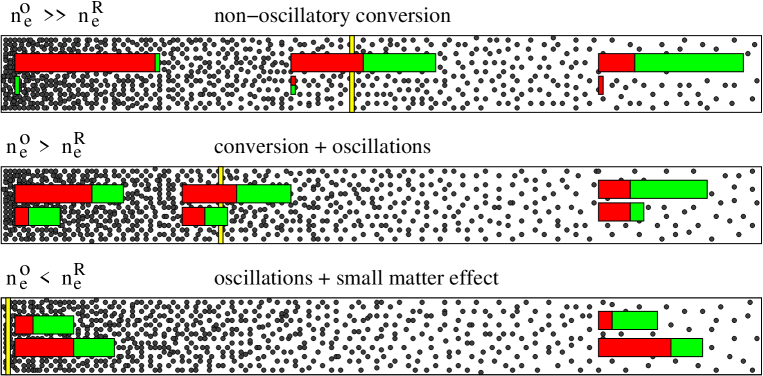
Figure 5:   Adiabatic evolution of neutrino state for three different initial condition ($n_{e}^{0}$). Shown are the neutrino states in different moments of propagation in medium with varying (decreasing) density. The yellow vertical line indicates position of resonance. The initial state is $\nu_{e}$ in all the cases. The sizes of the boxes do not change, whereas the flavors (colors) follow the density change.

Three possibilities can be identified. They are shown in fig. 5. and correspond to large vacuum mixing which is relevant for the solar neutrinos. We show propagation of the state produced as $\nu_{e}$ from large density region to zero density. Due to adiabaticity the sizes of boxes which correspond to the neutrino eigenstates do not change.

1). $n_{e}^{0}\gg n_{e}^{R}$ - production far above the resonance (the upper panel). The initial mixing is strongly suppressed, consequently, the neutrino state, $\nu_{e}$, consists mainly of one ($\nu_{2m}$) eigenstate, and furthermore, one flavor dominates in a given eigenstate. In the resonance (its position is marked by the yellow line) the mixing is maximal: both flavors are present equally. Since the admixture of the second eigenstate is very small, oscillations (interference effects) are strongly suppressed. So, here we deal with the non-oscillatory flavor transition when the flavor of whole state (which nearly coincides with $\nu_{2m}$) follows the density change. At zero density we have $\nu_{2m}=\nu_{2}$, and therefore the probability to find the electron neutrino (survival probability) equals

$$P=|\langle\nu_{e}|\nu(t)\rangle|^{2}\approx|\langle\nu_{e}|\nu_{2m}(t)\rangle|^{2}=|\langle\nu_{e}|\nu_{2}\rangle|^{2}\approx\sin^{2}\theta.$$ (28)

The value of final probability, $\sin^{2}\theta$, is the feature of the non-oscillatory transition. Deviation from this value indicates a presence of oscillations.

2). $n_{e}^{0}>n_{e}^{R}$ production above the resonance (middle panel). The initial mixing is not suppressed. Although $\nu_{2m}$ is the main component, the second eigenstate, $\nu_{1m}$, has appreciable admixture; the flavor mixing in the neutrino eigenstates is significant. So, the interference effect is not suppressed. As a result, here an interplay of the adiabatic conversion and occurs.

3). $n_{e}^{0}<n_{e}^{R}$: production below the resonance (lower panel). There is no crossing of the resonance region. In this case the matter effect gives only corrections to the vacuum oscillation picture.

The resonance density is inversely propotional to the neutrino energy: $n_{e}^{R}\propto 1/E$. So, for the same density profile, the condition 1) is realized for high energies, regime 2) for intermediate energies and 3) – for low energies. As we will see all three case are realized for solar neutrinos.

4.3 Universality

The adiabatic transformations show universality: The averaged probability and the depth of oscillations in a given moment of propagation are determined by the density in a given point and by initial condition (initial density and flavor). They do not depend on density distribution between the initial and final points. In contrast, the phase of oscillations is an integral effect of previous evolution and it depends on a density distribution.

Universal character of the adiabatic conversion can be further generalized in terms of variable [13, 14]

$$n=\frac{n_{e}^{R}-n_{e}}{\Delta n_{e}^{R}}$$ (29)

which is the distance (in the density scale) from the resonance density in the units of the width of resonance layer. In terms of $n$ the conversion pattern depend only on initial value $n_{0}$.

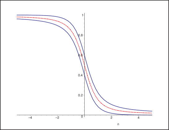
Figure 6:   The dependence of the average probability (dashed line) and the depth of oscillations ($P^{max}$, $P^{min}$ solid lines) on $n$ for $n_{0}=-5$. The resonance layer corresponds to $n=0$. For $\tan^{2}\theta=0.4$ (large mixing MSW solution) the evolution stops at $n_{f}=0.47$.

In fig. 6 we show dependences of the average probability and depth of oscillations, that is, $\bar{P}$, $P^{max}$, and $P^{min}$, on $n$. The probability itself is the oscillatory function which is inscribed into the band shown by solid lines. The average probability is shown by the dashed line. The curves are determined by initial value $n_{0}$ only, in particular, there is no explicit dependence on the vacuum mixing angle. The resonance is at $n=0$ and the resonance layer is given by the interval $n=-1\div 1$. The figure corresponds to $n_{0}=-5$, i.e., to production above the resonance layer; the oscillation depth is relatively small. With further decrease of $n_{0}$, the oscillation band becomes narrower approaching the line of non-oscillatory conversion. For zero final density we have

$$n_{f}=\frac{1}{\tan 2\theta}.$$ (30)

So, the vacuum mixing enters final condition. For the best fit LMA point, $n_{f}=0.45-0.50$, and the evolution should stop at this point. The smaller mixing the larger final $n_{f}$ and the stronger transition.

4.4 Adiabaticity violation

In the adiabatic regime the probability of transition between the eigenstates is exponentially suppressed $P_{12}\sim exp{(-\pi/2\gamma)}$ and $\gamma$ is given in (26) [27, 28]. One can consider such a transition as penetration through a barrier of the height $H_{2m}-H_{1m}$ by a system with the kinetic energy $d\theta_{m}/dt$.

If density changes rapidly, so that the condition (26) is not satisfied, the transitions $\nu_{1m}\leftrightarrow\nu_{2m}$ become efficient. Therefore admixtures of the eigenstates in a given propagating state change. In our pictorial representation (fig. 5) the sizes of boxes change. Now all three degrees of freedom of the system become operative.

Typically, adiabaticity breaking leads to weakening of the flavor transition. The non-adiabatic transitions can be realized inside supernovas for the very small 1-3 mixing.

5 Solar Neutrinos. Large Angle MSW solution

The first KamLAND result [29] has confirmed the large mixing MSW (LMA) solution of the solar neutrino problem. Both the total rate of events and the spectrum distortion are in a very good agreement with predictions made on the basis of LMA [30].

According to the large angle MSW solution, inside the Sun the initially produced electron neutrinos undergo adiabatic conversion. Adiabaticity condition is fulfilled with very high accuracy for all relevant energies. Inside the Sun several thousands of oscillation lengths are obtained.

On the way from the Sun to the Earth the coherence of neutrino state is lost and at the surface of the Earth, incoherent fluxes of the mass states $\nu_{1}$ and $\nu_{2}$ arrive. In the matter of the Earth $\nu_{1}$ and $\nu_{2}$ oscillate producing partial regeneration of the $\nu_{e}$-flux.

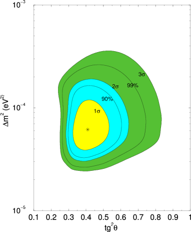
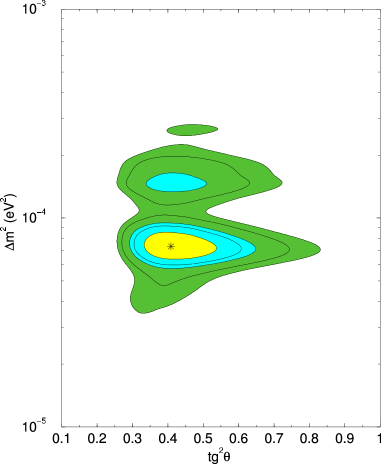
Figure 7:   The best fit points and the allowed regions (at different C.L.) of the oscillation parameters (at different C.L.) from the global fit of the solar neutrino data (left), and from the combined analysis of the solar neutrino data and KamLAND (right).

In fig. 7 from [31] we show the best fit point and the allowed regions of oscillation parameters from (a) analysis of the solar neutrino data and (b) combined analysis of the solar and KamLAND results (in assumption of the CPT invariance). The best fit point is at

$$\Delta m^{2}\sim 7\cdot 10^{-5}{\rm eV}^{2},~{}~{}~{}~{}\tan^{2}\theta\sim 0.4.$$ (31)

For these parameters, the energy “profile of the effect” - the dependence of the survival probability on the neutrino energy is shown in fig. 8. In fig. 9 we present conversion patterns for different neutrino energies.

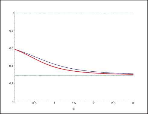
Figure 8:   Profile of the effect. Dependence of the survival probability on neutrino energy for the best fit values of parameters and production in the center of the Sun (solid line). For $\Delta m^{2}=7\cdot 10^{-5}$ eV², $x=2$ corresponds to $E\approx 10$ MeV. The dashed line shows the averaging effect over the production region $R=0.1R_{sun}$. The Earth matter regeneration effect is not included.

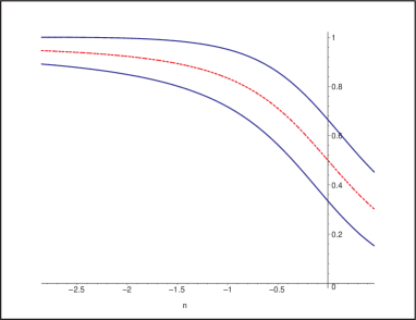
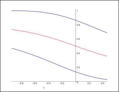
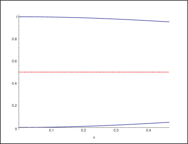
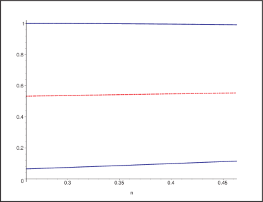
Figure 9:   The evolution of the neutrinos with different energies in the Sun. Shown are the dependences of the averaged value of the survival probability (dashed lines), as well as maximal and minimal values of the probability (solid lines) on $n$. Neutrino is produced in the center of the Sun. The density decreases from the left to the right. The resonance cis at $n=0$. The probability is the oscillatory curve which is inscribed in the band between $P^{max}$ and $P^{min}$. Upper left panel: $E=14$ MeV, upper right panel: $E=6$ MeV, lower left panel $E=2$ MeV, lower right panel $E=0.86$ MeV.

There are three energy ranges with different features of transition:

1. In the high energy part of spectrum, $E>10$ MeV ($x>2$), the adiabatic conversion with small oscillation effect occurs. The spatial evolution (in $n$-scale) is shown in the upper left panel of fig. 9. At the exit, the resulting averaged probability is slightly larger than $\sin^{2}\theta$ expected from the non-oscillatory transition. Pictorial representation of the conversion is shown in fig. 9. With decrease of energy the initial density approaches the resonance density, and the depths of oscillations increases.

2. Intermediate energy range $E\sim(2-10)$ MeV ($x=0.3-2$ ) the oscillation effect is significant. The interplay of the oscillations and conversion takes place (fig. 9).

For $E\sim 2$ MeV neutrinos are produced in resonance (bottom left panel). Initial depth of oscillations is maximal and $\bar{P}=0.5$.

3. At low energies: $E<2$ MeV ($x<0.3$), the vacuum oscillations with small matter corrections occur.

Notice that without matter effect for all energies one would get the pattern of evolution close to that in the bottom-right panel.

Basically this is what was called the “adiabatic solution” in the early days: the boron neutrino spectrum is “sitting” on the adiabatic edge of the suppression pit. An absence of observable spectrum distortion allows now only the large mixing part of the adiabatic solution.

As a specific example, let us consider neutrinos with $E=10$ MeV produced in the center of the Sun. For these neutrinos the resonance density equals $n_{R}Y_{e}=20$ g/cc, where $Y_{e}$ is the number of electrons per nucleon. The resonance layer is in the central parts of the Sun: $R_{R}=0.24R_{sun}$. In the production point: $\sin^{2}\theta_{m}=0.94$ and $\cos^{2}\theta_{m}=0.06$, so indeed, $\nu_{2m}$ dominates. At the surface of the Sun the state $\nu_{2m}$ appears as $\nu_{2}$ and then arrives at the Earth loosing the coherence with $\nu_{1}$. Entering the Earth the state $\nu_{2}$ splits in two matter eigenstates:

$$\nu_{2}\rightarrow\cos\theta_{m}^{\prime}\nu_{2m}+\sin\theta_{m}^{\prime}\nu_{1m}.$$ (32)

It oscillates regenerating the $\nu_{e}$-flux. With the Earth matter effect taken into account, the survival probability at high energies can be written as

$$P\approx\sin^{2}\theta+f_{reg},$$ (33)

where the regeneration factor equals

$$f_{reg}=0.5\sin^{2}2\theta~{}\frac{l_{\nu}}{l_{0}}~{}.$$ (34)

Notice that the oscillations of $\nu_{2}$ are pure matter effect and for the presently favored value of $\Delta m^{2}$ this effect is small. According to (34), $f_{reg}\propto 1/\Delta m^{2}$ and the expected day-night asymmetry of the charged current signal equals

$$A_{DN}=f_{reg}/P\sim(3-5)\%~{}.$$ (35)

6 Beyond LMA

Is the solar neutrino problem solved? In assumption of the CPT, the large angle MSW effect is indeed the dominant mechanism of the solar neutrino conversion, and all other possible mechanisms could give the sub-dominant effects only.

What is the next? First of all, even accepting the LMA solution one needs better determination of the oscillation parameters. In particular, further improvements of the upper bounds on $\Delta m^{2}$ and $\tan^{2}\theta$ (deviation from maximal mixing) are of great importance. These improvements have implications for both phenomenology (future long baseline experiments, double beta decay searches, etc.) and theory. The improvements are also needed for better understanding of physics of the solar neutrino conversion. In sect. 6 we have described the picture which corresponds to the oscillation parameter near the best fit point (31). Physics, in particular relative importance of the vacuum oscillations and the matter effect, changes with parameters within the presently allowed region (fig. 7).

Is large mixing MSW sufficient to describe the data? If there are observations which may indicate some deviations from LMA? According to recent analysis, LMA describes all the data very well: pulls of predictions from results of measurements are below $1\sigma$ for all but one experiment [31]). High Ar-production rate, $Q_{Ar}\sim 3$ SNU, is a generic prediction of LMA. The predicted rate is about $2\sigma$ above the Homestake result. This difference can be statistical fluctuation or some systematics which may be related to the claimed time variations of the Homestake signal.

Another generic prediction is the “turn up of spectrum” (spectrum distortion) at low energies. According to LMA the survival probability should increase with decrease of energy (fig. 8): for the best fit point the turn up can be as large as 10 - 15% between 8 and 5 MeV [31]. Neither SuperKamiokande nor SNO show any turn up although the present sensitivity is not enough to make any statistically significant statement.

Are these observations related? Do they indicate some new physics at low energies? It happens that both the lower $Ar$-production rate and absence of (or weaker) turn up of the spectrum can be explained by the effect of new (sterile) neutrino [32].

Suppose that on the top of usual pair of states with the LMA parameters (31) new light neutrino state, $\nu_{s}$, exists which

- mixes weakly with the lightest state $\nu_{1}$: $\sin^{2}2\theta_{01}\sim(10^{-4}-10^{-3})$,

- has the mass difference with $\nu_{1}$: $\Delta m^{2}_{01}=(2-10)\cdot 10^{-6}$ eV². If $\nu_{1}$ is very light, the mass of $\nu_{0}$ equals $(2-3)\cdot 10^{-3}$ eV.

It can be shown, that the presence of such a neutrino does not change the survival probability in the non-oscillatory and vacuum ranges but do change it in the transition region. In general, it leads to appearance of a dip in the adiabatic edge: at $E=(0.5-2)$ MeV and flattening of spectrum distortion at higher energies. The dip produces suppression of the $Be$-neutrino flux as well as other fluxes at the intermediate energies, and consequently, suppression of the $Ar$-production rate. It also diminishes or eliminates completely (depending on the angle and $\Delta m^{2}_{01}$) the turn up of spectrum. This scenario predicts low rate in BOREXINO: it can be as low as $\sin^{4}\theta\sim 0.1$ of the SSM rate. The scenario implies also smaller 1-2 mixing, $\tan^{2}\theta$, (to compensate decrease of the $Ge$-production rate) and larger boron neutrino flux (to reproduce the high energy data). For $\Delta m^{2}>(1-2)\cdot 10^{-5}$ eV² the turn up can be changed without diminishing the $Be$- neutrino flux.

Smallness of mixing of the sterile neutrino allows to avoid the nucleosynthesis bound: such a neutrino does not equilibrate in the Early Universe.

7 Summary

1. We have described here two matter effects:

The resonance enhancement of oscillations in matter with constant density.

The adiabatic (quasi-adiabatic) conversion in medium with varying density (MSW).

2. Adiabatic (quasi-adiabatic) conversion is related to the change of the mixing in matter on the way of neutrino, or equivalently, to the change of flavors of the neutrino eigenstates. In contrast, oscillations are related to change of the relative phase of the eigenstates.

3. The large mixing MSW effect provides the solution of the solar neutrino problem. The solar neutrino data allow to determine the oscillation parameters $\Delta m^{2}_{12}$ and $\theta_{12}$ and therefore to make next important step in reconstruction of the neutrino mass and flavor spectrum.

Now we can say how the mechanism of conversion of the solar neutrinos works. A picture of the conversion depends on neutrino energy. It has a character of

- nearly non-oscillatory transition for $E>10$ MeV,

- interplay of the adiabatic conversion and oscillations for $E=2-10$ MeV,

- oscillations with small matter corrections for $E<2$ MeV.

4. The large angle MSW effect is the dominant mechanism of the solar neutrino conversion. Although more precise determination of parameters is needed to identify completely the physical picture of the effect. All other suggested mechanisms can produce sub-leading effects. With the available data we know rather well what happens with high energy neutrinos ($E>5$ MeV). Still some physics beyond LMA may show up in the low energy part of spectrum. The low $Ar$ -production rate and absence of the turn up of the spectrum distortion in the range $E<8$ MeV can be due to an additional effect of the light sterile neutrino with very small mixing. BOREXINO [33] and KamLAND can test this possibility in future.

8 Acknowledgments

I would like to thank Milla Baldo-Ceolin for invitation to give this talk and for hospitality during my stay in Rome and Venice.

References

- [1] B. Pontecorvo, Zh. Eksp. Theor. Fiz. 33 (1957); 34 (1958) 247.
- [2] Z. Maki, M. Nakagawa and S. Sakata, Prog. Theor. Phys. 28 (1962) 870.
- [3] J. N. Bahcall, Phys. Lett. 13 332 (1964).
- [4] V. A. Kuzmin and G. T. Zatsepin Proc. of the 9th Int. Conf. on Cosmic Rays, Jaipur, India, v. 2 p. 1023 (1965).
- [5] R. Davis Jr., D.S. Harmer, K.S. Hoffman, Phys. Rev. Lett. 20, 1205, (1968).
- [6] B. Pontecorvo, ZETF, 53, 1771 (1967) [Sov. Phys. JETP, 26, 984 (1968)]
- [7] V. N. Gribov and B. Pontecorvo, Phys. Lett. 28B, 493 (1969).
- [8] L. Wolfenstein, Phys. Rev. D17 (1978) 2369.
- [9] L. Wolfenstein, in “Neutrino -78”, Purdue Univ. C3, 1978.
- [10] L. Wolfenstein, Phys. Rev. D20 2634, 1979.
- [11] S. P. Mikheyev and A. Yu. Smirnov, Sov. J. Nucl. Phys. 42 (1985) 913.
- [12] S.P. Mikheev, A.Yu. Smirnov, Nuovo Cim. C9 17, 1986.
- [13] S.P. Mikheev, A.Yu. Smirnov, Zh. Eksp. Teor. Fiz. 91, 7 (1986), [Sov. Phys. JETP 64, 4 (1986)].
- [14] S. P. Mikheyev and A. Yu. Smirnov, Proc. of the 6th Moriond Workshop on massive Neutrinos in Astrophysics and Particle Physics, Tignes, Savoie, France Jan. 1986 (eds. O. Fackler and J. Tran Thanh Van) p. 355 (1986).
- [15] N. Cabibbo, Summary talk given at 10th Int. Workshop on Weak Interactions and Neutrinos, Savonlinna, Finland, June 1985.
- [16] H. Bethe, Phys. Rev. Lett. 56, 1305 (1986).
- [17] V. Barger, K. Whisnant, S. Pakvasa and R.J. N. Phillips, Phys. Rev. D22, 2718 (1980).
- [18] S. Pakvasa, in DUMAND-80, 1981 vol.2, p.457.
- [19] H. J. Haubold, Astrophys. Spac. Sci., 82, 457 (1982).
- [20] P. V. Ramana Murthy, in Proc. of the 18th Int Cosmic Ray Conf., v. 7, 125 (1983).
- [21] P. Langacker, J. P. Leville and J. Sheiman, Phys. Rev. D 27 1228 (1983).
- [22] A. Messiah, Proc. of the 6th Moriond Workshop on Massive Neutrinos in Particle Physics and Astrophysics, eds O. Fackler and J. Tran Thanh Van, Tignes, France, Jan. 1986, p. 373.
- [23] S. P. Mikheev and A.Y. Smirnov, Sov. Phys. JETP 65, 230 (1987).
- [24] A. Yu. Smirnov, D. N. Spergel, J. N. Bahcall, Phys. Rev. D49 1389 (1994).
- [25] E. Lisi, A. Marrone, D. Montanino, A. Palazzo and S.T. Petcov, Phys. Rev. D63 093002 (2001)
- [26] A. Friedland, Phys. Rev. D64, 013008 (2001), and hep-ph/0106042.
- [27] W. C. Haxton, Phys. Rev. Lett. 57, 1271 (1986).
- [28] S. J. Parke, Phys. Rev. Lett. 57, 1275 (1986).
- [29] K. Eguchi et al, (KamLAND collaboration), Phys. Rev. Lett, 90 021802 (2003).
- [30] J. N. Bahcall, M. C. Gonzalez-Garcia, and C. Pena-Garay, JHEP 079(2002) 0054; P. C. de Holanda and A. Yu. Smirnov, Phys. Rev D66:113005, (2002).
- [31] P. C. de Holanda and A. Yu. Smirnov, JCAP 01 (2003) 001.
- [32] P. de Holanda and A. Yu. Smirnov, in preparation.
- [33] G. Alimonti et al, (BOREXINO) Astrophysics J. 16 205 (2002).