ANALYTIC INVARIANT CHARGE AND THE LATTICE STATIC QUARK–ANTIQUARK POTENTIAL

Abstract

A recently developed model for the QCD analytic invariant charge is compared with quenched lattice simulation data on the static quark–antiquark potential. By employing this strong running coupling one is able to obtain the confining quark–antiquark potential in the framework of the one–gluon exchange model. To achieve this objective a technique for evaluating the integrals of a required form is developed. Special attention is paid here to removing the divergences encountered the calculations. All this enables one to examine the asymptotic behavior of the potential at both small and large distances with high accuracy. An explicit expression for the quark–antiquark potential, which interpolates between these asymptotics, and satisfies the concavity condition, is proposed. The derived potential coincides with the perturbative results at small distances, and it is in a good agreement with the lattice data in the nonperturbative physically–relevant region. An estimation of the parameter $\Lambda_{\mbox{\tiny QCD}}$ is obtained for the case of pure gluodynamics. It is found to be consistent with all the previous estimations of $\Lambda_{\mbox{\tiny QCD}}$ in the framework of approach in hand.

Received 12 December 2003

1 Introduction

The description of hadron dynamics at large distances remains a crucial challenge of elementary particle physics for a long time. On the one hand, the asymptotic freedom of Quantum Chromodynamics (QCD) allows one to apply perturbation theory to study some “short–range” phenomena, for instance, the lowest–lying bound states of heavy quark–antiquark systems. On the other hand, for the consistent description of many phenomena related to the “long–range” dynamics (such as confinement of quarks, structure of the QCD vacuum, etc.) something more than the usual perturbative approach has to be involved.

Theoretical analysis of the strong interaction basically relies upon the renormalization group (RG) method. Usually, in order to describe the hadron dynamics in the asymptotical ultraviolet (UV) region, one applies the RG method together with perturbative calculations. However, this leads to unphysical singularities of the outcoming solutions to RG equations, that contradicts the general principles of local Quantum Field Theory (QFT). An effective way to overcome such difficulties consists in invoking the analyticity requirement. This prescription became the underlying idea of the so-called analytic approach to QFT,[1, 2] which was lately extended to QCD by Shirkov and Solovtsov.[3, 4]

In the framework of the analytic approach to QCD a new model for the strong running coupling has recently been developed.[5, 6] Its basic idea is to impose the analyticity requirement on the RG $\beta$ function perturbative expansion for restoring its correct analytic properties (see Sec. 2 for the details). The analytic invariant charge possesses a number of profitable properties, in particular, it contains no unphysical singularities (see also Refs. IJMPA,MPLA1,MPLA2 for the description of its traits). It is worth noting here that this analytic running coupling incorporates the perturbative and intrinsically nonperturbative features of the strong interaction, and enables one to describe a wide range of hadron processes.

A crucial insight into the nonperturbative aspects of the strong interaction at large distances can be provided by lattice simulations. This may be, for instance, the static quark–antiquark ($\mbox{Q}\overline{\mbox{Q}}$) potential calculated up to the significantly large distances[10] ($r\gtrsim 1\,$fm), or the investigation of the topological structure of the QCD vacuum.[11] Certainly, a decisive test of any model for the strong interaction is its comparison with the lattice results.

The objective of this paper is to study the asymptotic behavior of the static quark–antiquark potential constructed by making use of the analytic invariant charge. It is also of a primary interest to collate the derived $\mbox{Q}\overline{\mbox{Q}}$ potential with the relevant lattice simulation data. For verification the consistency of the results it is worth to evaluate the corresponding parameter $\Lambda_{\mbox{\tiny QCD}}$ and to compare it with its previous estimations obtained in the framework of approach in hand.

The layout of the paper is as follows. In Sec. 2 the model for the QCD analytic invariant charge is briefly described and its basic features are outlined. In Sec. 3 the asymptotic behavior of the quark–antiquark potential, constructed by making use of this strong running coupling, is examined. A technique for treating the divergent integrals encountered is developed here. The explicit expression for the $\mbox{Q}\overline{\mbox{Q}}$ potential, which possesses the obtained asymptotics, and satisfies the concavity condition, is derived. In Sec. 4 these results are applied to study of the relevant lattice simulation data. The constructed quark–antiquark potential agrees fairly well with the lattice data in the nonperturbative physically–relevant region. At the same time, it coincides with the perturbative $\mbox{Q}\overline{\mbox{Q}}$ potential at small distances. The fitted parameter $\Lambda_{\mbox{\tiny QCD}}$ is found to be in a good agreement with all its previous estimations, implying the consistency of obtained results. In the Conclusion (Sec. 5) the achieved goals are formulated in a compact way.

2 The QCD Analytic Invariant Charge

As it has been mentioned in the Introduction, the perturbative approximation of the $\beta$ function in the RG equation for the strong running coupling $\alpha(\mu^{2})=g^{2}(\mu^{2})/(4\pi)$

$$\frac{d\,\ln\left[g^{2}(\mu^{2})\right]}{d\,\ln\mu^{2}}=\beta\left(g(\mu^{2})\right)$$ (1)

leads to unphysical singularities of the outcoming solutions, that contradicts the general principles of local Quantum Filed Theory. A plausible way to overcome such difficulties consists in imposing the analyticity requirement on the perturbative expansion of the RG $\beta$ function for restoring its correct analytic properties. This prescription is a distinctive feature of the recently developed model for the QCD analytic invariant charge.[5, 6] At the one-loop level the corresponding renormalization group equation can be solved explicitly:

$$\alpha_{\mbox{\scriptsize an}}(q^{2})=\frac{4\pi}{\beta_{0}}\,\frac{z-1}{z\,\ln z},\qquad z=\frac{q^{2}}{\Lambda^{2}},$$ (2)

while at the higher loop levels only the integral representation for the analytic invariant charge has been obtained (see Refs. PRD2,MPLA2). Figure 1 presents the analytic running coupling $\widetilde{\alpha}_{\mbox{\scriptsize an}}(q^{2})=\alpha_{\mbox{\scriptsize an}}(q^{2})\beta_{0}/(4\pi)$ at different loop levels.

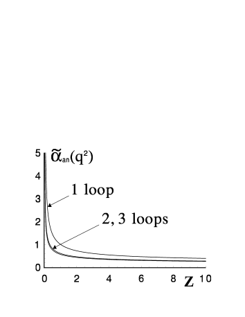
Figure 1: The QCD analytic invariant charge at different loop levels, $z=q^{2}/\Lambda^{2}$.

The developed model for the QCD analytic invariant charge possesses a number of appealing traits (see Refs. MPLA1,MPLA2). Namely, it has no unphysical singularities at any loop level; it contains no adjustable parameters; it incorporates ultraviolet asymptotic freedom with infrared (IR) enhancement in a single expression; it has universal behavior both in UV and IR regions at any loop level; it possesses a good higher loop and scheme stability. This model also enables one to describe various strong interaction processes both of perturbative and intrinsically nonperturbative nature (see papers IJMPA,QCD03,ConfV and references therein). It is of a primary importance to mention here that the analytic invariant charge (2) has recently been rediscovered when studying the conformal inversion symmetry related to the size distribution of instantons.[14] In particular, Eq. (2) was proved to reproduce explicitly this kind of symmetry. In turn, the latter is in a good agreement with the relevant lattice data by the UKQCD Collaboration[11] (see Refs. Schrempp and IJMPA for the details).

3 The Static Quark–Antiquark Potential

Let us proceed now to the construction of the static quark–antiquark potential. In the framework of the one-gluon exchange model it is related to the strong running coupling $\alpha(q^{2})$ by the 3-dimensional Fourier transformation

$$V(r)=-\frac{16\pi}{3}\int\limits_{0}^{\infty}\frac{\alpha(\bm{q}^{2})}{\bm{q}^{2}}\,\frac{\exp(i\bm{qr})}{(2\pi)^{3}}\,d{\bm{q}}.$$ (3)

Strictly speaking, this definition of the potential is justified for small distances ($r\lesssim 0.1\,$fm) only. For example, the lowest–lying bound states of heavy quarks can be described by employing the perturbative QCD.[15] However, at large distances ($r\gtrsim 0.5\,$fm), which play the crucial role in hadron spectroscopy, the perturbative approach blows up due to unphysical singularities (such as the Landau pole) of the strong running coupling. Nevertheless, the model (3), being complemented with a certain insight into the nonperturbative behavior of the QCD invariant charge, has proved to be successful for description both heavy–quark and light–quark systems (see, e.g., reviews Lucha91,Brambilla99,Kiselev1 and references therein for the details).

In this paper, for the construction of the static potential of the quark–antiquark interaction, we shall use the analytic invariant charge (2). After integration over angular variables, Eq. (3) in this case takes the form

$$V(r)=-\frac{32}{3\beta_{0}}\,\frac{1}{r_{0}}\int\limits_{0}^{\infty}\frac{p^{2}-1}{p^{2}\,\ln p^{2}}\,\frac{\sin(pR)}{pR}\,dp,$$ (4)

where $p=qr_{0}$, $R=r/r_{0}$, and $r_{0}$ is a reference scale of the dimension of length, which will be specified below. This integral diverges at the lower limit, that is a common feature of the models of such kind (see, e.g., Ref. Lucha91). We shall treat this divergence by employing the analytical regularization (see Eq. (10)).

The analysis of Eq. (4), performed in Ref. PRD1, elucidated only the leading asymptotic behavior of $V(r)$ at large distances. However, it is still desirable to examine at a more precise level the asymptotics of the quark–antiquark potential (4) in the both, ultraviolet and infrared regions. This objective can be achieved in the following way. First of all, let us introduce a dimensionless variable $Q=pR$ and rewrite Eq. (4):

$$V(r)=\frac{16}{3\beta_{0}}\,\frac{1}{r_{0}}\,\frac{1}{R}\int\limits_{0}^{\infty}\!\left(1-\frac{R^{2}}{Q^{2}}\right)\frac{\sin Q}{Q}\,\frac{dQ}{\ln R-\ln Q}.$$ (5)

Then, formally expanding the denominator of the integrand, one can find the asymptotic behavior of $V(r)$ at both small and large distances:

$$V(r) \simeq \frac{16}{3\beta_{0}}\,\frac{1}{r_{0}}\Biggl{[}\frac{1}{R}\sum_{n=0}^{n_{0}}\frac{1}{(\ln R)^{n+1}}\int\limits_{0}^{\infty}\frac{\sin Q}{Q}(\ln Q)^{n}\,dQ\nopagebreak$$ (6)

$$-R\sum_{m=0}^{m_{0}}\frac{1}{(\ln R)^{m+1}}\int\limits_{0}^{\infty}\frac{\sin Q}{Q^{3}}(\ln Q)^{m}\,dQ\Biggr{]}.$$

The values of $n_{0}$ and $m_{0}$ will be specified below.

For evaluation of the expansion coefficients in Eq. (6) it is worth considering an auxiliary integral of the form:

$$\int\limits_{0}^{\infty}Q^{t}\,\sin Q\,dQ=\sqrt{\pi}\,2^{t}\,\frac{\Gamma\left(1+\frac{t}{2}\right)}{\Gamma\left(\frac{1}{2}-\frac{t}{2}\right)}.$$ (7)

Differentiating this equation $n$ times with respect to variable $t$ we obtain

$$\int\limits_{0}^{\infty}Q^{t}\,(\ln Q)^{n}\,\sin Q\,dQ=v(n,t),$$ (8)

where

$$v(n,t)=\sqrt{\pi}\,\frac{d^{n}}{dt^{n}}\left[2^{t}\,\frac{\Gamma\left(1+\frac{t}{2}\right)}{\Gamma\left(\frac{1}{2}-\frac{t}{2}\right)}\right].$$ (9)

In Eq. (7) the parameter $t$ takes the values $0\leq|\mbox{Re}\,(t+1)|<1$ (see, e.g., Ref. RG). However, in order to determine the expansion coefficients of the second sum in Eq. (6), one has to go to the point $t=-3$, which is outside of this range. Nevertheless, it can be done by making use of the analytic continuation of the left-hand side of Eq. (7). This continuation is unique and it is defined obviously by the right-hand side of Eq. (7) all over the complex $t$–plane except for the points $t=-2N$, with $N$ being a natural number. Fortunately, we are not dealing with these values of the parameter $t$, and we can put

$$\int\limits_{0}^{\infty}\left.\frac{\sin Q}{Q^{s}}(\ln Q)^{n}\,dQ=v(n,t)\right|_{t=-s},\quad s\neq 2N\quad(N=1,2,3,...\,).$$ (10)

It should be noted here that this analytical continuation plays the role of regularization of the expansion coefficients in Eq. (6). It is also convenient to introduce the notations

$$u_{n}=\left.\frac{2}{\pi}\,v(n,t)\right|_{t=-1},\qquad\omega_{m}=-\left.\frac{2}{\pi}\,v(m,t)\right|_{t=-3}.$$ (11)

A few first coefficients (11) have a quite simple form, namely $u_{0}=1$,  $u_{1}=-\gamma$,  $u_{2}=\gamma^{2}+\pi^{2}/12$; and $\omega_{0}=1/2$,  $\omega_{1}=3/4-\gamma/2$,  $\omega_{2}=\gamma^{2}/2-3\gamma/2+\pi^{2}/24+7/4$, where $\gamma\simeq 0.57721...$ denotes the Euler’s constant (see Ref. IJMPA). It is worth noting here that the leading coefficients $u_{0}$, $\,\omega_{0}$, and $\omega_{1}$ have also been calculated in Ref. PRD1, but by making use of another technique.

Thus, the static quark–antiquark potential (6) can be represented now in the following form:

$$V(r)\simeq\frac{8\pi}{3\beta_{0}}\,\frac{1}{r_{0}}\left[\frac{1}{R}\sum_{n=0}^{n_{0}}\frac{u_{n}}{(\ln R)^{n+1}}+R\sum_{m=0}^{m_{0}}\frac{\omega_{m}}{(\ln R)^{m+1}}\right],\qquad R=\frac{r}{r_{0}}.$$ (12)

At small distances the potential (12) possesses the standard behavior, determined by the asymptotic freedom

$$V(r)=\frac{8\pi}{3\beta_{0}}\,\frac{1}{r_{0}}\,\frac{1}{R\,\ln R},\qquad r\to 0.$$ (13)

At the same time, it proves to be rising at large distances

$$V(r)=\frac{8\pi}{3\beta_{0}}\,\frac{1}{r_{0}}\,\frac{R}{2\,\ln R},\qquad r\to\infty,$$ (14)

implying the confinement of quarks. It is of a particular interest to mention here that a similar rising behavior of the $\mbox{Q}\overline{\mbox{Q}}$ potential has been proposed[21] a long time ago proceeding from the phenomenological assumptions.

Equation (12) describes the behavior of the static quark–antiquark potential (4) at small and large distances. However, its straightforward extrapolation to all distances encounters poles of different orders at the point $R=1$, which apparently is an artifact of the expansion (6). For the practical purposes it would be undoubtedly useful to derive an explicit expression for the $\mbox{Q}\overline{\mbox{Q}}$ potential applicable for $0<r<\infty$.

In order to construct an explicit interpolating formula for the quark–antiquark potential (4) we shall employ here the following method. Let us modify the expansion (12) in a “minimal” way, by adding terms which only subtract the singularities at the point $R=1$ and do not contribute to the derived asymptotics. This leads to the following expression for the static quark–antiquark potential

$$V(r) = \frac{8\pi}{3\beta_{0}}\,\frac{1}{r_{0}}\left\{\sum_{n=0}^{n_{0}}u_{n}\left[\frac{1}{R\,(\ln R)^{n+1}}\right]_{\mbox{\scriptsize Reg}}+\sum_{m=0}^{m_{0}}\omega_{m}\left[\frac{R}{(\ln R)^{m+1}}\right]_{\mbox{\scriptsize Reg}}\right\},$$ (15)

where $R=r/r_{0}$, and at the leading orders $[1/(R\,\ln R)]_{\mbox{\scriptsize Reg}}=1/(R\,\ln R)-1/P$, $[1/(R\,(\ln R)^{2})]_{\mbox{\scriptsize Reg}}=1/(R\,(\ln R)^{2})-1/P^{2}$, and $[R/\ln R]_{\mbox{\scriptsize Reg}}=R/\ln R-1/P$, $[R/(\ln R)^{2}]_{\mbox{\scriptsize Reg}}=R/(\ln R)^{2}-2/P-1/P^{2}$, $P=R-1$ (see also Ref. IJMPA).

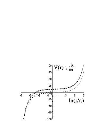
Figure 2: The quark–antiquark potential (15) in dimensionless units at different levels of approximation: $n_{0}=m_{0}=0$ (dashed curve), $n_{0}=m_{0}=4$ (solid curve), $n_{0}=m_{0}=5$ ($\blacktriangle$), and $n_{0}=m_{0}=10$ ($\blacksquare$). The one-loop perturbative result is shown by dotted curve.

The numerical analysis of Eq. (15) revealed that for practical purposes it is enough to retain the first five expansion terms ($n_{0}=m_{0}=4$) therein. It turns out that the potential (15) itself and the corresponding estimation of the value of parameter $\Lambda_{\mbox{\tiny QCD}}$ are not affected by higher–order contributions. In particular, the curves (15) for $n_{0}=m_{0}=5$ and for $n_{0}=m_{0}=10$ are practically indistinguishable of the curve corresponding to $n_{0}=m_{0}=4$ over the whole region $0<r<\infty$ (see Figure 2). And the higher–order estimations of the parameter $\Lambda_{\mbox{\tiny QCD}}$ vary within $0.5\,\%$ of the value obtained at the $n_{0}=m_{0}=4$ (see Sec. 4 further).

Thus, we arrive at the following explicit expression for the static quark–antiquark potential:

$$V(r) = V_{0}+\frac{8\pi}{3\beta_{0}}\,\frac{1}{r_{0}}\Biggl{\{}\frac{1}{R}\Biggl{[}\frac{1}{\ln R}-\frac{0.577}{(\ln R)^{2}}+\frac{1.156}{(\ln R)^{3}}-\frac{4.021}{(\ln R)^{4}}+\frac{15.018}{(\ln R)^{5}}\Biggr{]}$$ (16)

$$+R\Biggl{[}\frac{0.500}{\ln R}+\frac{0.461}{(\ln R)^{2}}+\frac{1.462}{(\ln R)^{3}}+\frac{3.185}{(\ln R)^{4}}+\frac{17.844}{(\ln R)^{5}}\Biggr{]}$$

$$+\frac{21.489}{1-R}-\frac{62.484}{(1-R)^{2}}+\frac{98.694}{(1-R)^{3}}-\frac{84.143}{(1-R)^{4}}+\frac{32.861}{(1-R)^{5}}\Biggr{\}},$$

where $R=r/r_{0}$. In order to reproduce the correct short-distance behavior of the $\mbox{Q}\overline{\mbox{Q}}$ potential, the dimensional parameter $r_{0}$ in this equation has to be identified with $\Lambda_{\overline{\mbox{\tiny MS}}}$ by the relation $r_{0}^{-1}=\Lambda\exp(\gamma)$ (see, e.g., Refs. Melles,Peter,Kiselev2). It is straightforward to verify that the potential (16) satisfies also the concavity condition

$$\frac{d\,V(r)}{d\,r}>0,\qquad\frac{d^{2}V(r)}{d\,r^{2}}\leq 0,$$ (17)

which is a general property of the gauge theories (see Ref. SB for the details).

4 Discussion

In this section we are going to apply the obtained results to the study of recent quenched lattice simulation data[10] on the static quark–antiquark potential. In particular, the value of the parameter $\Lambda_{\mbox{\tiny QCD}}$ will be estimated by comparing the derived expression for the $\mbox{Q}\overline{\mbox{Q}}$ potential (16) with these lattice data.

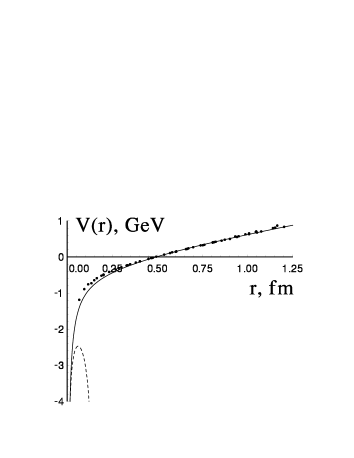
Figure 3: Comparison of the quark–antiquark potential $V(r)$ defined by Eq. (16) (solid curve) with the quenched lattice simulation data[10] ($\bullet$). The values of the parameters are: $\Lambda=670\,$MeV, $n_{\mbox{\tiny f}}=0$, $V_{0}=-3.164\,$GeV. The dashed curve corresponds to the relevant one-loop perturbative result.

Thus, a fit of the quark–antiquark potential (16) to the quenched lattice simulation data[10] has been performed with the use of the least square method. The varied parameters in Eq. (16) were $r_{0}$ and the additive self–energy constant $V_{0}$. The result of the fit is presented in Figure 3. This figure shows that in the nonperturbative physically–relevant range $0.3\,\mbox{fm}\lesssim r\lesssim 1.2\,\mbox{fm}$, in which the average quark separations $\sqrt{\langle r^{2}\rangle}$ for quarkonia sits,[26] the $\mbox{Q}\overline{\mbox{Q}}$ potential (16) reproduces the lattice data[10] fairly well. At the same time, in the region $r\lesssim 0.05\,\mbox{fm}$ the derived potential coincides with the perturbative result (dashed curve in Fig. 3). The difference between the lattice data and the expression (16) in the intermediate range $0.05\,\mbox{fm}\lesssim r\lesssim 0.3\,\mbox{fm}$ may be explained by the presence of additional nonperturbative contributions at these distances (see, e.g., Refs. ShortString,Lee). But the detailed investigation of this matter is beyond the scope of the paper.

Thus, the estimation of the parameter $\Lambda_{\mbox{\tiny QCD}}$ in the course of this comparison gives $\Lambda^{\!(n_{\mbox{\tiny f}}=0)}=(670\pm 8)\,$MeV (this value corresponds to the one-loop level with $n_{\mbox{\scriptsize f}}=0$ active quarks). The uncertainty here has been calculated by making use of the “$3\sigma$–criterion” (see Ref. Data). It is worth noting that the fit with the use of the maximum likelihood method results in even better reproduction of the lattice data and gives a similar value $\Lambda^{\!(n_{\mbox{\tiny f}}=0)}\simeq 645\,$MeV. Further, in order to collate the obtained estimation with the earlier ones, one has to continue it to the region of three active quarks. It was performed by employing the matching procedure, and gives the value $\Lambda^{\!(n_{\mbox{\tiny f}}=3)}=(590\pm 10)\,$MeV. The latter is in a good agreement with all the previous estimations of this parameter[6, 13] [$\Lambda^{\!(n_{\mbox{\tiny f}}=3)}=(550\pm 50)\,$MeV] in the framework of the approach in hand.

5 Conclusion

In the paper the QCD analytic invariant charge has been applied to study of the quenched lattice simulation data on the static quark–antiquark potential. This strong running coupling enables one to obtain explicitly the confining quark–antiquark potential in the framework of the one-gluon exchange model. A technique for evaluation the integrals of a specific form, developed in this paper, allows one to examine the asymptotic behavior of the derived potential at small and large distances with high accuracy. An explicit formula for the quark–antiquark potential, which interpolates between these asymptotics and satisfies the concavity condition, is obtained. The derived potential has the standard form determined by asymptotic freedom at small distances. At the same time, in the nonperturbative physically–relevant region $0.3\,\mbox{fm}\lesssim r\lesssim 1.2\,\mbox{fm}$ this potential agrees fairly well with the lattice simulation data. The value of the parameter $\Lambda_{\mbox{\tiny QCD}}$ is estimated for the case of pure gluodynamics. It is found to be consistent with all the previous estimations of $\Lambda_{\mbox{\tiny QCD}}$ in the framework of the approach developed.

References

- [1] P.J. Redmond, Phys. Rev. 112, 1404 (1958); P.J. Redmond and J.L. Uretsky, Phys. Rev. Lett. 1, 147 (1958).
- [2] N.N. Bogoliubov, A.A. Logunov, and D.V. Shirkov, Zh. Exp. Teor. Fiz. 37, 805 (1959) [Sov. Phys. JETP 37, 574 (1960)].
- [3] D.V. Shirkov and I.L. Solovtsov, Phys. Rev. Lett. 79, 1209 (1997).
- [4] I.L. Solovtsov and D.V. Shirkov, Teor. Mat. Fiz. 120, 482 (1999) [Theor. Math. Phys. 120, 1220 (1999)]; D.V. Shirkov, Eur. Phys. J. C22, 331 (2001).
- [5] A.V. Nesterenko, Phys. Rev. D62, 094028 (2000).
- [6] A.V. Nesterenko, Phys. Rev. D64, 116009 (2001).
- [7] A.V. Nesterenko, Int. J. Mod. Phys. A18, 5475 (2003).
- [8] A.V. Nesterenko, Mod. Phys. Lett. A15, 2401 (2000).
- [9] A.V. Nesterenko and I.L. Solovtsov, Mod. Phys. Lett. A16, 2517 (2001).
- [10] G.S. Bali et al., (SESAM and TL Collaborations), Phys. Rev. D62, 054503 (2000).
- [11] D.A. Smith and M.J. Teper (UKQCD Collaboration), Phys. Rev. D58, 014505 (1998); A. Ringwald and F. Schrempp, Phys. Lett. B459, 249 (1999); B503, 331 (2001).
- [12] A.V. Nesterenko, in Proceedings of the Tenth High Energy Physics International Conference in Quantum Chromodynamics, Montpellier, France, 2003 (to be published); arXiv: hep-ph/0307283.
- [13] A.V. Nesterenko, in Proceedings of the Fifth International Conference on Quark Confinement and the Hadron Spectrum, Gargnano, Italy, 2002, edited by N. Brambilla and G. Prosperi (World Scientific, Singapore, 2003), p. 288; arXiv: hep-ph/0210122.
- [14] F. Schrempp, J. Phys. G28, 915 (2002).
- [15] S. Titard and F.J. Yndurain, Phys. Rev. D49, 6007 (1994).
- [16] W. Lucha, F.F. Schoberl, and D. Gromes, Phys. Rep. 200, 127 (1991).
- [17] N. Brambilla and A. Vairo, arXiv: hep-ph/9904330.
- [18] V.V. Kiselev and A.K. Likhoded, Usp. Fiz. Nauk 172, 497 (2002) [Sov. Phys. Usp. 45, 455 (2002)].
- [19] R. Levine and Y. Tomozawa, Phys. Rev. D19, 1572 (1979).
- [20] I.S. Gradshteyn and I.M. Ryzhik, Table of Integrals, Series, and Products, edited by A. Jeffrey (Academic, London, 1994).
- [21] G. Fogleman, D.B. Lichtenberg, and J.G. Wills, Lett. Nuovo Cimento 26, 369 (1979); D.B. Lichtenberg and J.G. Wills, Nuovo Cimento A47, 483 (1978).
- [22] M. Melles, Phys. Rev. D62, 074019 (2000).
- [23] M. Peter, Phys. Rev. Lett. 78, 602 (1997); Nucl. Phys. B501, 471 (1997).
- [24] V.V. Kiselev, A.E. Kovalsky, and A.I. Onishchenko, Phys. Rev. D64, 054009 (2001); V.V. Kiselev, A.K. Likhoded, O.N. Pakhomova, and V.A. Saleev, ibid. D66, 034030 (2002).
- [25] E. Seiler, Phys. Rev. D18, 482 (1978); C. Bachas, ibid. D33, 2723 (1986).
- [26] G.S. Bali, K. Schilling, and A. Wachter, Phys. Rev. D56, 2566 (1997); G.S. Bali and P. Boyle, ibid. D59, 114504 (1999).
- [27] W. Buchmuller, G. Grunberg, and S.-H. H. Tye, Phys. Rev. Lett. 45, 103 (1980); 45, 587(E) (1980); W. Buchmuller and S.-H. H. Tye, Phys. Rev. D24, 132 (1981).
- [28] K. Hagiwara, A.D. Martin, and A.W. Peacock, Z. Phys. C33, 135 (1986).
- [29] R. Akhoury and V.I. Zakharov, Phys. Lett. B438, 165 (1998); G.S. Bali, ibid. B460, 170 (1999).
- [30] T. Lee, Phys. Rev. D67, 014020 (2003).
- [31] S.L. Meyer, Data Analysis for Scientists and Engineers (Wiley, New York, 1975).
- [32] W. Celmaster and F.S. Henyey, Phys. Rev. D18, 1688 (1978).