Associated Higgs production with top quarks
at the Large Hadron Collider: NLO QCD corrections

Abstract

We present in detail the calculation of the ${\cal O}(\alpha_{s}^{3})$ inclusive total cross section for the process $pp\to t\bar{t}h$, in the Standard Model, at the CERN Large Hadron Collider with center-of-mass energy $\sqrt{s_{\scriptscriptstyle H}}\!=\!14$ TeV. The calculation is based on the complete set of virtual and real ${\cal O}(\alpha_{s})$ corrections to the parton level processes $q\bar{q}\to t\bar{t}h$ and $gg\to t\bar{t}h$, as well as the tree level processes $(q,\bar{q})g\to t\bar{t}h+(q,\bar{q})$. The virtual corrections involve the computation of pentagon diagrams with several internal and external massive particles, first encountered in this process. The real corrections are computed using both the single and the two cutoff phase space slicing method. The next-to-leading order QCD corrections significantly reduce the renormalization and factorization scale dependence of the Born cross section and moderately increase the Born cross section for values of the renormalization and factorization scales above $m_{t}$.

I Introduction

One of the critical goals of present and future colliders is the study of the electroweak symmetry breaking mechanism and the origin of fermion masses. If the introduction of one or more Higgs fields is responsible for the breaking of the electroweak symmetry and for the generation of fermion masses, then one Higgs boson should be relatively light. The present lower bounds on the Higgs boson mass from direct searches at LEP2 are $M_{h}\!>\!114.4$ GeV (at $95\%$ CL) Note/2002-03 (July 2002) for the Standard Model (SM) Higgs boson ($h$), and $M_{h^{0}}\!>\!91.0$ GeV and $M_{A^{0}}\!>\!91.9$ GeV (at $95\%$ CL, $0.5\!<\!\tan\beta\!<\!2.4$ excluded) Note/2001-04 (July 2001) for the light scalar ($h^{0}$) and pseudoscalar ($A^{0}$) Higgs bosons of the minimal supersymmetric standard model (MSSM). At the same time, global SM fits to electroweak precision data imply $M_{h}<211$ GeV (at $95\%$ CL) LEPEWWG/2003-01 (April 2003), while the MSSM requires the existence of a scalar Higgs boson lighter than about 130 GeV. The possibility of a Higgs boson discovery in the mass range near 115-130 GeV thus seems increasingly likely.

The associated production of a Higgs boson with a $t\bar{t}$ pair can play a very important role at hadron colliders as has been suggested by many studies over the past several years Marciano and Paige (1991); Collaboration (1994, 1999); Goldstein et al. (2001). In particular, it is an important discovery channel for a SM-like Higgs boson at the LHC if $M_{h}\!<\!130$ GeV Collaboration (1999); Richter-Was and Sapinski (1999); Beneke et al. (2000); Drollinger et al. (2001). Although the event rate is small, the signature is quite distinctive. Given the statistics expected at the LHC, $pp\to t\bar{t}h$, with $h\to b\bar{b},\tau^{+}\tau^{-},W^{+}W^{-},\gamma\gamma$ will also be instrumental to the determination of the couplings of a discovered Higgs boson, and will in particular give the only handle on a direct measurement of the top quark Yukawa coupling Beneke et al. (2000); Zeppenfeld et al. (2000); Zeppenfeld (2002); Belyaev and Reina (2002); Maltoni et al. (2002).

The total cross section for $pp\to t\bar{t}h$ has been known at tree-level, i.e. at leading order (LO) of QCD, for quite some time Kunszt (1984); Ng and Zakarauskas (1984). Next-to-leading order (NLO) QCD corrections are crucial in order to reduce the dependence of the cross section on the renormalization and factorization scales. The calculation of the total cross section for $pp\to t\bar{t}h$ to ${\cal O}(\alpha_{s}^{3})$ has been performed by the Authors of Refs. Beenakker et al. (2001, 2003) and by our group. The results of the two independent calculations have been compared and they are in very good agreement. In Ref. Dawson et al. (2003), we presented our first numerical results for the total inclusive NLO QCD cross section for $pp\to t\bar{t}h$ at the LHC center of mass energy, $\sqrt{s_{\scriptscriptstyle H}}\!=\!14$ TeV. Here we provide a detailed description of the calculation.

At the LHC center-of-mass energy, the dominant subprocess for $t\bar{t}h$ production is $gg\to t\bar{t}h$, but the other subprocesses, $q\bar{q}\to t\bar{t}h$ and $(q,\bar{q})g\to t\bar{t}h+(q,\bar{q})$, which contribute to the cross section at ${\cal O}(\alpha_{s}^{3})$, cannot be neglected and are included in this calculation. The NLO QCD corrections to the $q\bar{q}\to t\bar{t}h$ subprocess constitute a gauge invariant subset of the entire NLO QCD calculation and have been presented in Refs. Reina and Dawson (2001); Reina et al. (2002) to which we refer for a thorough discussion of the results. Here we concentrate on a detailed description of the calculation of the ${\cal O}(\alpha_{s})$ corrections to the $gg\to t\bar{t}h$ subprocess. The Feynman diagrams contributing to $gg\to t\bar{t}h$ at lowest order are shown in Fig. 1, while the ${\cal O}(\alpha_{s})$ virtual and real corrections are given in Figs. 2-5 and Fig. 6, respectively.

The main challenge in the calculation of the ${\cal O}(\alpha_{s})$ virtual corrections comes from the presence of pentagon diagrams with several massive external and internal particles. The pentagon scalar and tensor Feynman integrals originating from these diagrams present either analytical (scalar) or numerical (tensor) challenges. We have calculated the pentagon scalar integrals as linear combinations of scalar box integrals using the method of Ref. Bern et al. (1993, 1994), and cross checked them using the techniques of Ref. Denner (1993). Pentagon tensor integrals have been calculated and cross checked in two ways: numerically, by isolating the numerical instabilities and extrapolating from the numerically safe to the numerically unsafe region using various methods; and analytically, by reducing them to a numerically stable form. The real corrections have been computed using the phase space slicing method, in both the double (for a review see, e.g. Harris and Owens (2002)) and single Giele and Glover (1992); Giele et al. (1993); Keller and Laenen (1999) cutoff approaches. Together with the corresponding $q\bar{q}\to t\bar{t}h$ calculation Reina and Dawson (2001); Reina et al. (2002), this is the first application of the single cutoff phase space slicing method to a cross section involving more than one massive particle in the final state and agreement between the two cutoff and the single cutoff approaches is a strong check of the calculation.

The outline of our paper is as follows. In Section II we summarize the general structure of the NLO cross section for $pp\to t\bar{t}h$. In Section III we briefly review the case of the LO cross section for $pp\to t\bar{t}h$, introducing some fundamental notation. We proceed in Sections IV and V to present the details of the calculation of both the virtual and real parts of the NLO QCD corrections to $gg\to t\bar{t}h$. Section V also includes a discussion of the tree level $(q,\bar{q})g\to t\bar{t}h+(q,\bar{q})$ processes. In Section VI we explicitly show the factorization of the initial state infrared singularities into the gluon distribution functions, and finally summarize our results for the NLO inclusive total cross section for $pp\to t\bar{t}h$ at the LHC in Eqs. (83) and (1))-(2)). Finally, numerical results for the total cross section are presented in Section VII. We collect most of the technical details, including a list of box and pentagon integrals, in a series of Appendices.

II The calculation: general setup

The inclusive total cross section for $pp\to t\bar{t}h$ at ${\cal O}(\alpha_{s}^{3})$ can be written as:

$$\sigma_{\scriptscriptstyle NLO}(pp\to t\bar{t}h)=$$

$$\sum_{ij}\frac{1}{1+\delta_{ij}}\int dx_{1}dx_{2}\left[{\cal F}_{i}^{p}(x_{1},\mu){\cal F}_{j}^{p}(x_{2},\mu){\hat{\sigma}}^{ij}_{\scriptscriptstyle NLO}(x_{1},x_{2},\mu)+(1\leftrightarrow 2)\right]\,\,\,,$$ (1)

where ${\cal F}_{i}^{p}$ are the NLO parton distribution functions (PDFs) for parton $i$ in a proton, defined at a generic factorization scale $\mu_{f}\!=\!\mu$, and ${\hat{\sigma}}^{ij}_{\scriptscriptstyle NLO}$ is the ${\cal O}(\alpha_{s}^{3})$ parton-level total cross section for incoming partons $i$ and $j$, made of the channels $q\bar{q},gg\to t\bar{t}h$ and $(q,\bar{q})g\to t\bar{t}h(q,\bar{q})$, and renormalized at an arbitrary scale $\mu_{r}$ which we also take to be $\mu_{r}\!=\!\mu$. Throughout this paper we will always assume the factorization and renormalization scales to be equal, $\mu_{r}\!=\!\mu_{f}\!=\!\mu$, unless differently specified. The partonic center-of-mass energy squared, $s$, is given in terms of the hadronic center-of-mass energy squared, $s_{\scriptscriptstyle H}$, by $s=x_{1}x_{2}s_{\scriptscriptstyle H}$. At the LHC center-of-mass energy the cross section is dominated by the $gg$ initial state, although the other contributions cannot be neglected and are included in this calculation.

We write the NLO parton-level total cross section ${\hat{\sigma}}_{\scriptscriptstyle NLO}^{ij}(x_{1},x_{2},\mu)$ as:

$${\hat{\sigma}}_{\scriptscriptstyle NLO}^{ij}(x_{1},x_{2},\mu) = \alpha_{s}^{2}(\mu)\left\{f_{\scriptscriptstyle LO}^{ij}(x_{1},x_{2})+\frac{\alpha_{s}(\mu)}{4\pi}f_{\scriptscriptstyle NLO}^{ij}(x_{1},x_{2},\mu)\right\}$$ (2)

$$\equiv {\hat{\sigma}}_{\scriptscriptstyle LO}^{ij}(x_{1},x_{2},\mu)+\delta{\hat{\sigma}}_{\scriptscriptstyle NLO}^{ij}(x_{1},x_{2},\mu)\,\,\,,$$

where $\alpha_{s}(\mu)$ is the strong coupling constant renormalized at the arbitrary scale $\mu_{r}\!=\!\mu$, ${\hat{\sigma}}_{\scriptscriptstyle LO}^{ij}(x_{1},x_{2},\mu)$ is the ${\cal O}(\alpha_{s}^{2})$ Born cross section, and $\delta{\hat{\sigma}}_{\scriptscriptstyle NLO}^{ij}(x_{1},x_{2},\mu)$ consists of the ${\cal O}(\alpha_{s})$ corrections to the Born cross sections for $gg,q\bar{q}\to t\bar{t}h$ and of the tree level $(q,\bar{q})g\to t\bar{t}h(q,\bar{q})$ processes, including the effects of mass factorization (see Section VI). $\delta{\hat{\sigma}}_{\scriptscriptstyle NLO}^{ij}(x_{1},x_{2},\mu)$ can be written as the sum of two terms:

$$\delta{\hat{\sigma}}_{\scriptscriptstyle NLO}^{ij}(x_{1},x_{2},\mu) = \int d(PS_{3})\overline{\sum}|{\cal A}_{virt}(ij\to t\bar{t}h)|^{2}+\int d(PS_{4})\overline{\sum}|{\cal A}_{real}(ij\to t\bar{t}h+l)|^{2}$$ (3)

$$\equiv \hat{\sigma}^{ij}_{virt}(x_{1},x_{2},\mu)+\hat{\sigma}^{ij}_{real}(x_{1},x_{2},\mu)\,\,\,,$$

where $|{\cal A}_{virt}(ij\to t\bar{t}h)|^{2}$ and $|{\cal A}_{real}(ij\to t\bar{t}h+l)|^{2}$ (for $ij\!=\!q\bar{q},gg$ and $l\!=\!g$, or $ij\!=\!qg,\bar{q}g$ and $l\!=\!q,\bar{q}$) are respectively the ${\cal O}(\alpha_{s}^{3})$ terms of the squared matrix elements for the $ij\rightarrow t\bar{t}h$ and $ij\rightarrow t\bar{t}h+l$ processes, and $\overline{\sum}$ indicates that they have been averaged over the initial state degrees of freedom and summed over the final state ones. Moreover, $d(PS_{3})$ and $d(PS_{4})$ in Eq. (3) denote the integration over the corresponding three and four-particle phase spaces respectively. The first term in Eq. (3) represents the contribution of the virtual one gluon corrections to $q\bar{q}\to t\bar{t}h$ and $gg\to t\bar{t}h$, while the second one is due to the real one gluon and real one quark/antiquark emission, i.e. $q\bar{q},gg\to t\bar{t}h+g$ and $qg(\bar{q}g)\to t\bar{t}h+q(\bar{q})$.

The ${\cal O}(\alpha_{s})$ virtual and real corrections to $q\bar{q}\to t\bar{t}h$ have been discussed in detail in Ref. Reina et al. (2002), and will not be repeated here. In the following sections we present the general structure of the ${\cal O}(\alpha_{s})$ virtual and real corrections to $gg\to t\bar{t}h$. The contribution of the $(q,\bar{q})g$ initiated process will be considered in Section V, when dealing with the real part of the ${\cal O}(\alpha_{s}^{3})$ cross section. The results presented in the following sections have been obtained by two completely independent calculations, based on a combination of FORM Vermaseren (2000) and Maple codes in one case, and on the Mathematica based code Tracer Jamin and Lautenbacher (1993) in the other. The matrix elements squared for the tree level processes $gg\to t\bar{t}h$, $gg\to t\bar{t}h+g$, and $(q,\bar{q})g\to t\bar{t}h+(q,\bar{q})$ have been checked with Madgraph Stelzer and Long (1994). The numerical results presented in Section VII have been obtained with two independent Fortran codes.

Finally, we observe that the scale dependence of the total cross section at NLO is dictated by renormalization group arguments, and $f_{\scriptscriptstyle NLO}^{ij}(x_{1},x_{2},\mu)$ in Eq. (2) must be of the form:

$$f_{\scriptscriptstyle NLO}^{ij}(x_{1},x_{2},\mu)=f_{1}^{ij}(x_{1},x_{2})+\tilde{f}_{1}^{ij}(x_{1},x_{2})\ln\left(\frac{\mu^{2}}{s}\right)\,\,\,,$$ (4)

with $\tilde{f}_{1}^{ij}(x_{1},x_{2})$ given by:

$$\tilde{f}_{1}^{ij}(x_{1},x_{2}) = 2\,\left\{4\pi b_{0}f^{ij}_{\scriptscriptstyle LO}(x_{1},x_{2})-\sum_{k}\left[\int_{\rho}^{1}dz_{1}P_{ik}(z_{1})f^{kj}_{\scriptscriptstyle LO}(x_{1}z_{1},x_{2})\right.\right.$$ (5)

$$+ \left.\left.\int_{\rho}^{1}dz_{2}P_{jk}(z_{2})f^{ik}_{\scriptscriptstyle LO}(x_{1},x_{2}z_{2})\right]\right\}\,\,\,,$$

where $\rho\!=\!(2m_{t}+M_{h})^{2}/s$, $P_{ij}(z)$ denotes the lowest-order regulated Altarelli-Parisi splitting function Altarelli and Parisi (1977) of parton $i$ into parton $j$, when $j$ carries a fraction $z$ of the momentum of parton $i$, (see e.g. Section V), and $b_{0}$ is determined by the one-loop renormalization group evolution of the strong coupling constant $\alpha_{s}$:

$$\frac{d\alpha_{s}(\mu)}{d\ln(\mu^{2})}=-b_{0}\alpha_{s}^{2}+{\cal O}(\alpha_{s}^{3})\,\,\,\,\,,\,\,\,\,\,b_{0}=\frac{1}{4\pi}\left(\frac{11}{3}N-\frac{2}{3}n_{lf}\right)\,\,\,,$$ (6)

with $N=3$, the number of colors, and $n_{lf}\!=\!5$, the number of light flavors. The origin of the terms in Eq. (5) will become manifest in Sections IV, V, and VI when we describe in detail the calculation of both virtual and real ${\cal O}(\alpha_{s})$ corrections.

III The tree level cross section for $gg\to t\bar{t}h$

The tree level amplitude for the process

$$g^{A}(q_{1})+g^{B}(q_{2})\to t(p_{t})+\bar{t}(p_{t}^{\prime})+h(p_{h})\;,$$

where $q_{1}+q_{2}=p_{t}+p_{t}^{\prime}+p_{h}$ and $A,B$ denote the color of the incoming gluons, is obtained from the three classes of Feynman diagrams represented in Fig. 1, identified as $s-$channel, $t-$channel, and $u-$channel diagrams respectively. We find it convenient to organize the color structure of both the tree level amplitude and the one-loop virtual amplitude in terms of only two color factors, one symmetric and one antisymmetric in the color indices of the initial gluons. Following this prescription, the tree level amplitude for $gg\to t\bar{t}h$ can be written as:

$${\cal A}_{0}={\cal A}_{0}^{nab}[T^{A},T^{B}]+{\cal A}_{0}^{ab}\{T^{A},T^{B}\}\,\,\,,$$ (7)

where $T^{A,B}=\lambda^{A,B}/2$ in terms of the Gell-Mann matrices $\lambda^{A,B}~{}$. ${\cal A}_{0}^{ab}$ and ${\cal A}_{0}^{nab}$ correspond to the terms in the amplitude that are proportional respectively to the abelian (or symmetric) and non-abelian (or antisymmetric) color factors and are explicitly given by:

$${\cal A}_{0}^{ab}=\frac{1}{2}({\cal A}_{0,t}+{\cal A}_{0,u})\,\,\,,\,\,\,{\cal A}_{0}^{nab}={\cal A}_{0,s}+\frac{1}{2}({\cal A}_{0,t}-{\cal A}_{0,u})\,\,\,,$$ (8)

where ${\cal A}_{0,s}$, ${\cal A}_{0,t}$, and ${\cal A}_{0,u}$ are the amplitudes corresponding to the sum of the $s-$channel, $t-$channel, and $u-$channel tree level diagrams in Fig. 1. ${\cal A}_{0,s}$, ${\cal A}_{0,t}$, and ${\cal A}_{0,u}$ are given explicitly in Appendix A.

Due to the orthogonality between symmetric and antisymmetric color factors, the tree level amplitude squared takes the very simple form:

$$\overline{\sum}|{\cal A}_{0}|^{2}=\overline{\sum}\left[\frac{N}{2}(N^{2}-1)\left(|{\cal A}_{0}^{nab}|^{2}+|{\cal A}_{0}^{ab}|^{2}\right)-\frac{1}{N}(N^{2}-1)|{\cal A}_{0}^{ab}|^{2}\right]\,\,\,,$$ (9)

from which we can derive the LO partonic cross section, upon integration over the final state phase space:

$${\hat{\sigma}}_{\scriptscriptstyle LO}^{ij}(x_{1},x_{2},\mu)=\int d(PS_{3})\overline{\sum}|{\cal A}_{0}|^{2}(x_{1},x_{2},\mu)\,\,\,,$$ (10)

where the dependence of $|{\cal A}_{0}|^{2}$ on $x_{1}$ and $x_{2}$ (through $s\!=\!x_{1}x_{2}s_{H}$) and on the renormalization scale $\mu$ (through $\alpha_{s}(\mu))$) has been made explicit.

When averaging over the polarization states of the initial gluons, the polarization sum of the gluon polarization vectors, $\epsilon_{\mu}(q_{1},\lambda_{1})$ and $\epsilon_{\nu}(q_{2},\lambda_{2})$, has to be performed in such a way that only the physical (transverse) polarization states of the gluons contribute to the matrix element squared. We adopt the general prescription:

$$\sum_{\lambda_{i}=1,2}\epsilon_{\mu}(q_{i},\lambda_{i})\epsilon_{\nu}^{*}(q_{i},\lambda_{i})=-g_{\mu\nu}+\frac{n_{i\mu}q_{i\nu}+q_{i\mu}n_{i\nu}}{n_{i}\cdot q_{i}}-\frac{n_{i}^{2}q_{i\mu}q_{j\nu}}{(n_{i}\cdot q_{i})^{2}}\,\,\,,$$ (11)

where $i\!=\!1,2$ and the arbitrary vectors $n_{i}$ have to satisfy the relations:

$$n_{i}^{\mu}\sum_{\lambda_{i}=1,2}\epsilon_{\mu}(q_{i},\lambda_{i})\epsilon_{\nu}^{*}(q_{i},\lambda_{i})=0\,\,\,\,,\,\,\,\,n_{i}^{\nu}\sum_{\lambda_{i}=1,2}\epsilon_{\mu}(q_{i},\lambda_{i})\epsilon_{\nu}^{*}(q_{i},\lambda_{i})=0\,\,\,,$$ (12)

together with $n_{i}^{2}\!\neq\!0$ and $n_{1}\!\neq\!n_{2}$ We choose $n_{1}\!=\!q_{2}$ and $n_{2}\!=\!q_{1}$, such that:

$$\sum_{\lambda_{i}=1,2}\epsilon_{\mu}(q_{i},\lambda_{i})\epsilon_{\nu}^{*}(q_{i},\lambda_{i})=-g_{\mu\nu}+2\frac{q_{1\mu}q_{2\nu}+q_{2\mu}q_{1\nu}}{s}\,\,\,.$$ (13)

Finally, the entire calculation is performed using Feynman gauge for both internal and external gluons.

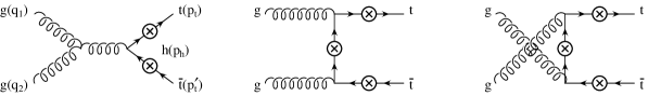
Figure 1: Feynman diagrams contributing to the tree level process $gg\to t\bar{t}h$. The circled crosses indicate all possible insertions of the final state Higgs boson leg, each insertion corresponding to a different diagram.

IV NLO virtual QCD corrections to $gg\to t\bar{t}h$: the $\hat{\sigma}_{virt}^{gg}$ cross section.

The ${\cal O}(\alpha_{s})$ virtual corrections to the $gg\to t\bar{t}h$ tree level process consist of the self-energy, vertex, box, and pentagon diagrams illustrated in Figs. 2-5. The ${\cal O}(\alpha_{s}^{3})$ contribution to the virtual amplitude squared of Eq. (3) can then be written as:

$$\overline{\sum}|{\cal A}_{virt}(gg\to t\bar{t}h)|^{2}=\sum_{D_{i,j}}\overline{\sum}\left({\cal A}_{0}{\cal A}_{D_{i,j}}^{*}+{\cal A}_{0}^{*}{\cal A}_{D_{i,j}}\right)=\sum_{D_{i,j}}\overline{\sum}2\,{\cal R}e\left({\cal A}_{0}{\cal A}_{D_{i,j}}^{*}\right)\,\,\,,$$ (14)

where ${\cal A}_{0}$ is the tree level amplitude given in Eq. (7), while ${\cal A}_{D_{i,j}}$ denotes the amplitude for a class of virtual diagrams that only differ by the insertion of the final state Higgs boson leg, i.e. $D_{i,j}=\sum_{k}D_{i,j}^{(k)}$ with $D_{i}\!=\!S_{i},V_{i},B_{i},P_{i}$, $j=s,t,u$, and $k$ running over all possible Higgs boson insertions, as illustrated in Figs. 2-5.

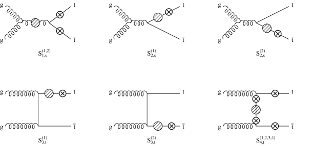
Figure 2: ${\cal O}(\alpha_{s})$ virtual corrections to $gg\to t\bar{t}h$: self-energy diagrams. The shaded blobs denote standard one-loop QCD corrections to the gluon and top quark propagators respectively. The circled crosses denote all possible insertions of the final state Higgs boson leg, each insertion corresponding to a different diagram. All $t$-channel diagrams (labeled as $S_{i,t}^{(j)}$) have corresponding $u$-channel diagrams.

Figure 3: ${\cal O}(\alpha_{s})$ virtual corrections to $gg\to t\bar{t}h$: vertex diagrams. The shaded blobs denote standard one-loop QCD corrections to the $ggg$, $gt\bar{t}$, or $ht\bar{t}$ vertices respectively. The circled crosses denote all possible insertions of the final Higgs boson leg, each insertion corresponding to a different diagram. Diagrams with a closed fermion loop have to be counted twice, once for each orientation of the loop fermion line. All $t$-channel diagrams (labeled as $V_{i,t}^{(j)}$) have corresponding $u$-channel diagrams.

Figure 4: ${\cal O}(\alpha_{s})$ virtual corrections to $gg\to t\bar{t}h$: box diagrams. The circled crosses denote all possible insertions of the final Higgs boson leg, each insertion corresponding to a different diagram. Diagrams with a closed fermion loop have to be counted twice, once for each orientation of the loop fermion line. All $t$-channel diagrams (labeled as $B_{i,t}^{(j)}$) have corresponding $u$-channel diagrams.

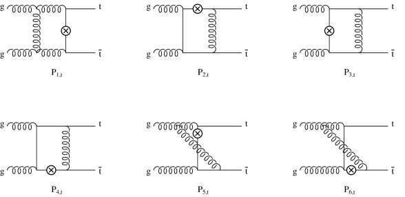
Figure 5: ${\cal O}(\alpha_{s})$ virtual corrections to $gg\to t\bar{t}h$: pentagon diagrams. The circled crosses denote all possible insertions of the final Higgs boson leg, each insertion corresponding to a different diagram. All $t$-channel diagrams (labeled as $P_{i,t}$) have corresponding $u$-channel diagrams.

The amplitude of each virtual diagram (${\cal A}_{D_{i,j}}$) is calculated as a linear combination of fundamental Dirac structures with coefficients that depend on both tensor and scalar one-loop Feynman integrals with up to five denominators. The tensor integrals are further reduced in terms of scalar one-loop integrals using standard techniques ’t Hooft and Veltman (1979); Passarino and Veltman (1979). The ${\cal O}(\alpha_{s})$ virtual corrections to $gg\to t\bar{t}h$ involve pentagon tensor integrals of rank higher than one, i.e. Feynman integrals with five denominators and more than one Lorentz tensor index. These pentagon tensor integrals are not present in the corresponding corrections for $q\bar{q}\to t\bar{t}h$. This introduces a new difficulty in the calculation, due to the numerical instabilities that may arise as a consequence of the proportionality of the tensor integral coefficients to higher powers of the inverse Gram determinant (GD) of the full $gg\to t\bar{t}h$ phase space. Indeed, the standard techniques introduced in Refs. ’t Hooft and Veltman (1979); Passarino and Veltman (1979) allow us to rewrite a tensor integral as a linear combination of the linearly independent tensor structures that can be built, for a given tensor rank, out of the independent external momenta and the metric tensor. The coefficients of the linearly independent tensor structures can be found by solving a system of linear equations, one for each independent tensor structure. As a result, they are proportional to inverse powers of the so called Gram determinant (GD), of the form ${\rm GD}\!=\!\mbox{det}(p_{i}\!\cdot\!p_{j})$ with $p_{i}$ and $p_{j}$ generic independent external momenta (for $i,j\!=\!1,\dots,4$, since only four out of the five external momenta are independent). The higher the rank of the original tensor integral, the higher the inverse power of GD that appears in the coefficients of its tensor decomposition.

To briefly illustrate the problem, we parameterize the Gram determinant in terms of the $t\bar{t}h$ phase space variables as

$${\rm GD} = -\frac{[s-(2m_{t}+M_{h})^{2}]}{64}[M_{h}^{4}+(s-\bar{s}_{t\bar{t}})^{2}-2M_{h}^{2}(s+\bar{s}_{t\bar{t}})]\,s\,\bar{s}_{t\bar{t}}\sin^{2}\theta_{t\bar{t}}\sin^{2}\phi_{t\bar{t}}\sin^{2}\theta\,\,\,,$$

where $s\!=\!x_{1}x_{2}s_{\scriptscriptstyle H}$ is the partonic center-of-mass energy squared, and the $t\bar{t}h$ phase space has been expressed in terms of a time-like invariant $\bar{s}_{t\bar{t}}\!=\!(p_{t}+p_{t}^{\prime})^{2}$, polar angles ($\theta,\theta_{t\bar{t}}$) and azimuthal angles ($\phi,\phi_{t\bar{t}}$) in the center-of-mass frames of the incoming gluons and of the $t\bar{t}$ pair, respectively. As can be seen in Eq. (IV), the Gram determinant vanishes when two momenta become degenerate, i.e. at the boundaries of phase space. Near the boundary of phase space it can become arbitrary small, giving rise to spurious divergences which cause serious numerical difficulties, since they appear in various parts of the calculation that are normally numerically, not analytically, combined. In the case of a $2\to 3$ process, this problem arises for pentagon tensor integrals, when all the independent external momenta are involved, and it becomes more serious for higher rank tensor integrals. The probability that the Monte Carlo integration hits a point close to the boundary of phase space is not negligible and these points cannot just be discarded.

We use two methods to overcome this problem and find agreement within the statistical uncertainty of the Monte Carlo phase space integration. In the first method, we impose kinematic cuts to avoid the phase space regions where the Gram determinant vanishes, and then extrapolate from the numerically safe to the numerically unsafe region using different algorithms. We have used extrapolations based on polynomial or trigonometric functions. We have also reproduced the analytic dependence of each pentagon diagram on the Gram determinant, tested it in the safe region of phase space, and used it to extrapolate to the unsafe region. A phase space point is kept only if the true and the extrapolated results come very close to each other, after repeated iterations. Each extrapolation has been repeated imposing cuts on different kinematic variables, until a stable answer, independent of the kinematic cuts, can be found. The details of the extrapolation procedure are very technical and we do not think they can be of interest to this discussion. In the second method, after having interfered the pentagon amplitudes with the Born matrix element, we eliminate all pentagon tensor integrals by simplifying scalar products of the loop momentum in the numerator against the propagators in the denominator wherever possible. The resulting expressions are very large, but numerically very stable, and we have used them to confirm the results obtained using the extrapolation methods explained above.

After the tensor integral reduction is performed, the fundamental building blocks are one-loop scalar integrals with up to five denominators. They may be finite or contain both ultraviolet (UV) and infrared (IR) divergences. The finite scalar integrals are evaluated using the method described in Ref. Denner (1993) and cross checked with the numerical package FF van Oldenborgh and Vermaseren (1990). The singular scalar integrals are calculated analytically by using dimensional regularization in $d\!=\!4-2\epsilon$ dimensions. The most difficult integrals arise from IR divergent pentagon diagrams with several external and internal massive particles. We calculate them as linear combination of box integrals using the method of Ref. Bern et al. (1993, 1994) and of Ref. Denner (1993). Details of the box and pentagon scalar integrals used in this calculation are given in Appendix B. All other scalar integrals, with two or three denominators, are commonly found in the literature.

Inserting all diagram contributions into Eq. (14), we obtain the complete ${\cal O}(\alpha_{s}^{3})$ contribution to the virtual amplitude squared, and integrating over the final state phase space we calculate $\hat{\sigma}^{gg}_{virt}$ in Eq. (3). The UV singularities of the virtual cross section are regularized in $d\!=\!4-2\epsilon_{\scriptscriptstyle UV}$ dimensions and renormalized by introducing a suitable set of counterterms, while the residual renormalization scale dependence is checked from first principles using renormalization group arguments. The detailed renormalization procedure adopted in this calculation is explained in Section IV.1. The IR singularities of the virtual cross section are extracted in $d\!=\!4-2\epsilon_{\scriptscriptstyle IR}$ dimensions and are cancelled by analogous singularities in the ${\cal O}(\alpha_{s}^{3})$ real cross section. The structure of the IR singular part of the virtual cross section is presented in Section IV.2, while the IR singularities of the real cross section are discussed in Section V. The explicit cancellation of IR singularities in the total inclusive NLO cross section for $gg\to t\bar{t}h$ is outlined in Sections V and VI.

Finally, we note that the tree level amplitude ${\cal A}_{0}$ in Eq. (14) has generically to be considered as the $d$-dimensional tree level amplitude. This matters when the ${\cal A}_{D_{i,j}}$ amplitudes in Eq. (14) are UV or IR divergent. Actually, as will be shown in the following, both UV and IR divergences are always proportional to the tree level amplitude or parts of it and they can be formally cancelled without having to explicitly specify the dimensionality of the tree level amplitude(s). After UV and IR singularities have been cancelled, everything is calculated in $d\!=\!4$ dimensions.

IV.1 Virtual corrections: UV singularities and counterterms

Self-energy and vertex one loop corrections to the tree level $gg\to t\bar{t}h$ process give rise to UV divergences. These singularities are cancelled by a set of counterterms fixed by well defined renormalization conditions. As required by renormalization group arguments, the renormalization of the fundamental propagators and interaction vertices of the theory reduces to introducing counterterms for the external field wave functions of top quarks and gluons ($\delta Z_{2}^{(t)}$, $\delta Z_{3}$), for the top mass ($\delta m_{t}$), and for the strong coupling constant ($\delta Z_{\alpha_{s}}$). The counterterm for the top quark Yukawa coupling, $g_{t\bar{t}h}\!=\!m_{t}/v$, coincides with the counterterm for the top mass, since the SM Higgs vacuum expectation value $v$ is not renormalized at one loop in QCD.

By carefully grouping subsets of self-energy and vertex diagrams, we can factor out the UV singularities of the ${\cal O}(\alpha_{s}^{3})$ virtual amplitude and write them in terms of the tree level partial amplitudes ${\cal A}_{0,s}$ , ${\cal A}_{0,t}$, and ${\cal A}_{0,u}$ introduced in Eq. (8) and defined in Appendix A. According to the notation introduced in Figs. 2-5, we denote by $D_{i,j}$ (with $D\!=\!S,V$, $i\!=\!1,2,\ldots$, and $j\!=\!s,t,u$) a class of diagrams with a given self-energy or vertex correction insertion, summed over all possible insertions of the external Higgs field, one for each different diagram. We now define $\Delta_{UV}({\cal A}_{D_{i,j}})$ to be the UV pole part of the corresponding amplitude. Using this notation, we find

$$\Delta_{UV}({\cal A}_{S_{1,s}})=\frac{\alpha_{s}}{4\pi}\left[{\cal N}_{s}\,\left(\frac{5}{3}N-\frac{2}{3}n_{lf}\right)-{\cal N}_{t}\,\frac{2}{3}\right]\left(\frac{1}{\epsilon_{\scriptscriptstyle UV}}\right)[T^{A},T^{B}]{\cal A}_{0,s}\,\,\,,$$

$$\Delta_{UV}({\cal A}_{V_{1,s}})=\frac{\alpha_{s}}{4\pi}\left[{\cal N}_{s}\,\left(-\frac{2}{3}N+\frac{2}{3}n_{lf}\right)+{\cal N}_{t}\,\frac{2}{3}\right]\left(\frac{1}{\epsilon_{\scriptscriptstyle UV}}\right)[T^{A},T^{B}]{\cal A}_{0,s}\,\,\,,$$

$$\Delta_{UV}({\cal A}_{V_{2,s}}+{\cal A}_{V_{7,t}}+{\cal A}_{V_{7,u}})=\frac{\alpha_{s}}{4\pi}{\cal N}_{t}\,\left(\frac{3}{2}N-\frac{1}{2N}\right)\left(\frac{1}{\epsilon_{\scriptscriptstyle UV}}\right){\cal A}_{0}\,\,\,,$$

$$\Delta_{UV}({\cal A}_{V_{8,t}}+{\cal A}_{V_{8,u}})=\frac{\alpha_{s}}{4\pi}{\cal N}_{t}\,\left(\frac{3}{2}N-\frac{1}{2N}\right)\left(\frac{1}{\epsilon_{\scriptscriptstyle UV}}\right)\times$$

$$\quad\quad\quad\quad\quad\left(\frac{1}{2}({\cal A}_{0,t}-{\cal A}_{0,u})[T^{A},T^{B}]+\frac{1}{2}({\cal A}_{0,t}+{\cal A}_{0,u})\{T^{A},T^{B}\}\right)\,\,\,,$$

$$\Delta_{UV}({\cal A}_{V_{3,s}}+{\cal A}_{V_{9,t}}+{\cal A}_{V_{9,u}})=\frac{\alpha_{s}}{4\pi}{\cal N}_{t}\,\left(\frac{N}{2}-\frac{1}{2N}\right)\left(\frac{4}{\epsilon_{\scriptscriptstyle UV}}\right){\cal A}_{0}\,\,\,,$$

$$\Delta_{UV}({\cal A}_{S_{2,s}}+{\cal A}_{S_{3,t}}+{\cal A}_{S_{3,u}}+{\cal A}_{S_{4,t}}+{\cal A}_{S_{4,u}})=\frac{\alpha_{s}}{4\pi}{\cal N}_{t}\,\left(\frac{N}{2}-\frac{1}{2N}\right)\left(-\frac{1}{\epsilon_{\scriptscriptstyle UV}}\right)\times$$

$$\quad\quad\quad\quad\quad\left({\cal A}_{0}+\frac{1}{2}({\cal A}_{0,t}-{\cal A}_{0,u})[T^{A},T^{B}]+\frac{1}{2}({\cal A}_{0,t}+{\cal A}_{0,u})\{T^{A},T^{B}\}\right)\,\,\,,$$

where $n_{lf}\!=\!5$ corresponds to the number of light quark flavors, $N\!=\!3$ is the number of colors, ${\cal N}_{s}$ and ${\cal N}_{t}$ are defined as:

$${\cal N}_{s}=\left(\frac{4\pi\mu^{2}}{s}\right)^{\epsilon}\Gamma(1+\epsilon)\,\,\,,\,\,\,{\cal N}_{t}=\left(\frac{4\pi\mu^{2}}{m_{t}^{2}}\right)^{\epsilon}\Gamma(1+\epsilon)\,\,\,,$$ (17)

and we have already included in the top quark self-energy diagrams the top mass counterterm.

We notice that some of the UV divergent virtual corrections ($V_{1,s}$, $V_{7,(t,u)}$, and $V_{8,(t,u)}$), as well as $\delta Z_{2}^{(t)}$ and $\delta Z_{3}$ in Eqs. (18) and (19) below, have also IR singularities. In this section we limit the discussion to the UV singularities only, while the IR structure of these terms will be considered in Section IV.2. To this purpose we have explicitly denoted by $\epsilon_{\scriptscriptstyle UV}$ the pole parameter.

The corresponding counterterms are defined as follows. For the external fields, we fix the wave-function renormalization constants of the external top quark fields using the on-shell subtraction scheme:

$$\big{(}\delta Z_{2}^{(t)}\big{)}_{UV}=-\frac{\alpha_{s}}{4\pi}{\cal N}_{t}\left(\frac{N}{2}-\frac{1}{2N}\right)\left(\frac{1}{\epsilon_{\scriptscriptstyle UV}}+4\right)\,\,\,,$$ (18)

while we renormalize the wave-function of external gluons in the $\overline{MS}$ subtraction scheme:

$$\left(\delta Z_{3}\right)_{UV}=\frac{\alpha_{s}}{4\pi}(4\pi)^{\epsilon}\Gamma(1+\epsilon)\left\{\left(\frac{5}{3}N-\frac{2}{3}n_{lf}\right)\frac{1}{\epsilon_{\scriptscriptstyle UV}}-\frac{2}{3}\left[\frac{1}{\epsilon_{\scriptscriptstyle UV}}+\ln\left(\frac{\mu^{2}}{m_{t}^{2}}\right)\right]\right\}\,\,\,,$$ (19)

according to which we also need to consider the insertion of a finite self-energy correction on the external gluon legs. This amounts to an extra contribution

$$\delta_{\scriptscriptstyle UV}=\frac{\alpha_{s}}{4\pi}(4\pi)^{\epsilon}\Gamma(1+\epsilon)\left(\frac{5}{3}N-\frac{2}{3}n_{lf}\right)\ln\left(\frac{\mu^{2}}{m_{t}^{2}}\right)\,\,\,,$$ (20)

which is important in order to obtain the correct scale dependence of the NLO cross section.

We define the subtraction condition for the top-quark mass $m_{t}$ in such a way that $m_{t}$ is the pole mass, in which case the top-mass counterterm is given by:

$$\frac{\delta m_{t}}{m_{t}}=-\frac{\alpha_{s}}{4\pi}{\cal N}_{t}\left(\frac{N}{2}-\frac{1}{2N}\right)\left(\frac{3}{\epsilon_{\scriptscriptstyle UV}}+4\right)\,\,\,.$$ (21)

This counterterm has to be used twice: to renormalize the top-quark mass, in all diagrams that contain a top quark self-energy insertion, and to renormalize the top quark Yukawa coupling. As previously noted, the expressions in Eq. (IV.1) already include the top-mass counterterm.

Finally, for the renormalization of $\alpha_{s}$ we use the $\overline{MS}$ scheme, modified to decouple the top quark Collins et al. (1978); Nason et al. (1989). The first $n_{lf}$ light flavors are subtracted using the $\overline{MS}$ scheme, while the divergences associated with the top-quark loop are subtracted at zero momentum:

$$\delta Z_{\alpha_{s}}=\frac{\alpha_{s}}{4\pi}(4\pi)^{\epsilon}\Gamma(1+\epsilon)\left\{\left(\frac{2}{3}n_{lf}-\frac{11}{3}N\right)\frac{1}{\epsilon_{\scriptscriptstyle UV}}+\frac{2}{3}\left[\frac{1}{\epsilon_{\scriptscriptstyle UV}}+\ln\left(\frac{\mu^{2}}{m_{t}^{2}}\right)\right]\right\}\,\,\,,$$ (22)

such that, in this scheme, the renormalized strong coupling constant $\alpha_{s}(\mu)$ evolves with $n_{lf}=5$ light flavors.

Using the results in Eqs. (IV.1)-(22) it is easy to verify that the UV pole part of $\hat{\sigma}_{virt}^{gg}$:

$$(\hat{\sigma}_{virt}^{gg})_{UV-pole} = \int d(PS_{3})\,\sum_{D_{i,j}}\overline{\sum}2\,{\cal R}e\left({\cal A}_{0}\,\Delta_{\scriptscriptstyle UV}({\cal A}_{D_{i,j}}^{*})\right)+$$ (23)

$$2\hat{\sigma}^{gg}_{\scriptscriptstyle LO}\left[\big{(}\delta Z_{2}^{(t)}\big{)}_{\scriptscriptstyle UV}+\left(\delta Z_{3}\right)_{\scriptscriptstyle UV}+\delta_{\scriptscriptstyle UV}+\frac{\delta m_{t}}{m_{t}}+\delta Z_{\alpha_{s}}\right]$$

is free of UV singularities and has a residual renormalization scale dependence of the form:

$$\hat{\sigma}_{\scriptscriptstyle LO}^{gg}\frac{\alpha_{s}(\mu)}{2\pi}\left(-\frac{2}{3}n_{lf}+\frac{11}{3}N\right)\ln\left(\frac{\mu^{2}}{s}\right)\,\,\,,$$ (24)

as expected by renormalization group arguments (see the first term of Eq. (5)). We note that the presence of $s$ in the argument of the logarithm of Eq. (24) has no particular relevance. Choosing a different argument would amount to reabsorbing some $\mu$-independent logarithms in $f_{1}^{ij}$ of Eq. (4).

IV.2 Virtual corrections: IR singularities

The structure of the IR singularities originating from the ${\cal O}(\alpha_{s})$ virtual corrections to the tree level amplitude for $gg\to t\bar{t}h$ is more involved than for the UV singularities. However it simplifies considerably when given at the level of the amplitude squared, and this is what we present in this section.

The IR divergent part of the ${\cal O}(\alpha_{s}^{3})$ virtual amplitude squared of Eq. (14) can be written in the following compact form:

$$\sum_{D_{i,j}}\overline{\sum}2{\cal R}e\left({\cal A}_{0}\,\Delta_{\scriptscriptstyle IR}({\cal A}_{D_{i,j}}^{*})\right)=\frac{\alpha_{s}}{2\pi}{\cal N}_{t}\overline{\sum}\left(C_{1}{\cal M}_{V,\epsilon}^{(1)}+C_{2}{\cal M}_{V,\epsilon}^{(2)}+C_{3}{\cal M}_{V,\epsilon}^{(3)}\right)\,\,\,,$$ (25)

where ${\cal N}_{t}$ is defined in Eq. (17) and we denote by $\Delta_{\scriptscriptstyle IR}({\cal A}_{D_{i,j}})$ the IR pole part of the amplitude of a given $D_{i,j}$ class of diagrams. The result is organized in terms of leading and sub-leading color factors:

$$C_{1} = \frac{N^{2}}{4}(N^{2}-1)\,\,\,,$$

$$C_{2} = -\frac{1}{4}(N^{2}-1)\,\,\,,$$

$$C_{3} = \left(1+\frac{1}{N^{2}}\right)(N^{2}-1)\,\,\,,$$ (26)

and the corresponding matrix elements squared $M_{V,\epsilon}^{(1)}$, $M_{V,\epsilon}^{(2)}$, and $M_{V,\epsilon}^{(3)}$ are given by:

$${\cal M}_{V,\epsilon}^{(1)} = \left[-\frac{4}{\epsilon_{\scriptscriptstyle IR}^{2}}+\frac{2}{\epsilon_{\scriptscriptstyle IR}}(-2+\Lambda_{\sigma})\right]\left(|{\cal A}_{0}^{nab}|^{2}+|{\cal A}_{0}^{ab}|^{2}\right)$$

$$+ \frac{1}{\epsilon_{\scriptscriptstyle IR}}\left[\left(\Lambda_{\tau_{1}}+\Lambda_{\tau_{2}}\right)|{\cal A}_{0,s}+{\cal A}_{0,t}|^{2}+\left(\Lambda_{\tau_{3}}+\Lambda_{\tau_{4}}\right)|{\cal A}_{0,u}-{\cal A}_{0,s}|^{2}\right]\,\,\,,$$

$${\cal M}_{V,\epsilon}^{(2)} = \left[-\frac{8}{\epsilon_{\scriptscriptstyle IR}^{2}}+\frac{4}{\epsilon_{\scriptscriptstyle IR}}\left(-2+\Lambda_{\tau_{1}}+\Lambda_{\tau_{2}}+\Lambda_{\tau_{3}}+\Lambda_{\tau_{4}}\right)\right]|{\cal A}_{0}^{ab}|^{2}$$

$$+ \frac{2}{\epsilon_{\scriptscriptstyle IR}}\frac{\bar{s}_{t\bar{t}}-2m_{t}^{2}}{\bar{s}_{t\bar{t}}\beta_{t\bar{t}}}\Lambda_{t\bar{t}}\left(|{\cal A}_{0}^{nab}|^{2}+|{\cal A}_{0}^{ab}|^{2}\right)\,\,\,,$$

$${\cal M}_{V,\epsilon}^{(3)} = \frac{1}{\epsilon_{\scriptscriptstyle IR}}\frac{\bar{s}_{t\bar{t}}-2m_{t}^{2}}{\bar{s}_{t\bar{t}}\beta_{t\bar{t}}}\Lambda_{t\bar{t}}|{\cal A}_{0}^{ab}|^{2}\,\,\,,$$ (27)

where the IR nature of the pole terms has been made explicit. ${\cal A}_{0}^{ab}$ and ${\cal A}_{0}^{nab}$ are defined in Eq. (8), while ${\cal A}_{0,s}$, ${\cal A}_{0,t}$, and ${\cal A}_{0,u}$ are given explicitly in Appendix A. Moreover, we have defined:

$$\bar{s}_{t\bar{t}}=(p_{t}+p_{t}^{\prime})^{2}\,\,\,\,,\,\,\,\,\beta_{t\bar{t}}=\sqrt{1-\frac{4m_{t}^{2}}{\bar{s}_{t\bar{t}}}}\,\,\,,\,\,\,\Lambda_{t\bar{t}}=\ln\left(\frac{1+\beta_{t\bar{t}}}{1-\beta_{t\bar{t}}}\right)\,,$$ (28)

and we have introduced the notation: $\Lambda_{\sigma}=\ln(\sigma/m_{t}^{2})$ and $\Lambda_{\tau_{i}}=\ln(\tau_{i}/m_{t}^{2})$ where

$$\sigma = (q_{1}+q_{2})^{2}\,\,\,,$$

$$\tau_{1} = m_{t}^{2}-(q_{1}-p_{t})^{2}=2\,q_{1}\cdot p_{t}\,\,\,,$$

$$\tau_{2} = m_{t}^{2}-(q_{2}-p_{t}^{\prime})^{2}=2\,q_{2}\cdot p_{t}^{\prime}\,\,\,,$$

$$\tau_{3} = m_{t}^{2}-(q_{2}-p_{t})^{2}=2\,q_{2}\cdot p_{t}\,\,\,,$$

$$\tau_{4} = m_{t}^{2}-(q_{1}-p_{t}^{\prime})^{2}=2\,q_{1}\cdot p_{t}^{\prime}\,\,\,.$$ (29)

When we add the IR singularities coming from the counterterms that we have introduced in Section IV.1, we can write the complete pole part of the IR singular ${\cal O}(\alpha_{s}^{3})$ virtual cross section as:

$$(\hat{\sigma}_{virt}^{gg})_{IR-pole} = \int d(PS_{3})\sum_{D_{i,j}}\overline{\sum}2{\cal R}e\left({\cal A}_{0}\,\Delta_{\scriptscriptstyle IR}({\cal A}_{D_{i,j}}^{*})\right)+2\hat{\sigma}^{gg}_{\scriptscriptstyle LO}\left(\big{(}\delta Z_{2}^{(t)}\big{)}_{\scriptscriptstyle IR}+\left(\delta Z_{3}\right)_{\scriptscriptstyle IR}\right)$$ (30)

$$= \int d(PS_{3})\frac{\alpha_{s}}{2\pi}{\cal N}_{t}\overline{\sum}\left(C_{1}{\cal M}_{V,\epsilon}^{(1)}+C_{2}{\cal M}_{V,\epsilon}^{(2)}+C_{3}{\cal M}_{V,\epsilon}^{(3)}\right)$$

$$+ \frac{\alpha_{s}}{2\pi}{\cal N}_{t}\left(\frac{2}{3}n_{lf}-\frac{8}{3}N+\frac{1}{N}\right)\frac{1}{\epsilon_{\scriptscriptstyle IR}}\hat{\sigma}^{gg}_{\scriptscriptstyle LO}\,\,\,.$$

As will be demonstrated in Section V, the IR singularities of $\hat{\sigma}_{virt}^{gg}$ are cancelled by the corresponding IR singularities of $\hat{\sigma}_{real}^{gg}$.

V NLO real QCD corrections to $gg\to t\bar{t}h$: the $\hat{\sigma}_{real}^{gg}$ and $\hat{\sigma}_{real}^{qg}$ cross sections

The NLO real cross section $\hat{\sigma}_{real}^{gg}$ in Eq. (3) corresponds to the ${\cal O}(\alpha_{s})$ corrections to $gg\to t\bar{t}h$ due to the emission of a real gluon, i.e. to the process $gg\to t\bar{t}h+g$, examples of which are illustrated in Fig. 6. It contains IR singularities which cancel the analogous singularities present in the ${\cal O}(\alpha_{s})$ virtual corrections (see Section IV.2) and in the NLO parton distribution functions. These singularities can be either soft, when the energy of the emitted gluon becomes very small, or collinear, when the final state gluon is emitted collinear to one of the initial gluons. There is no collinear radiation from the final $t$ and $\bar{t}$ quarks because they are massive. At the same order in $\alpha_{s}$, the $\hat{\sigma}_{real}^{qg}$ cross section corresponds to the tree level processes $(q,\bar{q})g\to t\bar{t}h+(q,\bar{q})$, an example of which is also illustrated in Fig. 6. This part of the NLO cross section develops IR singularities entirely due to the collinear emission of a final state quark or antiquark from one of the initial state massless partons. The IR singularities can be conveniently isolated by slicing the $gg\to t\bar{t}h+g$ and $(q,\bar{q})g\to t\bar{t}h+(q,\bar{q})$ phase spaces into different regions defined by suitable cutoffs, a method which goes under the general name of Phase Space Slicing (PSS). The dependence on the arbitrary cutoff(s) introduced in slicing the phase space of the final state particles is not physical, and cancels at the level of the total real hadronic cross section, i.e. in $\sigma_{real}$, as well as at the level of the real cross section for each separate channel, i.e. in $\sigma_{real}^{gg}$, $\sigma_{real}^{qg}$, and $\sigma_{real}^{q\bar{q}}$. This cancellation constitutes an important check of the calculation and will be discussed in detail in Section VI.

Figure 6: Examples of ${\cal O}(\alpha_{s})$ real corrections to $gg\to t\bar{t}h$ (first two diagrams) and of the tree level $(q,\bar{q})g\to t\bar{t}h(q,\bar{q})$ processes (third diagram). The circled crosses denote all possible insertions of an external Higgs boson leg, each insertion corresponding to a different diagram.

We have calculated the cross section for the processes

$$g(q_{1})+g(q_{2})\to t(p_{t})+\bar{t}(p_{t}^{\prime})+h(p_{h})+g(k)\,\,\,,$$

and

$$(q,\bar{q})(q_{1})+g(q_{2})\to t(p_{t})+\bar{t}(p_{t}^{\prime})+h(p_{h})+(q,\bar{q})(k)\,\,\,,$$

with $q_{1}+q_{2}=p_{t}+p_{t}^{\prime}+p_{h}+k$, using two different implementations of the PSS method which we call the two-cutoff and one-cutoff methods respectively, depending on the number of cutoffs introduced. The two-cutoff implementation of the PSS method was originally developed to study QCD corrections to dihadron production Bergmann (1989) and has since then been applied to a variety of processes (for a review see, e.g. Harris and Owens (2002)). The one-cutoff PSS method was developed for massless quarks in Ref. Giele and Glover (1992); Giele et al. (1993) and extended to the case of massive quarks in Ref. Keller and Laenen (1999).

In the next two sections we discuss the application of the PSS method to our case, using the two-cutoff implementation in Section V.1 and the one-cutoff implementation in Section V.2. The results for $\sigma_{real}$ obtained using PSS with one or two cutoffs agree within the statistical errors of the Monte Carlo integration. In spite of the fact that both methods are realizations of the general idea of phase space slicing, they have very different characteristics and finding agreement between the two represents an important check of our calculation.

V.1 Phase Space Slicing method with two cutoffs

The general implementation of the PSS method using two cutoffs proceeds in two steps. First, by introducing an arbitrary small soft cutoff $\delta_{s}$, we separate the overall integration of the $gg\to t\bar{t}h+g$ phase space into two regions according to whether the energy of the final state gluon ($k^{0}\!=\!E_{g}$) is soft, i.e. $E_{g}\leq\delta_{s}\sqrt{s}/2$, or hard, i.e. $E_{g}>\delta_{s}\sqrt{s}/2$. The partonic real cross section of Eq. (3) can then be written as:

$$\hat{\sigma}^{gg}_{real}=\hat{\sigma}^{gg}_{soft}+\hat{\sigma}^{gg}_{hard}\,\,\,,$$ (31)

where $\hat{\sigma}^{gg}_{soft}$ is obtained by integrating over the soft region of the gluon phase space, and contains all the IR soft divergences of $\hat{\sigma}_{real}^{gg}$. To isolate the remaining collinear divergences from $\hat{\sigma}^{gg}_{hard}$, we further split the integration over the gluon phase space according to whether the final state gluon is ($\hat{\sigma}^{gg}_{hard/coll}$) or is not ($\hat{\sigma}^{gg}_{hard/non-coll}$) emitted within an angle $\theta$ from the initial state gluons such that $(1-\cos\theta)<\delta_{c}$, for an arbitrary small collinear cutoff $\delta_{c}$:

$$\hat{\sigma}^{gg}_{hard}=\hat{\sigma}^{gg}_{hard/coll}+\hat{\sigma}^{gg}_{hard/non-coll}\,\,\,.$$ (32)

In the same way, we isolate the collinear divergences in the cross section for the $(q,\bar{q})g$ initiated processes and write the corresponding cross section as:

$$\hat{\sigma}^{qg}_{real}=\hat{\sigma}^{qg}_{coll}+\hat{\sigma}^{qg}_{non-coll}\,\,\,.$$ (33)

The hard non-collinear part of the real $gg$-initiated cross section, $\hat{\sigma}^{gg}_{hard/non-coll}$, and the non-collinear part of the $(q,\bar{q})g$-initiated cross section, $\hat{\sigma}^{qg}_{non-coll}$, are finite and can be computed numerically.

On the other hand, in the soft and collinear regions the integration over the phase space of the emitted gluon or quark can be performed analytically, thus allowing us to isolate and extract the IR divergences of $\hat{\sigma}^{gg}_{real}$ and $\hat{\sigma}^{qg}_{real}$. More details on the calculation of $\hat{\sigma}^{gg}_{soft}$ and $\hat{\sigma}^{gg}_{hard}$ are given in Section V.1.1 and Section V.1.2, respectively. The calculation of $\hat{\sigma}^{qg}_{real}$ is described in Section V.1.3.

V.1.1 Real gluon emission, $gg\to t\bar{t}h+g$: soft region

The soft region of the phase space for the gluon emission process

$$g^{A}(q_{1})+g^{B}(q_{2})\to t(p_{t})+\bar{t}(p_{t}^{\prime})+h(p_{h})+g^{C}(k)$$ (34)

is defined by demanding that the energy of the emitted gluon ($k^{0}\!=\!E_{g}$) satisfies the condition

$$E_{g}\leq\delta_{s}\frac{\sqrt{s}}{2}$$ (35)

for an arbitrary small value of the soft cutoff $\delta_{s}$. In the soft limit ($E_{g}\to 0$), the amplitude for this process can be written as:

$${\cal A}_{soft}(gg\to t\bar{t}h+g)=$$

$$T^{C}T^{A}T^{B}\left(\frac{p_{t}\!\cdot\!\epsilon^{*}}{p_{t}\!\cdot\!k}-\frac{q_{1}\!\cdot\!\epsilon^{*}}{q_{1}\!\cdot\!k}\right)\left({\cal A}_{0,t}+{\cal A}_{0,s}\right)+T^{C}T^{B}T^{A}\left(\frac{p_{t}\!\cdot\!\epsilon^{*}}{p_{t}\!\cdot\!k}-\frac{q_{2}\!\cdot\!\epsilon^{*}}{q_{2}\!\cdot\!k}\right)\left({\cal A}_{0,u}-{\cal A}_{0,s}\right)$$

$$- T^{A}T^{B}T^{C}\left(\frac{p_{t}^{\prime}\!\cdot\!\epsilon^{*}}{p_{t}^{\prime}\!\cdot\!k}-\frac{q_{2}\!\cdot\!\epsilon^{*}}{q_{2}\!\cdot\!k}\right)\left({\cal A}_{0,t}+{\cal A}_{0,s}\right)-T^{B}T^{A}T^{C}\left(\frac{p_{t}^{\prime}\!\cdot\!\epsilon^{*}}{p_{t}^{\prime}\!\cdot\!k}-\frac{q_{1}\!\cdot\!\epsilon^{*}}{q_{1}\!\cdot\!k}\right)\left({\cal A}_{0,u}-{\cal A}_{0,s}\right)$$

$$+ T^{A}T^{C}T^{B}\left(\frac{q_{1}\!\cdot\!\epsilon^{*}}{q_{1}\!\cdot\!k}-\frac{q_{2}\!\cdot\!\epsilon^{*}}{q_{2}\!\cdot\!k}\right)\left({\cal A}_{0,t}+{\cal A}_{0,s}\right)+T^{B}T^{C}T^{A}\left(\frac{q_{2}\!\cdot\!\epsilon^{*}}{q_{2}\!\cdot\!k}-\frac{q_{1}\!\cdot\!\epsilon^{*}}{q_{1}\!\cdot\!k}\right)\left({\cal A}_{0,u}-{\cal A}_{0,s}\right)\;,$$

where $A,B$, and $C$ are the color indices of the external gluons, while $\epsilon^{\mu}(k,\lambda)$ (for $\lambda\!=\!1,2$) is the polarization vector of the emitted soft gluon. Moreover, in the soft region the $gg\to t\bar{t}h+g$ phase space factorizes as:

$$d(PS_{4})(gg\to t\bar{t}h+g) \stackrel{{\scriptstyle soft}}{{\longrightarrow}} d(PS_{3})(gg\to t\bar{t}h)d(PS_{g})_{soft}$$

$$= d(PS_{3})(gg\to t\bar{t}h)\frac{d^{(d-1)}k}{(2\pi)^{(d-1)}2E_{g}}\theta\left(\delta_{s}\frac{\sqrt{s}}{2}-E_{g}\right)\,\,\,,$$

where $d(PS_{4})$ and $d(PS_{3})$ have been defined in Section II, while $d(PS_{g})_{soft}$ denotes the integration over the phase space of the soft gluon. Since the contribution of the soft gluon is now completely factorized, we can perform the integration over $d(PS_{g})_{soft}$ analytically, using dimensional regularization in $d\!=\!4-2\epsilon$ to extract the soft poles that will have to cancel the corresponding singularities in Eqs. (30) and (IV.2). The integrals that we have used to perform the integration over the phase space of the soft gluon are collected in Appendix C.

After squaring the soft amplitude ${\cal A}_{soft}$, summing over the polarization of the radiated soft gluon, and integrating over the soft gluon momentum, the pole part of the parton level soft cross section reads

$$(\hat{\sigma}^{gg}_{soft})_{pole} = \int d(PS_{3})\left(\int d(PS_{g})_{soft}\overline{\sum}|{\cal A}_{soft}(gg\to t\bar{t}h+g)|^{2}\right)_{pole}$$ (38)

$$= \int d(PS_{3})\frac{\alpha_{s}}{2\pi}{\cal N}_{t}\overline{\sum}\left(C_{1}{\cal M}_{S,\epsilon}^{(1)}+C_{2}{\cal M}_{S,\epsilon}^{(2)}+C_{3}{\cal M}_{S,\epsilon}^{(3)}\right)\,\,\,,$$

where $C_{1}$, $C_{2}$, and $C_{3}$ are defined in Eq. (IV.2), while ${\cal M}_{S,\epsilon}^{(1)}$, ${\cal M}_{S,\epsilon}^{(2)}$, and ${\cal M}_{S,\epsilon}^{(3)}$ represent the IR pole parts of the corresponding matrix elements squared, and can be written as:

$${\cal M}_{S,\epsilon}^{(1)} = -{\cal M}_{V,\epsilon}^{(1)}-\frac{2}{\epsilon}(1+4\ln(\delta_{s}))\left(|{\cal A}_{0}^{nab}|^{2}+|{\cal A}_{0}^{ab}|^{2}\right)\,\,\,,$$

$${\cal M}_{S,\epsilon}^{(2)} = -{\cal M}_{V,\epsilon}^{(2)}-\frac{16}{\epsilon}\ln(\delta_{s})|{\cal A}_{0}^{ab}|^{2}+\frac{2}{\epsilon}\left(|{\cal A}_{0}^{nab}|^{2}+|{\cal A}_{0}^{ab}|^{2}\right)\,\,\,,$$

$${\cal M}_{S,\epsilon}^{(3)} = -{\cal M}_{V,\epsilon}^{(3)}+\frac{1}{\epsilon}|{\cal A}_{0}^{ab}|^{2}~{}.$$ (39)

Note that in this section we do not explicitly denote the IR poles as poles in $\epsilon_{\scriptscriptstyle IR}$, since all singularities present in $\sigma^{gg,qg}_{real}$ are of IR origin.

After adding the IR divergent part of the parton level virtual cross section of Eq. (30) we obtain:

$$\hat{\sigma}^{gg}_{s+v}\equiv(\hat{\sigma}^{gg}_{soft})_{pole}+(\hat{\sigma}^{gg}_{virt})_{IR-pole} = \frac{\alpha_{s}}{2\pi}{\cal N}_{t}\left[-4N\ln(\delta_{s})-\frac{1}{3}(11N-2n_{lf})\right]\frac{1}{\epsilon}\hat{\sigma}^{gg}_{\scriptscriptstyle LO}\,\,\,,$$

where we can see that the IR poles of the parton level virtual cross section are exactly canceled by the corresponding singularities in the parton level soft gluon emission cross section. The residual divergences will be canceled by the soft+virtual part of the PDF counterterm when convoluting with the gluon PDFs as will be demonstrated in Section VI. The finite contribution to the parton level soft cross section is finally given by

$$(\hat{\sigma}^{gg}_{soft})_{finite} = \int d(PS_{3})\left(\int d(PS_{g})_{soft}\overline{\sum}|{\cal A}_{soft}(gg\to t\bar{t}h+g)|^{2}\right)_{finite}$$ (41)

$$= \int d(PS_{3})\frac{\alpha_{s}}{2\pi}{\cal N}_{t}\overline{\sum}\left(C_{1}{\cal M}_{S}^{(1)}+C_{2}{\cal M}_{S}^{(2)}+C_{3}{\cal M}_{S}^{(3)}\right)\,\,\,,$$

where the finite parts of the ${\cal M}_{S}^{(1)}$, ${\cal M}_{S}^{(2)}$, and ${\cal M}_{S}^{(3)}$ matrix element squared are explicitly given by:

$${\cal M}_{S}^{(1)} = \left[-\frac{4}{3}\pi^{2}+4\Lambda_{\sigma}\ln(\delta_{s})+8\ln^{2}(\delta_{s})-2\Lambda_{\sigma}-4\ln(\delta_{s})+\frac{2}{\beta_{t\bar{t}}}\Lambda_{t\bar{t}}\right]\times$$

$$\left(|{\cal A}_{0}^{nab}|^{2}+|{\cal A}_{0}^{ab}|^{2}\right)$$

$$+ \left[\left(\Lambda_{\sigma}+2\ln(\delta_{s})\right)\left(\Lambda_{\tau_{1}}+\Lambda_{\tau_{2}}\right)+\frac{1}{2}F(q_{1},p_{t})+\frac{1}{2}F(q_{2},p_{t}^{\prime})\right]|{\cal A}_{0}^{nab}+{\cal A}_{0}^{ab}|^{2}$$

$$+ \left[\left(\Lambda_{\sigma}+2\ln(\delta_{s})\right)\left(\Lambda_{\tau_{3}}+\Lambda_{\tau_{4}}\right)+\frac{1}{2}F(q_{2},p_{t})+\frac{1}{2}F(q_{1},p_{t}^{\prime})\right]|{\cal A}_{0}^{nab}-{\cal A}_{0}^{ab}|^{2}\,\,\,,$$

$${\cal M}_{S}^{(2)} = \left\{\frac{\bar{s}_{t\bar{t}}-2m_{t}^{2}}{\bar{s}_{t\bar{t}}}\left[\left(2\Lambda_{\sigma}+4\ln(\delta_{s})\right)\frac{1}{\beta_{t\bar{t}}}\Lambda_{t\bar{t}}-\frac{1}{\beta_{t\bar{t}}}\Lambda_{t\bar{t}}^{2}-\frac{4}{\beta_{t\bar{t}}}\mbox{Li}_{2}\left(\frac{2\beta_{t\bar{t}}}{1+\beta_{t\bar{t}}}\right)\right]\right.$$

$$\left.\phantom{\frac{1}{2}}-2\Lambda_{\sigma}-4\ln(\delta_{s})+\frac{2}{\beta_{t\bar{t}}}\Lambda_{t\bar{t}}\right\}\left(|{\cal A}_{0}^{nab}|^{2}+|{\cal A}_{0}^{ab}|^{2}\right)$$

$$+ 2\left[-\frac{4}{3}\pi^{2}-2\Lambda_{\sigma}^{2}+8\ln^{2}(\delta_{s})+2\left(\Lambda_{\sigma}+2\ln(\delta_{s})\right)\left(\Lambda_{\tau_{1}}+\Lambda_{\tau_{2}}+\Lambda_{\tau_{3}}+\Lambda_{\tau_{4}}\right)\right.$$

$$\quad\,+F(q_{1},p_{t})+F(q_{2},p^{\prime}_{t})+F(q_{2},p_{t})+F(q_{1},p^{\prime}_{t})$$

$$\left.\phantom{\frac{1}{2}}-4\Lambda_{\sigma}-8\ln(\delta_{s})+\frac{4}{\beta_{t\bar{t}}}\Lambda_{t\bar{t}}\right]|{\cal A}_{0}^{ab}|^{2}\,\,\,,$$

$${\cal M}_{S}^{(3)} = \frac{1}{2}\left\{\frac{\bar{s}_{t\bar{t}}-2m_{t}^{2}}{\bar{s}_{t\bar{t}}}\left[\left(2\Lambda_{\sigma}+4\ln(\delta_{s})\right)\frac{1}{\beta_{t\bar{t}}}\Lambda_{t\bar{t}}-\frac{1}{\beta_{t\bar{t}}}\Lambda_{t\bar{t}}^{2}-\frac{4}{\beta_{t\bar{t}}}\mbox{Li}_{2}\left(\frac{2\beta_{t\bar{t}}}{1+\beta_{t\bar{t}}}\right)\right]\right.$$ (42)

$$\left.\phantom{\frac{1}{2}}-2\Lambda_{\sigma}-4\ln(\delta_{s})+\frac{2}{\beta_{t\bar{t}}}\Lambda_{t\bar{t}}\right\}|{\cal A}_{0}^{ab}|^{2}\,\,\,.$$

We note that $\bar{s}_{t\bar{t}}$, $\beta_{t\bar{t}}$, and $\Lambda_{t\bar{t}}$ are defined in Eq. (28), while the function $F(p_{i},p_{f})$ can be found in Appendix C (Eq. (186)).

V.1.2 Real gluon emission, $gg\to t\bar{t}h+g$: hard region

The hard region of the final state gluon phase space is defined by requiring that the energy of the emitted gluon is above a given threshold. As we discussed earlier, this is expressed by the condition that

$$E_{g}>\delta_{s}\frac{\sqrt{s}}{2}\,\,\,,$$ (43)

for an arbitrary small soft cutoff $\delta_{s}$, which automatically assures that $\hat{\sigma}^{gg}_{hard}$ does not contain soft singularities. However, a hard gluon can still give rise to singularities when it is emitted at a small angle, i.e. collinear, to a massless incoming or outgoing parton. In order to isolate these divergences and compute them analytically, we further divide the hard region of the $gg\to t\bar{t}h+g$ phase space into a hard/collinear and a hard/non-collinear region, by introducing a second small collinear cutoff $\delta_{c}$. The hard/non-collinear region is defined by the condition that both

$$\frac{2q_{1}\!\cdot\!k}{E_{g}\sqrt{s}}>\delta_{c}\,\,\,\,\,\,\,\mbox{and}\,\,\,\,\,\,\,\frac{2q_{2}\!\cdot\!k}{E_{g}\sqrt{s}}>\delta_{c}$$ (44)

are true. The contribution from the hard/non-collinear region, $\hat{\sigma}^{gg}_{hard/non-coll}$, is finite and we compute it numerically by using standard Monte Carlo integration techniques.

In the hard/collinear region, one of the conditions in Eq. (44) is not satisfied and the hard gluon is emitted collinear to one of the incoming partons. In this region, the initial state parton $i$ with momentum $q_{i}$ is considered to split into a hard parton $i^{\prime}$ and a collinear gluon $g$, $i\to i^{\prime}g$, with $q_{i^{\prime}}\!=\!zq_{i}$ and $k\!=\!(1-z)q_{i}$. The matrix element squared for $ij\to t\bar{t}h+g$ factorizes into the Born matrix element squared and the unregulated Altarelli-Parisi splitting function $P_{ii^{\prime}}=P_{ii^{\prime}}^{4}+\epsilon P_{ii^{\prime}}^{\prime}$ for $i\to i^{\prime}g$, i.e.:

$$\overline{\sum}|{\cal A}_{real}(ij\to t\bar{t}h+g)|^{2}\stackrel{{\scriptstyle collinear}}{{\longrightarrow}}(4\pi\alpha_{s})\overline{\sum}|{\cal A}_{0}(i^{\prime}j\to t\bar{t}h)|^{2}\frac{2P_{ii^{\prime}}(z)}{z\,s_{ig}}\,\,\,,$$ (45)

where $P_{ii^{\prime}}^{4}$ and $P_{ii^{\prime}}^{\prime}$ denote the coefficients of the ${\cal O}(1)$ and ${\cal O}(\epsilon)$ parts of $P_{ii^{\prime}}$, while $s_{ig}\!=\!2q_{i}\!\cdot\!k$. In the case of $gg\to t\bar{t}h+g$ the initial partons are gluons and the unregulated splitting function in $d$ dimensions is ($P_{gg}^{\prime}\!=\!0$):

$$P_{ii^{\prime}}(z)=P_{gg}(z)=2N\left(\frac{z}{1-z}+\frac{1-z}{z}+z(1-z)\right)\,\,\,.$$ (46)

Moreover, in the collinear limit, the $ij\rightarrow t\bar{t}h+g$ phase space also factorizes as:

$$d(PS_{4})(ij\to t\bar{t}h+g) \stackrel{{\scriptstyle collinear}}{{\longrightarrow}} d(PS_{3})(i^{\prime}j\to t\bar{t}h)\frac{z\,d^{(d-1)}k}{(2\pi)^{(d-1)}2E_{g}}\theta\left(E_{g}-\delta_{s}\frac{\sqrt{s}}{2}\right)\times$$

$$\theta\left(\cos\theta_{ig}-(1-\delta_{c})\right)$$

$$\!\!\!\!\!\!\!\!\!\!\!\!\!\!\!\!\!\!\!\!\!\!\stackrel{{\scriptstyle d=4-2\epsilon}}{{=}}d(PS_{3})(i^{\prime}j\to t\bar{t}h)\frac{1}{\Gamma(1-\epsilon)}\frac{\left(4\pi\right)^{\epsilon}}{16\pi^{2}}\,z\,dz\,ds_{ig}\left[(1-z)s_{ig}\right]^{-\epsilon}\times$$

$$\theta\left(\frac{(1-z)}{z}s^{\prime}\frac{\delta_{c}}{2}-s_{ig}\right)\,\,\,,$$

where $d(PS_{4})$ and $d(PS_{3})$ have been defined in Section II, while the integration range for $s_{ig}$ in the collinear region is given in terms of the collinear cutoff, and we have defined $s^{\prime}\!=\!2q_{i^{\prime}}\!\cdot\!q_{j}$. The integral over the collinear gluon degrees of freedom can then be performed analytically, and this allows us to explicitly extract the collinear singularities of $\hat{\sigma}^{gg}_{hard}$ Harris and Owens (2002); Baur et al. (1999) as:

$$\hat{\sigma}^{gg}_{hard/coll} = \left[\frac{\alpha_{s}}{2\pi}\frac{1}{\Gamma(1-\epsilon)}\left(\frac{4\pi\mu^{2}}{m_{t}^{2}}\right)^{\epsilon}\right]\left(-\frac{1}{\epsilon}\right)\delta_{c}^{-\epsilon}\times$$ (48)

$$\left\{\int_{0}^{1-\delta_{s}}dz\left[\frac{(1-z)^{2}}{2z}\frac{s^{\prime}}{m_{t}^{2}}\right]^{-\epsilon}P_{ii^{\prime}}(z)\,\hat{\sigma}_{\scriptscriptstyle LO}^{gg}(i^{\prime}j\rightarrow t\bar{t}h)+(i\leftrightarrow j)\right\}\,\,\,,$$

where $i,i^{\prime}$, and $j$ are all gluons. As usual, these initial state collinear divergences are absorbed into the gluon distribution functions as will be described in detail in Section VI.

V.1.3 The tree level processes $(q,\bar{q})g\to t\bar{t}h+(q,\bar{q})$

The extraction of the collinear singularities of $\hat{\sigma}^{qg}_{real}$ is done in the same way as described in Section V.1.2 for the $gg$ initial state. In the collinear region, $\cos\theta_{iq}>1-\delta_{c}$, the initial state parton $i$ with momentum $q_{i}$ is considered to split into a hard parton $i^{\prime}$ and a collinear quark $q$, $i\rightarrow i^{\prime}q$, with $q_{i^{\prime}}\!=\!zq_{i}$ and $k\!=\!(1-z)q_{i}$. The matrix element squared for $ij\to t\bar{t}h+q$ factorizes into the unregulated Altarelli-Parisi splitting functions in $d$ dimensions: $P_{ii^{\prime}}=P_{ii^{\prime}}^{4}+\epsilon P_{ii^{\prime}}^{\prime}$ and the corresponding Born matrix elements squared. The $ij\to t\bar{t}h+q$ phase space factorizes into the $i^{\prime}j\to t\bar{t}h$ phase space and the phase space of the collinear quark. As a result, after integrating over the phase space of the collinear quark, the collinear singularity of $\hat{\sigma}^{qg}_{real}$ can be extracted as:

$$\hat{\sigma}^{qg}_{coll} = \left[\frac{\alpha_{s}}{2\pi}\frac{1}{\Gamma(1-\epsilon)}\left(\frac{4\pi\mu^{2}}{m_{t}^{2}}\right)^{\epsilon}\right]\left(-\frac{1}{\epsilon}\right)\delta_{c}^{-\epsilon}\int_{0}^{1}dz\left[\frac{(1-z)^{2}}{2z}\frac{s^{\prime}}{m_{t}^{2}}\right]^{-\epsilon}\times$$ (49)

$$\left[P_{qg}(z)\,\hat{\sigma}_{\scriptscriptstyle LO}^{gg}(g(q_{1^{\prime}})g(q_{2})\to t\bar{t}h)+P_{gq}(z)\,\hat{\sigma}_{\scriptscriptstyle LO}^{q\bar{q}}(q(q_{1})\bar{q}(q_{2^{\prime}})\to t\bar{t}h)\right]\,\,\,.$$

The collinear radiation of an antiquark in $\bar{q}g\to t\bar{t}h+\bar{q}$ is treated analogously. In the case of $(q,\bar{q})g\to t\bar{t}h+(q,\bar{q})$ we have two possible splittings: $(q,\bar{q})\rightarrow g(q,\bar{q})$ and $g\to q\bar{q}$. The $O(1)$ and $O(\epsilon)$ parts of the corresponding splitting functions are:

$$P_{gq}^{4}(z) = \frac{1}{2}\left(z^{2}+(1-z)^{2}\right)\,\,\,,$$

$$P^{\prime}_{gq}(z) = -z(1-z)\,\,\,,$$

$$P_{qg}^{4}(z) = \frac{N^{2}-1}{2N}\left(\frac{1+(1-z)^{2}}{z}\right)\,\,\,,$$

$$P^{\prime}_{qg}(z) = -\frac{N^{2}-1}{2N}z\,\,\,.$$ (50)

Again, these initial state collinear divergences are absorbed into the parton distribution functions as will be described in detail in Section VI.

V.2 Phase Space Slicing method with one cutoff

An alternative way of isolating both soft and collinear singularities is to divide the phase space for the radiated parton into only two regions, according to whether all partons can be resolved (the hard region) or not (the infrared or ir region). In the case of $gg\to t\bar{t}h+g$, the hard and ir regions are defined according to whether the final state gluon can be resolved. The emitted gluon is considered as not resolved, and therefore part of the ir cross section, when

$${s}_{ig}=2p_{i}\cdot k<s_{min}\,\,\,\,\,\,\,(p_{i}\!=\!q_{1},q_{2},p_{t},p_{t}^{\prime})\,\,\,,$$ (51)

for an arbitrary small cutoff $s_{min}$, with $k$ the final state gluon momentum which becomes soft or collinear. In the case of $(q,\bar{q})g\to t\bar{t}h+(q,\bar{q})$, the emitted (anti)quark is considered as not resolved, and therefore part of the ir cross section, when

$${s}_{iq}=2p_{i}\cdot k<s_{min}\,\,\,\,\,\,\,(p_{i}\!=\!q_{1},q_{2},p_{t},p_{t}^{\prime})\,\,\,,$$ (52)

with $k$ the final state (anti)quark momentum which becomes collinear. The partonic real cross sections can then be written as the sum of two terms ($ij=gg,qg$):

$$\hat{\sigma}_{real}^{ij}=\hat{\sigma}_{ir}^{ij}+\hat{\sigma}_{hard}^{ij}\,\,\,,$$ (53)

where $\hat{\sigma}_{ir}^{ij}$ includes the IR singularities, both soft and collinear, while $\hat{\sigma}_{hard}^{ij}$ is finite. Following the general idea of PSS, we calculate $\hat{\sigma}_{ir}^{ij}$ analytically, while we evaluate $\hat{\sigma}_{hard}^{ij}$ numerically, using standard Monte Carlo integration techniques. Both $\hat{\sigma}_{ir}^{ij}$ and $\hat{\sigma}_{hard}^{ij}$ depend on the cutoff $s_{min}$, but the hadronic real cross section, $\sigma_{real}$, is cutoff independent after mass factorization, as will be shown in Section VI.

In order to calculate $\hat{\sigma}_{ir}^{gg}$ we apply the formalism developed in Refs. Giele and Glover (1992); Giele et al. (1993); Keller and Laenen (1999); Reina et al. (2002) as follows.

• We consider the crossed process

  $$h(p_{h})\rightarrow t(p_{t})+\bar{t}(p_{t}^{\prime})+g^{A}(q_{1})+g^{B}(q_{2})+g^{C}(k)\;,$$ (54)

  obtained from $gg\to t\bar{t}h+g$ by crossing all the initial state colored partons to the final state, while crossing the Higgs boson to the initial state. All colored partons are hence considered as final state partons. For a systematic extraction of the IR singularities within the one-cutoff method, we organize the amplitude for $h\to ggt\bar{t}+g$, ${\cal A}^{h\to ggt\bar{t}+g}_{real}$, in terms of six colored ordered amplitudes, ${\cal A}_{ijk}$, which are the coefficients of all possible permutations of the color matrices $T^{A},T^{B},T^{C}$, i.e.:

  $${\cal A}^{h\to ggt\bar{t}+g}_{real}=\sum_{i,j,k=A,B,C\atop i\neq j\neq k}{\cal A}_{ijk}\,T^{i}\,T^{j}\,T^{k}\;.$$ (55)

  The explicit color ordered amplitudes have very lengthy expressions and we do not give them in this paper. Since they are tree level amplitudes, they can be easily obtained. In the following we will however discuss in detail their properties in both the soft and collinear regions of the phase space of the extra emitted gluon. In this respect, we note that decomposing ${\cal A}^{h\to ggt\bar{t}+g}_{real}$ in terms of color ordered amplitudes ${\cal A}_{ijk}$ allows us to write the partonic real cross section as:

  $$\hat{\sigma}^{h\to ggt\bar{t}+g}_{real}=\int d(PS_{5})\overline{\sum}|{\cal A}^{h\to ggt\bar{t}+g}_{real}|^{2}\,\,\,,$$ (56)

  where

  $$\overline{\sum}|{\cal A}^{h\to ggt\bar{t}+g}_{real}|^{2}=\frac{1}{2}\left[\,\,C_{1}\sum_{i,j,k=A,B,C\atop i\neq j\neq k}|{\cal A}_{ijk}|^{2}\right.$$

  $$+C_{2}\bigg{(}|{\cal A}_{\scriptscriptstyle ABC}+{\cal A}_{\scriptscriptstyle ACB}+{\cal A}_{\scriptscriptstyle CAB}|^{2}+|{\cal A}_{\scriptscriptstyle CBA}+{\cal A}_{\scriptscriptstyle BAC}+{\cal A}_{\scriptscriptstyle BCA}|^{2}+|{\cal A}_{\scriptscriptstyle CAB}+{\cal A}_{\scriptscriptstyle CBA}+{\cal A}_{\scriptscriptstyle BCA}|^{2}+$$

  $$\quad\quad\,\,\,\,\,|{\cal A}_{\scriptscriptstyle ABC}+{\cal A}_{\scriptscriptstyle BAC}+{\cal A}_{\scriptscriptstyle ACB}|^{2}+|{\cal A}_{\scriptscriptstyle CAB}+{\cal A}_{\scriptscriptstyle CBA}+{\cal A}_{\scriptscriptstyle ACB}|^{2}+|{\cal A}_{\scriptscriptstyle ABC}+{\cal A}_{\scriptscriptstyle BAC}+{\cal A}_{\scriptscriptstyle BCA}|^{2}\bigg{)}$$

  $$+\left.C_{3}\,\frac{1}{4}\,\bigg{|}\sum_{i,j,k=A,B,C\atop i\neq j\neq k}{\cal A}_{ijk}\bigg{|}^{2}\right]\,\,\,$$ (57)

  is the full real amplitude squared, including both leading and subleading color factors (see Eq. (IV.2) for a definition of $C_{1}$, $C_{2}$, and $C_{3}$). Each sub-amplitude squared in Eq. ((a)) has very definite factorization properties in the soft or collinear regions of the phase space of the extra emitted gluon.

• Using the one-cutoff PSS method and the factorization properties of soft and collinear divergences of the various amplitudes squared in Eq. ((a)), we extract the IR singularities from $\hat{\sigma}^{h\to ggt\bar{t}+g}_{real}$ in $d\!=\!4-2\epsilon$ dimensions. In the soft and collinear limits we obtain:

  $$\hat{\sigma}^{h\to ggt\bar{t}+g}_{real} \stackrel{{\scriptstyle soft}}{{\longrightarrow}} \hat{\sigma}_{soft}^{h\to ggt\bar{t}+g}=\int d(PS_{4})d(PS_{g})_{soft}\overline{\sum}|{\cal A}_{soft}^{h\to ggt\bar{t}+g}|^{2}\,\,\,,$$ (58)

  $$\hat{\sigma}^{h\to ggt\bar{t}+g}_{real} \stackrel{{\scriptstyle collinear}}{{\longrightarrow}} \hat{\sigma}_{coll}^{h\to ggt\bar{t}+g}=\int d(PS_{4})d(PS_{g})_{coll}\overline{\sum}|{\cal A}_{coll}^{h\to ggt\bar{t}+g}|^{2}\,\,\,,$$ (59)

  where we denote by $d(PS_{g})_{soft}$ ($d(PS_{g})_{coll}$) the phase space of the gluon $g^{C}$ in the soft (collinear) limit. In both the soft and the collinear limits, the cross section for $h\to ggt\bar{t}+g$ integrated over the phase space of the IR singular gluon has the form:

  $$\hat{\sigma}^{h\to ggt\bar{t}+g}_{soft,\,coll} = \int d(PS_{4})\frac{1}{N}\,\overline{\sum}$$ (60)

  $$\left\{C_{1}\left[K_{S,C}(t;1,2;\bar{t})\,|{\cal A}_{0,s}^{(c)}+{\cal A}_{0,t}^{(c)}|^{2}+K_{S,C}(t;2,1;\bar{t})\,|{\cal A}_{0,u}^{(c)}-{\cal A}_{0,s}^{(c)}|^{2}\right]\right.$$

  $$+C_{2}\left[\,\,2\,K_{S,C}(t;\bar{t})\left(|{\cal A}_{0}^{ab,(c)}|^{2}+|{\cal A}_{0}^{nab,(c)}|^{2}\right)+\right.$$

  $$\quad\quad\quad\left.4\,\left(K_{S,C}(t;1;\bar{t})+K_{S,C}(t;2;\bar{t})\right)|{\cal A}_{0}^{ab,(c)}|^{2}\right]$$

  $$+\left.C_{3}\,K_{S,C}(t;\bar{t})\,|{\cal A}_{0}^{ab,(c)}|^{2}\right\}\;,$$

  where the tree level amplitudes for the crossed process $h\to ggt\bar{t}$, denoted by ${\cal A}_{0,s}^{(c)}$, ${\cal A}_{0,t}^{(c)}$, and ${\cal A}_{0,u}^{(c)}$, as well as their linear combinations ${\cal A}_{0}^{ab,(c)}$ and ${\cal A}_{0}^{nab,(c)}$, can be obtained from the corresponding amplitudes for $gg\to t\bar{t}h$ given explicitly in Appendix A by flipping momenta and helicities of the crossed particles. The functions $K$ are either evaluated in the soft ($K_{S}$) or in the collinear limit ($K_{C}$), and will be explicitly given in Eqs. (V.2.1) and (V.2.2). Moreover, we notice that the arguments of the $K_{S,C}$ functions are indices $i\!=1,2,t,\bar{t}$ denoting the external partons $g^{A}(q_{1})$, $g^{B}(q_{2})$, $t(p_{t})$, and $\bar{t}(p_{t}^{\prime})$ respectively. The explicit forms of both the pole and finite parts of $\hat{\sigma}^{h\to ggt\bar{t}+g}_{soft}$ and $\hat{\sigma}^{h\to ggt\bar{t}+g}_{coll}$ are given in Sections V.2.1 and V.2.2 respectively.

• Finally, the IR singular contribution $\hat{\sigma}_{ir}^{gg}$ of Eq. (53) consists of two terms:

  $$\hat{\sigma}_{ir}^{gg}=\hat{\bar{\sigma}}_{ir}^{gg}+\hat{\sigma}_{crossing}^{gg}\,\,\,.$$ (61)

  As described in Section V.2.3 , $\hat{\bar{\sigma}}^{gg}_{ir}$ is obtained by crossing $g^{A},g^{B}$ to the initial state and $h$ to the final state in the sum of $\hat{\sigma}_{soft}^{h\to ggt\bar{t}+g}$ and $\hat{\sigma}_{coll}^{h\to ggt\bar{t}+g}$, while $\hat{\sigma}_{crossing}^{gg}$ corrects for the difference between the collinear gluon radiation from initial and final state partons Giele et al. (1993); Reina et al. (2002). The IR singularities of $\hat{\sigma}_{virt}^{gg}$ of Section IV.2 are exactly canceled by the corresponding singularities in $\hat{\bar{\sigma}}_{ir}^{gg}$. On the other hand, $\hat{\sigma}_{crossing}^{gg}$ still contains collinear divergences that will be canceled by the PDF counterterms when the parton cross section is convoluted with the gluon PDFs, as we will show in Section VI.

When calculating the cross section for $qg\to t\bar{t}h+q$ in the collinear limit using the procedure described above, the resulting IR singular cross section $\hat{\sigma}_{ir}^{qg}$ is simply given by the initial state $qg$ splitting functions of Eq. (V.1.3) convoluted with the corresponding Born cross sections (see, e.g. Ref. Giele et al. (1993))

$$\hat{\sigma}_{ir}^{qg} = \left[\frac{\alpha_{s}}{2\pi}\frac{1}{\Gamma(1-\epsilon)}\left(\frac{4\pi\mu^{2}}{s_{min}}\right)^{\epsilon}\right]\left(-\frac{1}{\epsilon}\right)\int_{0}^{1}dz(1-z)^{-\epsilon}\times$$ (62)

$$\left[P_{qg}(z)\,\hat{\sigma}_{\scriptscriptstyle LO}^{gg}(g(q_{1^{\prime}})g(q_{2})\to t\bar{t}h)+P_{gq}(z)\,\hat{\sigma}_{\scriptscriptstyle LO}^{q\bar{q}}(q(q_{1})\bar{q}(q_{2^{\prime}})\to t\bar{t}h)\right]\,\,\,,$$

where the prime identifies the parton that originates from the splitting of a similar or different parent parton. The cross section for $\bar{q}g\to t\bar{t}h+\bar{q}$ in the collinear limit is obtained in complete analogy with Eq. (62).

Finally, the hard part of the parton level cross section, $\hat{\sigma}^{ij}_{hard}$ ($ij\!=\!gg,qg,\bar{q}g$), is finite and can be calculated numerically. In this respect we note that, in the one cutoff method, the soft and collinear limits of the real cross section, and consequently $\hat{\sigma}^{ij}_{hard}$, are more sensitive to the smallness of the cutoff. A cut on the full invariant masses $s_{ig}$ is more drastic than two separate cuts on either the energy or the angle of emission of the extra gluon ($q$ or $\bar{q}$), and can be felt even by terms in the amplitude squared that do not contain singularities. These effects are very small, but large enough to affect the results at the level of precision of our calculation. It is therefore crucial, in particular for $\hat{\sigma}^{gg}_{hard}$, to model the Monte Carlo integration for each term in Eqs. (56)-((a)) separately, and to enforce term by term only the cuts on the $s_{ig}$ invariants that are actually present in each term.

V.2.1 Real gluon emission $h\to ggt\bar{t}+g$: soft region

We first consider the case of soft singularities, when, in the limit of $E_{g}\!\to\!0$ (soft limit), one or more ${s}_{ig}\!<\!s_{min}$. In the soft limit, the $h\to ggt\bar{t}+g$ phase space, as well as the full parton level real amplitude squared, factorize the dependence on the degrees of freedom of the soft emitted gluon, as illustrated in Eq. (58). The soft part of the parton level cross section can be calculated analytically according to Eq. (60). The soft limit of the $K$ functions, $K_{S}$, is explicitly given by:

$$K_{S}(t;i,j;\bar{t}) = \frac{Ng_{s}^{2}}{2}\int d(PS_{g})_{soft}[f_{ti}(g)+f_{ij}(g)+f_{j\bar{t}}(g)]=S_{ti}+S_{ij}+S_{j\bar{t}}\,\,\,,$$

$$K_{S}(t;i;\bar{t}) = \frac{Ng_{s}^{2}}{2}\int d(PS_{g})_{soft}[f_{ti}(g)+f_{i\bar{t}}(g)]=S_{ti}+S_{i\bar{t}}\,\,\,,$$

$$K_{S}(t;\bar{t}) = \frac{Ng_{s}^{2}}{2}\int d(PS_{g})_{soft}f_{t\bar{t}}(g)=S_{t\bar{t}}\,\,\,,$$ (63)

where $i,j\!=\!1,2$ denote the two external hard gluons with momenta $q_{1}$ and $q_{2}$. For any pair of partons $(a,b)$ excluding the soft gluon, the soft $f_{ab}(g)$ functions introduced in Eq. (V.2.1) are given by:

$$f_{ab}(g)\equiv\frac{4s_{ab}}{s_{ag}s_{bg}}-\frac{4m_{a}^{2}}{s_{ag}^{2}}-\frac{4m_{b}^{2}}{s_{bg}^{2}}\,\,\,,$$ (64)

with ${s}_{ij}\equiv 2p_{i}\cdot p_{j}$ both for massless and massive partons, and the corresponding integrated soft functions $S_{ab}$ are consequently defined to be:

$$S_{ab}=\frac{g_{s}^{2}N}{2}\int d(PS_{g})_{soft}(a,b,g)f_{ab}(g)\,\,\,.$$ (65)

In the one-cutoff PSS method, the explicit form of the soft gluon phase space is given by Keller and Laenen (1999):

$$d(PS_{g})_{soft}(a,b,g) = \frac{(4\pi)^{\epsilon}}{16\pi^{2}}\frac{\lambda^{\left(\epsilon-\frac{1}{2}\right)}}{\Gamma(1-\epsilon)}\left[{s}_{ag}{s}_{bg}{s}_{ab}-m_{b}^{2}{s}_{ag}^{2}-m_{a}^{2}{s}_{bg}^{2}\right]^{-\epsilon}d{s}_{ag}d{s}_{bg}\times$$ (66)

$$\quad\quad\theta(s_{min}-{s}_{ag})\theta(s_{min}-{s}_{bg})\,\,\,,$$

with $\lambda={s}_{ab}^{2}-4m_{a}^{2}m_{b}^{2}$, while the integration boundaries for ${s}_{ag}$ and ${s}_{bg}$ vary according to whether $a$ and $b$ are massive or massless quarks.

The explicit form of the integrated soft functions $S_{ab}$ is obtained by carrying out the integration in Eq. (65) and analytic expressions for the $S_{ab}$ are collected in Appendix D. Finally, using Eq. (60), Eqs. (V.2.1)-(66), and the results in Appendix D, the pole part of the parton level soft cross section can be written as:

$$(\hat{\sigma}_{soft}^{h\to ggt\bar{t}+g})_{pole}=\int d(PS_{4})\frac{\alpha_{s}}{2\pi}{\cal N}_{t}\times$$

$$\overline{\sum} \left\{C_{1}\left[\frac{4}{\epsilon^{2}}+\frac{2}{\epsilon}+\frac{2}{\epsilon}\Lambda_{\sigma}-\frac{8}{\epsilon}\Lambda_{min}\right]\left(|{\cal A}_{0}^{ab,(c)}|^{2}+|{\cal A}_{0}^{nab,(c)}|^{2}\right)\right.$$

$$\left.+2C_{2}\left[\frac{1}{\epsilon}\left(1-\frac{\bar{s}_{t\bar{t}}-2m_{t}^{2}}{\bar{s}_{t\bar{t}}\beta_{t\bar{t}}}\Lambda_{t\bar{t}}\right)\left(|{\cal A}_{0}^{ab,(c)}|^{2}+|{\cal A}_{0}^{nab,(c)}|^{2}\right)\right.\right.$$

$$\left.\left.\quad\quad\;+4\left(\frac{1}{\epsilon^{2}}+\frac{1}{\epsilon}-\frac{2}{\epsilon}\Lambda_{min}\right)|{\cal A}_{0}^{ab,(c)}|^{2}\right]+C_{3}\frac{1}{\epsilon}\left[1-\frac{\bar{s}_{t\bar{t}}-2m_{t}^{2}}{\bar{s}_{t\bar{t}}\beta_{t\bar{t}}}\Lambda_{t\bar{t}}\right]|{\cal A}_{0}^{ab,(c)}|^{2}\right\}\;,$$

while the corresponding finite contribution is:

$$(\hat{\sigma}_{soft}^{h\to ggt\bar{t}+g})_{finite}=\int d(PS_{4})\frac{\alpha_{s}}{2\pi}{\cal N}_{t}\times$$ (68)

$$\overline{\sum} \left\{C_{1}\left[\left(\Lambda_{\sigma}^{2}-4\Lambda_{\sigma}\Lambda_{min}-4\Lambda_{min}+8\Lambda_{min}^{2}-\pi^{2}\right)\left(|{\cal A}_{0}^{ab,(c)}|^{2}+|{\cal A}_{0}^{nab,(c)}|^{2}\right)\right.\right.$$

$$\quad+\left.\left.\left(-\frac{1}{2}\Lambda_{\tau_{1}}^{2}-\frac{1}{2}\Lambda_{\tau_{2}}^{2}+\Lambda_{\tau_{1}}+\Lambda_{\tau_{2}}+\frac{m_{t}^{2}}{s_{t1}}+\frac{m_{t}^{2}}{s_{\bar{t}2}}\right)|{\cal A}_{0,s}^{(c)}+{\cal A}_{0,t}^{(c)}|^{2}\right.\right.$$

$$\quad\left.\left.+\left(-\frac{1}{2}\Lambda_{\tau_{3}}^{2}-\frac{1}{2}\Lambda_{\tau_{4}}^{2}+\Lambda_{\tau_{3}}+\Lambda_{\tau_{4}}+\frac{m_{t}^{2}}{s_{t2}}+\frac{m_{t}^{2}}{s_{\bar{t}1}}\right)|{\cal A}_{0,u}^{(c)}-{\cal A}_{0,s}^{(c)}|^{2}\right]\right.$$

$$+ \left.C_{2}\left[\left(-2\Lambda_{min}\left(1-\frac{\bar{s}_{t\bar{t}}-2m_{t}^{2}}{\bar{s}_{t\bar{t}}\beta_{t\bar{t}}}\Lambda_{t\bar{t}}\right)+\frac{2m_{t}^{2}}{\sqrt{\lambda_{t\bar{t}}}}\left(J_{a}+J_{b}\right)\right)\left(|{\cal A}_{0}^{ab,(c)}|^{2}+|{\cal A}_{0}^{nab,(c)}|^{2}\right)\right.\right.$$

$$\quad\left.\left.+4\left(-4\Lambda_{min}+4\Lambda_{min}^{2}-\frac{2}{3}\pi^{2}-\frac{1}{2}\Lambda_{\tau_{1}}^{2}-\frac{1}{2}\Lambda_{\tau_{2}}^{2}-\frac{1}{2}\Lambda_{\tau_{3}}^{2}-\frac{1}{2}\Lambda_{\tau_{4}}^{2}\right.\right.\right.$$

$$\quad\left.\left.\left.+\Lambda_{\tau_{1}}+\Lambda_{\tau_{2}}+\Lambda_{\tau_{3}}+\Lambda_{\tau_{4}}+\frac{m_{t}^{2}}{s_{t1}}+\frac{m_{t}^{2}}{s_{t2}}+\frac{m_{t}^{2}}{s_{\bar{t}1}}+\frac{m_{t}^{2}}{s_{\bar{t}2}}\right)|{\cal A}_{0}^{ab,(c)}|^{2}\right]\right.$$

$$+ C_{3}\left.\left[-\Lambda_{min}\left(1-\frac{\bar{s}_{t\bar{t}}-2m_{t}^{2}}{\bar{s}_{t\bar{t}}\beta_{t\bar{t}}}\Lambda_{t\bar{t}}\right)+\frac{m_{t}^{2}}{\sqrt{\lambda_{t\bar{t}}}}\left(J_{a}+J_{b}\right)\right]|{\cal A}_{0}^{ab,(c)}|^{2}\right\}\;,$$

where $\sigma$, $\tau_{i}$, $\Lambda_{\sigma}$, and $\Lambda_{\tau_{i}}$ are defined in Eq. (IV.2) and right before it, $\bar{s}_{t\bar{t}},\beta_{t\bar{t}}$, and $\Lambda_{t\bar{t}}$ are defined in Eq. (28), $\lambda_{t\bar{t}}$ is given in Eq. (D), $\Lambda_{min}$ is:

$$\Lambda_{min}=\ln\left(\frac{s_{min}}{m_{t}^{2}}\right)\;,$$ (69)

and the functions $J_{a}$ and $J_{b}$ are given in Eq. (D).

V.2.2 Real gluon emission $h\to ggt\bar{t}+g$: collinear region

We now turn to the case of collinear singularities, which arise when one of the two final state gluons $i$ ($i\!=\!g^{A},g^{B}$) and the hard extra gluon $g$ ($g\!=\!g^{C}$) become collinear and cluster to form a new parton $i^{\prime}$ (also a gluon), $i+g\to i^{\prime}$, with the collinear kinematics: $q_{i}\!=\!zq_{i^{\prime}}$ and $k\!=\!(1-z)q_{i^{\prime}}$. In the collinear limit, the $h\to ggt\bar{t}+g$ phase space as well as the full parton level real amplitude squared factorize the dependence on the degrees of freedom of the collinear emitted gluon, as illustrated in Eq. (59). The collinear part of the parton level cross section can be calculated analytically according to Eq. (60). The collinear limit of the $K$ functions, $K_{C}$, is explicitly given by:

$$K_{C}(t;i,j;\bar{t}) = \int d(PS_{g})_{coll}\frac{Ng_{s}^{2}}{2}[f^{gg\to i}_{tj}+f^{gg\to j}_{i\bar{t}}+2n_{lf}f^{q\bar{q}\to g}]$$

$$= -\frac{\alpha_{s}N}{2\pi}\frac{1}{\Gamma(1-\epsilon)}\left(\frac{4\pi\mu^{2}}{s_{min}}\right)^{\epsilon}\frac{1}{\epsilon}\biggl{[}I_{gg\to g}\left(\frac{s_{min}}{s_{ti}},\frac{s_{min}}{s_{ij}}\right)+I_{gg\to g}\left(\frac{s_{min}}{s_{ij}},\frac{s_{min}}{s_{j\bar{t}}}\right)$$

$$+2n_{lf}I_{q\bar{q}\to g}(0,0)\biggr{]}\,\,\,,$$

$$K_{C}(t;i;\bar{t}) = \int d(PS_{g})_{coll}\frac{Ng_{s}^{2}}{2}[f^{gg\to i}_{t\bar{t}}+n_{lf}f^{q\bar{q}\to g}]$$

$$= -\frac{\alpha_{s}N}{2\pi}\frac{1}{\Gamma(1-\epsilon)}\left(\frac{4\pi\mu^{2}}{s_{min}}\right)^{\epsilon}\frac{1}{\epsilon}\left[I_{gg\to g}(\frac{s_{min}}{s_{ti}},\frac{s_{min}}{s_{i\bar{t}}})+n_{lf}I_{q\bar{q}\to g}(0,0)\right]\,\,\,,$$

$$K_{C}(t;\bar{t}) = 0\,\,\,,$$ (70)

where $i,j\!=\!1,2$ denote the two external hard gluons with momenta $q_{1}$ and $q_{2}$.

In the one-cutoff PSS method, the collinear gluon phase space is

$$d(PS_{g})_{coll}(i,j,z)=\frac{(4\pi)^{\epsilon}}{16\pi^{2}}\frac{1}{\Gamma(1-\epsilon)}{s}_{ig}^{-\epsilon}d{s}_{ig}[z(1-z)]^{-\epsilon}dz\theta(s_{min}-{s}_{ig})\;.$$ (71)

The collinear functions $f^{ig\to i^{\prime}}_{ab}$ are proportional to the Altarelli-Parisi splitting function for $ig\to i^{\prime}$ and explicitly factorize the corresponding collinear pole, i.e. Giele and Glover (1992); Giele et al. (1993):

$$f^{ig\to i^{\prime}}_{ab}=\frac{2}{N}\frac{P_{ig\to i^{\prime}}(z)}{s_{ig}}\,\,\,,$$ (72)

where both $i$ and $i^{\prime}$ are gluons and therefore $P_{ig\to i^{\prime}}$ corresponds to the $P_{gg}(z)$ splitting function given in Eq. (46). The lower indices $a$ and $b$ have been used to specify the integration boundaries on $z$. In order to avoid double counting between soft and collinear regions of the phase space of $g^{C}$, it is crucial to impose that only one $s_{ig}$ at a time becomes singular, i.e. satisfies the condition $s_{ig}\!<\!s_{min}$. The advantage of having reorganized the amplitude in terms of color ordered amplitudes, as in Eq. (55), is that the $f^{ig\to i^{\prime}}_{ab}$ collinear functions have a very definite structure: they are all proportional to $(s_{ai}s_{ig}s_{gb})^{-1}$, for $a,b\!=g^{A},g^{B},t,\bar{t}$, and the integration boundaries are then found by imposing that:

$$s_{ai} = zs_{ai^{\prime}}>s_{min}\,\,\,\longrightarrow\,\,\,z>z_{1}=\frac{s_{min}}{s_{ai^{\prime}}}\,\,\,,$$

$$s_{gb} = (1-z)s_{i^{\prime}b}>s_{min}\,\,\,\longrightarrow\,\,\,z<1-z_{2}=1-\frac{s_{min}}{s_{i^{\prime}b}}\,\,\,.$$ (73)

The terms proportional to $f^{q\bar{q}\to g}$ come from the fact that a pair of collinear final state massless quarks ($n_{lf}\!=\!5$ is the number of massless flavors) can also mimic a gluon. The corresponding collinear function is:

$$f^{q\bar{q}\to g}=\frac{2}{N}\frac{P_{q\bar{q}\to g}(z)}{s_{q\bar{q}}}\,\,\,,$$ (74)

where both the ${\cal O}(1)$ and ${\cal O}(\epsilon)$ parts of the splitting function $P_{q\bar{q}\to g}$ are defined in Eq. (V.1.3). Note that we do not attach any lower index to $f^{q\bar{q}\to g}$ because the integration over $z$ has no singularities and can be performed over the entire range from $z\!=\!0$ to $z\!=\!1$.

The analytic form of the integrated collinear functions $I_{gg\to g}(z_{1},z_{2})$ and $I_{q\bar{q}\to g}(0,0)$ is obtained by carrying out the integration in Eq. (V.2.2), and is explicitly given by Giele et al. (1993):

$$I_{gg\to g}(z_{1},z_{2}) = \frac{1}{\epsilon}\left(z_{1}^{-\epsilon}+z_{2}^{-\epsilon}-2\right)-\frac{11}{6}+\left(\frac{\pi^{2}}{3}-\frac{67}{18}\right)\epsilon+{\cal O}(\epsilon^{2})\,\,\,,$$

$$I_{q\bar{q}\to g}(0,0) = \frac{1}{N}\left(\frac{1}{3}+\frac{5}{9}\epsilon\right)+{\cal O}(\epsilon^{2})\,\,\,.$$ (75)

Finally, using Eq. (60) and Eqs. (V.2.2)-(V.2.2), the pole part of the parton level collinear cross section can be written as:

$$(\hat{\sigma}_{coll}^{h\to ggt\bar{t}+g})_{pole}=\int d(PS_{4})\frac{\alpha_{s}}{2\pi}{\cal N}_{t}\frac{1}{\epsilon}\times$$

$$\overline{\sum} \left\{C_{1}\left[\left(-4\Lambda_{\sigma}+8\Lambda_{min}+2\left(\frac{11}{3}-\frac{2}{3}\frac{n_{lf}}{N}\right)\right)\left(|{\cal A}_{0}^{ab,(c)}|^{2}+|{\cal A}_{0}^{nab,(c)}|^{2}\right)\right.\right.$$

$$\quad\quad-\left(\Lambda_{\tau_{1}}+\Lambda_{\tau_{2}}\right)|{\cal A}_{0,s}^{(c)}+{\cal A}_{0,t}^{(c)}|^{2}-\left(\Lambda_{\tau_{3}}+\Lambda_{\tau_{4}}\right)|{\cal A}_{0,u}^{(c)}-{\cal A}_{0,s}^{(c)}|^{2}\biggr{]}$$

$$+\left.C_{2}\left[-4\left(\Lambda_{\tau_{1}}+\Lambda_{\tau_{2}}+\Lambda_{\tau_{3}}+\Lambda_{\tau_{4}}\right)+16\Lambda_{min}+4\left(\frac{11}{3}-\frac{2}{3}\frac{n_{lf}}{N}\right)\right]|{\cal A}_{0}^{ab,(c)}|^{2}\,\right\}\,\,\,,$$

while the corresponding finite contribution is:

$$(\hat{\sigma}_{coll}^{h\to ggt\bar{t}+g})_{finite}=\int d(PS_{4})\frac{\alpha_{s}}{2\pi}{\cal N}_{t}\times$$

$$\overline{\sum} \left\{C_{1}\left[\left(-2\Lambda_{\sigma}^{2}-12\Lambda_{min}^{2}+8\Lambda_{\sigma}\Lambda_{min}-2\Lambda_{min}\biggl{(}\frac{11}{3}-\frac{2}{3}\frac{n_{lf}}{N}\biggr{)}\right.\right.\right.$$

$$\left.\quad\quad-2\left(\frac{2}{3}\pi^{2}-\frac{67}{9}+\frac{10}{9}\frac{n_{lf}}{N}\right)\right)\left(|{\cal A}_{0}^{ab,(c)}|^{2}+|{\cal A}_{0}^{nab,(c)}|^{2}\right)$$

$$\quad\quad+\left(-\frac{1}{2}\Lambda_{\tau_{1}}^{2}-\frac{1}{2}\Lambda_{\tau_{2}}^{2}+2\Lambda_{min}\left(\Lambda_{\tau_{1}}+\Lambda_{\tau_{2}}\right)\right)|{\cal A}_{0,s}^{(c)}+{\cal A}_{0,t}^{(c)}|^{2}$$

$$\quad\quad\left.+\left(-\frac{1}{2}\Lambda_{\tau_{3}}^{2}-\frac{1}{2}\Lambda_{\tau_{4}}^{2}+2\Lambda_{min}\left(\Lambda_{\tau_{3}}+\Lambda_{\tau_{4}}\right)\right)|{\cal A}_{0,u}^{(c)}-{\cal A}_{0,s}^{(c)}|^{2}\right]$$

$$+C_{2}\biggl{[}8\Lambda_{min}\left(\Lambda_{\tau_{1}}+\Lambda_{\tau_{2}}+\Lambda_{\tau_{3}}+\Lambda_{\tau_{4}}\right)-24\Lambda_{min}^{2}-2\left(\Lambda_{\tau_{1}}^{2}+\Lambda_{\tau_{2}}^{2}+\Lambda_{\tau_{3}}^{2}+\Lambda_{\tau_{4}}^{2}\right)$$

$$\quad\quad\left.\left.-4\Lambda_{min}\left(\frac{11}{3}-\frac{2}{3}\frac{n_{lf}}{N}\right)-4\left(\frac{2}{3}\pi^{2}-\frac{67}{9}+\frac{10}{9}\frac{n_{lf}}{N}\right)\right]|{\cal A}_{0}^{ab,(c)}|^{2}\right\}\;,$$

where $\sigma$, $\tau_{i}$, $\Lambda_{\sigma}$, and $\Lambda_{\tau_{i}}$ are defined in Eq. (IV.2) and right before it, while $\Lambda_{min}$ is defined in Eq. (69).

V.2.3 IR Singular Gluon Emission: Complete Result for ${\hat{\sigma}}_{ir}^{gg}$

Summing both soft and collinear contributions to the $h\to ggt\bar{t}+g$ cross section of Sections V.2.1, V.2.2, and crossing the final state gluons $g^{A},g^{B}$ to the initial state and the Higgs boson to the final state (which flips both helicities and momenta of these particles), yields $\hat{\bar{\sigma}}_{ir}^{gg}$ of Eq. (61) as

$$\hat{\bar{\sigma}}_{ir}^{gg}=(\hat{\sigma}_{soft}^{h\to ggt\bar{t}+g}+\hat{\sigma}_{coll}^{h\to ggt\bar{t}+g})_{crossed}\,\,\,.$$ (78)

The IR pole part of $\hat{\bar{\sigma}}_{ir}^{gg}$ is given by

$$(\hat{\bar{\sigma}}_{ir}^{gg})_{pole} = ((\hat{\sigma}_{soft}^{h\to ggt\bar{t}+g})_{pole}+(\hat{\sigma}_{coll}^{h\to ggt\bar{t}+g})_{pole})_{crossed}$$ (79)

$$= \int d(PS_{3})\frac{\alpha_{s}}{2\pi}{\cal N}_{t}\overline{\sum}\left(C_{1}{\cal M}_{ir,\epsilon}^{(1)}+C_{2}{\cal M}_{ir,\epsilon}^{(2)}+C_{3}{\cal M}_{ir,\epsilon}^{(3)}\right)$$

$$+\frac{\alpha_{s}}{2\pi}{\cal N}_{t}\left(-\frac{2}{3}n_{lf}+\frac{8}{3}N-\frac{1}{N}\right)\frac{1}{\epsilon}\hat{\sigma}^{gg}_{\scriptscriptstyle LO}\,\,\,,$$

where ${\cal M}_{ir,\epsilon}^{(i)}=-{\cal M}_{V,\epsilon}^{(i)}$ (see Eq. (IV.2)) and therefore $(\hat{\bar{\sigma}}_{ir}^{gg})_{pole}$ completely cancels the IR singularities of the virtual cross section $(\hat{\sigma}_{virt}^{gg})_{IR-pole}$ in Eq. (30). The IR finite part of $\hat{\bar{\sigma}}_{ir}^{gg}$ is given by

$$(\hat{\bar{\sigma}}_{ir}^{gg})_{finite} = ((\hat{\sigma}_{soft}^{h\to ggt\bar{t}+g})_{finite}+(\hat{\sigma}_{coll}^{h\to ggt\bar{t}+g})_{finite})_{crossed}\,\,\,,$$ (80)

with $(\hat{\sigma}_{soft,coll}^{h\to ggt\bar{t}+g})_{finite}$ given in Eqs. (68) and (V.2.2).

Finally, as described in Section V.2, the partonic cross section for the IR singular real gluon radiation for the process $gg\to t\bar{t}h+g$ using the one-cutoff PSS method, $\hat{\sigma}_{ir}^{gg}$, is obtained from $\hat{\bar{\sigma}}_{ir}^{gg}$ by adding $\hat{\sigma}_{crossing}^{gg}$ (see Eq. (61)). The cross section $\hat{\sigma}_{crossing}^{gg}$ accounts for the difference between initial and final state collinear gluon radiation and contributes to the hadronic cross section as

$$\sigma_{crossing}^{gg}=\alpha_{s}(\mu)\int dx_{1}dx_{2}f_{g}(x_{1})\int_{x_{2}}^{1}\frac{dz}{z}f_{g}(\frac{x_{2}}{z})X_{g\to g}(z){\hat{\sigma}}_{\scriptscriptstyle LO}^{gg}+(x_{1}\leftrightarrow x_{2})\,\,\,,$$ (81)

with $X_{g\to g}$ given by Giele et al. (1993):

$$X_{g\to g}(z) = -\frac{N}{2\pi}\left(\frac{4\pi\mu^{2}}{s_{min}}\right)^{\epsilon}\frac{1}{\Gamma(1-\epsilon)}\left(\frac{1}{\epsilon}\right)\times$$ (82)

$$\left\{\left[\frac{11}{6}-\frac{1}{3}\frac{n_{lf}}{N}-\epsilon\left(\frac{\pi^{2}}{3}-\frac{67}{18}+\frac{5}{9}\frac{n_{lf}}{N}\right)\right]\delta(1-z)\right.$$

$$+2\left.\left[\frac{z}{[(1-z)^{1+\epsilon}]_{+}}+\frac{(1-z)^{1-\epsilon}}{z}+z(1-z)^{1-\epsilon}\right]\right\}\,\,\,,$$

in terms of regularized plus functions (see Ref. Giele et al. (1993) for the exact definition). As will be demonstrated in Section VI, these remaining IR singularities will be absorbed into the gluon PDFs when including the effects of mass factorization.

VI The total cross section for $pp\to t\bar{t}h$ at NLO QCD

The total inclusive hadronic cross section for $pp\to t\bar{t}h$ is the sum of the contribution from the $gg$ initial state, the $q\bar{q}$ initial state and the $(q,\bar{q})g$ initial states

$$\sigma_{\scriptscriptstyle NLO}(pp\to t\bar{t}h)=\sigma_{\scriptscriptstyle NLO}^{gg}(pp\to t\bar{t}h)+\sigma_{\scriptscriptstyle NLO}^{q\bar{q}}(pp\to t\bar{t}h)+\sigma_{\scriptscriptstyle NLO}^{qg}(pp\to t\bar{t}h)\,\,\,.$$ (83)

As described in Section II, $\sigma_{\scriptscriptstyle NLO}^{ij}(pp\to t\bar{t}h)$ is obtained by convoluting the parton level NLO cross section $\hat{\sigma}_{\scriptscriptstyle NLO}^{ij}(pp\to t\bar{t}h)$ with the NLO PDFs ${\cal F}_{i}^{p}(x,\mu)$ ($i=q,g$), thereby absorbing the remaining initial state singularities of $\delta\hat{\sigma}_{\scriptscriptstyle NLO}^{ij}$ into the renormalized PDFs. In the following we demonstrate in detail how this cancellation works in the case of the $gg$ and $(q,\bar{q})g$ initiated processes. The case of the $q\bar{q}$ initiated process is discussed in Section V of Ref. Reina et al. (2002), where we presented in detail the contribution of the $q\bar{q}$ initial state to $\sigma_{\scriptscriptstyle NLO}(p\bar{p}\to t\bar{t}h)$. $\sigma_{\scriptscriptstyle NLO}^{q\bar{q}}(pp\to t\bar{t}h)$ can be obtained from there with obvious modifications, and will not be repeated here.

First the parton level cross section is convoluted with the bare parton distribution functions ${\cal F}_{i}^{p}(x)$ and subsequently the ${\cal F}_{i}^{p}(x)$ are replaced by the renormalized parton distribution functions, ${\cal F}_{i}^{p}(x,\mu_{f})$, defined in some subtraction scheme at a given factorization scale $\mu_{f}$. Using the ${\overline{MS}}$ scheme, the scale-dependent NLO parton distribution functions are given in terms of the bare ${\cal F}_{i}^{p}(x)$ and the QCD NLO parton distribution function counterterms Harris and Owens (2002); Giele et al. (1993) as follows:

• For the case where an initial state gluon, quark or antiquark ($b=g,(q,\bar{q})$) split respectively into a $q\bar{q}$ or $(q,\bar{q})g$ pair ($b^{\prime}=(q,\bar{q}),g$):

  $${\cal F}_{b^{\prime}}^{p}(x,\mu_{f}) = {\cal F}_{b^{\prime}}^{p}(x)+\left[\frac{\alpha_{s}}{2\pi}\left(\frac{4\pi\mu_{r}^{2}}{\mu_{f}^{2}}\right)^{\epsilon}\frac{1}{\Gamma(1-\epsilon)}\right]\int_{x}^{1}\frac{dz}{z}\left(-\frac{1}{\epsilon}\right)P_{bb^{\prime}}^{4}(z){\cal F}_{b}^{p}\left(\frac{x}{z}\right)\,\,\,,$$

  for both the one-cutoff and two-cutoff PSS methods, where $P^{4}_{ij}$ is defined in Eq. (V.1.3).

• For the case of $g\to gg$ splitting:

  • two-cutoff PSS method:

    $${\cal F}_{g}^{p}(x,\mu_{f}) = {\cal F}_{g}^{p}(x)\left[1-\frac{\alpha_{s}}{2\pi}\left(\frac{4\pi\mu_{r}^{2}}{\mu_{f}^{2}}\right)^{\epsilon}\frac{1}{\Gamma(1-\epsilon)}\left(\frac{1}{\epsilon}\right)N\left(2\ln(\delta_{s})+\frac{11}{6}-\frac{1}{3}\frac{n_{lf}}{N}\right)\right]$$

    $$+\left[\frac{\alpha_{s}}{2\pi}\left(\frac{4\pi\mu_{r}^{2}}{\mu_{f}^{2}}\right)^{\epsilon}\frac{1}{\Gamma(1-\epsilon)}\right]\int_{x}^{1-\delta_{s}}\frac{dz}{z}\left(-\frac{1}{\epsilon}\right)P_{gg}(z){\cal F}_{g}^{p}\left(\frac{x}{z}\right)\,\,\,,$$

    where $P_{gg}$ is Altarelli-Parisi splitting function given in Eq. (46).

  • one-cutoff PSS method:

    $${\cal F}_{g}^{p}(x,\mu)={\cal F}_{g}^{p}(x)\left[1-\frac{\alpha_{s}}{2\pi}\left(\frac{4\pi\mu_{r}^{2}}{\mu_{f}^{2}}\right)^{\epsilon}\frac{1}{\Gamma(1-\epsilon)}\left(\frac{1}{\epsilon}\right)N\left(\frac{11}{6}-\frac{1}{3}\frac{n_{lf}}{N}\right)\right]$$

    $$+ \left[\frac{\alpha_{s}}{2\pi}\left(\frac{4\pi\mu_{r}^{2}}{\mu_{f}^{2}}\right)^{\epsilon}\frac{1}{\Gamma(1-\epsilon)}\right]\int_{x}^{1}\frac{dz}{z}\left(-\frac{1}{\epsilon}\right)P_{gg}^{(+)}(z){\cal F}_{g}^{p}\left(\frac{x}{z}\right)\,\,\,,$$

    where $P_{gg}^{(+)}$ is the regulated Altarelli-Parisi splitting function given by:

    $$P_{gg}^{(+)}(z)=2N\left(\frac{z}{(1-z)_{+}}+\frac{1-z}{z}+z(1-z)\right)\,\,\,.$$ (87)

The ${\cal O}(\alpha_{s})$ terms in the previous equations are calculated from the ${\cal O}(\alpha_{s})$ corrections to the $b\rightarrow b^{\prime}j$ splittings, in the PSS formalism. Moreover, note that in Eqs. ((a))-(b.2)) we have carefully separated the dependence on the factorization ($\mu_{f}$) and renormalization scale $(\mu_{r}$). It is understood that $\alpha_{s}\!=\!\alpha_{s}(\mu_{r})$. The definition of the subtracted PDFs is indeed the only place where both scales play a role, and the only place where we have a dependence on $\mu_{f}$. In the rest of this paper we have always set $\mu_{r}\!=\!\mu_{f}\!=\!\mu$ and we will also give the master formulas for the total NLO cross section, Eqs. (1))-(2)), using $\mu_{r}\!=\!\mu_{f}\!=\!\mu$. We have checked that this simplifying assumption has a negligible effect on our results and we will comment more about this in Section VII.

In the two-cutoff PSS method, when convoluting the parton $gg$ cross section with the renormalized gluon distribution function of Eq. (b.1)), the IR singular counterterm of Eq. (b.1)) exactly cancels the remaining IR poles of $\hat{\sigma}_{virt}^{gg}+\hat{\sigma}_{soft}^{gg}$ and $\hat{\sigma}_{hard/coll}^{gg}$. In the one-cutoff PSS method, the IR singular counterterm of Eq. (b.2)) exactly cancels the IR poles of $\hat{\sigma}_{crossing}^{gg}$. Finally, the complete ${\cal O}(\alpha_{s}^{3})$ inclusive total cross section for $pp\to t\bar{t}h$ in the ${\overline{MS}}$ factorization scheme when only the $gg$ initial state is included, i.e. $\sigma_{\scriptscriptstyle NLO}^{gg}(pp\to t\bar{t}h)$ of Eq. (83), can be written as follows:

• two-cutoff PSS method

  $$\sigma_{\scriptscriptstyle NLO}^{gg} = \frac{1}{2}\int dx_{1}dx_{2}\left\{{\cal F}_{g}^{p}(x_{1},\mu){\cal F}_{g}^{p}(x_{2},\mu)\left[\hat{\sigma}^{gg}_{\scriptscriptstyle LO}(x_{1},x_{2},\mu)+(\hat{\sigma}_{virt}^{gg})_{finite}(x_{1},x_{2},\mu)\right.\right.$$

  $$+ \left.\left.(\hat{\sigma}_{soft}^{gg})_{finite}(x_{1},x_{2},\mu)+\hat{\sigma}_{s+v+ct}^{gg}(x_{1},x_{2},\mu)+(1\leftrightarrow 2)\right]\right\}$$

  $$+ \frac{1}{2}\int dx_{1}dx_{2}\left\{\int_{x_{1}}^{1-\delta_{s}}\frac{dz}{z}\left[{\cal F}_{g}^{p}(\frac{x_{1}}{z},\mu){\cal F}_{g}^{p}(x_{2},\mu)+{\cal F}_{g}^{p}(x_{2},\mu){\cal F}_{g}^{p}(\frac{x_{1}}{z},\mu)\right]\right.$$

  $$\times\left.\hat{\sigma}_{\scriptscriptstyle LO}^{gg}(x_{1},x_{2},\mu)\frac{\alpha_{s}}{2\pi}\ln\left(\frac{s}{\mu^{2}}\frac{(1-z)^{2}}{z}\frac{\delta_{c}}{2}\right)P_{gg}(z)+(1\leftrightarrow 2)\right\}$$

  $$+ \frac{1}{2}\int dx_{1}dx_{2}\left\{{\cal F}_{g}^{p}(x_{1},\mu){\cal F}_{g}^{p}(x_{2},\mu)\,\hat{\sigma}_{hard/non-coll}^{gg}(x_{1},x_{2},\mu)+(1\leftrightarrow 2)\right\}\,\,\,,$$

  where $\hat{\sigma}^{gg}_{s+v+ct}$ is obtained from the sum of $(\hat{\sigma}^{gg}_{virt})_{UV-pole}$ of Eq. (23), $\hat{\sigma}_{s+v}^{gg}$ of Eq. (V.1.1), and the PDF counterterm in Eq. (b.1)) as follows

  $$\hat{\sigma}^{gg}_{s+v+ct}=\frac{\alpha_{s}}{2\pi}\left[4N\ln(\delta_{s})\ln\left(\frac{s}{\mu^{2}}\right)+\left(\frac{11}{3}N-\frac{2n_{lf}}{3}+4N\ln(\delta_{s})\right)\ln\left(\frac{m_{t}^{2}}{s}\right)\right]\hat{\sigma}^{gg}_{\scriptscriptstyle LO}\;.$$ (89)

• one-cutoff PSS method

  $$\sigma_{\scriptscriptstyle NLO}^{gg} = \frac{1}{2}\int dx_{1}dx_{2}\left\{{\cal F}_{g}^{p}(x_{1},\mu){\cal F}_{g}^{p}(x_{2},\mu)\left[\hat{\sigma}^{gg}_{\scriptscriptstyle LO}(x_{1},x_{2},\mu)+(\hat{\sigma}_{virt}^{gg})_{finite}(x_{1},x_{2},\mu)\right.\right.$$

  $$+ \left.\left.(\hat{\bar{\sigma}}_{ir}^{gg})_{finite}(x_{1},x_{2},\mu)+\hat{\sigma}_{v+ir+ct}^{gg}(x_{1},x_{2},\mu)+(1\leftrightarrow 2)\right]\right\}$$

  $$+ \frac{1}{2}\int dx_{1}dx_{2}\left\{\int_{x_{1}}^{1}\frac{dz}{z}\left[{\cal F}_{g}^{p}(\frac{x_{1}}{z},\mu){\cal F}_{g}^{p}(x_{2},\mu)+{\cal F}_{g}^{p}(x_{2},\mu){\cal F}_{g}^{p}(\frac{x_{1}}{z},\mu)\right]\right.$$

  $$\times\hat{\sigma}_{\scriptscriptstyle LO}^{gg}(x_{1},x_{2},\mu)\frac{\alpha_{s}}{2\pi}2N\ln\left(\frac{s}{\mu^{2}}\frac{s_{min}}{s}\right)\left(\frac{z}{(1-z)_{+}}+\frac{1-z}{z}+z(1-z)\right)$$

  $$+(1\leftrightarrow 2)\biggr{\}}$$

  $$+ \frac{1}{2}\int dx_{1}dx_{2}\left\{\int_{x_{1}}^{1}\frac{dz}{z}\left[{\cal F}_{g}^{p}(\frac{x_{1}}{z},\mu){\cal F}_{g}^{p}(x_{2},\mu)+{\cal F}_{g}^{p}(x_{2},\mu){\cal F}_{g}^{p}(\frac{x_{1}}{z},\mu)\right]\right.$$

  $$\times\hat{\sigma}_{\scriptscriptstyle LO}^{gg}(x_{1},x_{2},\mu)\frac{\alpha_{s}}{2\pi}2N\left[\left(\frac{1-z}{z}+z(1-z)\right)\ln(1-z)+z\left(\frac{\ln(1-z)}{1-z}\right)_{+}\right]$$

  $$+(1\leftrightarrow 2)\biggr{\}}$$

  $$+ \frac{1}{2}\int dx_{1}dx_{2}\left\{{\cal F}_{g}^{p}(x_{1},\mu){\cal F}_{g}^{p}(x_{2},\mu)\,\hat{\sigma}_{hard}^{gg}(x_{1},x_{2},\mu)+(1\leftrightarrow 2)\right\}\,\,\,,$$

  where $\hat{\sigma}^{gg}_{v+ir+ct}$ is obtained from the sum of $(\hat{\sigma}^{gg}_{virt})_{UV-pole}$ of Eq. (23), $(\hat{\sigma}^{gg}_{virt})_{IR-pole}$ of Eq. (30), $(\hat{\bar{\sigma}}_{ir}^{gg})_{pole}$ of Eq. (79), the part proportional to $\delta(1-z)$ of $\hat{\sigma}_{crossing}^{gg}$ of Eq. (81), and the PDF counterterm in Eq. (b.2)), and can be written as:

  $$\hat{\sigma}^{gg}_{v+ir+ct}=\frac{\alpha_{s}}{2\pi}\left[\left(\frac{11}{3}N-\frac{2n_{lf}}{3}\right)\ln\left(\frac{s_{min}}{s}\right)+2N\left(\frac{\pi^{2}}{3}-\frac{67}{18}+\frac{5n_{lf}}{9N}\right)\right]\hat{\sigma}^{gg}_{\scriptscriptstyle LO}\;.$$ (91)

We note that $\sigma_{\scriptscriptstyle NLO}^{gg}$ is finite, since, after mass factorization, both soft and collinear singularities have been canceled between $\hat{\sigma}_{virt}^{gg}+\hat{\sigma}_{soft}^{gg}$ and $\hat{\sigma}_{hard/coll}^{gg}$ in the two-cutoff PSS method, and between $\hat{\sigma}_{virt}^{gg}$ and $\hat{\bar{\sigma}}_{ir}^{gg}$ in the one-cutoff PSS method. The last terms respectively describe the finite real gluon emission of Eq. (32) and (53). Note that when collecting all the terms in Eqs. (1)) and (2)) that are proportional to $\ln(\mu^{2}/s)$, one obtains exactly the last two terms in Eq. (5), as predicted by renormalization group arguments.

For the $(q,\bar{q})g$ initiated processes we find

• two-cutoff PSS method

  $$\sigma^{qg}_{\scriptscriptstyle NLO} = \frac{\alpha_{s}}{2\pi}\sum_{i=q,\bar{q}}\int dx_{1}dx_{2}\left\{\int_{x_{1}}^{1}\frac{dz}{z}{\cal F}_{i}^{p}(\frac{x_{1}}{z},\mu){\cal F}_{g}^{p}(x_{2},\mu)\times\right.$$

  $$\left.\hat{\sigma}_{\scriptscriptstyle LO}^{gg}(x_{1},x_{2},\mu)\left[P^{4}_{ig}(z)\ln\left(\frac{s}{\mu^{2}}\frac{(1-z)^{2}}{z}\frac{\delta_{c}}{2}\right)-P^{\prime}_{ig}(z)\right]\right.$$

  $$+ \left.\int_{x_{1}}^{1}\frac{dz}{z}{\cal F}_{g}^{p}(\frac{x_{1}}{z},\mu){\cal F}_{i}^{p}(x_{2},\mu)\times\right.$$

  $$\left.\hat{\sigma}_{\scriptscriptstyle LO}^{q\bar{q}}(x_{1},x_{2},\mu)\left[{P}^{4}_{gi}(z)\ln\left(\frac{s}{\mu^{2}}\frac{(1-z)^{2}}{z}\frac{\delta_{c}}{2}\right)-{P}^{\prime}_{gi}(z)\right]+(1\leftrightarrow 2)\right\}$$

  $$+ \sum_{i=q,\bar{q}}\int dx_{1}dx_{2}\left\{{\cal F}_{i}^{p}(x_{1},\mu){\cal F}_{g}^{p}(x_{2},\mu)\,\hat{\sigma}_{non-coll}^{qg}(x_{1},x_{2},\mu)+(1\leftrightarrow 2)\right\}\,\,\,,$$

• one-cutoff PSS method

  $$\sigma^{qg}_{\scriptscriptstyle NLO} = \frac{\alpha_{s}}{2\pi}\sum_{i=q,\bar{q}}\int dx_{1}dx_{2}\left\{\int_{x_{1}}^{1}\frac{dz}{z}{\cal F}_{g}^{p}(\frac{x_{1}}{z},\mu){\cal F}_{i}^{p}(x_{2},\mu)\times\right.$$

  $$\left.\hat{\sigma}_{\scriptscriptstyle LO}^{gg}(x_{1},x_{2},\mu)\left[{P}^{4}_{ig}(z)\ln\left(\frac{s_{min}(1-z)}{\mu^{2}}\right)-{P}^{\prime}_{ig}(z)\right]\right.$$

  $$+ \left.\int_{x_{1}}^{1}\frac{dz}{z}{\cal F}_{i}^{p}(\frac{x_{1}}{z},\mu){\cal F}_{g}^{p}(x_{2},\mu)\times\right.$$

  $$\left.\hat{\sigma}_{\scriptscriptstyle LO}^{q\bar{q}}(x_{1},x_{2},\mu)\left[{P}^{4}_{gi}(z)\ln\left(\frac{s_{min}(1-z)}{\mu^{2}}\right)-{P}^{\prime}_{gi}(z)\right]+(1\leftrightarrow 2)\right\}$$

  $$+ \sum_{i=q,\bar{q}}\int dx_{1}dx_{2}\left\{{\cal F}_{i}^{p}(x_{1},\mu){\cal F}_{g}^{\bar{p}}(x_{2},\mu)\,\hat{\sigma}_{hard}^{qg}(x_{1},x_{2},\mu)+(1\leftrightarrow 2)\right\}\,\,\,,$$

  where ${P}^{4}_{ij}$ and ${P}^{\prime}_{ij}$ are the ${\cal O}(1)$ and ${\cal O}(\epsilon)$ contributions to the splitting functions as given in Eq. (V.1.3). The last terms respectively describe the finite gluon/quark emission of Eqs. (33) and (53).

We would like to conclude this section by showing explicitly that the total NLO cross section, $\sigma_{\scriptscriptstyle NLO}$, does not depend on the arbitrary cutoffs introduced by the PSS method, i.e. on $s_{min}$ for the one-cutoff method and on $\delta_{s}$ and $\delta_{c}$ for the two-cutoff method. The cancellation of the PSS cutoff dependence is realized in $\sigma_{real}$ by matching contributions that are calculated either analytically, in the IR-unsafe region below the cutoff(s), or numerically, in the IR-safe region above the cutoff(s). While the analytical calculation in the IR-unsafe region reproduces the form of the cross section in the soft or collinear limits and is therefore only accurate for small values of the cutoff(s), the numerical integration in the IR-safe region becomes unstable for very small values of the cutoff(s). Therefore, obtaining a convincing cutoff independence involves a delicate balance between the previous antagonistic requirements and ultimately dictates the choice of neither too large nor too small values for the cutoff(s). The Monte Carlo phase space integration has been performed using the adaptive multi-dimensional integration program VEGAS Lepage (1978) as well as multichannel integration techniques Berends et al. (1985); Hilgart et al. (1993); Denner et al. (1999).

In Figs. 7 and 8 we consider the two-cutoff PSS method and study the independence of $\sigma_{\scriptscriptstyle NLO}(pp\to t\bar{t}h)$ on $\delta_{s}$ and $\delta_{c}$ separately, by varying only one of the two cutoffs while the other is kept fixed. In Fig. 7, $\delta_{s}$ is varied between $10^{-5}$ and $10^{-3}$ with $\delta_{c}\!=\!10^{-5}$, while in Fig. 8, $\delta_{c}$ is varied between $10^{-6}$ and $10^{-4}$ with $\delta_{s}\!=\!10^{-4}$. In both plots, we show in the upper window the overall cutoff dependence cancellation between $\sigma_{soft}^{gg}+\sigma_{hard/coll}^{gg}$ and $\sigma_{hard/non-coll}^{gg}$ in $\sigma_{real}^{gg}$. We do not include the corresponding contributions from the Born and the virtual cross sections since they are, of course, cutoff independent. Similar plots could be obtained for the other two sub-channels, $q\bar{q}$ and $qg+\bar{q}g$. We illustrate the point using just the $gg$ channel, since the $q\bar{q}$ channel has already been thoroughly studied in Ref. Reina et al. (2002), while the cutoff dependence of the $qg+\bar{q}g$ channel is trivial. In the lower window of the same plots we complement this information by reproducing the full $\sigma_{\scriptscriptstyle NLO}$, including all channels, on a larger scale that magnifies the details of the cutoff dependence cancellation. The statistical errors from the Monte Carlo phase space integration are also shown. Both Figs. 7 and 8 show a clear plateau over a wide range of $\delta_{s}$ and $\delta_{c}$ and the NLO cross section is proven to be cutoff independent. The results presented in Section VII have been obtained by using the two-cutoff PSS method with $\delta_{s}\!=\!10^{-4}$ and $\delta_{c}\!=\!10^{-5}$.

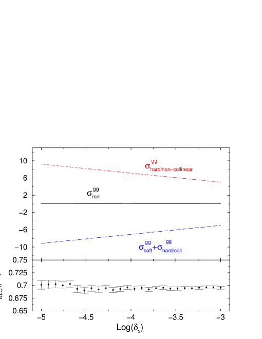
Figure 7: Dependence of $\sigma_{\scriptscriptstyle NLO}(pp\to t\bar{t}h)$ on the soft cutoff $\delta_{s}$ of the two-cutoff PSS method, at $\sqrt{s_{\scriptscriptstyle H}}\!=\!14$ TeV, for $M_{h}\!=\!120$ GeV, $\mu\!=\!m_{t}+M_{h}/2$, and $\delta_{c}\!=\!10^{-5}$. The upper plot shows the cancellation of the $\delta_{s}$-dependence between $\sigma_{soft}^{gg}+\sigma_{hard/coll}^{gg}$ and $\sigma_{hard/non-coll}^{gg}$. The lower plot shows, on an enlarged scale, the dependence of the full $\sigma_{\scriptscriptstyle NLO}=\sigma_{\scriptscriptstyle NLO}^{gg}+\sigma_{\scriptscriptstyle NLO}^{q\bar{q}}+\sigma_{\scriptscriptstyle NLO}^{qg}$ on $\delta_{s}$ with the corresponding statistical errors.

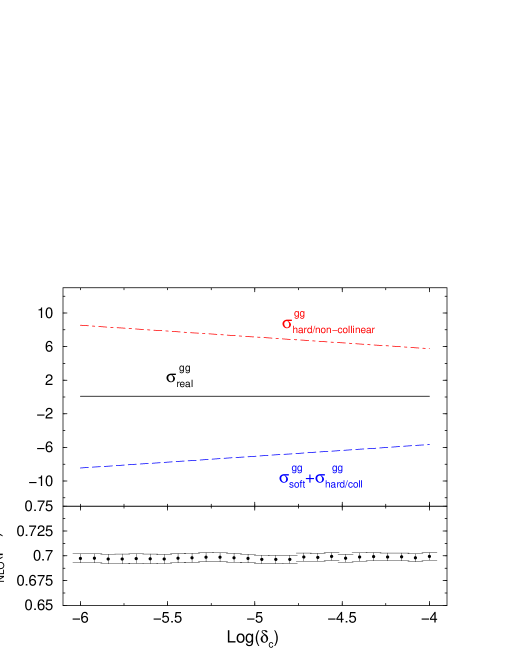
Figure 8: Dependence of $\sigma_{\scriptscriptstyle NLO}(pp\to t\bar{t}h)$ on the collinear cutoff $\delta_{c}$ of the two-cutoff PSS method, at $\sqrt{s_{\scriptscriptstyle H}}\!=\!14$ TeV, for $M_{h}\!=\!120$ GeV, $\mu\!=\!m_{t}+M_{h}/2$, and $\delta_{s}\!=\!10^{-4}$. The upper plot shows the cancellation of the $\delta_{s}$-dependence between $\sigma_{soft}^{gg}+\sigma_{hard/coll}^{gg}$, and $\sigma_{hard/non-coll}^{gg}$. The lower plot shows, on an enlarged scale, the dependence of the full $\sigma_{\scriptscriptstyle NLO}=\sigma_{\scriptscriptstyle NLO}^{gg}+\sigma_{\scriptscriptstyle NLO}^{q\bar{q}}+\sigma_{\scriptscriptstyle NLO}^{qg}$ on $\delta_{c}$ with the corresponding statistical errors.

We now turn to the one-cutoff PSS method and, following the same criterion adopted for the case of the two-cutoff PSS method, we summarize in the upper window of Fig. 9 the behavior of the different cutoff dependent contributions to the real $gg\to t\bar{t}h$ cross section, i.e. $\sigma_{ir}^{gg}$ and $\sigma_{hard}^{gg}$, as well as the resulting cutoff independence of $\sigma_{real}^{gg}$. The lower window of Fig. 9 shows the full $\sigma_{\scriptscriptstyle NLO}$, where all $t\bar{t}h$ subprocesses are included, on an enlarged scale. The statistical deviations due to the Monte Carlo integration are also shown, and therefore the stability of the integration procedure can be appreciated. In Fig. 9 $s_{min}$ is varied over several orders of magnitude and the presence of a clear plateau over most of the $s_{min}$ range is evident. The results presented in Section VII have been cross-checked using the one-cutoff PSS method with $s_{min}\!=\!10$ GeV².

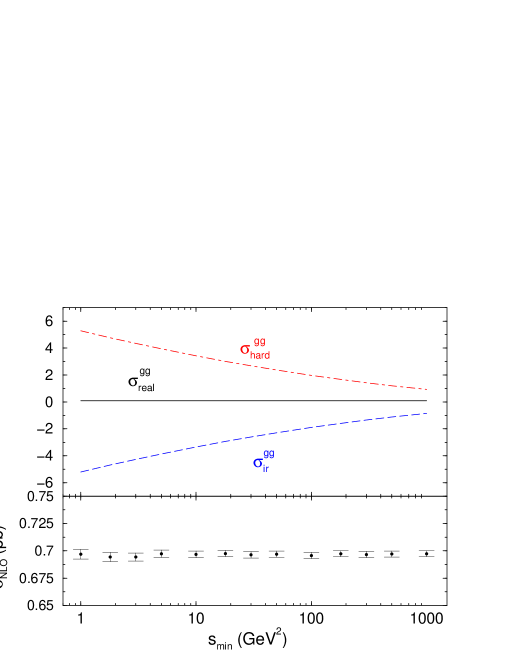
Figure 9: Dependence of $\sigma_{\scriptscriptstyle NLO}(pp\to t\bar{t}h)$ on the $s_{min}$ cutoff of the one-cutoff PSS method, at $\sqrt{s_{\scriptscriptstyle H}}\!=\!14$ TeV, for $M_{h}\!=\!120$ GeV, and $\mu\!=\!m_{t}+M_{h}/2$. The upper plot shows the cancellation of the $s_{min}$-dependence between $\sigma_{ir}^{gg}$ and $\sigma_{hard}^{gg}$. The lower plot shows, on an enlarged scale, the dependence of the full $\sigma_{\scriptscriptstyle NLO}=\sigma_{\scriptscriptstyle NLO}^{gg}+\sigma_{\scriptscriptstyle NLO}^{q\bar{q}}+\sigma_{\scriptscriptstyle NLO}^{qg}$ on $s_{min}$ with the corresponding statistical errors.

VII Numerical results

In this section we summarize the most important numerical results for $\sigma_{\scriptscriptstyle NLO}(pp\to t\bar{t}h)$ and illustrate the impact of NLO QCD corrections on the tree level cross section. In particular, we discuss the renormalization/factorization scale dependence of $\sigma_{\scriptscriptstyle NLO}$ with respect to $\sigma_{\scriptscriptstyle LO}$, and illustrate the dependence of both LO and NLO cross sections on the Higgs boson mass. Results for $\sigma_{\scriptscriptstyle LO}$ are obtained using the 1-loop evolution of $\alpha_{s}(\mu)$ and CTEQ5L parton distribution functions Lai et al. (2000), while results for $\sigma_{\scriptscriptstyle NLO}$ are obtained using the 2-loop evolution of $\alpha_{s}(\mu)$ and CTEQ5M parton distribution functions, with $\alpha_{s}^{\scriptscriptstyle NLO}(M_{Z})\!=\!0.118$. According to the renormalization prescription adopted in this paper and explained in Section IV.1, throughout our calculation we use for the input parameter $m_{t}$ the top quark pole mass. Results are presented for $m_{t}\!=\!174$ GeV, while the uncertainty introduced by varying $m_{t}$ within its experimental uncertainty is discussed later in this section. We define the top quark Yukawa coupling to be $g_{t\bar{t}h}\!=\!m_{t}/v$ where $v\!=(G_{F}\sqrt{2})^{-1/2}\!=\!246$ GeV is the vacuum expectation value of the SM Higgs field, given in terms of the Fermi constant $G_{F}$.

In Fig. 10, we illustrate the dependence of both $\sigma_{\scriptscriptstyle NLO}$ and $\sigma_{\scriptscriptstyle LO}$ on the renormalization and factorization scales when the two scales are identical, i.e. when $\mu_{r}\!=\!\mu_{f}\!=\!\mu$. We have also studied the behavior of $\sigma_{\scriptscriptstyle NLO}$ when the renormalization and factorization scales are varied independently and noticed no appreciable difference with respect to the case in which the two scales are identical. This justifies our decision to present results only for $\mu_{r}\!=\!\mu_{f}\!=\!\mu$. We also illustrate in Fig. 11 the $\mu$ dependence of the NLO cross section for each parton level channel independently. We use $M_{h}\!=\!120$ GeV for the purpose of these plots. As expected, Fig. 10 shows that the NLO cross section has a much weaker scale dependence and represents a much more stable theoretical prediction.

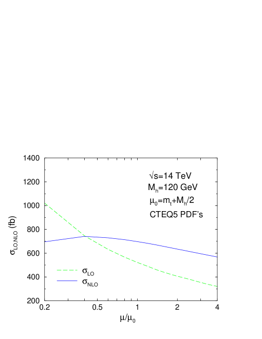
Figure 10: Dependence of $\sigma_{\scriptscriptstyle LO,NLO}(pp\to t\bar{t}h)$ on the renormalization/factorization scale $\mu$, at $\sqrt{s_{\scriptscriptstyle H}}\!=\!14$ TeV, for $M_{h}\!=\!120$ GeV.

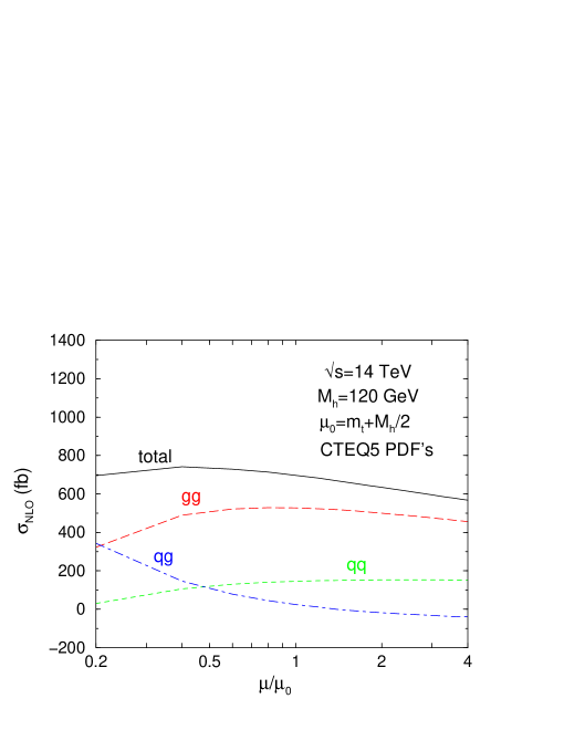
Figure 11: Dependence of $\sigma_{\scriptscriptstyle NLO}(gg,q\bar{q},qg+\bar{q}g\to t\bar{t}h)$ on the renormalization/factorization scale $\mu$, at $\sqrt{s_{\scriptscriptstyle H}}\!=\!14$ TeV, for $M_{h}\!=\!120$ GeV.

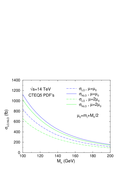
Figure 12: $\sigma_{\scriptscriptstyle NLO}(pp\to t\bar{t}h)$ and $\sigma_{\scriptscriptstyle LO}(pp\to t\bar{t}h)$ as functions of $M_{h}$, at $\sqrt{s_{\scriptscriptstyle H}}\!=\!14$ TeV, for $\mu\!=m_{t}+M_{h}/2$ and $\mu\!=\!2m_{t}+M_{h}$.

In Fig. 12, we plot $\sigma_{\scriptscriptstyle LO}(pp\to t\bar{t}h)$ and $\sigma_{\scriptscriptstyle NLO}(pp\to t\bar{t}h)$ as functions of the Higgs boson mass, for $\sqrt{s_{\scriptscriptstyle H}}\!=\!14$ TeV and two values of the common renormalization/factorization scale, $\mu\!=\!m_{t}+M_{h}/2$ and $\mu\!=\!2m_{t}+M_{h}$. We consider $100\,\mbox{GeV}\!\leq\!M_{h}\!\leq\!200\,\mbox{GeV}$ since the production of a Higgs boson in association with a pair of top quarks at the LHC will play a crucial role only for relatively light Higgs bosons. The information gathered from this plot nicely complements what has already been shown in Fig. 10. We summarize a sample of results from both Figs. 10 and 12 in Table 1, where we also provide the LO cross section, $\overline{\sigma}_{\scriptscriptstyle LO}$, calculated using the 2-loop evolution of $\alpha_{s}(\mu)$ and CTEQ5M PDFs. This can be useful to separately evaluate the impact of the full set of NLO QCD corrections as opposed to the subset of them that mainly correspond to the NLO running of $\alpha_{s}(\mu)$. The error we quote on our values is the statistical error of the numerical integration involved in evaluating the total cross section. We estimate the remaining theoretical uncertainty on the NLO results to be of the order of $15-20\%$. This is mainly due to: the left over $\mu$-dependence (about $15\%$), the dependence on the PDFs (about $6\%$), and the error on $m_{t}$ (about $7\%$) which particularly plays a role in the top quark Yukawa coupling.

$M_{h}$ (GeV)	$\mu$	$\sigma_{\scriptscriptstyle LO}$ (fb)	$\overline{\sigma}_{\scriptscriptstyle LO}$ (fb)	$\sigma_{\scriptscriptstyle NLO}$ (fb)
	$m_{t}$	582.92 $\pm$ 0.06	616.81 $\pm$ 0.07	718.64 $\pm$ 3.71
120	$m_{t}+M_{h}/2$	520.47 $\pm$ 0.06	553.25 $\pm$ 0.06	697.27 $\pm$ 3.20
	$2m_{t}$	450.09 $\pm$ 0.05	480.80 $\pm$ 0.05	662.66 $\pm$ 2.77
	$2m_{t}+M_{h}$	405.54 $\pm$ 0.04	434.59 $\pm$ 0.05	634.36 $\pm$ 2.34
	$m_{t}$	316.27 $\pm$ 0.03	336.41 $\pm$ 0.04	380.95 $\pm$ 1.81
150	$m_{t}+M_{h}/2$	275.44 $\pm$ 0.03	294.35 $\pm$ 0.03	367.38 $\pm$ 1.52
	$2m_{t}$	243.47 $\pm$ 0.03	261.03 $\pm$ 0.03	352.71 $\pm$ 1.35
	$2m_{t}+M_{h}$	214.43 $\pm$ 0.02	230.60 $\pm$ 0.02	334.48 $\pm$ 1.18
	$m_{t}$	187.44 $\pm$ 0.02	200.46 $\pm$ 0.02	221.63 $\pm$ 1.01
180	$m_{t}+M_{h}/2$	159.32 $\pm$ 0.02	171.15 $\pm$ 0.02	214.01 $\pm$ 0.85
	$2m_{t}$	143.77 $\pm$ 0.02	154.74 $\pm$ 0.02	206.59 $\pm$ 0.77
	$2m_{t}+M_{h}$	123.85 $\pm$ 0.01	133.65 $\pm$ 0.02	194.42 $\pm$ 0.70

Table 1: Values of both $\sigma_{\scriptscriptstyle LO}(pp\to t\bar{t}h)$, $\overline{\sigma}_{\scriptscriptstyle LO}(pp\to t\bar{t}h)$, and $\sigma_{\scriptscriptstyle NLO}(pp\to t\bar{t}h)$, at $\sqrt{s_{\scriptscriptstyle H}}\!=\!14$ TeV, for a sample of different values of $M_{h}$ and of the renormalization/factorization scales $\mu\!=\!\mu_{r}\!=\!\mu_{f}$.

It can also be useful to quote the impact of NLO corrections in terms of a so called $K$-factor, defined as the ratio between the NLO and LO cross sections:

$$K=\frac{\sigma_{\scriptscriptstyle NLO}(pp\to t\bar{t}h)}{\sigma_{\scriptscriptstyle LO}(pp\to t\bar{t}h)}\,\,\,.$$ (94)

We can see in Fig. 10 that, for a SM Higgs boson of mass $M_{h}\!=\!120$ GeV, the $K$-factor for $pp\to t\bar{t}h$ is larger than unity when $\mu\!\geq\!0.4\mu_{0}$ for $\mu_{0}\!=\!m_{t}+M_{h}/2$. Therefore, over a broad range of the commonly used renormalization/factorization scales, NLO QCD corrections increase the LO cross section. Using the results of Table 1, the K-factors for a sample of Higgs boson masses and renormalization/factorization scales can easily be calculated, both using $\sigma_{\scriptscriptstyle LO}$ and $\overline{\sigma}_{\scriptscriptstyle LO}$. We notice, however, that the $K$-factor defined in Eq. (94) is affected by a very strong scale dependence, the same as $\sigma_{\scriptscriptstyle LO}$. Therefore, when the $K$-factor is used to obtain $\sigma_{\scriptscriptstyle NLO}$ from $\sigma_{\scriptscriptstyle LO}$, care must be used in matching $\sigma_{\scriptscriptstyle LO}$ and $K$ corresponding to the same $\mu$-scale.

VIII Conclusions

The associated production of a Higgs boson with a pair of top quarks will play a very important role in the discovery of a low mass Higgs boson at the LHC with a center of mass energy of $\sqrt{s_{\scriptscriptstyle H}}\!=\!14$ TeV. With the statistics expected at the LHC, $pp\to t\bar{t}h$, with $h\to b\bar{b},\tau^{+}\tau^{-},W^{+}W^{-},\gamma\gamma$ will also play a crucial role in determining the couplings of the discovered Higgs boson, and will give the only handle on a direct measurement of the top quark Yukawa coupling.

In this paper the inclusive cross section for $pp\to t\bar{t}h$ production has been calculated, in the Standard Model, including full NLO QCD corrections. The NLO cross section shows a drastically reduced renormalization and factorization scale dependence, and leads to increased confidence in predictions based on these results. The overall uncertainty on the theoretical prediction, including the errors coming from parton distribution functions and the top quark mass, is reduced to only 15-20%, as opposed to the 100-200% uncertainty of the LO cross section. Including NLO QCD corrections increases the LO cross section for a broad range of commonly used renormalization and factorization scales, and over the entire Higgs boson mass range considered in this paper. This is summarized by saying that the $K$-factor for renormalization and factorization scales in the range $m_{t}\!<\!\mu\!\leq\!2m_{t}+M_{h}$ and Higgs boson masses in the range $100\,\mbox{GeV}\!\leq M_{h}\!\leq\!200\,\mbox{GeV}$ is between 1.2 and 1.6.

The calculation of the NLO QCD cross section for $pp\to t\bar{t}h$ contains several technical difficulties that have been thoroughly explained in this paper (see also Ref. Reina et al. (2002)). The NLO virtual corrections involve pentagon diagrams and consequently require the evaluation of both scalar and tensor pentagon integrals with several external and internal massive particles. Detailed information about the method used as well as explicit results for all the IR singular integrals appearing in the calculation are presented in a series of Appendices. Tensor pentagon integrals are affected by numerical instabilities and we discuss in this paper how we have calculated them in a numerically stable form. The NLO real corrections are complicated by the presence of IR divergences. We have calculated them in two different variations of the phase space slicing method, involving one or two arbitrary cutoffs respectively. The correspondence between the two phase space slicing methods is made explicit, and the agreement between them constitutes a powerful check of the technicalities used in their implementations. The techniques developed in this paper and in Ref. Reina et al. (2002) can now be applied to similar higher order calculations, in particular to the case of the associated $b\bar{b}h$ production at both the Tevatron and the LHC.

Appendix A Tree level amplitude for $gg\to t\bar{t}h$

The amplitudes ${\cal A}_{0,s}$, ${\cal A}_{0,t}$, and ${\cal A}_{0,u}$ introduced in Section II can be written as:

$${\cal A}_{0,s} = ig_{s}^{2}\,g_{t\bar{t}h}\,\epsilon_{\mu}(q_{1})\,\epsilon_{\nu}(q_{2})\,\bar{u}_{t}{\cal A}_{0,s}^{\mu\nu}v_{\bar{t}}\,\,\,,$$

$${\cal A}_{0,t} = ig_{s}^{2}\,g_{t\bar{t}h}\,\epsilon_{\mu}(q_{1})\,\epsilon_{\nu}(q_{2})\,\bar{u}_{t}{\cal A}_{0,t}^{\mu\nu}v_{\bar{t}}\,\,\,,$$

$${\cal A}_{0,u} = ig_{s}^{2}\,g_{t\bar{t}h}\,\epsilon_{\mu}(q_{1})\,\epsilon_{\nu}(q_{2})\,\bar{u}_{t}{\cal A}_{0,u}^{\mu\nu}v_{\bar{t}}\,\,\,,$$ (95)

where $g_{t\bar{t}h}\!=\!m_{t}/v$ is the top quark Yukawa coupling, with $v\!=\!246$ GeV the SM Higgs boson vacuum expectation value, while ${\cal A}_{0,s}^{\mu\nu}$, ${\cal A}_{0,t}^{\mu\nu}$, and ${\cal A}_{0,u}^{\mu\nu}$ represent the total $s-$channel, $t-$channel, and $u-$channel amplitudes, corresponding to the diagrams in Fig. 1. More explicitly:

$${\cal A}_{0,s}^{\mu\nu} = {\cal A}_{0,s}^{(1)\mu\nu}+{\cal A}_{0,s}^{(2)\mu\nu}\,\,\,,$$

$${\cal A}_{0,t}^{\mu\nu} = {\cal A}_{0,t}^{(1)\mu\nu}+{\cal A}_{0,t}^{(2)\mu\nu}+{\cal A}_{0,t}^{(3)\mu\nu}\,\,\,,$$

$${\cal A}_{0,u}^{\mu\nu} = {\cal A}_{0,u}^{(1)\mu\nu}+{\cal A}_{0,u}^{(2)\mu\nu}+{\cal A}_{0,u}^{(3)\mu\nu}\,\,\,,$$ (96)

where

$${\cal A}_{0,s}^{(1),\mu\nu} = \frac{1}{s}\frac{\not p_{t}+\not p_{h}+m_{t}}{[(p_{t}+p_{h})^{2}-m_{t}^{2}]}\gamma_{\alpha}V^{\mu\nu\alpha}\,\,\,,$$

$${\cal A}_{0,s}^{(2),\mu\nu} = \frac{1}{s}\gamma_{\alpha}\frac{-\not p_{t}^{\prime}-\not p_{h}+m_{t}}{[(p_{t}^{\prime}+p_{h})^{2}-m_{t}^{2}]}V^{\mu\nu\alpha}\,\,\,,$$

$${\cal A}_{0,t}^{(1),\mu\nu} = \frac{\not p_{t}+\not p_{h}+m_{t}}{[(p_{t}+p_{h})^{2}-m_{t}^{2}]}\gamma^{\mu}\frac{\not q_{2}-\not p_{t}^{\prime}+m_{t}}{[(q_{2}-p_{t}^{\prime})^{2}-m_{t}^{2}]}\gamma^{\nu}\,\,\,,$$

$${\cal A}_{0,t}^{(2),\mu\nu} = \gamma_{\mu}\frac{\not p_{t}-\not q_{1}+m_{t}}{[(p_{t}-q_{1})^{2}-m_{t}^{2}]}\frac{\not q_{2}-\not p_{t}^{\prime}+m_{t}}{[(q_{2}-p_{t}^{\prime})^{2}-m_{t}^{2}]}\gamma_{\nu}\,\,\,,$$

$${\cal A}_{0,t}^{(3),\mu\nu} = \gamma_{\mu}\frac{\not p_{t}-\not q_{1}+m_{t}}{[(p_{t}-q_{1})^{2}-m_{t}^{2}]}\gamma^{\nu}\frac{-\not p_{t}^{\prime}-\not p_{h}+m_{t}}{[(p_{t}^{\prime}+p_{h})^{2}-m_{t}^{2}]}\,\,\,,$$

$${\cal A}_{0,u}^{(1),\mu\nu} = {\cal A}_{0,t}^{(1),\mu\nu}(\mu\leftrightarrow\nu,q_{1}\leftrightarrow q_{2})\,\,\,,$$

$${\cal A}_{0,u}^{(2),\mu\nu} = {\cal A}_{0,t}^{(2),\mu\nu}(\mu\leftrightarrow\nu,q_{1}\leftrightarrow q_{2})\,\,\,,$$

$${\cal A}_{0,u}^{(3),\mu\nu} = {\cal A}_{0,t}^{(3),\mu\nu}(\mu\leftrightarrow\nu,q_{1}\leftrightarrow q_{2})\,\,\,,$$ (97)

with

$$V^{\mu\nu\alpha}=(q_{1}-q_{2})^{\alpha}g^{\mu\nu}+(q_{1}+2q_{2})^{\mu}g^{\nu\alpha}-(2q_{1}+q_{2})^{\nu}g^{\mu\alpha}\,\,\,,$$

are the individual amplitudes for the $s-$channel, $t-$channel, and $u-$channel diagrams in Fig. 1.

Appendix B Box and Pentagon integrals

We label the various one-loop box and pentagon scalar and tensor integrals appearing in the calculation of the ${\cal O}(\alpha_{s})$ virtual corrections to

$$g(q_{1})+g(q_{2})\rightarrow t(p_{t})+\bar{t}(p_{t}^{\prime})+h(p_{h})$$

according to the diagram where they are encountered. Moreover we denote by $D0$, $D1^{\mu}$, $D2^{\mu\nu}$, and $D3^{\mu\nu\rho}$ the scalar and tensor box integrals with one, two, and three tensor indices, and by $E0$, $E1^{\mu}$, $E2^{\mu\nu}$, and $E3^{\mu\nu\rho}$ the analogous scalar and tensor pentagon integrals. With this convention $D0_{D_{i,j}^{(k)}}$, for instance, is the scalar box integral appearing in box diagram $D_{i,j}^{(k)}$, as labeled in Fig. 4. The external momenta are labeled as shown above, where $q_{1},q_{2}$ are incoming and $p_{t},p_{t}^{\prime},p_{h}$ are outgoing momenta with $q_{1}+q_{2}=p_{t}+p_{t}^{\prime}+p_{h}$. It is convenient to express our results in terms of the kinematic invariants of Eq. (IV.2) and:

$$\omega_{1} = (p_{t}+p_{h})^{2}-m_{t}^{2}\,\,\,,$$

$$\omega_{2} = (p_{t}^{\prime}+p_{h})^{2}-m_{t}^{2}\,\,\,.$$ (98)

These kinematic invariants do not form a linearly independent set, but are related by:

$$\tau_{3}=\sigma-\tau_{1}-\omega_{2}\,\,\,\,\,\,\,\,\,\,\mbox{and}\,\,\,\,\,\,\,\,\,\,\tau_{4}=\sigma-\tau_{2}-\omega_{1}\,\,\,.$$ (99)

We also make frequent use of the shorthand notation $\Lambda_{a}\!\equiv\!\ln(a/m_{t}^{2})$ with $a=\sigma,\tau_{i},\omega_{i}$.

In the following, we explicitly give only the box and pentagon integrals that contain IR divergences. The IR divergences are extracted using dimensional regularization with $d\!=\!4-2\epsilon$. We only give results for integrals arising from the $s-$channel and $t-$channel diagrams. The integrals for the $u-$channel diagrams can be obtained from the integrals of the corresponding $t-$channel diagrams by exchanging $q_{1}\leftrightarrow q_{2}$, i.e. by exchanging $\tau_{1}\leftrightarrow\tau_{3}$ and $\tau_{2}\leftrightarrow\tau_{4}$. The IR finite scalar integrals are evaluated by implementing the method described in Ref. Denner (1993) and are cross checked against the FF package van Oldenborgh and Vermaseren (1990).

B.1 Box integrals

The scalar and tensor box integrals arising in the computation of box diagram $D_{i,j}^{(k)}$ are of the following form:

$$D0_{D_{i,j}^{(k)}},D1_{D_{i,j}^{(k)}}^{\mu},D2_{D_{i,j}^{(k)}}^{\mu\nu},D3_{D_{i,j}^{(k)}}^{\mu\nu\rho}=\mu^{4-d}\int\frac{d^{d}k}{(2\pi)^{d}}\frac{1,k^{\mu},k^{\mu}k^{\nu},k^{\mu}k^{\nu}k^{\rho}}{N_{1}N_{2}N_{3}N_{4}}\,\,\,,$$ (100)

where

$$N_{1}=(k^{2}-m_{0}^{2})\,\,\, \,\,\,N_{2}=(k+p_{1})^{2}-m_{1}^{2}\,\,\,,$$ ,

$$N_{3}=(k+p_{1}+p_{2})^{2}-m_{2}^{2}\,\,\, \,\,\,N_{4}=(k+p_{1}+p_{2}+p_{3})^{2}-m_{3}^{2}\,\,\,,$$ , (101)

$p_{1}$, $p_{2}$, $p_{3}$, and $p_{4}\!=\!-p_{1}-p_{2}-p_{3}$ are the external (incoming) momenta connected to the box topology, and $m_{0}$, $m_{1}$, $m_{2}$, and $m_{3}$ are the masses of the propagators in the box loop. We write the tensor integrals as a linear combination of the linearly independent tensor structures built of the independent external momenta $p_{1}^{\mu}$, $p_{2}^{\mu}$, and $p_{3}^{\mu}$ plus the metric tensor $g^{\mu\nu}$. Our notation for the box tensor integrals is as follows:

$$D1^{\mu} = D_{1}^{(1)}p_{1}^{\mu}+D_{1}^{(2)}p_{2}^{\mu}+D_{1}^{(3)}p_{3}^{\mu}\,\,\,,$$

$$D2^{\mu\nu} = D_{2}^{(0)}g^{\mu\nu}+D_{2}^{(11)}p_{1}^{\mu}p_{1}^{\nu}+D_{2}^{(22)}p_{2}^{\mu}p_{2}^{\nu}+D_{2}^{(33)}p_{3}^{\mu}p_{3}^{\nu}$$

$$+ D_{2}^{(12)}(p_{1}^{\mu}p_{2}^{\nu}+p_{1}^{\nu}p_{2}^{\mu})+D_{2}^{(13)}(p_{1}^{\mu}p_{3}^{\nu}+p_{1}^{\nu}p_{3}^{\mu})+D_{2}^{(23)}(p_{2}^{\mu}p_{3}^{\nu}+p_{2}^{\nu}p_{3}^{\mu})\,\,\,,$$

$$D3^{\mu\nu\rho} = D_{3}^{(01)}(g^{\mu,\nu}p_{1}^{\rho}+\mbox{perm})+D_{3}^{(02)}(g^{\mu,\nu}p_{2}^{\rho}+\mbox{perm})+D_{3}^{(03)}(g^{\mu,\nu}p_{3}^{\rho}+\mbox{perm})$$

$$+ D_{3}^{(111)}p_{1}^{\mu}p_{1}^{\nu}p_{1}^{\rho}+D_{3}^{(222)}p_{2}^{\mu}p_{2}^{\nu}p_{2}^{\rho}+D_{3}^{(333)}p_{3}^{\mu}p_{3}^{\nu}p_{3}^{\rho}$$

$$+ D_{3}^{(112)}(p_{1}^{\mu}p_{1}^{\nu}p_{2}^{\rho}+\mbox{perm})+D_{3}^{(113)}(p_{1}^{\mu}p_{1}^{\nu}p_{3}^{\rho}+\mbox{perm})$$

$$+ D_{3}^{(221)}(p_{2}^{\mu}p_{2}^{\nu}p_{1}^{\rho}+\mbox{perm})+D_{3}^{(223)}(p_{2}^{\mu}p_{2}^{\nu}p_{3}^{\rho}+\mbox{perm})$$

$$+ D_{3}^{(331)}(p_{3}^{\mu}p_{3}^{\nu}p_{1}^{\rho}+\mbox{perm})+D_{3}^{(332)}(p_{3}^{\mu}p_{3}^{\nu}p_{2}^{\rho}+\mbox{perm})+D_{3}^{(123)}(p_{1}^{\mu}p_{2}^{\nu}p_{3}^{\rho}+\mbox{perm})\,\,\,,$$

where “$+\mbox{perm}$” indicates that the sum over all possible permutations of the tensor indices is understood. In the following we will give the full structure of the scalar box integrals, including both pole and finite parts, while for the corresponding tensor integrals we will only give the IR pole parts, since they can be of interest in checking the IR structure of the virtual cross section. We will write the pole part of each tensor integral coefficient as

$$D_{i}^{(j)}|_{IR-pole} = \frac{i}{16\pi^{2}}{\cal N}_{t}\Delta_{IR}(D_{i}^{(j)})\,\,\,,$$

$$D_{i}^{(jk)}|_{IR-pole} = \frac{i}{16\pi^{2}}{\cal N}_{t}\Delta_{IR}(D_{i}^{(jk)})\,\,\,,$$

$$D_{i}^{(jkl)}|_{IR-pole} = \frac{i}{16\pi^{2}}{\cal N}_{t}\Delta_{IR}(D_{i}^{(jkl)})\,\,\,,$$ (103)

where ${\cal N}_{t}$ is defined in Eq. (17), and give for each box integral the non zero $\Delta_{IR}(D_{i}^{(j)})$, $\Delta_{IR}(D_{i}^{(jk)})$, and $\Delta_{IR}(D_{i}^{(jkl)})$ coefficients.

B.1.1 Box scalar integral $D0_{B_{2,s}^{(1,2)}}$

The scalar integral appearing in diagram $B_{2,s}^{(1)}$ can be parameterized according to Eq. (100) with:

$$N_{1}=k^{2}\,\,\, \,\,\,N_{2}=(k+p_{t})^{2}-m_{t}^{2}\,\,\,,$$ ,

$$N_{3}=(k+p_{t}+p_{h})^{2}-m_{t}^{2}\,\,\, \,\,\,N_{4}=(k-p_{t}^{\prime})^{2}-m_{t}^{2}\,\,\,.$$ , (104)

$D0_{B_{2,s}^{(2)}}$ is obtained from $D0_{B_{2,s}^{(1)}}$ by exchanging $p_{t}\leftrightarrow p_{t}^{\prime}$. This integral also appears in the $q\bar{q}\to t\bar{t}h$ calculation and has already been presented in Ref. Reina et al. (2002). We repeat it here for completeness.

The part of $D0_{B_{2,s}^{(1)}}$ which contributes to the amplitude squared is of the form:

$$D0_{B_{2,s}^{(1)}} = \frac{i}{16\pi^{2}}{\cal N}_{t}\,\frac{1}{\omega_{1}(\sigma-\omega_{1}-\omega_{2}+M_{h}^{2})}\left(\frac{X_{-1}}{\epsilon}+X_{0}\right)\,\,\,,$$ (105)

where ${\cal N}_{t}$ is defined in Eq. (17). The pole part $X_{-1}$ is:

$$X_{-1}=-\frac{1}{\beta_{t\bar{t}}}\ln\left(\frac{1+\beta_{t\bar{t}}}{1-\beta_{t\bar{t}}}\right)\,\,\,,$$ (106)

where $\beta_{t\bar{t}}$ is given in Eq. (28). The finite part $X_{0}$ can be calculated using Ref. Beenakker and Denner (1990). All tensor box integrals associated to $B_{2,s}^{(1)}$ and $B_{2,s}^{(2)}$ are IR finite.

B.1.2 Box scalar integral $D0_{B_{7,t}^{(1,2)}}$

The scalar integral appearing in diagram $B_{7,t}^{(1)}$, $D0_{B_{7,t}^{(1)}}$, can be parameterized according to Eq. (100) with:

$$N_{1}=k^{2}\,\,\, \,\,\,N_{2}=(k+q_{1})^{2}\,\,\,,$$ ,

$$N_{3}=(k+q_{1}-p_{t})^{2}-m_{t}^{2}\,\,\, \,\,\,N_{4}=(k+q_{1}-p_{t}-p_{h})^{2}-m_{t}^{2}\,\,\,.$$ , (107)

The part of $D0_{B_{7,t}^{(1)}}$ which contributes to the virtual amplitude squared is of the form:

$$D0_{B_{7,t}^{(1)}}=\frac{i}{16\pi^{2}}{\cal N}_{t}\left(-\frac{1}{\omega_{1}\tau_{1}}\right)\left(\frac{X_{-2}}{\epsilon^{2}}+\frac{X_{-1}}{\epsilon}+X_{0}\right)\,\,\,,$$ (108)

where the coefficients $X_{-2}$, $X_{-1}$, and $X_{0}$ are given by:

$$X_{-2} = \frac{1}{2}\,\,\,,$$

$$X_{-1} = \ln\left(\frac{\tau_{2}m_{t}^{2}}{\omega_{1}\tau_{1}}\right)\,\,\,,$$

$$X_{0} = Re\left\{-\frac{5}{6}\pi^{2}+\ln^{2}\left(\frac{\omega_{1}}{m_{t}^{2}}\right)+\ln^{2}\left(\frac{\tau_{1}}{m_{t}^{2}}\right)-\ln^{2}\left(\frac{\tau_{2}}{m_{t}^{2}}\right)\right.$$

$$+ 2\,\ln\left(\frac{\omega_{1}+\tau_{2}}{\tau_{1}}\right)\ln\left(\frac{\tau_{2}}{\omega_{1}}\right)+2\,\ln\left(\frac{\tau_{1}-\tau_{2}}{\omega_{1}}\right)\ln\left(\frac{\tau_{2}}{\tau_{1}}\right)$$

$$- 2\left.\,\mbox{Li}_{2}\left(\frac{\tau_{1}-\tau_{2}-\omega_{1}}{\tau_{1}}\right)-2\,\mbox{Li}_{2}\left(\frac{\omega_{1}+\tau_{2}-\tau_{1}}{\omega_{1}}\right)+2\,\mbox{Li}_{2}\left(\frac{\tau_{2}(\omega_{1}+\tau_{2}-\tau_{1})}{\omega_{1}\tau_{1}}\right)-I_{0}\right\}\,\,\,,$$

with

$$I_{0} = \ln\left(\frac{\tau_{1}}{\tau_{2}}\right)\ln\left(\frac{M_{h}^{2}}{m_{t}^{2}}\right)+\left\{-\mbox{Li}_{2}\left(\frac{1}{\lambda_{+}}\right)+\ln\left(\frac{\tau_{1}}{\tau_{2}}\right)\ln\left(\frac{-\tau_{2}-\lambda_{+}(\tau_{1}-\tau_{2})}{\tau_{1}-\tau_{2}}\right)\right.$$

$$- \left.\mbox{Li}_{2}\left(\frac{\tau_{1}}{\lambda_{+}(\tau_{1}-\tau_{2})+\tau_{2}}\right)+\mbox{Li}_{2}\left(\frac{\tau_{2}}{\lambda_{+}(\tau_{1}-\tau_{2})+\tau_{2}}\right)+(\lambda_{+}\leftrightarrow\lambda_{-})\right\}\,\,\,,$$

and

$$\lambda_{\pm}=\frac{1}{2}\left(1\pm\sqrt{1-\frac{4m_{t}^{2}}{M_{h}^{2}}}\right)\,\,\,.$$ (111)

The tensor integrals associated with $B_{7,t}^{(1)}$ also contain IR divergences. Using the notation introduced in Eqs. (B.1) and (B.1), only the following coefficients of $D1_{B_{7,t}^{(1)}}^{\mu}$:

$$\Delta_{IR}(D_{1}^{(1)}) = \frac{1}{2}\frac{1}{\tau_{1}\omega_{1}}\frac{1}{\epsilon^{2}}+\frac{1}{\tau_{1}\omega_{1}}\left[-\Lambda_{\tau_{1}}+\frac{\tau_{2}}{\tau_{2}+\omega_{1}}\left(\Lambda_{\tau_{2}}-\Lambda_{\omega_{1}}\right)\right]\frac{1}{\epsilon}\;,$$ (112)

and of $D2_{B_{7,t}^{(1)}}^{\mu\nu}$:

$$\Delta_{IR}(D_{2}^{(11)}) = -\frac{1}{2}\frac{1}{\tau_{1}\omega_{1}}\frac{1}{\epsilon^{2}}+\frac{1}{\tau_{1}\omega_{1}}\left[\Lambda_{\tau_{1}}-\frac{\tau_{2}^{2}}{(\tau_{2}+\omega_{1})^{2}}\left(\Lambda_{\tau_{2}}-\Lambda_{\omega_{1}}\right)-\frac{\omega_{1}}{\tau_{2}+\omega_{1}}\right]\frac{1}{\epsilon}\;,$$

are IR divergent.

$D0_{B_{7,t}^{(2)}}$ and the corresponding tensor integrals are obtained from $D0_{B_{7,t}^{(1)}}$ by exchanging $q_{1}\leftrightarrow q_{2}$ and $p_{t}\leftrightarrow p_{t}^{\prime}$, i.e. by exchanging $\tau_{1}\leftrightarrow\tau_{2}$ and $\omega_{1}\leftrightarrow\omega_{2}$ in Eqs. (108)-(B.1.2).

B.1.3 Box scalar integral $D0_{B_{8,t}^{(1,2)}}$

The scalar box integral appearing in diagram $B_{8,t}^{(1)}$, $D0_{B_{8,t}^{(1)}}$, can be parameterized according to Eq. (100) with:

$$N_{1}=k^{2}\,\,\, \,\,\,N_{2}=(k+q_{1})^{2}\,\,\,,$$ ,

$$N_{3}=(k+q_{1}+q_{2})^{2}\,\,\, \,\,\,N_{4}=(k+q_{1}+q_{2}-p_{t}^{\prime})^{2}-m_{t}^{2}\,\,\,.$$ , (114)

The part of $D0_{B_{8,t}^{(1)}}$ which contributes to the virtual amplitude squared is given by:

$$D0_{B_{8,t}^{(1)}} = \frac{i}{16\pi^{2}}{\cal N}_{t}\left(-\frac{1}{\sigma\tau_{2}}\right)\left(\frac{X_{-2}}{\epsilon^{2}}+\frac{X_{-1}}{\epsilon}+X_{0}\right)\,\,\,,$$ (115)

where ${\cal N}_{t}$ is defined in Eq. (17), and the coefficients $X_{-2}$, $X_{-1}$, and $X_{0}$ are given by:

$$X_{-2} = \frac{3}{2}\,\,\,,$$

$$X_{-1} = \ln\left(\frac{\omega_{1}m_{t}^{4}}{\sigma\tau_{2}^{2}}\right)\,\,\,,$$

$$X_{0} = 2\ln\left(\frac{\tau_{2}}{m_{t}^{2}}\right)\ln\left(\frac{\sigma}{m_{t}^{2}}\right)-\ln^{2}\left(\frac{\omega_{1}}{m_{t}^{2}}\right)-2\,\mbox{Li}_{2}\left(1+\frac{\omega_{1}}{\tau_{2}}\right)+\frac{\pi^{2}}{3}\,\,\,.$$ (116)

The tensor integrals associated with $B_{8,t}^{(1)}$ also contain IR divergences. Using the notation introduced in Eqs. (B.1) and (B.1), only the following tensor coefficients of $D1_{B_{8,t}^{(1)}}^{\mu}$:

$$\Delta_{IR}(D_{1}^{(1)}) = \frac{3}{2}\frac{1}{\sigma\tau_{2}}\frac{1}{\epsilon^{2}}-\frac{1}{\sigma\tau_{2}}\left[\Lambda_{\sigma}+\Lambda_{\tau_{2}}+\frac{\omega_{1}}{\tau_{2}+\omega_{1}}\left(\Lambda_{\tau_{2}}-\Lambda_{\omega_{1}}\right)\right]\frac{1}{\epsilon}\,\,\,,$$

$$\Delta_{IR}(D_{1}^{(2)}) = \frac{1}{2}\frac{1}{\sigma\tau_{2}}\frac{1}{\epsilon^{2}}-\frac{1}{\sigma\tau_{2}}\Lambda_{\tau_{2}}\frac{1}{\epsilon}\,\,\,,$$ (117)

of $D2_{B_{8,t}^{(1)}}^{\mu\nu}$:

$$\Delta_{IR}(D_{2}^{(11)}) = -\frac{3}{2}\frac{1}{\sigma\tau_{2}}\frac{1}{\epsilon^{2}}+\frac{1}{\sigma\tau_{2}}\left[-\frac{\tau_{2}}{\tau_{2}+\omega_{1}}+\Lambda_{\sigma}+\Lambda_{\tau_{2}}+\frac{\omega_{1}^{2}}{(\tau_{2}+\omega_{1})^{2}}\left(\Lambda_{\tau_{2}}-\Lambda_{\omega_{1}}\right)\right]\frac{1}{\epsilon}\,\,\,,$$

$$\Delta_{IR}(D_{2}^{(12)}) = -\frac{1}{2}\frac{1}{\sigma\tau_{2}}\frac{1}{\epsilon^{2}}+\frac{1}{\sigma\tau_{2}}\Lambda_{\tau_{2}}\frac{1}{\epsilon}\,\,\,,$$

$$\Delta_{IR}(D_{2}^{(22)}) = -\frac{1}{2}\frac{1}{\sigma\tau_{2}}\frac{1}{\epsilon^{2}}+\frac{1}{\sigma\tau_{2}}(-1+\Lambda_{\tau_{2}})\frac{1}{\epsilon}\;,$$ (118)

and of $D3_{B_{8,t}^{(1)}}^{\mu\nu\rho}$:

$$\Delta_{IR}(D_{3}^{(111)}) = \frac{3}{2}\frac{1}{\sigma\tau_{2}}\frac{1}{\epsilon^{2}}+\frac{1}{2\sigma\tau_{2}}\left[\frac{3\tau_{2}}{\tau_{2}+\omega_{1}}+\frac{2\tau_{2}\omega_{1}}{(\tau_{2}+\omega_{1})^{2}}-2\Lambda_{\sigma}-2\Lambda_{\tau_{2}}\right.$$

$$\left.-\frac{2\omega_{1}^{2}}{(\tau_{2}+\omega_{1})^{3}}\left(\Lambda_{\tau_{2}}-\Lambda_{\omega_{1}}\right)\right]\frac{1}{\epsilon}\,\,\,,$$

$$\Delta_{IR}(D_{3}^{(112)}) = \frac{1}{2}\frac{1}{\sigma\tau_{2}}\frac{1}{\epsilon^{2}}-\frac{1}{\sigma\tau_{2}}\Lambda_{\tau_{2}}\frac{1}{\epsilon}\,\,\,,$$

$$\Delta_{IR}(D_{3}^{(221)}) = \frac{1}{2}\frac{1}{\sigma\tau_{2}}\frac{1}{\epsilon^{2}}+\frac{1}{\sigma\tau_{2}}\left(1-\Lambda_{\tau_{2}}\right)\frac{1}{\epsilon}\,\,\,,$$

$$\Delta_{IR}(D_{3}^{(222)}) = \frac{1}{2}\frac{1}{\sigma\tau_{2}}\frac{1}{\epsilon^{2}}+\frac{1}{\sigma\tau_{2}}\left(\frac{3}{2}-\Lambda_{\tau_{2}}\right)\frac{1}{\epsilon}\;,$$ (119)

are IR divergent.

$D0_{B_{8,t}^{(2)}}$ as well as the corresponding tensor integrals can be obtained from $D0_{B_{8,t}^{(1)}}$ by exchanging $q_{1}\leftrightarrow q_{2}$ and $p_{t}^{\prime}\leftrightarrow p_{t}$, i.e. by exchanging $\tau_{1}\leftrightarrow\tau_{2}$ and $\omega_{1}\leftrightarrow\omega_{2}$ in Eqs. (115)-(B.1.3).

B.1.4 Box scalar integral $D0_{B_{10,t}^{(1,2)}}$

The scalar box integral appearing in diagram $B_{10,t}^{(1)}$, $D0_{B_{10,t}}^{(1)}$, can be parameterized according to Eq. 100 with:

$$N_{1}=k^{2}\,\,\, \,\,\,N_{2}=(k+q_{1})^{2}\,\,\,,$$ ,

$$N_{3}=(k+q_{1}-p_{t}^{\prime})^{2}-m_{t}^{2}\,\,\, \,\,\,N_{4}=(k+q_{1}+q_{2}-p_{t}^{\prime})^{2}-m_{t}^{2}\,\,\,.$$ , (120)

The part of $D0_{B_{10,t}^{(1)}}$ which contributes to the virtual amplitude squared is given by:

$$D0_{B_{10,t}}^{(1)} = \frac{i}{16\pi^{2}}{\cal N}_{t}\left(\frac{1}{\tau_{2}\tau_{4}}\right)\left(\frac{X_{-2}}{\epsilon^{2}}+\frac{X_{-1}}{\epsilon}+X_{0}\right)\,\,\,,$$ (121)

where the coefficients $X_{-2}$, $X_{-1}$, and $X_{0}$ are given by:

$$X_{-2} = \frac{1}{2}\,\,\,,$$

$$X_{-1} = \ln\left(\frac{\omega_{1}}{\tau_{4}}\right)-\ln\left(\frac{\tau_{2}}{m_{t}^{2}}\right)\,\,\,,$$

$$X_{0} = {\cal R}e\left\{\ln^{2}\left(\frac{\tau_{2}}{m_{t}^{2}}\right)+\ln^{2}\left(\frac{\tau_{4}}{m_{t}^{2}}\right)-\ln^{2}\left(\frac{\omega_{1}}{m_{t}^{2}}\right)+\frac{3}{2}\pi^{2}\right.$$

$$+ 2\ln\left(\frac{\tau_{2}+\omega_{1}}{\tau_{4}}\right)\ln\left(\frac{\tau_{4}}{\tau_{2}+\tau_{4}+\omega_{1}}\right)+2\ln\left(\frac{\tau_{4}+\omega_{1}}{\tau_{2}}\right)\ln\left(\frac{\tau_{2}}{\tau_{2}+\tau_{4}+\omega_{1}}\right)$$

$$- 2\left.\,\mbox{Li}_{2}\left(\frac{\tau_{2}+\tau_{4}+\omega_{1}}{\tau_{4}}\right)-2\,\mbox{Li}_{2}\left(\frac{\tau_{2}+\tau_{4}+\omega_{1}}{\tau_{2}}\right)-2\,\mbox{Li}_{2}\left(\frac{(\tau_{2}+\omega_{1})(\tau_{4}+\omega_{1})}{\tau_{2}\tau_{4}}\right)\right\}\,\,\,.$$

The tensor integrals associated with $B_{10,t}^{(1)}$ also contain IR divergences. Using the notation introduced in Eqs. (B.1) and (B.1), the only IR divergent tensor coefficients of $D1_{B_{10,t}^{(1)}}^{\mu}$:

$$\Delta_{IR}(D_{1}^{(1)}) = -\frac{1}{2}\frac{1}{\tau_{2}\tau_{4}}\frac{1}{\epsilon^{2}}+\frac{1}{\tau_{2}\tau_{4}(\tau_{2}+\omega_{1})}\left[(\tau_{2}+\omega_{1})\Lambda_{\tau_{4}}+\omega_{1}\left(\Lambda_{\tau_{2}}-\Lambda_{\omega_{1}}\right)\right]\frac{1}{\epsilon}\,\,\,,$$

of $D2_{B_{10,t}^{(1)}}^{\mu\nu}$:

$$\Delta_{IR}(D_{2}^{(11)}) = \frac{1}{2}\frac{1}{\tau_{2}\tau_{4}}\frac{1}{\epsilon^{2}}+\frac{1}{\tau_{2}\tau_{4}(\tau_{2}+\omega_{1})^{2}}\left[\tau_{2}(\tau_{2}+\omega_{1})-(\tau_{2}+\omega_{1})^{2}\Lambda_{\tau_{4}}-\omega_{1}^{2}\left(\Lambda_{\tau_{2}}-\Lambda_{\omega_{1}}\right)\right]\frac{1}{\epsilon}\;,$$

and of $D3_{B_{10,t}^{(1)}}^{\mu\nu\rho}$:

$$\Delta_{IR}(D_{3}^{(111)}) = -\frac{1}{2}\frac{1}{\tau_{2}\tau_{4}}\frac{1}{\epsilon^{2}}-\frac{1}{2}\frac{1}{\tau_{2}\tau_{4}(\tau_{2}+\omega_{1})^{3}}\left[-2\omega_{1}^{2}\left(\Lambda_{\tau_{2}}-\Lambda_{\omega_{1}}\right)-2(\tau_{2}+\omega_{1})^{3}\Lambda_{\tau_{4}}\right.$$ (125)

$$+\left.3\tau_{2}(\tau_{2}+\omega_{1})^{2}+2\tau_{2}\omega_{1}(\tau_{2}+\omega_{1})\right]\frac{1}{\epsilon}\;,$$

are IR divergent.

$D0_{B_{10,t}^{(2)}}$ can be obtained from $D0_{B_{10,t}^{(1)}}$ by exchanging $p_{t}^{\prime}\leftrightarrow p_{t}$, i.e. by exchanging $\tau_{1}\leftrightarrow\tau_{4}$, $\tau_{2}\leftrightarrow\tau_{3}$, and $\omega_{1}\leftrightarrow\omega_{2}$ in Eqs (121) and (125).

B.2 Pentagon integrals

The scalar and tensor pentagon integrals originating from the generic pentagon diagram $P_{i,j}$ in Fig. 5 are of the form:

$$E0_{P_{i,j}},E1_{P_{i,j}}^{\mu},E2_{P_{i,j}}^{\mu\nu},E3_{P_{i,j}}^{\mu\nu\rho}=\mu^{4-d}\int\frac{d^{d}k}{(2\pi)^{d}}\frac{1,k^{\mu},k^{\mu}k^{\nu},k^{\mu}k^{\nu}k^{\rho}}{N_{1}N_{2}N_{3}N_{4}N_{5}}\,\,\,,$$ (126)

where

$$N_{1}=(k^{2}-m_{0}^{2})\,\,\, \,\,\,N_{2}=(k+p_{1})^{2}-m_{1}^{2}\,\,\,,$$ ,

$$N_{3}=(k+p_{1}+p_{2})^{2}-m_{2}^{2}\,\,\, \,\,\,N_{4}=(k+p_{1}+p_{2}+p_{3})^{2}-m_{3}^{2}\,\,\,,$$ ,

$$N_{5}=(k+p_{1}+p_{2}+p_{3}+p_{4})^{2}-m_{4}^{2}\,\,\,$$ , (127)

$p_{1}$, $p_{2}$, $p_{3}$, $p_{4}$, and $p_{5}\!=\!-p_{1}-p_{2}-p_{3}-p_{4}$ are the external (incoming) momenta connected to the pentagon topology, while $m_{0}$, $m_{1}$, $m_{2}$, $m_{3}$, and $m_{4}$ are the masses of the propagators in the pentagon loop.

The scalar pentagon integrals are evaluated as a linear combination of five scalar box integrals, using the technique originally proposed in Ref. Bern et al. (1993, 1994). In particular, we use:

$$E0_{P_{i,j}}=-\frac{1}{2}\sum_{k=1}^{5}c_{k}D0_{P_{i,j}}^{(k)}\,\,\,,$$ (128)

where each scalar box integral $D0_{P_{i,j}}^{(k)}$ can be obtained from the scalar pentagon integral $E0_{P_{i,j}}$ in Eq. (126) by dropping one of the internal propagators. The coefficients $c_{k}$ are given by:

$$c_{k}=\sum_{l=1}^{5}S_{kl}^{-1}\,\,\,,$$ (129)

where $S_{kl}$ is the symmetric matrix:

$$S_{kl}=\frac{1}{2}\left(M_{k}^{2}+M_{l}^{2}-p_{kl}^{2}\right)\,\,\,,$$ (130)

built out of the internal propagator masses $M_{k}$ and $M_{l}$ and the linear combination of external momenta $p_{kl}^{\mu}\!=\!p_{k}^{\mu}+\ldots+p_{l-1}^{\mu}$ ($k,l=1,\ldots,5$). A thorough explanation of this method is given in Ref. Reina et al. (2002); Bern et al. (1993, 1994), to which we refer for more details.

We write the tensor pentagon integrals as a linear combination of the linearly independent tensor structures built of the external momenta $p_{1}^{\mu}$, $p_{2}^{\mu}$, $p_{3}^{\mu}$, and $p_{4}^{\mu}$, which in $d=4$ constitute a complete basis. Our notation for the pentagon tensor integrals is as follows:

$$E1^{\mu} = E_{1}^{(1)}p_{1}^{\mu}+E_{1}^{(2)}p_{2}^{\mu}+E_{1}^{(3)}p_{3}^{\mu}+E_{1}^{(4)}p_{4}^{\mu}\,\,\,,$$

$$E2^{\mu\nu} = E_{2}^{(11)}p_{1}^{\mu}p_{1}^{\nu}+E_{2}^{(22)}p_{2}^{\mu}p_{2}^{\nu}+E_{2}^{(33)}p_{3}^{\mu}p_{3}^{\nu}+E_{2}^{(44)}p_{4}^{\mu}p_{4}^{\nu}$$

$$+ E_{2}^{(12)}(p_{1}^{\mu}p_{2}^{\nu}+p_{1}^{\nu}p_{2}^{\mu})+E_{2}^{(13)}(p_{1}^{\mu}p_{3}^{\nu}+p_{1}^{\nu}p_{3}^{\mu})+E_{2}^{(14)}(p_{1}^{\mu}p_{4}^{\nu}+p_{1}^{\nu}p_{4}^{\mu})$$

$$+ E_{2}^{(23)}(p_{2}^{\mu}p_{3}^{\nu}+p_{2}^{\nu}p_{3}^{\mu})+E_{2}^{(24)}(p_{2}^{\mu}p_{4}^{\nu}+p_{2}^{\nu}p_{4}^{\mu})+E_{2}^{(34)}(p_{3}^{\mu}p_{4}^{\nu}+p_{3}^{\nu}p_{4}^{\mu})\,\,\,,$$

$$E3^{\mu\nu\rho} = E_{3}^{(111)}p_{1}^{\mu}p_{1}^{\nu}p_{1}^{\rho}+E_{3}^{(222)}p_{2}^{\mu}p_{2}^{\nu}p_{2}^{\rho}+E_{3}^{(333)}p_{3}^{\mu}p_{3}^{\nu}p_{3}^{\rho}+E_{3}^{(444)}p_{4}^{\mu}p_{4}^{\nu}p_{4}^{\rho}$$

$$+ E_{3}^{(112)}(p_{1}^{\mu}p_{1}^{\nu}p_{2}^{\rho}+\mbox{perm})+E_{3}^{(113)}(p_{1}^{\mu}p_{1}^{\nu}p_{3}^{\rho}+\mbox{perm})+E_{3}^{(114)}(p_{1}^{\mu}p_{1}^{\nu}p_{4}^{\rho}+\mbox{perm})$$

$$+ E_{3}^{(221)}(p_{2}^{\mu}p_{2}^{\nu}p_{1}^{\rho}+\mbox{perm})+E_{3}^{(223)}(p_{2}^{\mu}p_{2}^{\nu}p_{3}^{\rho}+\mbox{perm})+E_{3}^{(224)}(p_{2}^{\mu}p_{2}^{\nu}p_{4}^{\rho}+\mbox{perm})$$

$$+ E_{3}^{(331)}(p_{3}^{\mu}p_{3}^{\nu}p_{1}^{\rho}+\mbox{perm})+E_{3}^{(332)}(p_{3}^{\mu}p_{3}^{\nu}p_{2}^{\rho}+\mbox{perm})+E_{3}^{(334)}(p_{3}^{\mu}p_{3}^{\nu}p_{4}^{\rho}+\mbox{perm})$$

$$+ E_{3}^{(441)}(p_{4}^{\mu}p_{4}^{\nu}p_{1}^{\rho}+\mbox{perm})+E_{3}^{(442)}(p_{4}^{\mu}p_{4}^{\nu}p_{2}^{\rho}+\mbox{perm})+E_{3}^{(443)}(p_{4}^{\mu}p_{4}^{\nu}p_{4}^{\rho}+\mbox{perm})$$

$$+ E_{3}^{(123)}(p_{1}^{\mu}p_{2}^{\nu}p_{3}^{\rho}+\mbox{perm})+E_{3}^{(124)}(p_{1}^{\mu}p_{2}^{\nu}p_{4}^{\rho}+\mbox{perm})+E_{3}^{(134)}(p_{1}^{\mu}p_{3}^{\nu}p_{4}^{\rho}+\mbox{perm})$$

$$+ E_{3}^{(234)}(p_{2}^{\mu}p_{3}^{\nu}p_{4}^{\rho}+\mbox{perm})\,\,\,.$$

The calculation of $gg\to t\bar{t}h$ involves the six pentagon structures illustrated in Fig. 5. For each of them we will give in the following the IR pole parts of the corresponding scalar integrals, as well as the coefficient $c_{k}$ (in terms of the $S_{kl}$ matrix) and the IR singular box scalar integrals $D0_{P_{i,j}}^{(k)}$ out of which they can be calculated. We will moreover list the IR pole parts of the corresponding tensor integral coefficients, since they may be of interest in checking the IR structure of the virtual cross section. We will write the pole part of each tensor integral coefficient as

$$E_{i}^{(j)}|_{IR-pole} = \frac{i}{16\pi^{2}}{\cal N}_{t}\Delta_{IR}(E_{i}^{(j)})\,\,\,,$$

$$E_{i}^{(jk)}|_{IR-pole} = \frac{i}{16\pi^{2}}{\cal N}_{t}\Delta_{IR}(E_{i}^{(jk)})\,\,\,,$$

$$E_{i}^{(jkl)}|_{IR-pole} = \frac{i}{16\pi^{2}}{\cal N}_{t}\Delta_{IR}(E_{i}^{(jkl)})\,\,\,,$$ (132)

where ${\cal N}_{t}$ is defined in Eq. (17), and give for each pentagon integral the non zero $\Delta_{IR}(E_{i}^{(j)})$, $\Delta_{IR}(E_{i}^{(jk)})$, and $\Delta_{IR}(E_{i}^{(jkl)})$ coefficients.

As in Section B.1 we express our results in terms of the kinematic invariants $\sigma,\tau_{i},\omega_{i}$ of Eqs. (IV.2) and (B), and $\beta_{t\bar{t}}$ of Eq. (28).

B.2.1 Pentagon scalar integral $E0_{P_{1,t}}$

The pentagon scalar integral arising from diagram $P_{1,t}$ coincides with $E0_{P_{1}}$ of the $q\bar{q}\to t\bar{t}h$ calculation of Ref. Reina et al. (2002), and can be parameterized according to Eq. (126) with:

$$N_{1}=k^{2}\,\,\,\,,\,\,\,\,N_{2}=(k+q_{1})^{2}\,\,\, \,\,\,N_{3}=(k+q_{1}+q_{2})^{2}\,\,\,,$$ ,

$$N_{4}=(k+q_{1}+q_{2}-p_{t}^{\prime})^{2}-m_{t}^{2}\,\,\, \,\,\,N_{5}=(k+q_{1}+q_{2}-p_{t}^{\prime}-p_{h})^{2}-m_{t}^{2}\,\,\,.$$ , (133)

We summarize here for completeness the results obtained in Ref. Reina et al. (2002). The $c_{k}$ ($k\!=\!1,\ldots,5$) coefficients in Eq. (128) are obtained, according to Eq. (129), as:

$$c_{k}=\sum_{l=1}^{5}\left[S(P_{1,t})\right]_{kl}^{-1}\,\,\,,$$ (134)

where

$$S(P_{1,t})=\frac{1}{2}\left(\begin{array}[]{c c c c c}0&0&-\sigma&-\omega_{1}&0\\ 0&0&0&\tau_{2}&\tau_{1}\\ -\sigma&0&0&0&-\omega_{2}\\ -\omega_{1}&\tau_{2}&0&2m_{t}^{2}&(2m_{t}^{2}-M_{h}^{2})\\ 0&\tau_{1}&-\omega_{2}&(2m_{t}^{2}-M_{h}^{2})&2m_{t}^{2}\end{array}\right)\,\,\,.$$ (135)

The part of $E0_{P_{1,t}}$ that contributes to the virtual amplitude squared can be written as:

$$E0_{P_{1,t}}=\frac{i}{16\pi^{2}}{\cal N}_{t}\left[\frac{X_{-2}}{\epsilon^{2}}+\frac{X_{-1}}{\epsilon}+X_{0}\right]\,\,\,,$$ (136)

where $X_{-2}$, $X_{-1}$, and $X_{0}$ are obtained using Eqs. (128), (134), (135) and the results for the $D0^{(k)}_{P_{1,t}}$ integrals presented in the following. The expressions for $X_{-2}$ and $X_{-1}$ have the following form:

$$X_{-2} = \frac{1}{2\sigma}\left(-\frac{1}{\omega_{1}\tau_{1}}-\frac{1}{\omega_{2}\tau_{2}}+\frac{2}{\tau_{1}\tau_{2}}\right)\,\,\,,$$

$$X_{-1} = \frac{1}{\sigma\tau_{1}\tau_{2}}\left(-\Lambda_{\sigma}+\Lambda_{\omega_{1}}+\Lambda_{\omega_{2}}-\Lambda_{\tau_{1}}-\Lambda_{\tau_{2}}\right)+\frac{1}{\sigma\tau_{2}\omega_{2}}\left(\Lambda_{\tau_{2}}-\Lambda_{\tau_{1}}+\Lambda_{\omega_{2}}\right)+$$ (137)

$$+ \frac{1}{\sigma\tau_{1}\omega_{1}}\left(\Lambda_{\tau_{1}}-\Lambda_{\tau_{2}}+\Lambda_{\omega_{1}}\right)\,\,\,.$$

The tensor integrals associated with $P_{1,t}$ contain IR divergences. Using the notation introduce in Eqs. (B.2) and (B.2), only the following coefficients of $E1_{P_{1,t}}^{\mu}$:

$$\Delta_{IR}(E_{1}^{(1)}) = \frac{1}{2\sigma\tau_{2}}\left(\frac{1}{\omega_{2}}-\frac{2}{\tau_{1}}\right)\frac{1}{\epsilon^{2}}+\frac{1}{\sigma}\left[\frac{1}{\tau_{1}\tau_{2}}\left(\Lambda_{\sigma}+\Lambda_{\tau_{1}}+\Lambda_{\tau_{2}}-\Lambda_{\omega_{1}}-\Lambda_{\omega_{2}}\right)\right.$$

$$\left.+\frac{1}{\omega_{2}\tau_{2}}\left(\Lambda_{\tau_{1}}-\Lambda_{\tau_{2}}-\Lambda_{\omega_{2}}\right)\right]\frac{1}{\epsilon}\,\,\,,$$

$$\Delta_{IR}(E_{1}^{(2)}) = \frac{1}{2\sigma\tau_{2}\omega_{2}}\frac{1}{\epsilon^{2}}+\frac{1}{\sigma\tau_{2}\omega_{2}}\left(\Lambda_{\tau_{1}}-\Lambda_{\tau_{2}}-\Lambda_{\omega_{2}}\right)\frac{1}{\epsilon}\,\,\,,$$

of $E2_{P_{1,t}}^{\mu\nu}$:

$$\Delta_{IR}(E_{2}^{(11)}) = -\frac{1}{2\sigma\tau_{2}}\left(\frac{1}{\omega_{2}}-\frac{2}{\tau_{1}}\right)\frac{1}{\epsilon^{2}}+\frac{1}{\sigma}\left[\frac{1}{\tau_{1}\tau_{2}}\left(\Lambda_{\omega_{2}}-\Lambda_{\tau_{1}}-\Lambda_{\sigma}\right)+\frac{1}{\tau_{2}\omega_{2}}\left(\Lambda_{\tau_{2}}+\Lambda_{\omega_{2}}-\Lambda_{\tau_{1}}\right)\right.$$

$$\left.+\frac{\omega_{1}}{\tau_{1}\tau_{2}(\tau_{2}+\omega_{1})}\left(\Lambda_{\omega_{1}}-\Lambda_{\tau_{2}}\right)\right]\frac{1}{\epsilon}\,\,\,,$$

$$\Delta_{IR}(E_{2}^{(12)}) = -\frac{1}{2\sigma\tau_{2}\omega_{2}}\frac{1}{\epsilon^{2}}-\frac{1}{\sigma\tau_{2}\omega_{2}}\left(\Lambda_{\tau_{1}}-\Lambda_{\tau_{2}}-\Lambda_{\omega_{2}}\right)\frac{1}{\epsilon}\,\,\,,$$

$$\Delta_{IR}(E_{2}^{(22)}) = -\frac{1}{2\sigma\tau_{2}\omega_{2}}\frac{1}{\epsilon^{2}}+\frac{1}{\sigma\tau_{2}\omega_{2}}\left[\Lambda_{\tau_{2}}+\frac{\tau_{1}}{(\tau_{2}+\omega_{1})}\left(\Lambda_{\omega_{2}}-\Lambda_{\tau_{1}}\right)\right]\frac{1}{\epsilon}\,\,\,,$$

and of $E3_{P_{1,t}}^{\mu\nu\rho}$:

$$\Delta_{IR}(E_{3}^{(111)}) = \frac{1}{2\sigma\tau_{2}}\left(\frac{1}{\omega_{2}}-\frac{2}{\tau_{1}}\right)\frac{1}{\epsilon^{2}}-\left[\frac{1}{\tau_{1}\tau_{2}}\left(\Lambda_{\omega_{2}}-\Lambda_{\tau_{1}}-\Lambda_{\sigma}\right)+\frac{1}{\tau_{2}\omega_{2}}\left(\Lambda_{\tau_{2}}+\Lambda_{\omega_{2}}-\Lambda_{\tau_{1}}\right)\right.$$

$$\left.+\frac{\omega_{1}^{2}}{\tau_{1}\tau_{2}(\tau_{2}+\omega_{1})^{2}}\left(\Lambda_{\omega_{1}}-\Lambda_{\tau_{2}}\right)+\frac{1}{\tau_{1}(\tau_{2}+\omega_{1})}\right]\frac{1}{\epsilon}\,\,\,,$$

$$\Delta_{IR}(E_{3}^{(112)}) = \frac{1}{2\sigma\tau_{2}\omega_{2}}\frac{1}{\epsilon^{2}}+\frac{1}{\sigma\tau_{2}\omega_{2}}\left(\Lambda_{\tau_{1}}-\Lambda_{\tau_{2}}-\Lambda_{\omega_{2}}\right)\frac{1}{\epsilon}\,\,\,,$$

$$\Delta_{IR}(E_{3}^{(221)}) = \frac{1}{2\sigma\tau_{2}\omega_{2}}\frac{1}{\epsilon^{2}}-\frac{1}{\sigma\tau_{2}\omega_{2}}\left[\Lambda_{\tau_{2}}+\frac{\tau_{1}}{(\tau_{2}+\omega_{1})}\left(\Lambda_{\omega_{2}}-\Lambda_{\tau_{1}}\right)\right]\frac{1}{\epsilon}\,\,\,,$$

$$\Delta_{IR}(E_{3}^{(222)}) = \frac{1}{2\sigma\tau_{2}\omega_{2}}\frac{1}{\epsilon^{2}}-\frac{1}{\sigma}\left[\frac{1}{\tau_{2}\omega_{2}}\Lambda_{\tau_{2}}+\frac{\tau_{1}^{2}}{\tau_{2}\omega_{2}(\tau_{1}+\omega_{2})^{2}}\left(\Lambda_{\omega_{2}}-\Lambda_{\tau_{1}}\right)-\frac{1}{\tau_{2}(\tau_{1}+\omega_{2})}\right]\frac{1}{\epsilon}\,\,\,,$$

are IR divergent.

We present in the following the IR singular box scalar integrals $D0_{P_{1,t}}^{(k)}$, which are used in Eq. (128) to calculate $E0_{P_{1,t}}$. $D0_{P_{1,t}}^{(2)}$ is finite and we will not discuss it further.

Box scalar integral $D0_{P_{1,t}}^{(1)}$
$D0_{P_{1,t}}^{(1)}$ can be parameterized according to Eq. (100) with:

$$N_{1}=k^{2}\,\,\, \,\,\,N_{2}=(k+q_{2})^{2}\,\,\,,$$ ,

$$N_{3}=(k+q_{2}-p_{t}^{\prime})^{2}-m_{t}^{2}\,\,\, \,\,\,N_{4}=(k+q_{2}-p_{t}^{\prime}-p_{h})^{2}-m_{t}^{2}\,\,\,.$$ , (141)

and can be obtained from $D0_{B_{7,t}^{(1)}}$ in Section B.1.2 by exchanging $q_{1}\leftrightarrow q_{2}$ and $p_{t}\leftrightarrow p_{t}^{\prime}$, i.e. by exchanging $\tau_{1}\leftrightarrow\tau_{2}$, and $\omega_{1}\leftrightarrow\omega_{2}$.

Box scalar integral $D0_{P_{1,t}}^{(3)}$

$D0_{P_{1,t}}^{(3)}$ can be parameterized according to Eq. (100) with:

$$N_{1}=k^{2}\,\,\, \,\,\,N_{2}=(k+q_{1})^{2}\,\,\,,$$ ,

$$N_{3}=(k+q_{1}-p_{t})^{2}-m_{t}^{2}\,\,\, \,\,\,N_{4}=(k+q_{1}-p_{t}-p_{h})^{2}-m_{t}^{2}\,\,\,.$$ , (142)

and is equal to $D0_{B_{7,t}^{(1)}}$ in Section B.1.2.

Box scalar integral $D0_{P_{1,t}}^{(4)}$

$D0_{P_{1,t}}^{(4)}$ can be parameterized according to Eq. (100) with:

$$N_{1}=k^{2}\,\,\, \,\,\,N_{2}=(k+q_{2})^{2}\,\,\,,$$ ,

$$N_{3}=(k+q_{1}+q_{2})^{2}\,\,\, \,\,\,N_{4}=(k+q_{1}+q_{2}-p_{t})^{2}-m_{t}^{2}\,\,\,.$$ , (143)

and is equal to $D0_{B_{8,t}}^{(2)}$ in Section B.1.3.

Box scalar integral $D0_{P_{1,t}}^{(5)}$

$D0_{P_{1,t}}^{(5)}$ can be parameterized according to Eq. (100) with:

$$N_{1}=k^{2}\,\,\, \,\,\,N_{2}=(k+q_{1})^{2}\,\,\,,$$ ,

$$N_{3}=(k+q_{1}+q_{2})^{2}\,\,\, \,\,\,N_{4}=(k+q_{1}+q_{2}-p_{t}^{\prime})^{2}-m_{t}^{2}\,\,\,,$$ , (144)

and coincides with $D0_{B_{8,t}^{(1)}}$ in Section B.1.3.

B.2.2 Pentagon scalar integral $E0_{P_{2,t}}$

The pentagon scalar integral arising from diagram $P_{2,t}$ can be parameterized according to Eq. (126) with:

$$N_{1}=k^{2}\,\,\,,\,\,\,N_{2}=(k-p_{t}^{\prime})^{2}-m_{t}^{2}\,\,\, \,\,\,N_{3}=(k-p_{t}^{\prime}+q_{2})^{2}-m_{t}^{2}\,\,\,,$$ ,

$$N_{4}=(k-p_{t}^{\prime}+q_{1}+q_{2})^{2}-m_{t}^{2}\,\,\, \,\,\,N_{5}=(k-p_{t}^{\prime}+q_{1}+q_{2}-p_{h})^{2}-m_{t}^{2}\,\,\,.$$ , (145)

The $c_{k}$ ($k\!=\!1,\ldots,5$) coefficients of Eq. (128) are obtained, according to Eq. (129), as:

$$c_{k}=\sum_{l=1}^{5}\left[S(P_{2,t})\right]_{kl}^{-1}\,\,\,,$$ (146)

where

$$S(P_{2,t})=\frac{1}{2}\left(\begin{array}[]{c c c c c}0&0&\tau_{2}&-\omega_{1}&0\\ 0&2m_{t}^{2}&2m_{t}^{2}&2m_{t}^{2}-\sigma&a_{1}\\ \tau_{2}&2m_{t}^{2}&2m_{t}^{2}&2m_{t}^{2}&a_{2}\\ -\omega_{1}&2m_{t}^{2}-\sigma&2m_{t}^{2}&2m_{t}^{2}&2m_{t}^{2}-M_{h}^{2}\\ 0&a_{1}&a_{2}&2m_{t}^{2}-M_{h}^{2}&2m_{t}^{2}\end{array}\right)\,\,\,,$$ (147)

and we have defined

$$a_{1} = 2m_{t}^{2}-(p_{t}+p_{t}^{\prime})^{2}=2m_{t}^{2}-\sigma+\omega_{1}+\omega_{2}-M_{h}^{2}\,\,\,,$$

$$a_{2} = 2m_{t}^{2}-(q_{1}-p_{h})^{2}=2m_{t}^{2}+\omega_{1}-\tau_{1}+\tau_{2}-M_{h}^{2}\,\,\,.$$ (148)

The part of $E0_{P_{2,t}}$ that contributes to the virtual amplitude squared can be written as:

$$E0_{P_{2,t}}=\frac{i}{16\pi^{2}}{\cal N}_{t}\left[\frac{X_{-1}}{\epsilon}+X_{0}\right]\,\,\,,$$ (149)

where $X_{-1}$ and $X_{0}$ are obtained using Eqs. (128), (146)-(B.2.2), and the results for the $D0^{(k)}_{P_{2,t}}$ integrals presented in the following. The expression for $X_{-1}$ has the following form:

$$X_{-1}=\frac{1}{\tau_{2}\omega_{1}(\sigma-\omega_{1}-\omega_{2}+M_{h}^{2})}\frac{1}{\beta_{t\bar{t}}}\ln\left(\frac{1+\beta_{t\bar{t}}}{1-\beta_{t\bar{t}}}\right)\,\,\,.$$ (150)

All tensor pentagon integrals associated with $P_{2,t}$ are IR finite.

We present in the following the IR singular box scalar integrals $D0_{P_{2,t}}^{(k)}$ which are used in Eq. (128) to calculate $E0_{P_{2,t}}$. $D0_{P_{2,t}}^{(1)}$, $D0_{P_{2,t}}^{(2)}$, and $D0_{P_{2,t}}^{(5)}$ are finite and we will not discuss them further.

Box scalar integral $D0_{P_{2,t}}^{(3)}$

$D0_{P_{2,t}}^{(3)}$ can be parameterized according to Eq. (100) with:

$$N_{1}=k^{2}\,\,\, \,\,\,N_{2}=(k-p_{t}^{\prime})^{2}-m_{t}^{2}\,\,\,,$$ ,

$$N_{3}=(k-p_{t}^{\prime}+q_{1}+q_{2})^{2}-m_{t}^{2}\,\,\, \,\,\,N_{4}=(k+p_{t})^{2}-m_{t}^{2}\,\,\,,$$ , (151)

and is equal to $D0_{B_{2,s}^{(1)}}$ in Section B.1.1.

Box scalar integral $D0_{P_{2,t}}^{(4)}$.

$D0_{P_{2,t}}^{(4)}$ can be parameterized according to Eq. (100) with:

$$N_{1}=k^{2}\,\,\, \,\,\,N_{2}=(k-p_{t}^{\prime})^{2}-m_{t}^{2}\,\,\,,$$ ,

$$N_{3}=(k-p_{t}^{\prime}+q_{2})^{2}-m_{t}^{2}\,\,\, \,\,\,N_{4}=(k+p_{t})^{2}-m_{t}^{2}\,\,\,,$$ , (152)

and can be written as

$$D0_{P_{2,t}}^{(4)} = \frac{i}{16\pi^{2}}{\cal N}_{t}\left(\frac{X_{-1}}{\epsilon}+X_{0}\right)\,\,\,,$$ (153)

where the pole part $X_{-1}$ is given by:

$$X_{-1}=\frac{1}{\tau_{2}(\sigma-\omega_{1}-\omega_{2}+M_{h}^{2})}\frac{1}{\beta_{t\bar{t}}}\ln\left(\frac{1+\beta_{t\bar{t}}}{1-\beta_{t\bar{t}}}\right)\,\,\,,$$ (154)

while the finite part $X_{0}$ can be found from Eq. (2.9) of Ref. Beenakker and Denner (1990) with the identifications:

$$m_{0}^{2}=m_{1}^{2}=m_{4}^{2} \rightarrow m_{t}^{2}\,\,\,,$$ (155)

$$s \rightarrow (p_{t}+p_{t}^{\prime})^{2}=\sigma-\omega_{1}-\omega_{2}+M_{h}^{2}\,\,\,,$$

$$t \rightarrow (q_{2}-p_{t}^{\prime})^{2}=m_{t}^{2}-\tau_{2}\,\,\,.$$

B.2.3 Pentagon scalar integral $E0_{P_{3,t}}$

The pentagon scalar integral arising from diagram $P_{3,t}$ can be parameterized according to Eq. (126) with:

$$N_{1}=k^{2}\,\,\,,\,\,\,N_{2}=(k-p_{t}^{\prime})^{2}-m_{t}^{2}\,\,\, \,\,\,N_{3}=(k-p_{t}^{\prime}+q_{2})^{2}-m_{t}^{2}\,\,\,,$$ ,

$$N_{4}=(k-p_{t}^{\prime}+q_{2}-p_{h})^{2}-m_{t}^{2}\,\,\, \,\,\,N_{5}=(k+p_{t})^{2}-m_{t}^{2}\,\,\,.$$ , (156)

The $c_{k}$ ($k\!=\!1,\ldots,5$) coefficients of Eq. (128) are obtained, according to Eq. (129), as:

$$c_{k}=\sum_{l=1}^{5}\left[S(P_{3,t})\right]_{kl}^{-1}\,\,\,,$$ (157)

where

$$S(P_{3,t})=\frac{1}{2}\left(\begin{array}[]{c c c c c}0&0&\tau_{2}&\tau_{1}&0\\ 0&2m_{t}^{2}&2m_{t}^{2}&a_{3}&a_{1}\\ \tau_{2}&2m_{t}^{2}&2m_{t}^{2}&2m_{t}^{2}-M_{h}^{2}&a_{2}\\ \tau_{1}&a_{3}&2m_{t}^{2}-M_{h}^{2}&2m_{t}^{2}&2m_{t}^{2}\\ 0&a_{1}&a_{2}&2m_{t}^{2}&2m_{t}^{2}\end{array}\right)\,\,\,,$$ (158)

and we have defined

$$a_{3}=2m_{t}^{2}-(q_{2}-p_{h})^{2}=2m_{t}^{2}-M_{h}^{2}+\omega_{2}+\tau_{1}-\tau_{2}\,\,\,,$$ (159)

while $a_{1}$ and $a_{2}$ are given in Eq. (B.2.2).

The part of $E0_{P_{3,t}}$ that contributes to the virtual amplitude squared can be written as:

$$E0_{P_{3,t}}=\frac{i}{16\pi^{2}}{\cal N}_{t}\left[\frac{X_{-1}}{\epsilon}+X_{0}\right]\,\,\,,$$ (160)

where $X_{-1}$ and $X_{0}$ are obtained using Eqs. (128), (157)-(159), and the results for $D0_{P_{3,t}}^{(k)}$ given in the following. The expression for $X_{-1}$ has the following form:

$$X_{-1}=-\frac{1}{\tau_{1}\tau_{2}(\sigma-\omega_{1}-\omega_{2}+M_{h}^{2})}\frac{1}{\beta_{t\bar{t}}}\ln\left(\frac{1+\beta_{t\bar{t}}}{1-\beta_{t\bar{t}}}\right)\,\,\,.$$ (161)

All tensor pentagon integrals associated with $P_{3,t}$ are IR finite.

We present in the following the box scalar integrals $D0_{P_{3,t}}^{(k)}$, which are used in Eq. (128) to calculate $E0_{P_{3,t}}$. $D0_{P_{3,t}}^{(1)}$, $D0_{P_{3,t}}^{(2)}$, and $D0_{P_{3,t}}^{(5)}$ are finite and we will not discuss them further.

Box scalar integral $D0_{P_{3,t}}^{(3)}$

$D0_{P_{3,t}}^{(3)}$ can be parameterized according to Eq. (100) with:

$$N_{1}=k^{2}\,\,\, \,\,\,N_{2}=(k-p_{t}^{\prime})^{2}-m_{t}^{2}\,\,\,,$$ ,

$$N_{3}=(k-p_{t}^{\prime}+q_{2}-p_{h})^{2}-m_{t}^{2}\,\,\, \,\,\,N_{4}=(k+p_{t})^{2}-m_{t}^{2}\,\,\,,$$ , (162)

and can be written as

$$D0_{P_{3,t}}^{(3)} = \frac{i}{16\pi^{2}}{\cal N}_{t}\left(\frac{X_{-1}}{\epsilon}+X_{0}\right)\,\,\,,$$ (163)

where the pole part $X_{-1}$ is:

$$X_{-1}=\frac{1}{\tau_{1}(\sigma-\omega_{1}-\omega_{2}+M_{h}^{2})}\frac{1}{\beta_{t\bar{t}}}\ln\left(\frac{1+\beta_{t\bar{t}}}{1-\beta_{t\bar{t}}}\right)\,\,\,,$$ (164)

while the finite part $X_{0}$ can be found from Eq. (2.9) of Ref. Beenakker and Denner (1990) with the identifications:

$$m_{0}^{2}=m_{1}^{2}=m_{4}^{2} \rightarrow m_{t}^{2}\,\,\,,$$

$$s \rightarrow (p_{t}+p_{t}^{\prime})^{2}=\sigma+m_{h}^{2}-\omega_{1}-\omega_{2}\,\,\,,$$

$$t \rightarrow (q_{1}-p_{t})^{2}=m_{t}^{2}-\tau_{1}\,\,\,.$$ (165)

Box scalar integral $D0_{P_{3,t}}^{(4)}$.

$D0_{P_{3,t}}^{(4)}$ can be parameterized according to Eq. (100) with:

$$N_{1}=k^{2}\,\,\, \,\,\,N_{2}=(k-p_{t}^{\prime})^{2}-m_{t}^{2}\,\,\,,$$ ,

$$N_{3}=(k-p_{t}^{\prime}+q_{2})^{2}-m_{t}^{2}\,\,\, \,\,\,N_{4}=(k+p_{t})^{2}-m_{t}^{2}\,\,\,,$$ , (166)

and is equal to $D0_{P_{2,t}}^{(4)}$ in Section B.2.2.

B.2.4 Pentagon scalar integral $E0_{P_{4,t}}$

The pentagon scalar and tensor integrals arising from diagram $P_{4,t}$ can be found from the corresponding integrals for diagram $P_{2,t}$ by exchanging $q_{1}\leftrightarrow q_{2}$ and $p_{t}\leftrightarrow p_{t}^{\prime}$, i.e. by exchanging $\tau_{1}\leftrightarrow\tau_{2}$, $\tau_{3}\leftrightarrow\tau_{4}$, and $\omega_{1}\leftrightarrow\omega_{2}$.

B.2.5 Pentagon scalar integral $E0_{P_{5,t}}$

The pentagon scalar integral arising from diagram $P_{5,t}$ can be parameterized according to Eq. (126) with:

$$N_{1}=k^{2}\,\,\,,\,\,\,N_{2}=(k+q_{1})^{2}\,\,\, \,\,\,N_{3}=(k+q_{1}-p_{t}^{\prime})^{2}-m_{t}^{2}\,\,\,,$$ ,

$$N_{4}=(k+q_{1}+q_{2}-p_{t}^{\prime})^{2}-m_{t}^{2}\,\,\, \,\,\,N_{5}=(k+q_{1}+q_{2}-p_{t}^{\prime}-p_{h})^{2}-m_{t}^{2}\,\,\,.$$ , (167)

The $c_{k}$ ($k\!=\!1,\ldots,5$) coefficients of Eq. (128) are obtained, according to Eq. (129), as:

$$c_{k}=\sum_{l=1}^{5}\left[S(P_{5,t})\right]_{kl}^{-1}\,\,\,,$$ (168)

where

$$S(P_{5,t})=\frac{1}{2}\left(\begin{array}[]{c c c c c}0&0&\tau_{4}&-\omega_{1}&0\\ 0&0&0&\tau_{2}&\tau_{1}\\ \tau_{4}&0&2m_{t}^{2}&2m_{t}^{2}&a_{3}\\ -\omega_{1}&\tau_{2}&2m_{t}^{2}&2m_{t}^{2}&2m_{t}^{2}-M_{h}^{2}\\ 0&\tau_{1}&a_{3}&2m_{t}^{2}-M_{h}^{2}&2m_{t}^{2}\end{array}\right)\,\,\,,$$ (169)

with $a_{3}$ as defined in Eq. (159).

The part of $E0_{P_{5,t}}$ that contributes to the virtual amplitude squared can be written as:

$$E0_{P_{5,t}}=\frac{i}{16\pi^{2}}{\cal N}_{t}\left[\frac{X_{-2}}{\epsilon^{2}}+\frac{X_{-1}}{\epsilon}+X_{0}\right]\,\,\,,$$ (170)

where $X_{-2}$, $X_{-1}$ and $X_{0}$ are obtained using Eqs. (128), (168), (169), and the results for $D0_{P_{5,t}}^{(k)}$ given below. The expressions for $X_{-2}$ and $X_{-1}$ have the following form:

$$X_{-2} = \frac{1}{2\tau_{1}\tau_{4}}\left(\frac{1}{\omega_{1}}-\frac{1}{\tau_{2}}\right)\,\,\,,$$

$$X_{-1} = \frac{1}{\tau_{1}\tau_{4}}\left[\frac{1}{\omega_{1}}\left(\Lambda_{\tau_{2}}-\Lambda_{\tau_{1}}-\Lambda_{\omega_{1}}\right)+\frac{1}{\tau_{2}}\left(\Lambda_{\tau_{2}}+\Lambda_{\tau_{4}}-\Lambda_{\omega_{1}}\right)\right]\,\,\,.$$ (171)

The tensor integrals associated with $P_{5,t}$ also contain IR divergences. Only the following tensor coefficients of $E1_{P_{5,t}}^{\mu}$:

$$\Delta_{IR}(E_{1}^{(1)}) = \frac{1}{2\tau_{1}\tau_{2}\tau_{4}}\frac{1}{\epsilon^{2}}+\frac{1}{\tau_{1}\tau_{2}\tau_{4}}\left(\Lambda_{\omega_{1}}-\Lambda_{\tau_{2}}-\Lambda_{\tau_{4}}\right)\frac{1}{\epsilon}\,\,\,,$$

of $E2_{P_{5,t}}^{\mu\nu}$:

$$\Delta_{IR}(E_{2}^{(11)}) = -\frac{1}{2\tau_{1}\tau_{2}\tau_{4}}\frac{1}{\epsilon^{2}}+\frac{1}{\tau_{1}\tau_{2}\tau_{4}(\tau_{2}+\omega_{1})}\left[(\tau_{2}+\omega_{1})\Lambda_{\tau_{4}}-\omega_{1}\left(\Lambda_{\omega_{1}}-\Lambda_{\tau_{2}}\right)\right]\frac{1}{\epsilon}\,\,\,,$$

and of $E3_{P_{5,t}}^{\mu\nu\rho}$:

$$\Delta_{IR}(E_{3}^{(111)}) = \frac{1}{2\tau_{1}\tau_{2}\tau_{4}}\frac{1}{\epsilon^{2}}-\frac{1}{\tau_{1}\tau_{2}\tau_{4}(\tau_{2}+\omega_{1})^{2}}\left[-\tau_{2}(\tau_{2}+\omega_{1})+(\tau_{2}+\omega_{1})^{2}\Lambda_{\tau_{4}}\right.$$

$$\left.+\omega_{1}^{2}\left(\Lambda_{\tau_{2}}-\Lambda_{\omega_{1}}\right)\right]\frac{1}{\epsilon}\,\,\,$$

are IR divergent.

We present in the following the IR singular box scalar integrals $D0_{P_{5,t}}^{(k)}$, which are used in Eq. (128) to calculate $E0_{P_{5,t}}$. $D0_{P_{5,t}}^{(1)}$ and $D0_{P_{5,t}}^{(2)}$ are finite and we will not discuss them further.

Box scalar integral $D0_{P_{5,t}}^{(3)}$

$D0_{P_{5,t}}^{(3)}$ can be parameterized according to Eq. (100) with:

$$N_{1}=k^{2}\;,\,\, \,\,\,N_{2}=(k+q_{1})^{2}\,\,\,,$$ ,

$$N_{3}=(k+q_{1}+q_{2}-p_{t}^{\prime})^{2}-m_{t}^{2}\,\,\, \,\,\,N_{4}=(k+p_{t})^{2}-m_{t}^{2}\,\,\,,$$ , (176)

and coincides with $D0_{P_{1,t}}^{(3)}$ in Section B.2.1, after shifting $k\rightarrow-k-q_{1}$.

Box scalar integral $D0_{P_{5,t}}^{(4)}$.

$D0_{P_{5,t}}^{(4)}$ can be parameterized according to Eq. (100) with:

$$N_{1}=k^{2}\,\,\, \,\,\,N_{2}=(k+q_{1})^{2}\,\,\,,$$ ,

$$N_{3}=(k+q_{1}-p_{t}^{\prime})^{2}-m_{t}^{2}\,\,\, \,\,\,N_{4}=(k+p_{t})^{2}-m_{t}^{2}\,\,\,.$$ , (177)

The part of $D0_{P_{5,t}}^{(4)}$ which contributes to the virtual amplitude squared is given by:

$$D0_{P_{5,t}}^{(4)} = \frac{i}{16\pi^{2}}{\cal N}_{t}\left(\frac{1}{\tau_{1}\tau_{4}}\right)\left(\frac{X_{-2}}{\epsilon^{2}}+\frac{X_{-1}}{\epsilon}+X_{0}\right)\,\,\,,$$ (178)

where the coefficients $X_{-2}$, $X_{-1}$, and $X_{0}$ are given by:

$$X_{-2} = 1\,\,\,,$$

$$X_{-1} = -\ln\left(\frac{\tau_{1}}{m_{t}^{2}}\right)-\ln\left(\frac{\tau_{4}}{m_{t}^{2}}\right)\,\,\,,$$

$$X_{0} = {\cal R}e\left\{\ln^{2}\left(\frac{\tau_{1}}{m_{t}^{2}}\right)+\ln^{2}\left(\frac{\tau_{4}}{m_{t}^{2}}\right)-\ln^{2}\left(\frac{\tau_{4}}{\tau_{1}}\right)-\frac{2}{3}\pi^{2}+2\mbox{Li}_{2}\left(\frac{1}{z_{+}}\right)+2\mbox{Li}_{2}\left(\frac{1}{z_{-}}\right)\right\}\,\,\,,$$

with

$$z_{\pm}=\frac{1}{2}\left(1\pm\Delta\right)\,\,\,,\,\,\,\,\Delta=\sqrt{1-\frac{4m_{t}^{2}}{2m_{t}^{2}-a_{3}}}\,\,\,,$$ (180)

and $a_{3}$ defined in Eq. (159).

Box integral $D0_{P_{5,t}}^{(5)}$.

$D0_{P_{5,t}}^{(5)}$ can be parameterized according to Eq. (100) with:

$$N_{1}=k^{2}\,\,\, \,\,\,N_{2}=(k+q_{1})^{2}\,\,\,,$$ ,

$$N_{3}=(k+q_{1}-p_{t}^{\prime})^{2}-m_{t}^{2}\,\,\, \,\,\,N_{4}=(k+q_{1}+q_{2}-p_{t}^{\prime})^{2}-m_{t}^{2}\,\,\,,$$ , (181)

and is equal to $D0_{B_{10,t}^{(1)}}$ in Section B.1.4.

B.2.6 Pentagon scalar integral $E0_{P_{6,t}}$

The pentagon scalar integral arising from diagram $P_{6,t}$ can be parameterized according to Eq. (126) with:

$$N_{1}=k^{2}\,\,\,,\,\,\,N_{2}=(k+q_{1})^{2}\,\,\, \,\,\,N_{3}=(k+q_{1}-p_{t}^{\prime})^{2}-m_{t}^{2}\,\,\,,$$ ,

$$N_{4}=(k+q_{1}-p_{t}^{\prime}-p_{h})^{2}-m_{t}^{2}\,\,\, \,\,\,N_{5}=(k+q_{1}-p_{t}^{\prime}-p_{h}+q_{2})^{2}-m_{t}^{2}\,\,\,.$$ , (182)

We note that $E0_{P_{6,t}}$ can be obtained from $E0_{P_{5,t}}$ by shifting $k\rightarrow-k-q_{1}$ and exchanging $p_{t}\leftrightarrow p_{t}^{\prime}$, or equivalently by exchanging $\tau_{1}\leftrightarrow\tau_{4}$, $\tau_{2}\leftrightarrow\tau_{3}$, and $\omega_{1}\leftrightarrow\omega_{2}$. The same applies to the tensor pentagon integrals $E1_{P_{6,t}}^{\mu}$, $E2_{P_{6,t}}^{\mu\nu}$, and $E3_{P_{6,t}}^{\mu\nu\rho}$.

Appendix C Phase Space Integrals for the emission of a soft gluon in the two cutoff PSS method.

In this Appendix we collect the phase space integrals for a final state soft gluon that are used in calculating the results reported in Eq. (V.1.1). We parameterize the soft gluon $d$-momentum in the $gg$ rest frame as:

$$k=E_{g}(1,\ldots,\sin\theta_{1}\sin\theta_{2},\sin\theta_{1}\cos\theta_{2},\cos\theta_{1})\,\,\,,$$ (183)

such that the phase space of the soft gluon in $d\!=\!4-2\epsilon$ dimensions can be written as:

$$d(PS_{g})_{soft} = \frac{\Gamma(1-\epsilon)}{\Gamma(1-2\epsilon)}\frac{\pi^{\epsilon}}{(2\pi)^{3}}\int_{0}^{\delta_{s}\sqrt{s}/2}dE_{g}E_{g}^{1-2\epsilon}\times$$ (184)

$$\int_{0}^{\pi}d\theta_{1}\sin^{1-2\epsilon}\theta_{1}\int_{0}^{\pi}d\theta_{2}\sin^{-2\epsilon}\theta_{2}\,\,\,.$$

Then all the integrals we need are the following four:

$$\int d(PS_{g})_{soft}\frac{(q_{1}\!\cdot\!q_{2})}{(q_{1}\!\cdot\!k)(q_{2}\!\cdot\!k)} = \frac{1}{(4\pi)^{2}}{\cal N}_{t}\,2\left[\frac{1}{\epsilon^{2}}-\frac{2}{\epsilon}\ln(\delta_{s})-\frac{1}{\epsilon}\Lambda_{\sigma}\right.$$

$$\left.-\frac{\pi^{2}}{3}+\frac{1}{2}\left(\Lambda_{\sigma}^{2}+4\Lambda_{\sigma}\ln(\delta_{s})+4\ln^{2}(\delta_{s})\right)\right]\,\,\,,$$

$$\int d(PS_{g})_{soft}\frac{(q_{1}\!\cdot\!p_{t})}{(q_{1}\!\cdot\!k)(p_{t}\!\cdot\!k)} = \frac{1}{(4\pi)^{2}}{\cal N}_{t}\left[\frac{1}{\epsilon^{2}}-\frac{2}{\epsilon}\Lambda_{\tau_{1}}-\frac{2}{\epsilon}\ln(\delta_{s})-\frac{\pi^{2}}{3}\right.$$

$$\left.-\frac{1}{2}\Lambda_{\sigma}^{2}+2\Lambda_{\tau_{1}}\Lambda_{\sigma}+2\ln^{2}(\delta_{s})+4\Lambda_{\tau_{1}}\ln(\delta_{s})+F(q_{1},p_{t})\right]\,\,\,,$$

$$\int d(PS_{g})_{soft}\frac{(p_{t}\!\cdot\!p_{t}^{\prime})}{(p_{t}\!\cdot\!k)(p_{t}^{\prime}\!\cdot\!k)} = \frac{1}{(4\pi)^{2}}{\cal N}_{t}\left(\frac{\bar{s}_{t\bar{t}}-2m_{t}^{2}}{\bar{s}_{t\bar{t}}}\right)\left[\left(-\frac{2}{\epsilon}+2\Lambda_{\sigma}+4\ln(\delta_{s})\right)\frac{1}{\beta_{t\bar{t}}}\Lambda_{t\bar{t}}\right.$$

$$\left.-\frac{1}{\beta_{t\bar{t}}}\Lambda_{t\bar{t}}^{2}-\frac{4}{\beta_{t\bar{t}}}\mbox{Li}_{2}\left(\frac{2\beta_{t\bar{t}}}{1+\beta_{t\bar{t}}}\right)\right]\,\,\,,$$

$$\int d(PS_{g})_{soft}\frac{p_{t}^{2}}{(p_{t}\!\cdot\!k)^{2}} = \frac{1}{(4\pi)^{2}}{\cal N}_{t}\left[-\frac{2}{\epsilon}+2\Lambda_{\sigma}+4\ln(\delta_{s})-2\frac{1}{\beta_{t\bar{t}}}\Lambda_{t\bar{t}}\right]\,\,\,,$$ (185)

where $\bar{s}_{t\bar{t}}$, $\beta_{t\bar{t}}$ and $\Lambda_{t\bar{t}}$ are defined in Eq. (28). Moreover we have denoted by $F(p_{i},p_{f})$ the function:

$$F(p_{i},p_{f}) = \ln^{2}\left(\frac{1-\beta_{f}}{1-\beta_{f}\cos\theta_{if}}\right)-\frac{1}{2}\ln^{2}\left(\frac{1+\beta_{f}}{1-\beta_{f}}\right)$$ (186)

$$+2\mbox{Li}_{2}\left(-\frac{\beta_{f}(1-\cos\theta_{if})}{1-\beta_{f}}\right)-2\mbox{Li}_{2}\left(-\frac{\beta_{f}(1+\cos\theta_{if})}{1-\beta_{f}\cos\theta_{if}}\right)\,\,\,,$$

where $\cos\theta_{if}$ is the angle between partons $i$ and $f$ in the center-of-mass frame of the initial state partons, and

$$\beta_{f}=\sqrt{1-\frac{m_{t}^{2}}{(p^{0}_{f})^{2}}}\,\,\,\,,\,\,\,\,1-\beta_{f}\cos\theta_{if}=\frac{s_{if}}{p^{0}_{f}\sqrt{s}}\,\,\,.$$ (187)

All the quantities in Eq. (186) can be expressed in terms of kinematical invariants, once we use $s_{if}\!=\!2p_{i}\!\cdot\!p_{f}$ and:

$$p_{t}^{0}=\frac{s-{\bar{s}}_{{\bar{t}}h}+m_{t}^{2}}{2\sqrt{s}}\,\,\,\,\,\mbox{and}\,\,\,\,\,p_{\bar{t}}^{0}=\frac{s-{\bar{s}}_{th}+m_{t}^{2}}{2\sqrt{s}}\,\,\,,$$ (188)

with ${\bar{s}}_{fh}\!=\!(p_{f}+p_{h})^{2}$.

Appendix D Integrated soft functions for the one-cutoff Phase Space Slicing method.

In this appendix we give the explicit form of the integrated soft functions $S_{ab}$ in the three possible cases in which: both partons $(a,b)$ are massless, one is massless and the other is massive, and when both are massive. These expressions have been originally presented in Refs. Giele and Glover (1992); Keller and Laenen (1999), and used in the calculation of the soft part of the real cross section for $h\to q\bar{q}t\bar{t}+g$ in Ref. Reina et al. (2002).

When both partons $a$ and $b$ are massless $S_{ab}$ is simply given by Giele and Glover (1992):

$$S_{ab}=\frac{\alpha_{s}}{2\pi}N\frac{1}{\Gamma(1-\epsilon)}\left(\frac{4\pi\mu^{2}}{s_{min}}\right)^{\epsilon}\left(\frac{{s}_{ab}}{s_{min}}\right)^{\epsilon}\frac{1}{\epsilon^{2}}\,\,\,.$$ (189)

For $h\to ggt\bar{t}+(g,q,\bar{q})$, this occurs when $a$ and $b$ correspond to the two hard gluons $g^{A}$ and $g^{B}$ of Eq.(54), in which case $s_{ab}\!=\!s$ is the partonic center of mass energy.

When one parton is massive and the other is massless, the function $S_{ab}$ has the form Keller and Laenen (1999):

$$S_{ab} = \frac{\alpha_{s}}{2\pi}N\frac{1}{\Gamma(1-\epsilon)}\left(\frac{4\pi\mu^{2}}{s_{min}}\right)^{\epsilon}\left(\frac{s_{ab}}{s_{min}}\right)^{\epsilon}\times$$

$$\left\{\frac{1}{\epsilon^{2}}\left[1-\frac{1}{2}\left(\frac{s_{ab}}{m_{t}^{2}}\right)^{\epsilon}\right]+\frac{1}{2\epsilon}\left(\frac{s_{ab}}{m_{t}^{2}}\right)^{\epsilon}-\frac{1}{2}\zeta(2)+\frac{m_{t}^{2}}{s_{ab}}\right\}$$

$$= \frac{\alpha_{s}}{2\pi}N\frac{1}{\Gamma(1-\epsilon)}\left(\frac{4\pi\mu^{2}}{s_{min}}\right)^{\epsilon}\times$$

$$\left\{\frac{1}{2\epsilon^{2}}+\frac{1}{2\epsilon}+\frac{1}{2\epsilon}\ln\left(\frac{m_{t}^{2}}{s_{min}}\right)\right.$$

$$+ \left.\frac{1}{4}\ln^{2}\left(\frac{m_{t}^{2}}{s_{min}}\right)-\frac{1}{2}\ln^{2}\left(\frac{s_{ab}}{m_{t}^{2}}\right)+\frac{1}{2}\ln\left(\frac{s_{ab}}{m_{t}^{2}}\right)+\frac{1}{2}\ln\left(\frac{s_{ab}}{s_{min}}\right)-\frac{1}{2}\zeta(2)+\frac{m_{t}^{2}}{s_{ab}}\right\}\,\,\,.$$

For $h\to ggt\bar{t}+(g,q,\bar{q})$, this occurs when $a\!=\!1,2$ (where $1,2$ denote the initial gluons $g^{A},g^{B}$) and $b\!=\!t,\bar{t}$, and we therefore have four possible integrated soft functions of this type: $S_{1t}$, $S_{1\bar{t}}$, $S_{2t}$, and $S_{2\bar{t}}$.

Finally, when both partons are massive, i.e. when $a\!=\!t$ and $b\!=\!\bar{t}$, the integrated soft function $S_{t\bar{t}}$ is Keller and Laenen (1999):

$$S_{t\bar{t}}=\frac{\alpha_{s}}{2\pi}N\frac{1}{\Gamma(1-\epsilon)}\left(\frac{4\pi\mu^{2}}{s_{min}}\right)^{\epsilon}\frac{m_{t}^{2}}{\sqrt{\lambda_{t\bar{t}}}}\left(J_{s}\frac{1}{\epsilon}+J_{a}+J_{b}\right)\,\,\,,$$ (191)

where we have defined:

$$\frac{m_{t}^{2}}{\sqrt{\lambda_{t\bar{t}}}}J_{s} = 1-\frac{s_{t\bar{t}}}{(2m_{t}^{2}+s_{t\bar{t}})\beta_{t\bar{t}}}\Lambda_{t\bar{t}}\,\,\,,$$

$$J_{a} = J_{s}\ln\left(\frac{\tau_{+}^{2}\lambda_{t\bar{t}}}{s_{min}m_{t}^{2}}\right)\,\,\,,$$

$$J_{b} = \bigl{(}\tau_{+}-\tau_{-}\bigr{)}\bigl{[}1-2\ln(\tau_{+}-\tau_{-})-\ln(\tau_{+})\bigr{]}$$ (192)

$$+ \left(\frac{\tau_{+}+\tau_{-}}{2}\right)\left[\ln\left(\frac{\tau_{+}}{\tau_{-}}\right)\bigl{(}1+2\ln(\tau_{+}-\tau_{-})\bigr{)}\right.$$

$$+ \left.\mbox{Li}_{2}\left(1-\frac{\tau_{+}}{\tau_{-}}\right)-\mbox{Li}_{2}\left(1-\frac{\tau_{-}}{\tau_{+}}\right)\right]+1+\tau_{-}\tau_{+}$$

$$+ (\tau_{-}+\tau_{+})\left[-1-\ln(\tau_{+})\ln(\tau_{-})+\frac{1}{2}\ln^{2}(\tau_{+})\right]\,\,\,,$$

$\beta_{t\bar{t}}$ and $\Lambda_{t\bar{t}}$ are defined in Eq. (28) while $\lambda_{t\bar{t}}$ and $\tau_{\pm}$ are given by:

$$\lambda_{t\bar{t}} \equiv s_{t\bar{t}}^{2}-4m_{t}^{4}\,\,\,,$$

$$\tau_{\pm} = \frac{s_{t\bar{t}}}{2m_{t}^{2}}\pm\sqrt{\left(\frac{s_{t\bar{t}}}{2m_{t}^{2}}\right)^{2}-1}\,\,\,.$$ (193)