May 2003 JLAB-THY-03-32 SU-4252-778
Comparing the Higgs sector of electroweak theory with
the scalar sector of low energy QCD.

Abstract

We first review how the simple K-matrix unitarized linear SU(2) sigma model can explain the experimental data in the scalar $\pi\pi$ scattering channel of QCD up to about 800 MeV. Since it is just a scaled version of the minimal electroweak Higgs sector, which is often treated with the same unitarization method, we interpret the result as support for this approach in the electroweak model with scaled values of tree level Higgs mass up to at least about 2 TeV. We further note that the relevant QCD effective Lagrangian which fits the data to still higher energies using the same method involves another scalar resonance. This suggests that the method should also be applicable to corresponding beyond minimal electroweak models. Nevertheless we note that even with one resonance, the minimal K matrix unitarized model behaves smoothly for large bare Higgs mass by effectively ”integrating out” the Higgs while preserving unitarity. With added confidence in this simple approach we make a survey of the Higgs sector for the full range of bare Higgs mass. One amusing point which emerges is that the characteristic factor of the W-W fusion mechanism for Higgs production peaks at the bare mass of the Higgs boson, while the characteristic factor for the gluon fusion mechanism peaks near the generally lower physical mass.

I Introduction

There has recently been renewed interest kyotoconf - BFMNS01 in the low energy scalar sector of QCD. Especially, many physicists now believe in the existence of the light, broad $I=J=0$ resonance, sigma in the 500-600 MeV region. The sigma is also very likely the ”tip of an iceberg” which may consist of a nonet of light non $q{\bar{q}}$ - type scalars Jaffe mixing mixing with another heavier $q\bar{q}$ - type scalar nonet as well as a glueball.

A variety of different approaches to meson-meson scattering have been employed to argue for a picture of this sort. For our present purpose, first consider an approach to describing $\pi\pi$, $I=J=0$ scattering which is based on a conventional non-linear chiral Lagrangian of pseudoscalar and vector fields augmented by scalar fields also introduced in a chiral invariant manner HSS1 . The experimental data from threshold to a bit beyond 1 GeV can be fit by computing the tree amplitude from this Lagrangian and making an approximate unitarization. The following ingredients are present: i) the ”current algebra” contact term, ii) the vector meson exchange terms, iii) the unitarized $\sigma$(560) exchange terms and iv) the unitarized $f_{0}$(980) exchange terms. Although the $\rho$(770) vector meson certainly is a crucial feature of low energy physics, it is amusing to note that a fit can be made HSS2 in which the contribution ii) is absent. This results in a somewhat lighter and broader sigma meson, in agreement with other approaches which neglect the effect of the $\rho$ meson.

For the purpose of checking this strong interaction calculation, the meson-meson scattering was also calculated in a general version of the linear SU(3) sigma model, which contains both $\sigma$(560) and $f_{0}(980)$ candidates BFMNS01 . The procedure adopted was to calculate the tree amplitude and then to unitarize, without introducing any new parameters, by identifying the tree amplitude as the K-matrix amplitude. This also gave a reasonable fit to the data, including the characteristic Ramsauer-Townsend effect which flips the sign of the $f_{0}(980)$ resonance contribution. At a deeper and more realistic level of description in the linear sigma model framework, one expects two different chiral multiplets - $q{\bar{q}}$ as well as $qq{\bar{q}}{\bar{q}}$ - to mix with each other. A start on this model seems encouraging sectionV .

Now, if we restrict attention to the energy range from threshold to about 800 MeV [before the $f_{0}(980)$ becomes important] the data are well fit by the simple SU(2) linear sigma model GL , when unitarized by the K-matrix method AS94 . If one further restricts attention to the energy range from $\pi\pi$ threshold to about 450 MeV, the data can be fit by using the non-linear SU(2) sigma model nonlinear , which contains only pion fields at tree or one loop (chiral perturbation theory) level. To get a description of the sigma resonance region by using only chiral perturbation theory chpt would seem to require a prohibitively large number of loops (see for example loops ).

The lessons we draw are, first, that the prescription of using the K-matrix unitarized SU(2) linear sigma model provides one with a simple explanation of the scalar sector of QCD in its non-perturbative low energy region. Secondly, the sigma particle of this model is not necessarily just a $q{\bar{q}}$ bound state in the underlying fundamental QCD theory. Rather the linear SU(2) sigma model seems to be a ”robust” framework for describing the spontaneous breakdown of $SU(2)_{L}\times SU(2)_{R}\sim O(4)$ to $SU(2)$. There are just two parameters. One may be taken to be the vacuum value of the sigma field; this is proportional to the ”pion decay constant” and sets the low energy scale for the theory. The second may be taken to be the ”bare” mass of the sigma particle; as its value increases the theory becomes more strongly interacting and hence non-perturbative. The K-matrix unitarization gives a physically sensible prescription for this non-perturbative regime wherein the model predicts the ”physical” mass of the sigma to be significantly smaller than the ”bare” mass. There is in fact a maximum predicted ”physical” mass as the ”bare” mass is varied.

Now it is well known that the Higgs sector of the standard electroweak model is identical to the SU(2) linear sigma model of mesons. The sigma corresponds to the Higgs boson while the $\pi^{\pm}$ and $\pi^{0}$ appear eventually, in the Unitary gauge, as the longitudinal components of the $W^{\pm}$ and Z bosons. There is an important difference of scale in that the vacuum expectation value of the Higgs boson field is about 2656 times that of the ”QCD sigma”. However, once the bare masses of the two theories are scaled to their corresponding VEV’s, one can formally treat both applications of the same model at once. The practical significance of comparing these two applications is enhanced by the Goldstone boson equivalence theorem CLT74 -CDP02 . This theorem has the implication that, for energies where $M_{W}/E$ is small, the important physical amplitudes involving longitudinal W and Z bosons are given by the corresponding amplitudes of the sub-Lagrangian of the electroweak theory obtained by deleting everything except the scalar fields (massless ”pions” and massive Higgs boson). Thus, except for rescaling, the electroweak amplitudes may be directly given by the pion amplitudes computed for QCD with varying bare sigma mass. There is no reason why the scaled Higgs boson mass should be the same as the scaled ”QCD sigma” mass since, while the two Lagrangians agree, the scaled bare mass is a free parameter.

A simple and perhaps most important point of the present paper is that the same model which appears to effectively describe the Higgs sector of the electroweak model can be used, with the K matrix prescription to describe the non-perturbative scalar sector of QCD in agreement with experiment. In fact, the K-matrix method of unitarization is a popular RS89 -W91 approach to the non- perturbative regime of the electroweak model, although it is not easy to rigorously justify. We will see that the QCD sigma meson has about the same scaled mass as a Higgs boson of 2 TeV. This provides a practical justification of the use of the K-matrix procedure up to that value at least. In fact the successful addition of the $f_{0}(980)$ resonance to the low energy sigma using the linear SU(3) sigma model and the same unitarization scheme suggests that the range of validity of the electroweak treatment is even higher. It also suggests that the same method should also work in models which have more than one Higgs meson in the same channel. Furthermore, we will note that, treating the unitarized model as a ”prescription”, even the bare mass going to infinity is a sensible limit.

A leading experimental question at the moment concerns the actual mass of the Higgs particle. Direct experimental search C02 rules out values less than about 115 GeV. Indirect observation via a ”precision” global analysis of all electroweak data including the effects of virtual Higgs boson exchange in loop diagrams actually gives a preferred central value of about 80 GeV LEP . However there are unexplained ”precision” effects like the NuTeV experiment on $\mu$ neutrino scattering off nucleons NuT and the measurement of the invisible Z width at LEP/SLC LEP which raise doubts about what is happening. For example in ref LOTW , the authors suggest the possibility of explaining these two effects by reducing the strength of neutrino couplings to the Z boson. In that case, they find a new overall fit which prefers rather large Higgs masses, even up to about 1 TeV. This is somewhat speculative but does make it timely to revisit the large mass Higgs sector and the consequent need for unitarity corrections.

In the present paper, after giving some notation in section II, we review in section III the fit to low energy $I=J=0$ $\pi\pi$ scattering obtained with the K-matrix unitarized SU(2) linear sigma model amplitude and its extension to higher energies using an SU(3) linear sigma model. This establishes a preferred value for the bare mass of the ”QCD sigma” and shows it to be in the non-perturbative region of the linear sigma model. The physical mass and width, obtained from the pole position in the complex s plane, differ appreciably from their ”bare” or tree level values. This effect is explored in section IV for a full range of sigma ”bare” mass values, which can be rescaled to arbitrary choices of bare Higgs mass in the electroweak theory. The difference between zero and non-zero pion mass is also shown to be qualitatively small. Further, the existence of a maximum value for the physical sigma mass is displayed.

In section V, using the equivalence theorem, we discuss the scattering in the $I=J=0$ (Higgs) channel of longitudinal gauge bosons for the complete range of bare Higgs masses. This provides the characteristic factor in the proposed ”W-fusion” mechanism DGMP97 for Higgs production, although here we will mainly regard it as a ”thought experiment”. Some of this material has already been given by other workers RS89 -W91 . One feature which is perhaps treated in more detail here is the peculiar behavior of the scattering amplitude for large bare Higgs mass values. We note that it can be thought of as an evolution to the characteristic bare mass $=$ infinity shape. This shape is shown to be simply the K-matrix unitarized amplitude of the non linear sigma model. In other words, taking the bare mass to infinity in the K-matrix unitarized amplitude effectively ”integrates out” the sigma field. We also show that the magnitude of the scattering amplitude always peaks at the bare Higgs mass. For values greater than about 3 TeV, the width is so great that the peaking is essentially unobservable.

In section VI we discuss the characteristic factor for the ”gluon fusion” reaction GGMN78 , which is another possible source of Higgs boson production. Unlike the W-fusion reaction, this involves final state interactions rather than unitarization. We point out that in our model the magnitude of the gluon-fusion factor peaks at the physical Higgs mass rather than at the bare Higgs mass found in the W-fusion case. It seems to present an amusing example showing how the production mechanism of the Higgs boson can influence its perceived properties. Finally some concluding remarks and directions for future work are offered.

II Comparison of notations

First let us make a correspondence between the notations employed for the ${\rm SU}(2)_{L}\times{\rm SU}(2)_{R}$ linear sigma model used to model low energy QCD and to model the Higgs sector of the minimal standard ${\rm SU}(2)_{L}\times{\rm U}(1)$ electroweak theory. In the latter case the Higgs sector by itself possesses $O(4)\sim{\rm SU}(2)_{L}\times{\rm SU}(2)_{R}$ symmetry which is explicitly broken when the gauge bosons and fermions are taken into account. In the low energy QCD application the Lagrangian density is written in terms of the pion and sigma as

$${\cal{L}}=-\frac{1}{2}\left(\partial_{\mu}{\mbox{\boldmath${\pi}$ }}\cdot\partial_{\mu}{\mbox{\boldmath${\pi}$}}+\partial_{\mu}\sigma\partial_{\mu}\sigma\right)+a{\left(\sigma^{2}+{\mbox{\boldmath${\pi}$ }}^{2}\right)}-b{\left(\sigma^{2}+{\mbox{\boldmath${\pi}$ }}^{2}\right)}^{2},$$ (1)

where the real parameters $a$ and $b$ are both taken positive to insure spontaneous breakdown of chiral symmetry. The vacuum value $\left<\sigma\right>$ of the $\sigma$ field is related to the pion decay constant as

$${\rm F}_{\pi}=\sqrt{2}\left<\sigma\right>.$$ (2)

(In the low energy QCD model, ${\rm F}_{\pi}=0.131$ GeV). The parameter $a$ is given by

$$a=\frac{1}{4}m_{\sigma b}^{2},$$ (3)

where $m_{\sigma b}$ is the tree level value of the sigma mass. Finally the dimensionless parameter $b$, whose value furnishes a criterion for the applicability of perturbation theory, is related to other quantities as

$$b=\frac{m_{\sigma b}^{2}}{8{\left<\sigma\right>}^{2}}.$$ (4)

The Higgs sector of the standard model employs the fields

$$\Phi=\left(\begin{array}[]{c}\phi^{+}\\ \phi^{0}\end{array}\right)\quad,\quad\Phi^{\dagger}=\left(\begin{array}[]{c c}\phi^{-}&{\phi^{0}}^{*}\end{array}\right).$$ (5)

These can be rewritten in terms of the $\pi$ and $\sigma$ fields by identifying

$$\Phi=\left(\begin{array}[]{c}i\pi^{+}\\ \frac{\sigma-i\pi^{0}}{\sqrt{2}}\end{array}\right).$$ (6)

In this language the same Lagrangian, Eq. (1) is written

$${\cal{L}}=-\partial_{\mu}\Phi^{\dagger}\partial_{\mu}\Phi+2a\Phi^{\dagger}\Phi-4b{(\Phi^{\dagger}\Phi)}^{2}.$$ (7)

Here one employs the notation $v=\sqrt{2}\left<\phi^{0}\right>$ so that, noticing Eq. (6)

$$v=\left<\sigma\right>=\frac{F_{\pi}}{\sqrt{2}}.$$ (8)

(In the electroweak theory, $v=0.246$ TeV, about 2656 times the value in the low energy QCD case).

III Unitarized linear sigma model

Now let us consider the SU(2) linear sigma model in Eq. (1) as a “toy model” for the scattering of two pions in the s-wave iso-singlet channel. It has been known for many years that this gives a good description of the low energy scattering near threshold in the limit of large sigma mass. Of course, the non-linear sigma model is more convenient for chiral perturbation theory calculations. However we are going to focus on the properties of the sigma here and the simple linear sigma model is appropriate for this purpose.

The I=J=0 partial wave amplitude at tree level is

$$\left[T^{0}_{0}\right]_{\rm tree}(s)=\alpha\left({s}\right)+\frac{\beta(s)}{m_{\sigma b}^{2}-s}$$ (9)

where

$$\alpha\left(\rm{s}\right) = \frac{\sqrt{1-\frac{4m_{\pi}^{2}}{s}}}{32\pi F_{\pi}^{2}}\left({m_{\sigma b}^{2}}-{m_{\pi}}^{2}\right)\left[-10+4\frac{{m_{\sigma b}^{2}}-{m_{\pi}}^{2}}{s-4{m_{\pi}}^{2}}\rm{ln}\left(\frac{{m_{\sigma b}^{2}}+s-4{m_{\pi}}^{2}}{{m_{\sigma b}^{2}}}\right)\right],$$

$$\beta(s) = \frac{3\sqrt{1-\frac{4m_{\pi}^{2}}{s}}}{16\pi F_{\pi}^{2}}{\left({m_{\sigma b}^{2}}-{m_{\pi}}^{2}\right)}^{2}.$$ (10)

For generality we have added the effect of a non-zero pion mass which would correspond to the addition of a small term linear in $\sigma$ to Eq. (1). The normalization of the amplitude $T_{0}^{0}(s)$ is given by its relation to the partial wave S-matrix

$$S_{0}^{0}(s)=1+2iT_{0}^{0}(s).$$ (11)

The formula above is not, of course, new; we are following here the notations of BFMNS01 , which contains many references. While this tree-level formula works well at threshold it does involve large coupling constants and cannot be expected to be a priori reasonable even several hundred MeV above threshold. In addition, at the point $s=m_{\sigma b}^{2}$, the amplitude Eq. (9) diverges. A usual solution to this problem is to include a phenomenological width term in the denominator by making the replacement:

$$\frac{1}{m_{\sigma b}^{2}-s}\longrightarrow\frac{1}{m_{\sigma b}^{2}-s-im_{\sigma b}\Gamma}.$$ (12)

However this standard approach is not a good idea in the present case. As emphasized especially by Achasov and Shestakov AS94 , the replacement Eq. (12) completely destroys the good threshold result. This is readily understandable since the threshold result is well known to arise from a nearly complete cancellation between the first and second terms of Eq. (9). An advantage of the non-linear sigma model is that the good threshold result is obtained directly without need for such a delicate cancellation. However, the pole in the linear sigma model can be successfully handled by using, instead of Eq. (12), K-matrix regularization AS94 ; Chung , which instructs us to adopt the manifestly unitary form

$$S_{0}^{0}(s)=\frac{1+i\left[{T^{0}_{0}}\right]_{\rm tree}(s)}{1-i\left[{T^{0}_{0}}\right]_{\rm tree}(s)}$$ (13)

Using Eq. (11) we get

$$T_{0}^{0}(s)=\frac{\left[{T^{0}_{0}}\right]_{tree}(s)}{1-i\left[{T^{0}_{0}}\right]_{tree}(s)}.$$ (14)

Near threshold, where $\left[{T^{0}_{0}(s)}\right]_{tree}$ is small, this reduces to $\left[{T^{0}_{0}(s)}\right]_{tree}$ as desired. Elsewhere it provides a unitarization of the theory which is seen to have the general structure of a “bubble-sum”. We will adopt this very simple model as a provisional approximation for the strong coupling regime of QCD in the I=J=0 channel.

It seems difficult to rigorously justify this as an effective procedure for the strong coupling regime. However we may at least compare with the experimental data on $\pi\pi$ scattering pipidata . Since $F_{\pi}$ is known there is only a single parameter - the tree-level mass $m_{\sigma b}$. In Fig. 1, the experimental curve for the real part $R_{0}^{0}(s)$ of $T_{0}^{0}(s)$ is plotted up to about $\sqrt{s}=1.2$ GeV. Predictions for $m_{\sigma b}=0.5,0.8$ and 1.0 GeV are also shown. It is seen that the data up to roughly $\sqrt{s}=0.8$ GeV can be fit when $m_{\sigma b}$ lies in the 0.8 - 1.0 GeV range. Thus, perhaps surprisingly, the simple model does a reasonable job of accounting for the low energy, but not just the linear threshold region, s-wave $\pi\pi$ scattering data. This circumstance enhances the plausibility of the model based on the Lagrangian of Eq. (1) together with the unitarization scheme of Eq. (14).

Figure 1: Comparison with experiment of Real part of the I=J=0 $\pi\pi$ scattering amplitude in the SU(2) Linear Sigma Model, for $m_{\sigma b}=0.5$ GeV (dots), $m_{\sigma b}=0.8$ GeV (dashes) and $m_{\sigma b}=1$ GeV (solid). Figure taken from BFMNS01 . Experimental data are extracted from Alekseeva et al (squares) and Grayer et al (triangles) pipidata .

There still may be some lingering doubt because the energy region between about 0.8 and 1.2 GeV is not at all fit by the model. However this is due to the neglect of a second scalar resonance which is expected to exist in low energy QCD. As shown recently in BFMNS01 if the Lagrangian of Eq. (1) is “upgraded” to the three-flavor case Levy -CH (so that another scalar field $\sigma^{\prime}$ identifiable with the $f_{0}(980)$ is contained) the entire region up to about $\sqrt{s}=1.2$ GeV can be reasonably fit. This is shown in Fig. 2; in obtaining this fit the value $m_{\sigma b}=0.847$ GeV was selected. Two other parameters, $m_{\sigma^{\prime}b}=1.300$ GeV and a $\sigma-\sigma^{\prime}$ mixing angle were also determined in the fit. Most importantly for our present purpose, exactly the same calculational scheme of simply feeding the tree approximation into the unitarization formula of Eq. (14) was employed.

Figure 2: Comparison of the best fit for the Real part of the I=J=0 $\pi\pi$ scattering amplitude in the non-renormalizable SU(3) Linear Sigma Model with experiment. Figure taken from BFMNS01 . Best fit value of the bare $\sigma$ meson mass, $m_{\sigma b}$ is 0.85 GeV.

In assessing the validity of this approximate model for low energy QCD one should also consider the role of the vector mesons. These are known to be important in many low energy processes and give the dominant contributions to the “low energy constants” leconstants of the chiral perturbation theory expansion. Nevertheless it was found HSS2 that, while rho meson exchange does make a contribution to low energy s-wave pion pion scattering, its inclusion does not qualitatively change the properties of the light $\sigma$ resonance which seems crucial to explain the I=J=0 partial wave. More specifically, the effect of the rho meson raises the $\sigma$ mass by about 100 MeV and lowers its width somewhat.

It also seems worthwhile to remark that this unitarized linear sigma model approach gives similar results to a more conventional non-linear sigma model approach HSS1 wherein the scalar mesons are included explicitly. In order to get the effects of the vector and axial vector mesons in the linear sigma model framework one should also add them explicitly in a chiral symmetric manner (e.g. H72 ).

IV Sigma pole position

Let us ask: how non-perturbative is the linear sigma model when it is employed as an approximation to low energy QCD? The ordinary criterion for the model to be deep in the non-perturbative region is that the dimensionless coupling constant $b$ in Eq. (1) be very much greater than unity. Using Eqs. (2) and (4) this criterion reads

$$b={\left(\frac{m_{\sigma b}}{2F_{\pi}}\right)}^{2}={\left(\frac{m_{\sigma b}}{2\sqrt{2}v}\right)}^{2}\gg 1.$$ (15)

Taking $m_{\sigma b}\approx 0.85$ GeV to fit experiment, as discussed in the last section, gives a value $b=10.5$. Thus it seems fair to say that the theory lies outside the perturbative region DW89 . Nevertheless, the K-matrix unitarization can lead to a result in agreement with experiment. In a non-perturbative regime one might expect the physical parameters like the sigma mass and width to differ from their “bare” or tree-level values. To study this we look at the complex sigma pole position in the partial wave amplitude in Eqs. (14) and (10):

$$T_{0}^{0}(s)=\frac{(m_{\sigma b}^{2}-s)\alpha(s)+\beta(s)}{(m_{\sigma b}^{2}-s)[1-i\alpha(s)]-i\beta(s)}.$$ (16)

This is regarded as a function of the complex variable $z$ which agrees with $s+i\epsilon$ in the physical limit. The pole position $z_{0}$ is then given as the solution of:

$$(m_{\sigma b}^{2}-z_{0})[1-i\alpha(z_{0})]-i\beta(z_{0})=0.$$ (17)

Note that $\alpha(s)$ remains finite as $q^{2}=s-4m_{\pi}^{2}\rightarrow 0$, so there are no poles due to the numerator of Eq. (16).

For treating both the low energy QCD as well as the standard electroweak situation it is convenient to introduce the scaled quantities :

$${\bar{m}} = \frac{m_{\sigma b}}{F_{\pi}}=\frac{m_{\sigma b}}{\sqrt{2}v}$$

$${\bar{z}_{0}} = \frac{z_{0}}{F_{\pi}^{2}}=\frac{z_{0}}{2v^{2}}.$$ (18)

Then, specializing to the unbroken $SU(2)\times SU(2)$ case by setting $m_{\pi}^{2}=0$ in Eq. (10) we may write Eq. (17) explicitly as

$$({\bar{m}}^{2}-{\bar{z}_{0}})\{1-i\frac{{\bar{m}}^{2}}{32\pi}\left[-10+\frac{4{\bar{m}}^{2}}{\bar{z}_{0}}{\rm ln}(1+\frac{\bar{z}_{0}}{{\bar{m}}^{2}})\right]\}-\frac{3i{\bar{m}}^{4}}{16\pi}=0.$$ (19)

It is easy to solve this equation numerically. In Fig. 3 we show how $\sqrt{{\rm Re}(z_{0})}$ depends on the choice of $m_{\sigma b}$ for low energy QCD (solid line). For comparison the situation with $m_{\pi}=0.137$ GeV is also shown (dashed line). We note that the behavior is qualitatively similar.

Figure 3: Plot of $\sqrt{{\rm Re}(z_{0})}$ in GeV as a function of $m_{\sigma b}$ in GeV for the QCD application.

In Fig. 4, we show how $\sqrt{-{\rm Im}(z_{0})}$ depends on the choice of $m_{\sigma b}$ for low energy QCD. One sees that the real and imaginary pieces of $z_{0}$ are bounded. Thus we can get an accurate analytic approximation to $z_{0}$ for large $m_{\sigma b}$ by expanding the “log” in Eq. (19). In order to get the leading order approximation to $\bar{z_{0}}$ it is necessary to keep only three terms: $\ln(1+x)\approx x-\frac{1}{2}x^{2}+\frac{1}{3}x^{3}$. Then, in the $SU(2)\times SU(2)$ invariant case with $m_{\pi}=0$

$${\bar{z}_{0}}\approx\frac{352}{3}\frac{\pi^{2}}{{\bar{m}}^{2}}-8\pi i,$$ (20)

at large ${\bar{m}}=\frac{m_{\sigma b}}{\sqrt{2}v}$ .

Figure 4: Plot of $\sqrt{-{\rm Im}(z_{0})}$ in GeV as a function of $m_{\sigma b}$ in GeV for the QCD application

The quantity $\sqrt{{\rm Re}(z_{0})}$ can be interpreted as a physical (renormalized) mass. Now from Fig. 3 and Eq. (20) we note that $\sqrt{{\rm Re}(z_{0})}$ decreases monotonically to zero for large $\bar{m}$. There is a maximal value of the physical mass, $\sqrt{{\rm Re}(z_{0})}$ around $m_{\sigma b}=0.74(0.79)$ GeV in the QCD case with $m_{\pi}=0(0.137)$ GeV. This corresponds to the scaled variable $\bar{m}$ taking the value 5.65 (6.03). Increasing $\bar{m}$ beyond this point will decrease the physical mass. Thus there are two distinct $\bar{m}$’s for each value of the physical mass. Low energy QCD selects, in the sense of fitting to $\pi\pi$ scattering, $m_{\sigma b}$ around 0.85 GeV (with $m_{\pi}=0.137$ GeV) and the corresponding $\bar{m}$ around 6.5. The physical mass at that point is around 0.46 GeV. The same physical mass would also arise when $m_{\sigma b}$ is about 0.75 GeV. However, as may be seen from Fig. 4, $\sqrt{-{\rm Im}(z_{0})}$ is different for the two cases. At small $m_{\sigma b}$ we may plausibly identify the physical width of the sigma as

$$\Gamma_{\rm phy}=\frac{-{\rm Im}z_{0}}{\sqrt{{\rm Re}z_{0}}}.$$ (21)

For large $m_{\sigma b}$ we may regard this as a convenient measure of the width, even though the simple Breit-Wigner approximation as we will discuss in the next section, is doubtful there. From Eq. (20) we note that, at large $m_{\sigma b}$ pionmass the physical sigma mass goes to zero proportionally to $\frac{v^{2}}{m_{\sigma b}}$ while the physical measure of the width in Eq. (21) increases as $m_{\sigma b}$. Clearly, this limiting behavior is different from a narrow Breit-Wigner resonance. For a descriptive understanding of the non-perturbative situation it is probably better to look at the unitarized amplitude, Eq. (14) itself. The real part is illustrated in Fig. 1 and will be further discussed in the next section. The mathematical significance of the pole in this non-perturbative situation is that the amplitude is approximately given by the sum of a complex constant, $b_{\sigma}$ and the pole term:

$$T_{0}^{0}(s)\approx b_{\sigma}+\frac{a_{\sigma}}{s-z_{0}}.$$ (22)

Here the residue $a_{\sigma}$ is actually complex. The numerical values of $a_{\sigma}$ and $b_{\sigma}$ are given in Table I of BFMNS01 for the SU(2) linear sigma model case. A check of the accuracy of this approximation for the more complicated SU(3) linear sigma model case is illustrated in Fig. 9 of the same reference.

V Application to the $SU(2)\times U(1)$ electroweak model

Whereas the Lagrangian Eq. (1), characterized by the scale $v=\frac{0.131}{\sqrt{2}}$ GeV, is supposed to be an effective theory for calculating the J=0 partial wave amplitudes of low energy QCD, the same Lagrangian [written as Eq. (7)] is generally considered to be a portion of the minimal electroweak Lagrangian, characterized by the scale $v=0.246$ TeV. Of course, many people consider this portion to be the least well established aspect of the electroweak theory. Furthermore, there is a reasonable probability that the standard model itself is part of a still larger theory. Thus it may be appropriate to regard the Higgs sector, Eq. (7), unitarized by the K matrix approach, as a kind of effective prescription. An alternative ”canonical” way to proceed, which has been intensively investigated DH89 ; DoR90 would be to replace it by the non-linear effective chiral Lagrangian, improved by systematically including loops and higher derivative terms. However this procedure is expected to be practical only to an energy below the Higgs mass (e.g. up to about 0.45 GeV in the analog QCD model, as shown in Fig. 2). Clearly it is desirable to consider a model, like the present one, which has the possibility of describing the scattering amplitude around the energy of the Higgs boson even if it were to exist in a non-perturbative scenario.

The discussion of the $\pi\pi$ scattering amplitude $T_{0}^{0}$ in sections 3 and 4 can also be used to treat the high energy scattering of the longitudinal components of the W and Z bosons in the electroweak theory by making use of the Goldstone boson equivalence theorem CLT74 ; LQT77 ; CG85 . This theorem implies that the vector boson scattering amplitudes are related to the scattering of the Nambu-Goldstone bosons (with $m_{\pi}=0$ ) of the electroweak theory as

$${\rm amp}(W_{L}^{+}W_{L}^{-}\rightarrow W_{L}^{+}W_{L}^{-}) = {\rm amp}(\pi^{+}\pi^{-}\rightarrow\pi^{+}\pi^{-})+{\cal{O}}(\frac{m_{W}}{E_{W}})$$

$${\rm amp}(W_{L}^{+}W_{L}^{-}\rightarrow Z_{L}Z_{L}) = {\rm amp}(\pi^{+}\pi^{-}\rightarrow\pi^{0}\pi^{0})+{\cal{O}}(\frac{m_{W}}{E_{W}})\quad{\rm etc.}$$ (23)

In the amplitudes on the right hand sides, the value $v=\frac{F_{\pi}}{\sqrt{2}}=0.246$ TeV should of course be used. We will specialize to the $T_{0}^{0}(s)$ partial wave as in Eq. (14) and will set $m_{\pi}=0$ in Eq. (10). This partial wave amplitude will contribute important pieces to the reactions in Eq. (23), especially in the vicinity of the Higgs pole. When folded together with the appropriate strong interaction pieces the scattering is in principle DGMP97 measurable from $p\bar{p}$ processes like the one schematically illustrated in Fig. 5. Of course, competing contributions must also be disentangled.

Figure 5: Schematic illustration of $p{\bar{p}}\rightarrow W^{+}W^{-}X$

Now, we want to compare the unitarized longitudinal electroweak vector boson scattering with the analog $\pi\pi$ scattering. Figs. 3 and 4 show that, in the latter case the effect of $m_{\pi}$ non-zero is qualitatively small. Since $\frac{m_{W}}{v_{\rm weak}}<\frac{m_{\pi}}{v_{\rm QCD}}$ , the effect of non-zero $m_{W}$ is expected to be even less significant. Then the Higgs pole positions can be gotten from Figs. 3 and 4 using the scaled quantities defined in Eq. (19) or the asymptotic formula Eq. (20). However for convenience we display the Higgs pole position in Fig. 6.

Figure 6: Square root of modulus of Real and Imaginary parts of pole in unitarized amplitude as a function of bare Higgs mass. $\sqrt{ReZ_{pole}}$may be identified as “physical” Higgs mass. Physical width may be identified from Eq. (21).

For orientation we recall that the “QCD sigma” has a bare mass $m_{\sigma b}$ of about 850 MeV which gives a dimensionless mass $\bar{m}=6.49$ zerompi . This value of $\bar{m}$ corresponds to a bare Higgs mass value of $m_{\sigma b}=2.26$ TeV. At that value, the measure of the physical Higgs mass, $\sqrt{{\rm Re}(z_{0})}$ would be about 1.1 TeV and $\sqrt{-{\rm Im}(z_{0})}$ would be about 1.3 TeV. Evidently the QCD sigma is much further in the non-perturbative region than the corresponding range of values ($\leq$ several hundred GeV) which are now usually considered for the Higgs mass. Of course there is no reason for the scalar Higgs parameter $\bar{m}_{0}$ to agree with the QCD value. The significance of the present observation is that it increases one’s confidence in the applicability of the K-matrix unitarization model for Eq. (7) to bare Higgs masses in at least the 2 TeV region. In other words, the same model with the same scaled parameters agrees with experiment there in a different context. Since the present status of the Higgs sector of the standard electroweak theory may change if future experiments reveal evidence for new physics just beyond the standard model, it seems worthwhile to have some confidence in an approach to a possibly non-perturbative Higgs sector. In particular as the QCD analog two-sigma model discussed in section II (see Fig. 2) shows, the K-matrix unitarization method can be expected to work in the case of more than one Higgs particle even in non-perturbative regions of parameter space. For example, the introduction of the $\sigma^{\prime}$ resonance which gives Fig. 2 would scale to a 2 Higgs model describing physics up to about 3.3 TeV in some electroweak theory.

It may be interesting to give a brief survey of the characteristics of the Higgs particle, as “seen” in the s-wave vector boson scattering predicted by the unitarized Higgs model. Figure 6 indicates that the physical Higgs mass, $\sqrt{{\rm Re}(z_{0})}$, approximately agrees with the bare Higgs mass $m_{\sigma b}$ until about $m_{\sigma b}=0.5$TeV. Thereafter the physical Higgs mass grows less quickly massdecrease until it peaks at about 1.1 TeV with $m_{\sigma b}$ about 2.0 TeV. Afterwards, $\sqrt{{\rm Re}(z_{0})}$ decreases gradually and vanishes as $\frac{v^{2}}{m_{\sigma b}}$ according to Eq. (20). On the other hand, $\sqrt{-{\rm Im}(z_{0})}$ monotonically increases to the saturation value $4v\sqrt{\pi}=1.74$ TeV. This general pattern of pole position vs. bare Higgs mass has been observed in a variety of non-perturbative approaches CDG84 ; RS89 ; DR ; W91 .

At large values of $m_{\sigma b}$, the intuitive meaning of the pole position is not immediately clear. It may be more physical to consider the question of the deviation of the predicted Higgs resonance shape from that of a pure Breit Wigner resonance. In Fig. 7 are plotted $\left|T_{0}^{0}(s)\right|$ as a function of $\sqrt{s}$ for various values of bare Higgs mass in comparison with the pure Breit Wigner shape having the same bare mass and bare width ($\Gamma_{\rm bare}=\frac{3m_{\sigma b}^{3}}{32\pi v^{2}}$). In all these plots, the Breit Wigner curve is higher before the peak and lower after the peak. Note that the actual bare amplitude in Eqs. (9) and (10) includes the effect of crossed channel Higgs exchanges and a contact term in addition to the s-channel pole. For a bare Higgs mass of 350 GeV there is still not much deviation from the pure Breit Wigner shape. However for $m_{\sigma b}=1$ TeV the deviation is rather marked. In this case the unitarized model appears realistic at lower energies before the peak, which is not surprising since it obeys the low energy theorem so is forced to vanish as $s\rightarrow 0$. On the other hand, the simple Breit Wigner looks unrealistically high at energies below the peak due to its large width as discussed after Eq. (12). Above the peak, however, the unitarized amplitude appears to rise and level off. This trend is clarified by the plot for the $m_{\sigma b}=3$ TeV case; there the unitarized model has a similar shape to the 1 TeV case below the peak but $\left|T_{0}^{0}(s)\right|$ simply saturates to unity for higher $\sqrt{s}$. It is also amusing to observe that the peak of $|T^{0}_{0}(s)|$ always occurs at the bare Higgs mass, $s=m_{\sigma b}^{2}$. This may be seen by noting that, since $T^{0}_{0}(s)$ may be expressed in terms of the phase shift as ${\rm exp}[i\delta^{0}_{0}(s)]{\rm sin}\delta^{0}_{0}(s)$, the peak will occur where $|\delta^{0}_{0}(s)|=\pi/2$. In other words, the peak will occur where $T^{0}_{0}(s)$ is pure imaginary. This is immediately seen from Eq (16) to be the case when $s=m_{\sigma b}^{2}$.

Figure 7: Comparison of absolute value of K-matrix unitarized (solid) and simple Breit Wigner (dashed) I=J=0 amplitude for $m_{\sigma b}=0.35,1,3$ TeV.

In order to better understand the large $s$ behavior of the unitarized amplitude it seems helpful to examine the real and imaginary parts ${\rm Re}[T_{0}^{0}(s)]$ and ${\rm Im}[T_{0}^{0}(s)]$, for various values of $m_{\sigma b}$. Fig. 8 shows these for the same values of the bare Higgs masses as in Fig. 7. Notice that the real part ${\rm Re}[T_{0}^{0}]$ always vanishes at $s={m_{\sigma b}}^{2}$ while ${\rm Im}[T_{0}^{0}]$ is always unity at that point. [These features are evident on inspection of Eq. (9) together with Eq. (14).] While this aspect of a simple Breit-Wigner resonance is preserved it is seen that the symmetry about the bare mass point gets to be strongly distorted as the bare mass increases.

Figure 8: Real (solid), Imaginary (dotted) and Absolute value (dashed) of the K-matrix unitarized I=J=0 amplitude for $m_{\sigma b}=0.35,1,3$ TeV.

One notices that both the real and imaginary parts flatten out at large $s$ for all three choices of $m_{\sigma b}$. This effect may be described analytically by making a large $s$ expansion (with $m_{\pi}=0$) for fixed bare mass $m_{\sigma b}$ of Eqs. (9) and (14). ${[T_{0}^{0}(s)]}_{\rm tree}$ becomes the constant ${{-5{m_{\sigma b}}^{2}}}\over{32\pi v^{2}}$ which implies the flat large $s$ behaviors

$${\rm Re}T_{0}^{0} \sim \frac{\frac{-5{m_{\sigma b}}^{2}}{32\pi v^{2}}}{1+{(\frac{5{m_{\sigma b}}^{2}}{32\pi v^{2}})}^{2}}$$

$${\rm Im}T_{0}^{0} \sim \frac{1}{1+{(\frac{32\pi v^{2}}{5m_{\sigma b}^{2}})}^{2}}.$$ (24)

By construction, the amplitude is unitary for all $s$. It is clear that the amplitudes for these values of $m_{\sigma b}$ vary significantly with energy only up to slightly above $m_{\sigma b}$. The physics beyond this point might be filled out if a heavier Higgs meson exists and one would get a picture something like Fig. 2. Adding the effects of other interactions involving the Higgs meson to ${[T_{0}^{0}(s)]}_{\rm tree}$ in Eq. (14) might also be expected to fill out the flat energy region.

From the point of view that the K-matrix unitarized model is interpreted as an effective theory (which is unitary for any $m_{\sigma b}$) it is especially interesting to consider the case where $m_{\sigma b}$ gets very large. As a step in this direction, Fig. 9 shows a plot of the amplitude for $m_{\sigma b}=10$ TeV. It is seen to be similar to the amplitude for $m_{\sigma b}=3$ TeV, except that the real part (which does go through zero at $\sqrt{s}=10$ TeV) saturates to a value which is almost indistinguishable from the horizontal axis. In fact this is tending toward a “universal” curve - any larger value of $m_{\sigma b}$ will give a very similar shape. This may be seen by expanding the amplitude for large $m_{\sigma b}$ while keeping $s\ll m_{\sigma b}$. Then ${[T_{0}^{0}(s)]}_{\rm tree}\approx\frac{s}{16\pi v^{2}}+{\cal O}(\frac{s^{2}}{v^{2}m_{\sigma b}^{2}})$ so, with K matrix regularization, we get for large $m_{\sigma b}$

$${\rm Re}T_{0}^{0}(s) \sim \frac{\frac{s}{16\pi v^{2}}}{1+{(\frac{s}{16\pi v^{2}})}^{2}}$$

$${\rm Im}T_{0}^{0}(s) \sim \frac{1}{1+{(\frac{16\pi v^{2}}{s})}^{2}}.$$ (25)

To show the trend towards saturation we have plotted in Fig. 10 $|T^{0}_{0}(s)|$ for the bare Higgs masses 1, 3, 10, $\infty$ TeV. What is happening should not be surprising. As $m_{\sigma b}\rightarrow\infty$ the tree amplitude is going to nothing but the ”current algebra” one, $s/(16\pi v^{2})$. This may be obtained directly from the non-linear SU(2) sigma model, which is expected since the non-linear model was originally GL motivated by taking the sigma bare mass, $m_{\sigma b}$ to be very large and eliminating the sigma field by its equation of motion. Thus Eqs. (25) just represents the K matrix unitarization of the ”current algebra” amplitude. Since the result is unitary it is not a priori ridiculous to contemplate the possibility that Eqs. (25) could be a reasonable representation of the physics when $m_{\sigma b}$ describes a far beyond the standard model sector of a more fundamental theory. However, all the structure in the scattering amplitude is confined to the much lower energy range centered around $4v\sqrt{\pi}\approx$ 1.74 TeV. Of course it may be more likely that the model would represent a unitarization of the theory with bare Higgs mass in the 0.1-3 TeV range Pa00 . In any event, the simple $m_{\sigma b}\rightarrow\infty$ limit nicely explains the evolution of the scattering amplitudes for large bare Higgs mass. We should also remark that the non-linear sigma model can be more generally motivated directly; there is no need to integrate out the sigma from a linear model. This would lead to the alternative ”canonical” approach mentioned at the beginning of this section.

Figure 9: Real (solid) and Imaginary (dotted) parts of the K-matrix unitarized I=J=0 amplitude for $m_{\sigma b}=10$ TeV and $m_{\sigma b}=\infty$

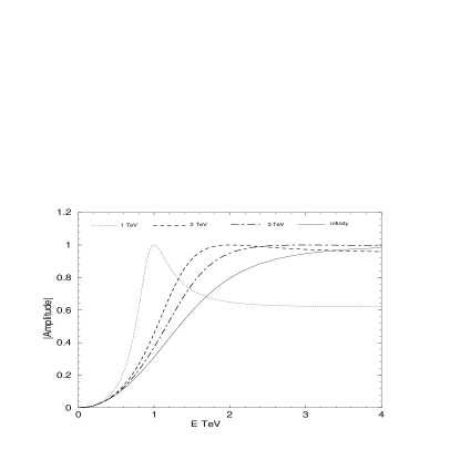
Figure 10: Comparison of absolute value of unitarized amplitude $\left|T_{0}^{0}\right|$ for $m_{\sigma b}=1(dotted),2(dashed),3(dash-dotted),\infty(solid)$ TeV.

VI Additional discussion of the electroweak model

We just discussed the $W_{L}-W_{L}$ scattering making use of the simple K-matrix unitarization and the Equivalence Theorem. This has an application to the “W-fusion” reaction shown in Fig. 5. Now we point out that a similar method can be used to take into account strong final state interactions in the “gluon-fusion” reaction GGMN78 schematically illustrated in Fig. 11. This is an interesting reaction since it is predicted GHPTW87 ; D88 ; GvdB89 ; KD91 that gluon fusion will be an important source of Higgs production. The t-quark shown running around the triangle makes the largest contribution because the quarks, of course, couple to the Higgs boson proportionally to their masses. According to the Equivalence Theorem, at high energies this Feynman diagram will contain a factor ${{g_{\sigma\pi\pi}}\over{(m_{\sigma b}^{2}-s)}}$ where the $\pi$’s correspond to the $W_{L}$’s and $g_{\sigma\pi\pi}=\frac{m_{\sigma b}^{2}}{v}$ appears in the trilinear interaction term $\frac{g_{\sigma\pi\pi}}{2}{\sigma}{\mbox{\boldmath${\pi}$}}\cdot{\mbox{\boldmath${\pi}$}}$ obtained from Eqs. (1) and (4). The need for unitarization is signaled, as in the WW scattering case by the fact that this diagram has a pole at $s=m_{\sigma b}^{2}$. Now it is necessary to regularize a three point rather than a four point amplitude; this is discussed in AS94 ; Chung . The WW scattering amplitude ${[T_{0}^{0}]}_{\rm tree}$ in the previous section was unitarized by replacing

$${[T_{0}^{0}]}_{\rm tree}\longrightarrow\frac{{[T_{0}^{0}]}_{\rm tree}}{1-i{[T_{0}^{0}]}_{\rm tree}}={[T_{0}^{0}]}_{\rm tree}\left(1+i{[T_{0}^{0}]}_{\rm tree}-{[T_{0}^{0}]}_{\rm tree}^{2}+\ldots\right).$$ (26)

Figure 11: Gluon Fusion Reaction

This has the structure of a bubble sum with the intermediate ”Goldstone bosons” on their mass shells. For the gluon fusion reaction the final ”Goldstone bosons” similarly rescatter and we should replace

$$\frac{g_{\sigma\pi\pi}}{m_{\sigma b}^{2}-s} \longrightarrow \frac{g_{\sigma\pi\pi}}{m_{\sigma b}^{2}-s}\frac{1}{1-i{[T_{0}^{0}]}_{\rm tree}}$$ (27)

$$= \frac{g_{\sigma\pi\pi}}{m_{\sigma b}^{2}-s}\cos\delta_{0}^{0}{\rm e}^{i\delta_{0}^{0}}.$$

In the second step we used the relation for the phase shift $\delta_{0}^{0}$ in the K-matrix unitarization scheme: $\tan\delta_{0}^{0}={[T_{0}^{0}]}_{\rm tree}$, where the unitarized I=J=0 S-matrix element is given by $S_{0}^{0}=\exp{2i\delta_{0}^{0}}$.

It is especially interesting to examine the quantity ${\rm\cos}\delta_{0}^{0}(s)$ which corresponds to the reduction in magnitude of the unitarized gluon fusion amplitude from the one shown in Fig. 11. Using Eq. (9) it is straightforward to find

$$\cos\delta_{0}^{0}(s)=\frac{m_{\sigma b}^{2}-s}{{[{\left(m_{\sigma b}^{2}-s\right)}^{2}+{\left(\alpha(s)\left(m_{\sigma b}^{2}-s\right)+\beta\right)}^{2}]}^{\frac{1}{2}}}.$$ (28)

The numerator cancels the pole at $s=m_{\sigma b}^{2}$ in Eq. (27) so one has the finite result:

$$[\frac{g_{\sigma\pi\pi}}{m_{\sigma b}^{2}-s}\cos\delta_{0}^{0}](s=m_{\sigma b}^{2})=\frac{32\pi v}{3m_{\sigma}b}^{2}.$$ (29)

It is clear that the factor ${\rm cos}\delta_{0}^{0}(s)$ in Eq. (27) effectively replaces the tree level denominator $(m_{\sigma b}^{2}-s)$ by the magnitude of the quantity in Eq. (17), which defines the physical pole position in the complex s plane and which we used to identify the physical Higgs mass. Note that, as in the W-fusion situation, the regularization is required for any value of $m_{\sigma b}$ (not just the large values) in order to give physical meaning to the divergent expression. The regularized electroweak factor for the amplitude of Fig. 11, $\frac{g_{\sigma\pi\pi}\cos\delta_{0}^{0}}{m_{\sigma b}^{2}-s}$, is plotted as a function of $E=\sqrt{s}$ in Fig. 12 for the cases $m_{\sigma b}=0.5,\,1.0,\,1.5,\,2.0,\,2.5,\,3.0$ TeV. It is very interesting to observe that these graphs clearly show a peaking which is correlated with the physical Higgs mass [taken, say, as $\sqrt{{\rm Re}(z_{0})}$] rather than the bare Higgs mass, $m_{\sigma b}$. At $m_{\sigma b}=0.5$ TeV one is still in the region where the physical mass is close to $m_{\sigma b}$. Already at $m_{\sigma b}=1.0$ TeV the peak has markedly broadened and is located at about 0.89 TeV. At $m_{\sigma b}=2.0$ TeV the still broader peak is located near 1.03 TeV, which is about as large as the physical mass ever gets. Beyond this, the peak continues to broaden but the location of the physical mass goes to smaller $s$. For example, at $m_{\sigma b}=3.0$ TeV, the peak is down to 0.88 TeV and is much less pronounced. Going further the curves do not look very different from the one with $m_{\sigma b}=\infty$, shown in Fig. 13. Here the peaking has disappeared and we have the analytic form (recall that $g_{\sigma\pi\pi}=\frac{m_{\sigma b}^{2}}{v}$):

$$\lim_{m_{\sigma b}\rightarrow\infty}(\frac{g_{\sigma\pi\pi}\cos\delta_{0}^{0}(s)}{m_{\sigma b}^{2}-s})={[v^{2}+{(\frac{s}{16\pi v})}^{2}]}^{-\frac{1}{2}}.$$ (30)

This is the analog of Eq. (25) and corresponds to the unitarized minimal non-linear sigma model. It still takes into account final state interaction effects in direct production of WW or ZZ pairs from gg fusion. The non-trivial structure is seen to be confined to the region $s^{1/2}$ less than about 5 TeV. There might be a sense in which such a prescription could be appropriate for a situation with an arbitrarily heavy Higgs boson BDV91 .

Figure 12: Unitarized electroweak factor $\frac{g_{\sigma\pi\pi}\cos\delta_{0}^{0}}{m_{\sigma b}^{2}-s}$, plotted as a function of $E=\sqrt{s}$ for the cases $m_{\sigma b}=0.5,\,1.0,\,1.5,\,2.0,\,2.5,\,3.0$ TeV.

Figure 13: Unitarized electroweak factor $\frac{g_{\sigma\pi\pi}\cos\delta_{0}^{0}}{m_{\sigma b}^{2}-s}$, plotted as a function of $E=\sqrt{s}$ for the cases $m_{\sigma b}=4,\infty$.

It is amusing to compare the effect of the present regularization prescription, Eq. (27) for the divergence at $s=m_{\sigma b}^{2}$ with that of the conventional Breit Wigner prescription used for example in GvdB89 ; KD91 , given in Eq. (12) with $\Gamma=\Gamma_{tree}$. These are plotted for $m_{\sigma b}=1,2,3$ TeV in Fig. 14. The main observation is that, although the absolute value of the factor in Eq. (12) flattens out due to the fact that the tree-level Higgs width (to vector bosons) increases cubically so the Higgs signal gets lost for larger $m_{\sigma b}$, the factor in Eq. (27) still has a peak at lower energies. Also the magnitude of the modified factor suggested in Eq. (27) is larger than the corresponding Breit Wigner factor. Other alternatives to the Breit-Wigner prescription for treating the divergence at $s=m_{\sigma b}^{2}$ in the gluon fusion Higgs production mechanism in Fig. 11 are momentum-dependent modifications of the Higgs width VW92 ; S95 and explicit calculation of radiative corrections GvdB96 .

Of course, the electroweak amplitude factor we have been discussing must be folded together with the triangle and gluon part of Fig. 11 as well as the gluon wavefunctions of the initiating particles. Furthermore only the I=J=0 partial wave amplitude has been considered. If various partial wave amplitudes are added, the “final state interaction” phase factor in Eq. (27), $\exp{[i\delta_{0}^{0}(s)]}$ must be included too. The value of $\delta_{0}^{0}(s)$ may be readily obtained from Eq. (28). ${\rm cos}\delta_{0}^{0}(s)$ is plotted in Fig. 15 for representative values of $m_{\sigma b}$. For a detailed practical implementation of this model it would be appropriate to take into account the relatively strong coupling of the Higgs boson to the $t{\bar{t}}$ channel. This could be conveniently accomplished by unitarizing the two channel $W_{L}W_{L}-t{\bar{t}}$ scattering matrix.

Figure 14: Comparison of modulus of unitarized electroweak factors in Higgs production amplitude: (i) $\frac{g_{\sigma\pi\pi}\cos{\delta_{0}^{0}}}{m_{\sigma b}^{2}-s}$ for the present regularization scheme (solid) and (ii) prescription of including the tree-level Higgs width (dashed) shown in Eq. (12). Here the three graphs correspond to $m_{\sigma b}=1,2,3$ TeV.

Figure 15: Plots of $cos(\delta_{0}^{0}(s))$ for $m_{\sigma b}=0.5,1.0,1.5,2.0,2.5,3.0$TeV

On noting that, as we have illustrated (see also Fig. 6), there are two bare mass values (with different widths) for each physical mass one might wonder if a very light Higgs boson could exist in the strongly interacting mode. Possibly its contribution to “precision electroweak corrections” would be comparable to those of their light bare mass images. This seems interesting, although the corresponding bare masses would be very large ($>10$ TeV according to Fig. 6), beyond where the validity of the model has been tested by the QCD analog. For bare masses in this region it would seem most reasonable to approximate the situation by using the $m_{\sigma b}\rightarrow\infty$ case.

In this paper we first noted that the K-matrix unitarized linear SU(2) sigma model could explain the experimental data in the scalar channel of QCD up to about 800 MeV. Since it is just a scaled version of the minimal electroweak Higgs sector, which is often treated with the same unitarization method, we concluded that there is support for this approach in the electroweak model up to at least Higgs bare mass about 2 TeV. We noted that the relevant QCD effective Lagrangian needed to go higher in energy is more complicated than the SU(2) linear sigma model and is better approximated by the linear SU(3) sigma model. This enabled us to extend the energy range of experimental agreement at the QCD level by including another scalar resonance. Similarly in the electroweak theory there are many candidates - e.g. larger Higgs sectors, larger gauge groups, supersymmetry, grand unified theories, technicolor, string models and recently, symmetry breaking by background chemical potentials mu - which may give rise to more than one Higgs particle in the same channel. We interpreted the better agreement at larger energies in the QCD model as also giving support to a similar treatment for a perhaps (to be seen in the future) more realistic Higgs sector in the electroweak theory which may be valid at higher energies due to additional higher mass resonances. Nevertheless we noted that even with one resonance, the minimal K matrix unitarized model behaved smoothly at large bare mass by effectively ”integrating out” the Higgs while preserving unitarity.

With added confidence in this simple approach we made a survey of the Higgs sector for the full range of bare Higgs mass. While a lot of work in this area has been done in the past we believe that some new points were added. In particular, we have noted that in this scheme the characteristic factor of the W-W fusion mechanism for Higgs production peaks at the bare mass of the Higgs boson, while the characteristic factor for the gluon fusion mechanism peaks at the generally lower physical mass.

It should be remarked that while the simplest K-matrix method of unitarization used here seems to work reasonably well, it is not at all unique. For example, Eq. (14) might be replaced by

$$S_{0}^{0}(s)=\frac{1+i({[T_{0}^{0}]}_{\rm tree}+f(s))}{1-i({[T_{0}^{0}]}_{\rm tree}+f(s))},$$ (31)

where $f(s)$ is an arbitrary real function. However the fit in Section III is good up to scaled energy, ${\bar{s}}=\frac{s}{\sqrt{2}v}\approx 6$. Thus $f(s)$ is expected to be small, at least for this energy range. A simple modification DR in this framework is to take $f(s)=$ Re$[T^{0}_{0}(s)]_{1loop}$. Of course this is not guaranteed to be more accurate at large s in the non perturbative region. Other approaches include using the large N approximation W91 , the Pade approximant method DHT90 ; DR ; W91 , the Inverse Amplitude method DHT90 ; IAM , variational approaches S01 and the N/D method O99 . It is beyond the scope of this paper to compare the different approaches.

- (1) See the dedicated conference proceedings, S. Ishida et al “Possible existence of the sigma meson and its implication to hadron physics”, KEK Proceedings 2000-4, Soryyushiron Kenkyu 102, No. 5, 2001. Additional points of view are expressed in the proceedings, D. Amelin and A.M. Zaitsev “Hadron Spectroscopy”, Ninth International Conference on Hadron Spectroscopy, Protvino, Russia(2001).
- (2) E. van Beveren, T.A. Rijken, K. Metzger, C. Dullemond, G. Rupp and J.E. Ribeiro, Z. Phys. C30, 615 (1986). E. van Beveren and G. Rupp, hep-ph/9806246, 248. See also J.J. de Swart, P.M.M. Maessen and T.A. Rijken, U.S./Japan Seminar on the YN Interaction, Maui, 1993 [Nijmegen report THEF-NYM 9403].
- (3) D. Morgan and M. Pennington, Phys. Rev. D48, 1185 (1993).
- (4) A.A. Bolokhov, A.N. Manashov, M.V. Polyakov and V.V. Vereshagin, Phys. Rev. D48, 3090 (1993). See also V.A. Andrianov and A.N. Manashov, Mod. Phys. Lett. A8, 2199 (1993). Extension of this string-like approach to the case has been made in V.V. Vereshagin, Phys. Rev. D55, 5349 (1997) and in A.V. Vereshagin and V.V. Vereshagin, ibid. 59, 016002 (1999).
- (5) N.N. Achasov and G.N. Shestakov, Phys. Rev. D49, 5779 (1994).
- (6) R. Kamínski, L. Leśniak and J. P. Maillet, Phys. Rev. D50, 3145 (1994).
- (7) F. Sannino and J. Schechter, Phys. Rev. D52, 96 (1995).
- (8) N.A. Törnqvist, Z. Phys. C68, 647 (1995) and references therein. In addition see N.A. Törnqvist and M. Roos, Phys. Rev. Lett. 76, 1575 (1996), N.A. Törnqvist, hep-ph/9711483 and Phys. Lett. B426 105 (1998).
- (9) R. Delbourgo and M.D. Scadron, Mod. Phys. Lett. A10, 251 (1995). See also D. Atkinson, M. Harada and A.I. Sanda, Phys. Rev. D46, 3884 (1992).
- (10) G. Janssen, B.C. Pearce, K. Holinde and J. Speth, Phys. Rev. D52, 2690 (1995).
- (11) M. Svec, Phys. Rev. D53, 2343 (1996).
- (12) S. Ishida, M.Y. Ishida, H. Takahashi, T. Ishida, K. Takamatsu and T Tsuru, Prog. Theor. Phys. 95, 745 (1996), S. Ishida, M. Ishida, T. Ishida, K. Takamatsu and T. Tsuru, Prog. Theor. Phys. 98, 621 (1997). See also M. Ishida and S. Ishida, Talk given at 7th International Conference on Hadron Spectroscopy (Hadron 97), Upton, NY, 25-30 Aug. 1997, hep-ph/9712231.
- (13) M. Harada, F. Sannino and J. Schechter, Phys. Rev. D54, 1991 (1996).
- (14) M. Harada, F. Sannino and J. Schechter, Phys. Rev. Lett. 78, 1603 (1997).
- (15) D. Black, A.H. Fariborz, F. Sannino and J. Schechter, Phys. Rev. D58, 054012 (1998).
- (16) D. Black, A.H. Fariborz, F. Sannino and J. Schechter, Phys. Rev. D59, 074026 (1999).
- (17) J.A. Oller, E. Oset and J.R. Pelaez, Phys. Rev. Lett. 80, 3452 (1998). See also K. Igi and K. Hikasa, Phys. Rev. D59, 034005 (1999).
- (18) A.V. Anisovich and A.V. Sarantsev, Phys. Lett. B413, 137 (1997).
- (19) V. Elias, A.H. Fariborz, Fang Shi and T.G. Steele, Nucl. Phys. A633, 279 (1998).
- (20) V. Dmitrasinović, Phys. Rev. C53, 1383 (1996).
- (21) P. Minkowski and W. Ochs, Eur. Phys. J. C9, 283 (1999).
- (22) S. Godfrey and J. Napolitano, hep-ph/9811410.
- (23) L. Burakovsky and T. Goldman, Phys. Rev. D57 2879 (1998)
- (24) A. H. Fariborz and J. Schechter, Phys. Rev D60, 034002 (1999).
- (25) D. Black, A. H. Fariborz and J. Schechter, Phys. Rev. D61 074030 (2000). See also V. Bernard, N. Kaiser and U-G. Meissner, Phys. Rev. D 44, 3698 (1991).
- (26) D. Black, A. H. Fariborz and J. Schechter, Phys. Rev. D61 074001 (2000).
- (27) L. Celenza, S-f Gao, B. Huang and C.M. Shakin, Phys. Rev. C 61, 035201 (2000).
- (28) D. Black, A.H. Fariborz, S. Moussa, S. Nasri and J. Schechter, Phys.Rev. D64, 014031 (2001).
- (29) R. L. Jaffe, Phys. Rev. D15, 367 (1977).
- (30) In addition to BFS3 and BFMNS01 above see T. Teshima, I. Kitamura and N. Morisita, J. Phys. G. 28, L391 (2002); F. Close and N. Tornqvist, ibid. 28, R249 (2002) and A. H. Fariborz, hep-ph/0302133.
- (31) See section V of BFMNS01 above.
- (32) M. Gell-Mann and M. Lévy, Nuovo Cimento 16, 705 (1960).
- (33) In addition to GL above see J. Cronin, Phys. Rev. 161, 1483 (1967); S. Weinberg, Phys. Rev. Lett 18, 188 (1967).
- (34) J. Gasser and H. Leutwyler, Ann. Phy. 158, 142 (1984).
- (35) A. Abdel-Rehim, D. Black, A. H. Fariborz and J. Schechter, hep-ph/0304177.
- (36) J.M. Cornwall, D.N. Levin and G. Tiktopoulos, Phys. Rev. D10, 1145 (1974).
- (37) B.W. Lee, C. Quigg and H.B. Thacker, Phys. Rev. D16 1519 (1977).
- (38) M.S. Chanowitz and M.K. Gaillard, Nucl. Phys. B261 (1985) 379.
- (39) J. Bagger and C. Schmidt, Phys. Rev. D 41, 264 (1990).
- (40) S.De Curtis, D. Dominici and J.R. Pelaez, hep-ph/0211353.
- (41) W. W. Repko and C. S. Suchyta, III, Phys. Rev. Lett. 62, 859 (1989).
- (42) D. A. Dicus and W. W. Repko Phys. Lett. B 228, 503 (1989); Phys. Rev. D42, 3660 (1990).
- (43) S. Willenbrock, Phys. Rev. D43 1710 (1991).
- (44) M. S. Chanowitz, Phys. Rev. D66 073002 (2002) and hep-ph/0304199.
- (45) The LEP Collaborations, the LEP Electroweak Working Group and the SLD Heavy Flavor and Electroweak Groups, hep-ex/0212036.
- (46) G. P. Zeller et al, Phys. Rev. Lett. 88, 091802 (2002).
- (47) W. Loinaz, N. Okamura, T. Takeuchi and L. C. R. Wijewardhana, Phys. Rev. D67 073012 (2003).
- (48) For a discussion of how gauge boson scattering may be incorporated into the annihilation cross section see for example pages 197-199 of Effective Lagrangians for the Standard Model, A. Dobado, A. Gómez-Nicola, A.L. Maroto and J.R. Peláez, Springer-Verlag Berlin Heidelberg 1997.
- (49) H.M. Georgi, S.L. Glashow, M.E. Machacek and D.V. Nanopoulos, Phys. Rev. Lett. 40, 692 (1978).
- (50) S. U. Chung et al, Ann. Physik 4 404 (1995).
- (51) E.A. Alekseeva et al., Sov. Phys. JETP 55, 591 (1982), G. Grayer et al., Nucl. Phys. B75, 189 (1974).
- (52) M. Lévy, Nuovo Cimento 52A, 23 (1967). See S. Gasiorowicz and D. A. Geffen, Rev. Mod. Phys. 41, 531 (1969) for a review which contains a large bibliography.
- (53) J. Schechter and Y. Ueda, Phys. Rev. D3, 2874, 1971; Erratum D 8 987 (1973). See also J. Schechter and Y. Ueda, Phys. Rev. D3, 168, (1971).
- (54) J. Schechter and Y. Ueda, Phys. Rev. D 4, 733 (1971).
- (55) See also L.H. Chan and R. W. Haymaker, Phys. Rev. 07, 402 (1973); 10, 4170 (1974).
- (56) J. Donoghue, C. Ramirez and G. Valencia, Phys.Rev. D39 , 1947 (1989); G. Ecker, J. Gasser, A. Pich and E. de Rafael, Nucl. Phys. B321, 311 (1989); G. Ecker, J. Gasser, H. Leutwyler, A. Pich and E. de Rafael, Phys. Lett. B233, 425 (1989).
- (57) W. Hudnall, Phys. Rev. D6, 1953 (1972).
- (58) For the Standard Model case it has been explicitly verified that the one-loop corrections to the J=0 WW/ZZ scattering amplitude, discussed in Section V, become large for TeV. See S. Dawson and S. Willenbrock, Phys. Rev. Lett. 62 1232, 1989.
- (59) In the case where the pion mass is retained in Eqs. (10), behaves identically as in the case while the “physical” sigma mass, , approaches the small constant value 0.22 GeV. The “physical” sigma width, approaches the relatively large constant value 1.96 GeV. Qualitatively, this is in agreement with the case.
- (60) A. Dobado and M.J. Herrero, Phys. Lett B228 495 (1989).
- (61) J.F. Donoghue and C. Ramirez, Phys. Lett. B234, 361 (1990).
- (62) This best fit value of was found when the physical pion mass is taken. As discussed in Section IV, the QCD results do not change too much if we set .
- (63) The fact that can be understood as due to the opposite signs of and in Eq. (9). This is explained in more detail in the next-to-last paragraph of Section III in BFMNS01 .
- (64) R. Casalbuoni, D. Dominici and R. Gatto, Phys. Lett. B 147, 419 (1984).
- (65) J. Pasupathy, Mod. Phys. Lett. A12, 1605 (2000).
- (66) J.F. Gunion, H.E. Haber, F.E. Paige, Wu-Ki Tung and S.S.D. Willenbrock, Nucl. Phys. B294, 621 (1987).
- (67) D.A. Dicus, Phys. Rev. D 38, 394 (1988).
- (68) E.W.N. Glover and J.J. van der Bij, Phys. Lett B219 488 (1989). E.W.N. Glover and J.J. van der Bij, Nucl. Phys. B321 (1989) 561.
- (69) C. Kao and D.A. Dicus, Phys. Rev. D43 1555 (1991).
- (70) The one-loop result for this case is given in J. Bagger, S. Dawson and G. Valencia, Phys. Rev. Lett. 67, 2256 (1991).
- (71) G. Valencia and S. Willenbrock, Phys. Rev. D 46, 2247 (1992).
- (72) M.H. Seymour, Phys. Lett B 354 (1995) 409.
- (73) A. Ghinculov and J.J. van der Bij, Nucl. Phys. B 482 59 (1996).
- (74) F. Sannino and K. Tuominen, hep-ph/0303167.
- (75) A. Dobado, M.J. Herrero and T.N. Truong, Phys. Lett. B 235, 129 (1990), ibid B235, 134 (1990). A. Dobado ibid B 237, 457 (1990). A. Dobado, M.J. Herrero and J. Terron, Zeit. Phys. C50, 205 (1991) and 465 (1991).
- (76) J.R. Peláez, Phys. Rev. D55 4193 (1997).
- (77) F. Siringo, Europhys. Lett. 57 (2002) 820 - 826.
- (78) J.A. Oller, Phys. Lett. B477 (2000) 187-194.