IMSc-2003/05/09
Mesons: Relativistic Bound States with String Tension

Abstract

A systematic method of analysing Bethe-Salpeter equation using spectral representation for the relativistic bound state wave function is given. This has been explicitly applied in the context of perturbative QCD with string tension in the $1\over N$ expansion. We show that there are only a few stable bound state mesons due to the small ”threshold mass”(constituent mass) of quarks. The asymptotic properties of the bound states are analytically analysed. The spectrum is derived analytically and compared phenomenologically. Chiral symmetry breaking and PCAC results are demonstrated. We make a simple minded observation to determine the size of the bound states as a function of the energy of the boundstate.

Keywords: QCD, Mesons, String Tension, Bethe-Salpeter Equation, PCAC.

1 Introduction

We address relativistic bound states which are due to a causal interaction kernel. Investigation of these systems is essential to understand approximate Goldstones such as the physical pion. Wick-Cutkosky(WC) model[1, 2] was one such model which was investigated in great detail, wherein they have presented a fairly general series expansion technique. Here we simplify and make their formalism more transparent and infact we find that “deeply bound states”, those whose binding energy is comparable or more than the rest mass energy due to a very strong interaction kernel can be understood in a simpler way. An important observation has been that the most general “spectral” representation [3] for the bound state wave function exists and is very simple to work with. WC wave functions are a special class of this representation.

In this work we will study quark-antiquark($\bar{q}q$) bound states in the Bethe-Salpeter(BS) formalism in the context of the field theoretic model ($\sigma QCD$) proposed in [4]. To recapitulate the essential points of this model, string tension term($\frac{\sigma}{k^{4}}$) was explicitly incorporated in perturbative QCD using auxillary fields such that ultraviolet renormalisation is assured. The ultraviolet(UV) behaviour remains the same as in QCD. The string tension($\sigma$) vanishes asymptotically in the UV limit. In this model we will be working in the leading $\frac{1}{N}$ approximation and $g^{2}N$ is assumed to be small for all energies where $g$ is the QCD gauge coupling constant. The infrared singular confining part of the interaction is given by the string tension term. Our analysis is done in Minkowski(+,-,-,-) space.

In $\sigma QCD$ with our approximations we have seen that the quark propagator has no pole and it does not have a simple pole structure[5] unlike in WC model. Consequently the BS equation which involves the quark propagator has more algebraic complications. Even then the bound state spectral representation is still valid and this enables us to perform analytic calculations. Qualitatively we see that quark propagator poles are missing but they have “threshold masses”[5] which determines the onset of the imaginary part of the propagator. This is a more precise notion in our model corresponding to constituent mass of strong interaction phenomenology. For completeness we have presented the angular decomposition of the wave function in detail. For brevity we have looked at single quark flavour system. Our analysis can equally well handle cases of more than one flavour.

In the BS bound state description of mesons we show that even in the presence of string tension there are only a few number of stable mesons and this is a consequence of the existence of the the threshold mass. There however are many unstable(complex energy) bound states and we have not made any attempt to study them systematically.

Heavy quark bound systems under certain standard assumptions do reduce to non-relativistic Schrodinger theory bound systems. This is alluded to briefly as it is well understood in the literature. As for light mesons we derive the relationship between the mass of the pion and the current quark masses consistent with PCAC.

2 Bethe-Salpeter equation

We address the quark-antiquark bound state problem in perturbative QCD with string tension. As discussed in [4, 5] there are three parameters in the theory, $\sigma N$, $g^{2}N$ and $1/N$ of which we will treat $\sigma N$ as a non-perturbative parameter and the latter two perturbatively. The BS equation (Fig[1]) for the quark-antiquark bound state in the $1/N$ expansion sums only the ladder graphs of ’$\sigma$ exchange’ (eq.(1)) where quark antiquark propagators are the non-perturbative propagators obtained by summing the rainbow ’$\sigma$ exchange’ [5].

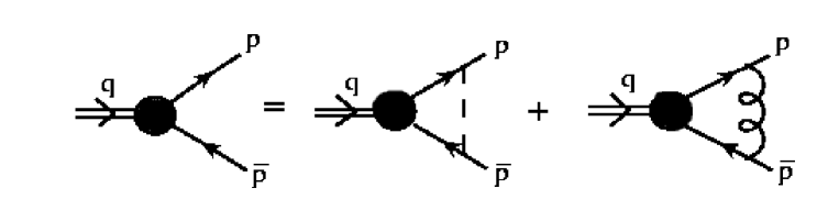
Figure 1: Bethe-Salpeter equation summing up ladder graphs.

$$\phi(p,\bar{p})=S(\bar{p})\gamma_{\mu}\int\frac{d^{4}k}{i(2\pi)^{4}}(\frac{\sigma N\phi((p-k),(\bar{p}+k))}{(p-k)^{4}}-\frac{g^{2}N\phi((p-k),(\bar{p}+k))}{(p-k)^{2}})\gamma^{\mu}S(p)$$ (1)

where $S(p)$ and $S(\bar{p})$ are the quark propagators, $\sigma$ is the string tension, $g$ is the gluon-fermion coupling constant and $N$ is the number of colours. In the above we have also included an additional $g^{2}N$ term for the following reason. It is evident in the theory that the leading UV behaviour is governed by $g^{2}$. Hence to discuss the bound state UV behaviour we need to consider this contribution too. With our ansatz of $g^{2}N$ small, we only include the leading UV behaviour (There are additional $g^{2}N$ terms interfering with $\sigma$ exchange but these are subleading in the UV regime). In this work we do not consider a running $g$ or $\sigma$.

The BS amplitude is decomposed in terms of $4\times 4$ Dirac matrices [6, 7]

$$\phi=\phi_{S}+\gamma_{5}\phi_{P}+\gamma_{\mu}\phi^{\mu}_{V}+\gamma_{\mu}\gamma_{5}\phi^{\mu}_{A}+\sigma_{\mu\nu}\phi^{\mu\nu}_{T}$$ (2)

Substituting eq.(2) in the BS equation , we get the following decomposition for the scalar, pseudoscalar, vector and pseudovector amplitudes with the propagators given by $S(p)=i(\not pA(p^{2})+B(p^{2}))$, $S(\bar{p})=i(\not\bar{p}\bar{A}(\bar{p}^{2})+\bar{B}(\bar{p}^{2}))$

$$\phi_{S}=4(\bar{A}A\bar{p}\cdot p+\bar{B}B)\int\phi_{S}-2(\bar{A}B\bar{p}_{\mu}+A\bar{B}p_{\mu})\int\phi^{\mu}_{V}$$ (3)

$$\gamma_{\mu}\phi^{\mu}_{V} = 4(A\bar{B}\not p+\bar{A}B\not\bar{p})\int\phi_{S}+2i\bar{A}A\epsilon^{\alpha\mu\beta\delta}\bar{p}_{\alpha}p_{\beta}\gamma_{\delta}\int\phi_{A\mu}$$

$$- 2(\bar{A}A(\bar{p}_{\mu}\not p-\bar{p}\cdot p\gamma_{\mu}+\bar{\not}pp_{\mu})+\bar{B}B\gamma_{\mu})\int\phi^{\mu}_{V}$$

$$\gamma_{5}\phi_{P} = 4(\bar{A}A\bar{p}\cdot p-\bar{B}B)\gamma_{5}\int\phi_{P}-2(\bar{A}B\bar{p}_{\mu}-A\bar{B}p_{\mu})\gamma_{5}\int\phi^{\mu}_{A}$$ (5)

$$\gamma_{\mu}\gamma_{5}\phi^{\mu}_{A} = 4(\bar{A}B\not\bar{p}-A\bar{B}\not p)\gamma_{5}\int\phi_{P}+2i\bar{A}A\epsilon^{\alpha\mu\beta\delta}\bar{p}_{\alpha}p_{\beta}\gamma_{\delta}\gamma_{5}\int\phi_{V\mu}$$

$$- 2(\bar{A}A(\bar{p}_{\mu}\not p-\bar{p}\cdot p\gamma_{\mu}+\bar{\not}pp_{\mu})-\bar{B}B\gamma_{\mu})\gamma_{5}\int\phi^{\mu}_{A}$$

The symbol $\int$ stands for the 4-d momentum integral corresponding to the sum of the confining and the gluon interactions.

$$\int\phi=\int\frac{i~{}d^{4}k}{(2\pi)^{4}}(\frac{\sigma N\phi((p-k),(\bar{p}+k))}{(p-k)^{4}}-\frac{g^{2}N\phi((p-k),(\bar{p}+k))}{(p-k)^{2}})$$ (7)

In addition the tensor components are totally determined by the above components.

Since the momentum of the bound states has to be time like, we can go to the centre of mass frame of the bound state wherein the total momentum vector is given by $q=(q_{0}=M,0,0,0)$ where $M$ is the mass of the bound state. The little group is $SO(3)$. In this frame the angular momentum decomposition of the BS amplitude can be done in terms of 3-d solid harmonics and $O(3)$ scalar functions of $p^{0},\vec{p}$ in the following manner,

$$\phi_{i}^{(j)}=\Phi_{i}^{(j)}(p^{0},\vec{p})y_{jm}$$ (8)

for $i=S,P,0V,0A$ $i.e.,$ Scalar ,Pseudoscalar, time component of Vector and Pseudovector respectively. The remaining $3-d$ vector components are decomposed as [8]

$$\vec{\phi}^{(j)}_{V} = (\vec{p}\Phi_{1V}^{(j)}+\vec{J}\Phi_{2V}^{(j)}+i(\vec{p}\times\vec{J})\Phi_{3V}^{(j)})y_{jm}$$

$$= \Sigma_{jm\delta}\Phi^{jm(\delta)}_{V}\vec{Y}^{(j+\delta,1)jm}(\vec{p})$$

$$\vec{\phi}^{(j)}_{A} = (\vec{p}\Phi_{1A}^{(j)}\vec{p}+\vec{J}\Phi_{2A}^{(j)}+i(\vec{p}\times\vec{J})\Phi_{3A}^{(j)})y_{jm}$$

$$= \Sigma_{jm\delta}\Phi^{jm(\delta)}_{A}\vec{Y}^{(j+\delta,1)jm}(\vec{p})$$

where $\delta=0,1$, $\phi^{\mu}_{V}=(\phi_{0V},\vec{\phi}_{V})$ , $\phi^{\mu}_{A}=(\phi_{0A},\vec{\phi_{A}})$, $y_{jm}=|\vec{p}|^{j}Y_{jm}$,where $y_{jm}$ are the solid harmonics, $\vec{J}=\vec{p}\times\vec{\nabla_{\vec{p}}}$ and $\vec{Y}^{(j+\delta,1)jm}(\vec{p})$ are the 3-d vector spherical harmonics([8]).

The relation between $\Phi_{iV}^{(j)}$ and $\Phi^{jm(\delta)}_{V}$ is given by [8]

$$\Phi_{1V}^{(j)} = -\sqrt{\frac{j+1}{2j+1}}\Phi^{jm(1)}_{V}+\sqrt{\frac{j}{2j+1}}\Phi^{jm(-1)}_{V}$$ (11)

$$\Phi_{2V}^{(j)} = \sqrt{\frac{1}{j(j+1)}}\Phi^{jm(0)}_{V}$$ (12)

$$\Phi_{3V}^{(j)} = -\sqrt{\frac{1}{(j+1)(2j+1)}}\Phi^{jm(1)}_{V}-\frac{1}{\vec{p}^{2}}\sqrt{\frac{1}{j(2j+1)}}\Phi^{jm(-1)}_{V}$$ (13)

similar equations apply for the Pseudovector part.

3 Representation of the Wave functions

In eq.(8)-eq.(LABEL:repvec) we have introduced functions of $p^{0}$ and $\vec{p}$. They are Lorentz scalars as they are defined in the rest frame of the bound state. A convenient representation is required to make our analysis transparent. Consider a scalar 3-point function. In general this is a scalar function of momenta associated with three independent Lorentz scalar quantities, namely $p^{2}$,$\bar{p}^{2}$,$q^{2}$ with $p_{\mu}-\bar{p}_{\mu}=q_{\mu}$ owing to momentum conservation. Any scalar function associated with the 3-point function is a function of these three variables. There exists a spectral representation for such a function, that of Deser,$et.al,$ [9]. In the BS wave function we are in a similar situation with one of the scalar variables namely $q^{2}$ fixed due to an eigenvalue condition. There are many equivalent ways of representing such a spectral representation. We find the most convenient one is due to [3],

$$\phi(\bar{p}^{2},p^{2}) = \int_{0}^{1}dy\int_{\delta^{2}}^{\infty}d\alpha\frac{\tilde{\phi}(\alpha,y)}{(p-yq)^{2}-\alpha+i\epsilon}$$

$$= \int_{0}^{1}dy\tilde{\Phi}((p-yq)^{2},y)$$

Note that $(p-yq)^{2}=(1-y)p^{2}+y\bar{p}^{2}-y(1-y)q^{2}$.

The spectral function $\tilde{\phi}(\alpha,y)$ in general is complex and range of $\alpha$ can be from zero to infinity. For a stable bound state we know from physical considerations that it has a finite size and for certain range of energies of the constituents this size is not infinity. The size of the bound state is defined by the onset of exponential fall off in co-ordinate space. This is possible only if the $\alpha$ integration range is above some positive nonvanishing quantity $\delta^{2}$ where $\delta$ is the inverse of the size of the bound state. In general $\delta$ many depend on $y$. Here we will take it to be the minimum possible value in the range of integration. In WC model[2] the BS wavefunction can be cast into the above form where $\delta^{2}(y)$ is fixed in terms of masses of the constituents and $\tilde{\phi}$ is a series in derivatives of $\delta(\alpha-\delta^{2})$. This is also a simple case of the so called Perturbation Theory Integral representation [10]. Substituting this representation for the each of the scalar functions eq.(8), we can do the loop momentum integrals by introducing the appropriate Feynman parameter integrals as shown in detail in [5]. It is instructive to note the following self-reproducing property of the solid harmonics which follows from the defining property [2], namely, $\nabla_{\vec{p}}^{2}y_{jm}(\vec{p})=0$

$$\int d^{3}kF(\vec{k}^{2})y_{jm}(\vec{k}+\vec{p})=y_{jm}(\vec{p})\int d^{3}kF(\vec{k}^{2})$$ (15)

where $F(\vec{k}^{2})$ is a sufficiently well behaved function.

[S][V] SECTOR:

$$\int\tilde{\Phi}_{S}^{(j)} = 4(\bar{A}A\bar{p}\cdot p+\bar{B}B)\int\int\tilde{\Phi}_{S}^{(j)}-2(\bar{A}B\bar{p}^{0}+A\bar{B}p^{0})\int\int\tilde{\Phi}_{0V}^{(j)}$$

$$+ 2(\bar{A}B+A\bar{B})\vec{p}^{2}\int\int\tilde{\Phi}_{1V}^{(j)}$$

$$\int\tilde{\Phi}_{0V}^{(j)} = 4(\bar{A}B\bar{p}^{0}+A\bar{B}p^{0})\int\int\tilde{\Phi}_{S}^{(j)}+2(\bar{A}A\bar{p}\cdot p-\bar{B}B-\bar{A}A\bar{p}^{0}p^{0})\int\int\tilde{\Phi}_{0V}^{(j)}$$

$$+ 2\bar{A}A(\bar{p}^{0}+p^{0})\vec{p}^{2}\int\int\tilde{\Phi}_{1V}^{(j)}$$

$$\int\tilde{\Phi}_{1V}^{(j)} = 4(\bar{A}B+A\bar{B})\int\int\tilde{\Phi}_{S}^{(j)}-2\bar{A}A(\bar{p}^{0}+p^{0})\int\int\tilde{\Phi_{0V}^{(j)}}$$

$$+ 2(\bar{A}A\bar{p}\cdot p-\bar{B}B+2\bar{A}A\vec{p}^{2})\int\int\tilde{\Phi}_{1V}^{(j)}$$

[P][A]-SECTOR:

$$\int\tilde{\Phi}_{P}^{(j)} = 4(\bar{A}A\bar{p}\cdot p-\bar{B}B)\int\int\tilde{\Phi}_{P}^{(j)}-2(\bar{A}B\bar{p}^{0}-A\bar{B}p^{0})\int\int\tilde{\Phi}_{0A}^{(j)}$$

$$+ 2(\bar{A}B-A\bar{B})\vec{p}^{2}\int\int\tilde{\Phi_{1A}^{(j)}}$$

$$\int\tilde{\Phi}_{0A}^{(j)} = 4(\bar{A}B\bar{p}^{0}-A\bar{B}p^{0})\int\int\tilde{\Phi}_{P}^{(j)}+2(\bar{A}A\bar{p}\cdot p+\bar{B}B-2\bar{A}A\bar{p}^{0}p^{0})\int\int\tilde{\Phi}_{0A}^{(j)}$$

$$+ 2\bar{A}A(\bar{p}^{0}+p^{0})\vec{p}^{2}\int\int\tilde{\Phi}_{1A}^{(j)}$$

$$\int\tilde{\Phi}_{1A}^{(j)} = 4(\bar{A}B-A\bar{B})\int\int\tilde{\Phi}_{P}^{(j)}-2\bar{A}A(\bar{p}^{0}+p^{0})\int\int\tilde{\Phi}_{0A}^{(j)}$$

$$+ 2(\bar{A}A\bar{p}\cdot p+\bar{B}B+2\bar{A}A\vec{p}^{2})\int\int\tilde{\Phi}_{1A}^{(j)}$$

THE [V][A] Mixed Sector: for j$\geq$1

$$\int\tilde{\Phi}_{2A}^{(j)} = 2(\bar{A}A\bar{p}\cdot p+\bar{B}B)\int\int\tilde{\Phi}_{2A}^{(j)}+2\bar{A}Aq^{0}\vec{p}^{2}\int\int\tilde{\Phi}_{3V}^{(j)}$$ (22)

$$\int\tilde{\Phi}_{3V}^{(j)} = 2(\bar{A}A\bar{p}\cdot p-\bar{B}B)\int\int\tilde{\Phi}_{3V}^{(j)}+2\bar{A}Aq^{0}\int\int\tilde{\Phi}_{2A}^{(j)}$$ (23)

$$\int\tilde{\Phi}_{2V}^{(j)} = 2(\bar{A}A\bar{p}\cdot p-\bar{B}B)\int\int\tilde{\Phi}_{2V}^{(j)}+2\bar{A}Aq^{0}\vec{p}^{2}\int\int\tilde{\Phi}_{3A}^{(j)}$$ (24)

$$\int\tilde{\Phi}_{3A}^{(j)} = 2(\bar{A}A\bar{p}\cdot p+\bar{B}B)\int\int\tilde{\Phi}_{3A}^{(j)}+2\bar{A}Aq^{0}\int\int\tilde{\Phi}_{2V}^{(j)}$$ (25)

Where the symbol $\int$ stands for

$$\int\tilde{\Phi}_{i}^{(j)}=\int_{0}^{1}dy\tilde{\Phi}_{i}^{(j)}((p-yq)^{2},y))$$

and $\int\int$ stands for

$$\int\int\tilde{\Phi}_{i}^{(j)} = \frac{\sigma N}{(4\pi)^{2}}\int_{0}^{1}dx\int_{0}^{1}\frac{dy}{1-x}(x^{j+1}\tilde{\Phi}_{i}^{(j)}(x(p-yq)^{2},y)-\tilde{\Phi}_{i}^{(j)}((p-yq)^{2},y))$$

$$+ \frac{g^{2}N}{(4\pi)^{2}}\int_{0}^{1}dx\int_{0}^{1}dy\int_{-\infty}^{x(p-yq)^{2}}d\beta x^{j}\tilde{\Phi}_{i}^{(j)}(\beta,y)$$

for $i=S,P,0V,0A,2V,2A$. The $x^{j}$ in the previous equation is replaced by $x^{j+1}$ for $i=1V,3V,1A,3A$ and the equations are written in units of $\frac{\sigma N}{(4\pi)^{2}}=\bar{\sigma}=1$. Also we define $\frac{g^{2}N}{(4\pi)^{2}}=\bar{\alpha}$.

These coupled integral equations essentially become four different cases as expected from angular momentum algebra, namely the sum of two spin $1/2$ and orbital angular momentum $l$, yields total angular momentum $j$ as

$$j=l\otimes\frac{1}{2}\otimes\frac{1}{2}=l\otimes(0\oplus 1)=l\oplus l-1\oplus l\oplus l+1$$ (27)

This explicit decomposition manifested in eq.(3)-(25) is as far as we know a new result.

4 Asymptotic Behaviour

First we consider the behaviour of the wave function for large space like $p^{2}$. Here the wave function is real and probes the short distance behaviour. The integral equation does not couple the UV behaviour of the wave function to the IR or intermediate regime of the theory. The UV behaviour of the wavefunction is determined self-consistently by the UV interaction alone. The leading UV behaviour of $\sigma QCD$ is the same as in QCD. Using the asymptotic behaviour of $A(p^{2})$ and $B(p^{2})$,

$$A(p^{2}) \sim -\frac{1}{-p^{2}\sqrt{2\bar{\alpha}\ln(-p^{2})}}$$ (28)

$$B(p^{2}) \sim \frac{\ln(-p^{2})}{-p^{2}}$$ (29)

we adopt the same procedure as shown in [5].

The leading order asymptotic behaviour of the BS amplitudes in the [P][A] and [S][V] sector are the same. Its in the next to leading order(NLO) that they differ. The leading order BS amplitudes go like,

$$\phi_{P}^{(j)} \sim \phi_{S}^{(j)}\sim\frac{1}{(-p^{2})^{j+2}(\ln(-p^{2}))^{1+\frac{2}{j+1}}}$$ (30)

$$\phi_{0A}^{(j)} \sim \phi_{0V}^{(j)}\sim\frac{1}{(-p^{2})^{j+2}(\ln(-p^{2}))^{1+\frac{1}{j+1}}}$$ (31)

$$\phi_{1A}^{(j)} \sim \phi_{1V}^{(j)}\sim\frac{1}{(-p^{2})^{j+3}(\ln(-p^{2}))^{1-\frac{1}{j+2}}}$$ (32)

For $j\geq 1$

$$\phi_{2V}^{(j)} \sim \phi_{2A}^{(j)}\sim\frac{1}{(-p^{2})^{j+2}(\ln(-p^{2}))^{1+\frac{1}{j+1}}}$$ (33)

$$\phi_{3V}^{(j)} \sim \phi_{3A}^{(j)}\sim\frac{1}{(-p^{2})^{j+3}(\ln(-p^{2}))^{1+\frac{1}{j+2}}}$$ (34)

We have not used running $\bar{\alpha}$ in the above analysis. It is seen that $A(p^{2})$ function dominates as expected and the asymptotic behaviour of the wave function is independent of $\bar{\alpha}$ due to the dependence of $A(p^{2})$ on $\bar{\alpha}$ as given in eq.(28). It is also evident that no further infinite renormalisations are needed as the BS wavefunction asymptotic behaviour is sufficiently small that all momentum integrals are finite. This demonstrates that the theory is made finite by the standard wavefunction, mass and string tension renormalisations alone. The leading aysmptotic behaviour as shown in eq.(30)-(34) is the same both in $QCD$ and $\sigma QCD$. For completeness we mention that if we ignore the $g^{2}N$ term in eq.(1) then the asymptotic analysis, yields similar results as eq.(30)-(34) with the powers of $p^{2}$ decreased by one and all $\ln(-p^{2})$ powers are zero.

5 Spectrum of Light Mesons

The BS equation is simplified considerably in their algebraic complexity. Generically it is very much like in the WC model. Major difference being that the propagator functions are complicated functions unlike simple poles in the WC model. The eigenvalue problem is well defined once the explicit $A(p^{2})$ and $B(p^{2})$ functions of the quark propagator are given.

The most important properties of $A(p^{2})$ and $B(p^{2})$ that we exploit is that they are analytic functions near $p^{2}=0$ and the onset of non-analyticity is near the threshold mass $\tilde{m}$, $i.e.,$ $p^{2}=\tilde{m}^{2}$ in units of $\bar{\sigma}$. Considering the BS wavefunctions (3)-(25) we first note that these functions are real and analytic for $p^{2}<\tilde{m}^{2}$ and $\bar{p}^{2}<\tilde{\bar{m}}^{2}$. This is equivalent to saying that for all eigenvalues $q$ such that $q_{0}<\tilde{m}+\tilde{\bar{m}}$ the wave functions are real and analytic. It is also evident from the standard arguments [1, 2, 3] that for $q_{0}>\tilde{m}+\tilde{\bar{m}}$ the wavefunctions are necessarily complex and perhaps even unstable, $i.e.,$ the eigenvalue $q_{0}$ itself may be complex.

For light quarks where the renormalised mass(current mass) $m$ is much smaller than $\bar{\sigma}$, we have shown [5] that threshold mass(constituent mas) $\tilde{m}^{2}\ll\bar{\sigma}$, indeed we estimated that $\tilde{m}^{2}\approx.02\bar{\sigma}$. For stable mesons $q_{0}<\tilde{m}+\tilde{\bar{m}}$, consequently $q_{0}\ll\sqrt{\bar{\sigma}}$. Therefore all stable bound states in this system are necessarily deeply bound. For simplicity we ignore the gluon coupling and keep only the string tension contribution to the BS equation. We solve the BS equation at $p^{2}=\bar{p}^{2}=0$ where we know explicitly the propagator functions. Consider the case when the BS wavefunction is non vanishing at $p^{2}=\bar{p}^{2}=0$, since $q^{2}\ll 1$, we negelect the $xq^{2}$ dependence in the $r.h.s$ of eq.(3)-(25). Then all $x$ integrations can be done explicitly (The $y$ integration can be done formally on both sides). Consequently the BS equation reduces to an ordinary matrix eigenvalue equation in each of the different sectors at $p^{2}=\bar{p}^{2}=0$. Solution to these homogenous equations is guaranteed if the corresponding determinant of the matrix is zero. Noting that all our calculations are valid only if $q^{2}>0$ the relevant solutions resulting from the vanishing of the determinant are given below. The explicit answers are given for renormalised quark mass, $m=\bar{m}$.

$$\mbox{[S][V]~{} SECTOR}:~{}~{}~{}q^{2}=\frac{(2b_{0}^{2}H+1)(4b_{0}^{2}L-1)}{2a_{0}^{2}L(1-2b_{0}^{2}H)}$$ (35)

For small quark masses $m$ we have for $j=0$ and $1$, $M^{2}(j^{P})$ where $P$ is the intrinsic parity.

$$M^{2}(0^{+}) \approx \frac{1}{7}+\frac{153}{196}m$$ (36)

$$M^{2}(1^{-}) \approx \frac{5}{138}+\frac{2171}{6348}m$$ (37)

$$\mbox{[P][A]~{} SECTOR}:~{}~{}~{}q^{2}=\frac{(2b_{0}^{2}L-1)(4b_{0}^{2}L+1)}{2a_{0}^{2}L(1+2b_{0}^{2}L)}$$ (38)

For small quark masses $m$ we have for $j=0$

$$M_{\pi}^{2}\equiv M^{2}(0^{-})\approx\frac{3}{4}m\\$$

$$\mbox{ [V][A] SECTOR}:\left\{\begin{array}[]{l}q^{2}=\frac{(2b_{0}^{2}H+1)(2b_{0}^{2}L-1)}{a_{0}^{2}(L+H)}\\ q^{2}=\frac{(2b_{0}^{2}H-1)(2b_{0}^{2}L+1)}{a_{0}^{2}(L+H)}\\ \end{array}\right.$$

For small quark masses $m$ we have for $j=1$

$$M^{2}(1^{+}) \approx \frac{23}{160}+\frac{121}{160}m$$ (39)

$$M^{2}(1^{-}) \approx \frac{7}{160}+\frac{13}{32}m$$ (40)

where

$$b_{0}=\frac{m-\sqrt{m^{2}+16}}{8};a_{0}=\frac{b_{0}}{m-b_{0}}$$ (41)

$$H=\int_{0}^{1}dx\frac{x^{j+2}-1}{1-x};L=\int_{0}^{1}dx\frac{x^{j+1}-1}{1-x}$$ (42)

Although the angular momentum $j$ can become arbitrarily large, we find for larger $j$ than what we have considered, $q^{2}$ becomes negative, thus negating our initial assumption that $q_{0}$ is time like. Hence these are discarded.

In addition we can have solutions where the BS wavefunctions vanish at $p^{2}=\bar{p}^{2}=0$. Since they have to be analytic they have to vanish as integer powers of $p^{2}$ or $\bar{p}^{2}$. Noting that in our representation eq.(3), this can only be of the form $((p-yq)^{2})^{n}$ and in the limit of small $q^{2}$ this also approximately vanishes. Implementing these kind of wavefunctions we get precisely the radial excitations. Trivial algebra shows that approximately the eigenvalues $M^{2}$ are functions of $j+n$ only. All these eigenfunctions can be given Taylor expansions in $p^{2}$ and $\bar{p}^{2}$ just as we did in [5] for the quark propagator. This is a double series and convergence properties of this series is technically more cumbersome to handle and we have postponed it for later study.

Indeed the above conditions are only necessary conditions for the existence of the bound state. Sufficient conditions have yet to be stated. In addition to the above there are many complex solutions with real part of $q_{0}>\tilde{m}+\tilde{\bar{m}}$. While these are acceptable as eigenvalue conditions, these should be truly taken as unstable resonances.

Many of the eigenvalues both real and complex have to satisfy the finite size criterion. Namely the size of a bound state or the extent to which the wave function is spread out should be finite $i.e.,$ $\delta^{2}$ in eq.(3) should be non-zero. We are unable to estimate this analytically from the BS equation but a heuristic argument to be stated later suggests that all eigenvalues with $q^{0}<\tilde{m}+\tilde{\bar{m}}$, where $\tilde{m}$ and $\tilde{\bar{m}}$ are the threshold masses, can exist.

Let us look at the phenomenological implications of our spectrum. Fig[2] gives eigenvalue $M^{2}$ versus the quark mass $m$, both of which are in units of $\bar{\sigma}$ and $\sqrt{\bar{\sigma}}$ respectively. We first compare pseudoscalar $0^{-}$ with the rest. This is very well understood in QCD [11]. From first principles both in continuum and lattice under wide circumstances one can show that the lightest meson is the pseudoscalar, in particular $M(0^{-})\leq M(1^{-})$. This is also borne out by experimental data. In our theory this inequality cannot be formally shown to be valid, however it is maintained for renormalised mass $m$ less than $.07$ and it is disobeyed for larger $m$. So we have to conclude from this that this theory is qualitatively different from QCD for $m>0.07$.

Figure 2: Meson Spectrum with $j^{P}$. The one in the bracket is a radial excitation. Only mesons with $q^{2}<4\tilde{m}^{2}$ are stable

Next we will take $M_{\pi}$ and $M_{\rho}$ mesons as given to fix physical values for $\bar{\sigma}$ and the mass of the up quark, $m_{u}$(for down quark we take $m_{d}=m_{u}$). We find from eq.(37) and eq.(5), $\bar{\sigma}=(4GeV)^{2}$ and $m_{u}=6MeV$ [12]. The Scalar $0^{+}$ turns out to be very heavy($1.56GeV$) and cannot certainly be a stable bound state as it is greater than $2\tilde{m}_{u}$, where $\tilde{m}_{u}$ is the threshold mass of the $up$ quark which we estimate in this model to be about $.56GeV$. This implies all $up$ and $down$ quark bound states less than $1.2GeV$ are stable.

In the strange quark sector, the $1^{-}$ vector bound state of $s\bar{s}$ is unambigously known to be $\phi(1020)$. From Fig[2], it can be inferred that the strange quark mass($m_{s}$) is about $0.26GeV$ and a pseudoscalar $0^{-}$ will have a mass $0.95GeV$ which corresponds to the $\eta^{{}^{\prime}}$ meson. That is, in this scenario most of the mass of the $\eta^{{}^{\prime}}$ meson can be thought of as coming from $s\bar{s}$(flavour mixing is not attempted in our calculations). In our model strange quark mass is very close to the crossover regime where $1^{-}$ and $0^{-}$ cross, beyond which the model qualitatively fails to be QCD like.

Eq(5) demonstrates the well known consequence of PCAC namely, the square of the mass of the pion is proportional to the current quark mass $m$ and the proportionality constant in this model is $\frac{3}{4}\sqrt{\bar{\sigma}}=3Gev$. Furthermore we see that there are two states way above the threshold, namely $0^{+}$ and $1^{+}$. $0^{+}$ state is the well known ”$\sigma$ particle”. It is clearly extraordinarily massive and is expected to be unstable even in this lowest order calculation as it exceeds the threshold energy.

Physical spectrum is expected to show a lot of mixing in flavour neutral particles. This can be anticipated in this model purely because the threshold mass for all the flavours is about the same [5], hence $1\over N$ corrections can become dominant due to kinematical reasons alone . By carrying out $1\over N$ calculation we can have better fit to phenomenology.

Now we make a semi-analytic discussion as to the size of the bound states from general considerations of BS equation. These equations have a generic form as

$$\phi=S\bar{S}\int K\phi$$ (43)

where $S(p)$ and $\bar{S}(\bar{p})$ are the propagator functions of the constituents and $K$ is the interaction kernel. In general spatial length scales can be present from the interaction kernel. For our discussion we shall assume that the interaction kernel has long range like the massless gluon. Even the string tension term is long ranged. For these type of kernels, the length scales come from the propagators of the constituents alone. For light quarks these are complicated and not so well known functions. however we do know that they have spectral representations starting from a threshold mass $\tilde{m}^{2}$ and $\tilde{\bar{m}}^{2}$. Hence the smallest mass scale entering the equation comes through this threshold mass. A crude approximation of the propagators for $p^{2}<\tilde{m}^{2}$ and $\bar{p}^{2}<\tilde{\bar{m}}^{2}$ would be,

$$S(p)~{}\bar{S}(\bar{p})\approx\frac{1}{p^{2}-\tilde{m}^{2}}~{}\frac{1}{\bar{p}^{2}-\tilde{\bar{m}}^{2}}$$ (44)

where $\bar{p}=p-q$. This is qualtitatively reasonable but not quantitatively. In the rest frame let us anticipate that there is an average energy $p^{0}$ for quark and $\bar{p}^{0}$ for antiquark. This can be estimated to be

$$p_{0}\approx\frac{\tilde{m}}{\tilde{m}+\tilde{\bar{m}}}q_{0}\;\;\mbox{and}\;\;\;q_{0}-p_{0}\approx\frac{\tilde{\bar{m}}}{\tilde{m}+\tilde{\bar{m}}}q_{0}$$ (45)

then we have

$$S(p)~{}\bar{S}(\bar{p})\approx\frac{1}{(\vec{p}^{2}+\frac{\tilde{m}^{2}}{(\tilde{m}+\tilde{\bar{m}})^{2}}((\tilde{m}+\tilde{\bar{m}})^{2}-q_{0}^{2}))}~{}\frac{1}{(\vec{p}^{2}+\frac{\tilde{\bar{m}}^{2}}{(\tilde{m}+\tilde{\bar{m}})^{2}}((\tilde{m}+\tilde{\bar{m}})^{2}-q_{0}^{2}))}$$ (46)

Hence naturally in eq.(46) the largest length scale given by the exponential fall off of the wave function in position space is set by

$$\delta^{2}=min(\tilde{m}^{2},\tilde{\bar{m}}^{2})(1-\frac{q_{0}^{2}}{(\tilde{m}+\tilde{\bar{m}})^{2}})$$ (47)

Where $\frac{1}{\delta}$ is the size of the system. For quarks this is an estimate since the propagator is not a simple pole. But the existence of the spectral representation for quark propagators seems to indicate that it is a good estimate. For deeply bound states the size is entirely determined by the threshold mass. The above estimate holds good exactly for long range interacting non-relativistic systems such as coulomb interactions.

This estimate also suggests that when $q_{0}$ reaches threshold, $\delta$ vanishes suggesting that the bound system attains infinite size. This simple consideration is always valid as an estimate whenever there are no massive exchange interactions in the interaction kernel. Indeed when there are such interactions the largest length scale between the propagators and the interactions (or small mass $\delta$ scale) dominates in dictating the size of the system. From the simple minded considerations above we can conclude that massless particles cannot be bound as it will necessarily have infinite size. We make an interesting observation about chiral symmetric phase of quarks at zero temperature. In this phase the quark has vanishing threshold mass hence from our considerations it cannot be bound. Chiral symmetric vaccum is automatically a non-confining vaccum.

6 Discussion

We have discussed a complete relativistic description of bound states and the BS equation is reduced to a set of simpler equations. The form of the equations(3)-(25) is valid for a general chiral symmetric interaction kernel. Many of our later algebraic simplifications is due to the absence of a mass scale in the interaction kernel however our method can handle even if there is a mass scale in the interaction kernel.

We have concentrated mostly on tightly bound systems primarily because the string tension $\bar{\sigma}$ is large in $\sigma QCD$. Consequently the tight binding approximation is relevant. For a range of low quark masses the lightest meson is the pseudoscalar which extrapolates all the way to the Goldstone mode. We verified the PCAC result that the pion mass $M_{\pi}$ is related to the renormalised quark mass $m$ as shown in eq.(5).

On general grounds we find that there are very few stable mesons. This follows entirely from the fact that threshold masses for light quarks $\tilde{m}$ are much smaller than the string tension $\bar{\sigma}$. The BS equations can be studied to look for complex eigenvalues and thus the unstable mesons. We did find several complex eigenvalues numerically to the set of equations (3)-(25). We are as yet unable to systematically analyse them. Primary reason being that the method of finding the spectrum is necessary but not sufficient. Another important necessary condition we can argue is that of the size of the bound states. For stable bound states the argument presented earlier is good enough but for unstable bound states this needs to be improved upon.

Another alternative is to invent a formal series solution as done in WC model. In principle this method can be applied here as well but the tedium makes the physics non-transparent. Our analytic method of computing the tightly bound spectrum (low lying tightly bound states when the coupling is large) was applied to WC model and we reproduced the known conventional results [13].

Fitting experimental data to this model has shown that the threshold mass for $u,d$ or $s$ quarks is about the same because of the string tension $\bar{\sigma}$ being so large. Consequently it is easy to anticipate that there can be large flavour mixing. In our model this is next order in $1\over N$. Consequently we expect $1\over N$ corrections are not necessarily small for light quarks.

There are several normalisation schemes[14] for the BS wave function such as Cutkosky, charge, energy normalisation conditions. One of the primary drawbacks here is that all known normalisations for relativistic bound states are not positive norms in the standard sense. Consequently they are not of much utitlity. However it has been shown that all the known normalisations are equivalent [14].

We have not dealt with heavy quarks for they fall in a different class altogether. In this model string tension decreases at larger energy scales. So the value of string tension is indeed much smaller for heavy quarks and thus they fall into the loosely bound regime. That is the binding energy is much smaller than the rest mass or the threshold mass. This is precisely the non-relativistic limit. If we perform the standard non-relativistic approximation to the equations (3)-(25), we do get the standard Schrodinger picture [15] in momentum space along with spin-orbit interactions.

$\sigma QCD$ model has many features of QCD as we explicitly emphasised in our papers [4, 5]. Yet we have shown that for renormalised quark mass(current mass) $m>.07\sqrt{\bar{\sigma}}$ we disobey a well known inequality of the meson spectrum which is understood theoretically and valid experimentally, namely in any flavour sector the pseudoscalar is the lightest meson. This follows purely from the positivity properties of QCD in the Euclidean formulation. Analogous positivity property is not valid in our model. But it is interesting to note that it is of no consequence for all light quarks($u$, $d$ and $s$).

A crude estimate suggests that for heavy quarks in our model $i.e.,$ for $m>3\sqrt{\bar{\sigma}}$ we recover the pseudoscalar mass inequality. If we consider that $\bar{\sigma}$ is small for heavy quarks we do envisage that charm, bottom, top can also be accomodated. This will be discussed in a later publication. But we have to bear in mind that there is a range of quark masses which will disobey the light pseudoscalar mass inequality and the quarks that occur in nature are not in that regime.

We have presented the spectrum calculation explicitly for the case where both flavours have the same renormalised mass. We can also do these calculations analytically if they are unequal. For the deeply bound states that we have considered the effect is small, comparable to $1\over N$ corrections. Finally many of our results can be applied in the context of technicolour scenarios as well.

References

• [1] G.C.Wick,Phys.Rev. 96(1954)1124.
• [2] R.E.Cutkosky,Phys.Rev, 96(1954)1135.
• [3] M.Ida,Prog.Theor.Phys.(1960)2345.
• [4] Ramesh Anishetty,Perturbative QCD with String Tension , hep-ph/9804204.
• [5] Ramesh Anishetty,Santosh.K.Kudtarkar,Quark Propagator and Chiral Symmetry with String Tension,hep-ph/0305080.
• [6] N.Nakanishi,Prog.Theor.Phys.Suppl.No.43(1969)1;$ibid$,No.95(1988)25; K.Kusaka,$et.al,$, Phys.Rev. D56 (1997) 5071;
R.Β Alkofer,L.Β Smekal, Phys.Rept.Β 353(2001) 281.
• [7] N.Seto, Prog.Theor.Phys.Suppl. No.95(1988)25.
• [8] L.C.Biedenharn, J.D.Louck, Encyclopedia of Mathematics and its Applications, Vol.8(1981) Addison-Wesley.
• [9] S.Deser,W.G.Gilbert,E.C.G. Sudharshan, Phys.Rev. 115 (1959)731.
• [10] Y.Nambu, Il.Nuovo.Cim,X,(1957)1064; N.Nakanishi, Graph Theory and Feynman Integrals ,(1971)Gordon and Breach.
• [11] Nussinov, Phys.Rev.Lett.51(1983)2081;D.Weingarten,Phys.Rev.Lett.51(1983)1830;
C.Vafa,E.Witten, Phys.Rev.Lett. 53(1984)535.
• [12] H.Leutwyler, Phys.Lett. B 378(1996) 313.
• [13] Santosh Kumar K, Ph.D Thesis, IMSc.
• [14] E.Predazzi, Il.Nouvo.Cim. XL (1965)9149.
• [15] S.Godfrey,J.Napolitano, Rev.Mod.Phys.71(1999)1411 and references there in.