AS-ITP-2003-010

Factorization Approach for Inclusive Production of Doubly Heavy Baryon

J.P. Ma

Institute of Theoretical Physics , Academia Sinica, Beijing 100080, China

Z.G. Si

Department of Physics, Shandong University, Jinan Shandong 250100, China

Abstract

We study inclusive production of doubly heavy baryon at a $e^{+}e^{-}$ collider and at hadron colliders through fragmentation. We study the production by factorizing nonpertubative- and perturbative effects. In our approach the production can be thought as a two-step process: A pair of heavy quarks can be produced perturbatively and then the pair is transformed into the baryon. The transformation is nonperturbative. Since a heavy quark moves with a small velocity in the baryon in its rest frame, we can use NRQCD to describe the transformation and perform a systematic expansion in the small velocity. At the leading order we find that the baryon can be formed from two states of the heavy-quark pair, one state is with the pair in ${}^{3}S_{1}$ state and in color ${\bf\bar{3}}$, another is with the pair in ${}^{1}S_{0}$ state and in color ${\bf 6}$. Two matrix elements are defined for the transformation from the two states, their perturbative coefficients in the contribution to the cross-section at a $e^{+}e^{-}$ collider and to the function of heavy quark fragmentation are calculated. Our approach is different than previous approaches where only the pair in ${}^{3}S_{1}$ state and in color ${\bf\bar{3}}$ is taken into account. Numerical results for $e^{+}e^{-}$ colliders at the two $B$-factories and for hadronic colliders LHC and Tevatron are given.

1. Introduction

It is a well known fact that the structure of a heavy hadron containing one- or more heavy quarks is much simpler than that of light hadrons, hence, theoretical study of a heavy hadron can be done more rigorously than that of a light hadron. In the last decade, the heavy quark effective theory was derived from QCD[1], and it was widely used for hadrons containing one heavy quark $Q$. For hadrons containing a heavy quark $Q$ and a heavy antiquark $\bar{Q}$, i.e., quarkonia, nonrelativistic QCD(NRQCD) provided a systematical, model-independent way to study them[2, 3]. The existence of heavy hadrons containing one heavy quark and quarkonia is well confirmed in experiment, while the existence of heavy baryons containing two heavy quarks $Q$ is not completely confirmed yet, only one evidence for $\Xi^{+}_{cc}$ is found by SELEX Collaboration[4], and it is also pointed out that the evidence may lack sufficient support[5]. In this work we study inclusive production of a heavy baryon containing two heavy quarks, or doubly heavy baryon, at a $e^{+}e^{-}$ collider like BaBar and Belle, and the production through fragmentation of a heavy quark $Q$, where a factorization of nonperturbative effects is performed.

We denote $H_{QQ}$ for a heavy baryon containing two heavy quark $Q$. In the rest frame of $H_{QQ}$ the heavy quarks move with a small velocities $v_{Q}$, this enables to use NRQCD to describe heavy quarks in $H_{QQ}$ and the nonperturbative effect related to $H_{QQ}$, where a systematic expansion in $v_{Q}$ can be performed. On the other hand, the production of a heavy quark pair $QQ$ can be studied with perturbative QCD because the large mass $m_{Q}$ of the heavy quark $Q$. After its production the pair will combine other light dynamical freedoms of QCD to form the baryon $H_{QQ}$. In the formation the baryon $H_{QQ}$ will carry the most momentum of the pair $QQ$, the residual momentum and that of light dynamical freedoms are at order of $\Lambda_{QCD}$. The above discussion indicates that an inclusive production rate of $H_{QQ}$ can be factorized, where it consists of two parts, one part is for production of a $QQ$ pair, determined by perturbative QCD, another part is for nonperturbative transition of the $QQ$ pair into $H_{QQ}$ and can be defined in terms of NRQCD matrix elements. At leading order of $v_{Q}$, we find there are two NRQCD matrix elements for the nonperturbative transition, one is for the transition of a $QQ$ pair in ${}^{3}S_{1}$ state and in the color representation ${\bf\bar{3}}$, another is for the transition of a $QQ$ pair in ${}^{1}S_{0}$ state and in the color representation ${\bf 6}$. A power counting in $v_{Q}$ for these matrix elements is made and it indicates that they are at the same order of $v_{Q}$. If one takes $H_{QQ}$ as a bound state of $QQq$ only, then the transition of a $QQ$ pair in ${}^{1}S_{0}$ state and in the color representation ${\bf 6}$ is suppressed. However, in the power counting one should pay attention to that $H_{QQ}$ is not only as a bound state of $QQq$, but it can also be a bound state of $QQqg$, these states are possible components of $H_{QQ}$. Unlike the case with quarkonia, where the probability to find the component of $Q\bar{Q}g$ in a quarkonium is always suppressed with the power counting rule in [3, 2], because the gluon is emitted by a heavy quark with a probability proportional to $v_{Q}$, for the case with $H_{QQ}$, the probability to find the component $QQqg$ is at the same order as that to find the component $QQq$, because the gluon can be emitted by the light quark $q$ easily. Therefore, the transitions of the two states of the $QQ$ pair are at the same order of $v_{Q}$.

Inclusive production of a doubly heavy baryon has been studied before [6, 7, 8, 9, 10, 11]. In [6] the fragmentation function of a heavy quark into $H_{QQ}$ is calculated, in [7] inclusive production of $H_{QQ}$ at $e^{+}e^{-}$ colliders is studied by using quark-hadron duality, in [8, 9, 10] inclusive production at various colliders are studied. In all these studies one always assumes that a $QQ$ pair in ${}^{3}S_{1}$ state and in the color representation ${\bf\bar{3}}$ is produced first and then this pair is transformed into $H_{QQ}$. From our above discussion, one should also add the contribution from the contribution of the transition of a $QQ$ pair in ${}^{1}S_{0}$ state and in the color representation ${\bf 6}$. In previous studies a wave function for the $QQ$ pair in ${}^{3}S_{1}$ state with color ${\bf\bar{3}}$ is introduced to characterize the nonperturbative transition. In this work we characterize nonperturbative transitions with NRQCD matrix elements, which are well defined and can be conveniently studied with nonperturbative methods like QCD sum rule method. Based our new results we give a prediction for production rate at $e^{+}e^{-}$ colliders at the two $B$-factories, and at hadron colliders like Tevatron and LHC.

Our work is organized as the following: In Sect. 2. we study inclusive production at a $e^{+}e^{-}$ collider, where we perform the mentioned factorization and find out two NRQCD matrix elements for nonperturbative effects at leading order of $v_{Q}$. A discussion about power counting in $v_{Q}$ for these matrix elements is given. Numerical predictions for $\Xi^{+}_{cc}$ are presented. In Sect. 3. we calculate the fragmentation function of $Q$ into $H_{QQ}$ by starting from definition of fragmentation functions and give an estimation for production rate at hadron colliders for $\Xi^{+}_{cc}$ with large transverse momentum. Sect.4. is our summary.

2. Production in $e^{+}e^{-}$ collision

We consider the process:

$$e^{+}(p_{1})+e^{-}(p_{2})\rightarrow\gamma^{*}(q)\rightarrow H_{QQ}(k)+X,$$ (1)

where the heavy baryon $H_{QQ}$ contains two heavy quarks $Q$. We can always divide the unobserved state into a nonperturbatively produced part $X_{N}$ and a perturbatively produced part $X_{P}$, i.e., $X=X_{N}+X_{P}$. At tree level, the perturbatively produced part $X_{P}$ consists of two heavy antiquark $\bar{Q}$, the scattering amplitude for the process can be written:

$${\cal T}=\frac{1}{2}\int\frac{d^{4}k_{1}}{(2\pi)^{4}}A_{ij}(k_{1},k_{2},p_{3},p_{4})\int d^{4}x_{1}e^{-ik_{1}\cdot x_{1}}\langle H_{QQ}(k)+X_{N}|\bar{Q}_{i}(x_{1})\bar{Q}_{j}(0)|0\rangle,$$ (2)

where indices $i,j$ are Dirac- and color indices, $Q(x)$ is the Dirac field for the heavy quark $Q$. The perturbative amplitude is given by diagrams in Fig.1. If one replaces in Eq.(2) the state $\langle H_{QQ}(k)+X_{N}|$ with a state of two free quark $Q$ with the momentum $k_{1}$ and $k_{2}$ respectively, one will obtain the amplitude ${\cal T}$ as the amplitude for $e^{+}(p_{1})+e^{-}(p_{2})\rightarrow\gamma^{*}(q)\rightarrow Q(k_{1})+Q(k_{2})+\bar{Q}(k_{3})+\bar{Q}(k_{4})$.

Figure 1: Feynman diagrams for the amplitude $A$, other two diagrams are obtained by exchange the momenta of antiquarks.

With the amplitude the differential cross-section for the process in Eq.(1) can be written as:

$$d\sigma = \frac{1}{2}\frac{1}{2\hat{s}}\sum_{X_{N}}\frac{d^{3}k}{(2\pi)^{3}}\int\frac{d^{3}p_{3}}{(2\pi)^{3}}\frac{d^{3}p_{4}}{(2\pi)^{3}}(2\pi)^{4}\delta^{4}(p_{1}+p_{2}-k-p_{3}-p_{4}-P_{X_{N}})$$ (3)

$$\cdot\frac{1}{4}\int\frac{d^{4}k_{1}}{(2\pi)^{4}}\frac{d^{4}k_{3}}{(2\pi)^{4}}A_{ij}(k_{1},k_{2},p_{3},p_{4})(\gamma^{0}A^{\dagger}(k_{3},k_{4},p_{3},p_{4})\gamma^{0})_{kl}$$

$$\cdot\int d^{4}x_{1}d^{4}x_{3}e^{-ik_{1}\cdot x_{1}+ik_{3}\cdot x_{3}}\langle 0|\bar{Q}_{k}(0)Q_{l}(x_{3})|H_{Q}+X_{N}\rangle\langle H_{Q}+X_{N}|\bar{Q}_{i}(x_{1})\bar{Q}_{j}(0)|0\rangle,$$

where the average over spin of initial leptons and summation over the spin of the baryon $H_{QQ}$ and over color-, spin state of two $\bar{Q}$ quarks is implied. The factor $1/2$ is because of two identical antiquark. In this section we take nonrelativistic normalization for heavy quarks and the heavy baryon. Using translational covariance one can eliminate the sum over $X_{N}$. We define $a^{\dagger}({\bf k})$ as the creation operator for $H_{QQ}$ with the three momentum ${\bf k}$ and we obtain:

$$d\sigma = \frac{1}{2\hat{s}}\frac{d^{3}k}{(2\pi)^{3}}\int\frac{d^{3}p_{3}}{(2\pi)^{3}}\frac{d^{3}p_{4}}{(2\pi)^{3}}\cdot\int\frac{d^{4}k_{1}}{(2\pi)^{4}}\frac{d^{4}k_{3}}{(2\pi)^{4}}A_{ij}(k_{1},k_{2},p_{3},p_{4})(\gamma^{0}A^{\dagger}(k_{3},k_{4},p_{3},p_{4})\gamma^{0})_{kl}$$ (4)

$$\cdot\frac{1}{8}\int d^{4}x_{1}d^{4}x_{2}d^{4}x_{3}e^{-ik_{1}\cdot x_{1}-ik_{2}\cdot x_{2}+ix_{3}\cdot k_{3}}\langle 0|Q_{k}(0)Q_{l}(x_{3})a^{\dagger}({\bf k})a({\bf k})\bar{Q}_{i}(x_{1})\bar{Q}_{j}(x_{2})|0\rangle.$$

This contribution can be represented by Fig.2, where the black box represents the Fourier transformed matrix element.

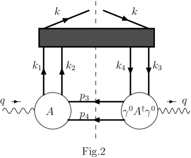
Figure 2: Graphic representation for the contribution in Eq.(4), the broken line is the cut and $k_{4}=k_{1}+k_{2}-k_{3}$.

Since heavy quarks move with a small velocity $v_{Q}$ inside of the baryon in its rest frame, one can use NRQCD to handel heavy quarks, in which a systematic expansion in $v_{Q}$ can be used. Hence, the Fourier transformed matrix element can be expanded in $v_{Q}$ with fields of NRQCD. The relation between NRQCD fields and Dirac field $Q(x)$ in the baryon’s rest frame is

$$Q(x)=e^{-im_{Q}t}\left\{\begin{array}[]{ll}\psi(x)\\ \ 0\end{array}\right\}+{\cal O}(v_{Q})+\cdots,$$ (5)

where $\cdots$ denote the part for antiquark, which is irrelevant here. We will work at the leading order of $v_{Q}$. To express our results for the Fourier transformed matrix element in a covariant way, we denote $v$ as the velocity of the baryon with $v^{\mu}=k^{\mu}/M_{H_{QQ}}$. The Fourier transformed matrix element is then related to that in the rest frame:

$$v^{0}\int d^{4}x_{1}d^{4}x_{2}d^{4}x_{3}e^{-ik_{1}\cdot x_{1}-ik_{2}\cdot x_{2}+ix_{3}\cdot k_{3}}\langle 0|Q_{k}(0)Q_{l}(x_{3})a^{\dagger}({\bf k})a({\bf k})\bar{Q}_{i}(x_{1})\bar{Q}_{j}(x_{2})|0\rangle$$

$$=\int d^{4}x_{1}d^{4}x_{2}d^{4}x_{3}e^{-ik_{1}\cdot x_{1}-ik_{2}\cdot x_{2}+ix_{3}\cdot k_{3}}\langle 0|Q_{k}(0)Q_{l}(x_{3})a^{\dagger}({\bf k}=0)a({\bf k}=0)\bar{Q}_{i}(x_{1})\bar{Q}_{j}(x_{2})|0\rangle.$$ (6)

Using the expansion in Eq.(5) for the matrix element, one will obtain the matrix element containing NRQCD fields $\psi(x)$ and $\psi^{\dagger}(x)$, the space-time of the matrix element with NRQCD fields is controlled by the scale $m_{Q}v_{Q}$ or $\Lambda_{QCD}$, hence at leading order of $v_{Q}$ one can neglect the space-time dependence, also at this order the baryon mass $M_{H_{QQ}}$ is approximated by $2m_{Q}$. With the approximation the matrix element in Eq.(5) is related to the matrix element of NRQCD:

$$\langle 0|\psi^{a_{3}}_{\lambda_{3}}(0)\psi^{a_{4}}_{\lambda_{4}}(0)a^{\dagger}a\psi^{a_{1}\dagger}_{\lambda_{1}}(0)\psi^{a_{2}\dagger}_{\lambda_{2}}(0)|0\rangle,$$ (7)

where we suppressed the notation ${\bf k}=0$ and it is always implied that NRQCD matrix elements are defined in the rest frame of $H_{QQ}$. In the above equation we use $a_{i}(i=1,2,3,4)$ to label the color of quarks fields, while $\lambda_{i}(i=1,2,3,4)$ is for spin indices. The spin indices of the above matrix element runs from $1$ to $2$ because of the structure in Eq.(5). By using rotation invariance, color-symmetry and Pauli principle of two identical fermions the above matrix element is parameterized by two parameters:

$$\langle 0|\psi^{a_{3}}_{\lambda_{3}}\psi^{a_{4}}_{\lambda_{4}}(a^{\dagger}a)\psi^{a_{1}\dagger}_{\lambda_{1}}\psi^{a_{2}\dagger}_{\lambda_{2}}|0\rangle = (\varepsilon)_{\lambda_{4}\lambda_{3}}(\varepsilon)_{\lambda_{2}\lambda_{1}}\cdot(\delta_{a_{1}a_{4}}\delta_{a_{2}a_{3}}+\delta_{a_{1}a_{3}}\delta_{a_{2}a_{4}})\cdot h_{1}$$ (8)

$$\ +(\sigma^{n}\varepsilon)_{\lambda_{4}\lambda_{3}}(\varepsilon\sigma^{n})_{\lambda_{2}\lambda_{1}}\cdot(\delta_{a_{1}a_{4}}\delta_{a_{2}a_{3}}-\delta_{a_{1}a_{3}}\delta_{a_{2}a_{4}})\cdot h_{3},$$

where $\sigma^{i}(i=1,2,3)$ are Pauli matrices, $\varepsilon=i\sigma^{2}$ is totally anti-symmetric. The parameters are defined as:

$$h_{1} = \frac{1}{48}\langle 0|[\psi^{a_{1}}\varepsilon\psi^{a_{2}}+\psi^{a_{2}}\varepsilon\psi^{a_{1}}]a^{\dagger}a\psi^{a_{2}\dagger}\varepsilon\psi^{a_{1}\dagger}|0\rangle,$$

$$h_{3} = \frac{1}{72}\langle 0|[\psi^{a_{1}}\varepsilon\sigma^{n}\psi^{a_{2}}-\psi^{a_{2}}\varepsilon\sigma^{n}\psi^{a_{1}}]a^{\dagger}a\psi^{a_{2}\dagger}\sigma^{n}\varepsilon\psi^{a_{1}\dagger}|0\rangle,$$ (9)

the physical interpretation of parameters is clear: $h_{1}$ represents the probability for a $QQ$ pair in a ${}^{1}S_{0}$ state and in the color state of ${\bf 6}$ to transform into the baryon, while $h_{3}$ represents the probability for a $QQ$ pair in a ${}^{3}S_{1}$ state and in the color state of ${\bf\bar{3}}$ to transform into the baryon. With these results the Fourier transformed matrix element in Eq.(6) can be expressed as:

$$v^{0}\int d^{4}x_{1}d^{4}x_{2}d^{4}x_{3}e^{-ik_{1}\cdot x_{1}-ik_{2}\cdot x_{2}+ix_{3}\cdot k_{3}}\langle 0|Q^{a_{3}}_{k}(0)Q^{a_{4}}_{l}(x_{3})a^{\dagger}({\bf k})a({\bf k})\bar{Q}^{a_{1}}_{i}(x_{1})\bar{Q}^{a_{2}}_{j}(x_{2})|0\rangle$$

$$=(2\pi)^{4}\delta^{4}(k_{1}-m_{Q}v)(2\pi)^{4}\delta^{4}(k_{2}-m_{Q}v)(2\pi)^{4}\delta^{4}(k_{3}-m_{Q}v)$$

$$\ \cdot\big{[}-(\delta_{a_{1}a_{4}}\delta_{a_{2}a_{3}}+\delta_{a_{1}a_{3}}\delta_{a_{2}a_{4}})(\tilde{P}_{v}C\gamma_{5}P_{v})_{ji}(P_{v}\gamma_{5}C\tilde{P}_{v})_{lk}\cdot h_{1}$$

$$\ +(\delta_{a_{1}a_{4}}\delta_{a_{2}a_{3}}-\delta_{a_{1}a_{3}}\delta_{a_{2}a_{4}})(\tilde{P}_{v}C\gamma^{\mu}P_{v})_{ji}(P_{v}\gamma^{\nu}C\tilde{P}_{v})_{lk}(v_{\mu}v_{\nu}-g_{\mu\nu})\cdot h_{3}\big{]}+\cdots,$$ (10)

with

$$P_{v}=\frac{1+\gamma\cdot v}{2},\ \ \ \ \tilde{P}_{v}=\frac{1+\tilde{\gamma}\cdot v}{2}.$$ (11)

In the above equation we used $a_{i}(i=1,2,3,4)$ for the color indices and $ijkl$ for the Dirac indices. $\tilde{A}$ denotes the transpose of the matrix $A$. In Eq.(10) $\cdots$ denote terms at higher orders of $v_{Q}$, which are neglected in this work. These terms as corrections can be systematically added. $C=i\gamma^{2}\gamma^{0}$ is the matrix for charge conjugation. Substituting Eq.(10) into Eq.(4), one can easily find that the two heavy quarks $Q$ are projected to on-shell states and they have the same momentum $m_{Q}v$.

Numerical values of the two matrix elements are unknown yet. There are attempts to relate $h_{3}$ to the corresponding matrix element $|\langle 0|\chi^{\dagger}\mbox{\boldmath$\sigma$}\psi|^{3}S_{1}\rangle|^{2}$ for the transition of a $Q\bar{Q}$ pair into a ${}^{3}S_{1}$ quarkonium, in which one introduces a wave function for ${}^{3}S_{1}$ $QQ$ state, the radial wave function $R_{QQ}(r)$ at origin is related to $h_{3}$ by:

$$h_{3}=\frac{1}{4\pi}|R_{QQ}(0)|^{2}.$$ (12)

Assuming the potentials for binging $Q\bar{Q}$ and $QQ$ state are hydrogen-like, then the difference between the potential for $Q\bar{Q}$ and that for $QQ$ is determined by color structures, using the difference a relation between $R_{QQ}(0)$ and $R_{Q\bar{Q}}(0)$ can be obtained. But such a relation can not be found for $h_{1}$, and the potentials are not exactly hydrogen-like because of QCD confinement. An rough estimation can be obtained by noting that one can give a power counting in $v_{Q}$ for these matrix elements, similarly to the power counting of those matrix elements for quarkonia. For this we note that in general $H_{QQ}$ is a bound state of two heavy quarks $Q$ with other light dynamical freedoms of QCD, the state can be written as:

$$|H_{QQ}\rangle=c_{1}|QQq\rangle+c_{2}|QQqg\rangle+c_{3}|QQqgg\rangle+\cdots.$$ (13)

For a $QQ$ pair in ${}^{3}S_{1}$ state with the color ${\bf\bar{3}}$, one of the heavy quarks can emits a gluon, which does not change the spin of the heavy quark, and this gluon then splits into a $q\bar{q}$. The heavy quark pair can combine the light quark $q$ to form $H_{QQ}$, while $\bar{q}$ will combine other partons to transform into unobserved states. Since the probability of a heavy quark emitting such a gluon is proportional to $v_{Q}$, then we have

$$h_{3}\sim v_{Q}^{2}|\langle 0|\chi^{\dagger}\mbox{\boldmath$\sigma$}\psi|^{3}S_{1}\rangle|^{2}.$$ (14)

For a $QQ$ pair in ${}^{1}S_{0}$ state with the color ${\bf 6}$, if one follows the above discussion by requiring that $H_{QQ}$ is formed by the component $|QQq\rangle$, then the emitted gluon must change the spin of the heavy quark, then one may conclude that $h_{1}$ is at higher order than $v_{Q}^{2}$ in comparison with $h_{3}$. However, $H_{QQ}$ can be formed with the component $|QQqg\rangle$, this component can be formed as the following: One of the heavy quarks emits a gluon, which does not change the spin of the heavy quark, and this gluon splits into a $q\bar{q}$, the light quarks can also emit gluons, then the component can be formed with the light quark $q$ plus one gluon, other light partons are transformed into unobserved state. Unlike for quarkonium systems, in which the leading component is the $Q\bar{Q}$ state, for $H_{QQ}$, all components must contain at least one light quark $q$. Because a light quark can emit gluons easily, the components in Eq.(13) are important at the same level, i.e., $c_{1}\sim c_{2}\sim c_{3}\cdots$. Hence we have:

$$h_{1}\sim v_{Q}^{2}|\langle 0|\chi^{\dagger}\mbox{\boldmath$\sigma$}\psi|^{3}S_{1}\rangle|^{2}.$$ (15)

In deriving the above power counting we basically used perturbative QCD, in general one can not use perturbative QCD to discuss how $H_{QQ}$ is formed, but for power counting in $v_{Q}$ it gives right answers.

With the results in Eq.(10) we obtain the differential cross section:

$$d\sigma = \frac{1}{2\hat{s}}\frac{d^{3}k}{(2\pi)^{3}v_{0}}\int\frac{d^{3}p_{3}}{(2\pi)^{3}2E_{3}}\frac{d^{3}p_{4}}{(2\pi)^{3}2E_{4}}(2\pi)^{4}\delta^{4}(p_{1}+p_{2}-p_{3}-p_{4}-k)$$ (16)

$$\Big{(}\frac{4e^{4}g_{s}^{4}e_{Q}^{2}}{3\hat{s}^{2}}\Big{)}\frac{1}{m_{Q}^{2}}\Big{\{}h_{1}{\cal B}^{(1)}+16h_{3}{\cal B}^{(3)}\Big{\}},$$

where

$${\cal B}^{(i)} = \frac{8}{(1-x_{3})^{2}(1-x_{4})^{2}(x_{3}+x_{4})^{2}}\Big{\{}{\cal A}_{1}^{(i)}+\frac{8(p_{1}\cdot p_{3})^{2}}{s^{2}}{\cal A}_{2}^{(i)}+\frac{8(p_{1}\cdot p_{4})^{2}}{s^{2}}{\cal A}_{2}^{(i)}|_{x_{3}\leftrightarrow x_{4}}$$ (17)

$$+\frac{8(p_{1}\cdot p_{3})(p_{1}\cdot p_{4})}{s^{2}}{\cal A}_{3}^{(i)}+\frac{2(p_{1}\cdot p_{3})}{s}{\cal A}_{4}^{(i)}+\frac{2(p_{1}\cdot p_{4})}{s}{\cal A}_{4}^{(i)}|_{x_{3}\leftrightarrow x_{4}}\Big{\}}.$$

The functions ${\cal A}^{(1,3)}_{i}(i=1,2,3,4)$ depend on $x_{3,4}=2p^{0}_{3,4}/\sqrt{s}$ with $s=(p_{1}+p_{2})^{2}$ and are given in the appendix. Now we take the heavy quark $Q$ as charm quark $c$ to give some numerical results for $\Xi^{+}_{cc}$. It should be noted that the results also apply for $\Xi^{++}_{cc}$ because isospin symmetry. we obtain the total cross section for $e^{+}e^{-}$ colliders at the two B factories with $\sqrt{s}=10.6$ GeV:

$$\sigma=\left\{1.89\left[\frac{h_{1}}{\rm(GeV)^{3}}\right]+7.66\left[\frac{h_{3}}{\rm(GeV)^{3}}\right]\right\}{\rm pb},$$ (18)

for $m_{c}=1.6$GeV and $\alpha_{s}(m_{c})=0.24$. If we take numerical value for $R_{cc}(0)$ estimated in [9] and use Eq.(12), one can get numerical value for the contribution from $h_{3}$. But the contribution from $h_{1}$ is unknown. If we take $h_{1}=h_{3}$, the cross section is $0.23$pb. This value is larger than that estimated in [11]. The reason is that in [11] the contribution of $h_{1}$ is not present. We also calculate the angular distribution and energy distribution, which are given in Fig.3 and Fig.4 respectively, where $\theta_{k}$ is the angle between the moving direction of the $e^{+}$-beam in CMS and that of $H_{QQ}$ and $x_{k}=2k^{0}/\sqrt{s}$. From these figures one can see that the effect of $h_{1}$ is significant, especially in the angular distribution, if $h_{1}$ is not much smaller than $h_{3}$.

Our numerical results should be understood as rough estimations, because the exact values of $h_{1}$ and $h_{3}$ are unknown. With the definitions of these parameters in Eq.(9) one can use nonperturbative methods to study them, or they can be extracted from experimental results because they are universal. Once they are known, accurate results can be given with our results.

Figure 3: Results for the distribution $\frac{1}{\sigma}\frac{d\sigma}{dcos\theta_{k}}$. The solid line is for $h_{3}=0$, the dotted is for $h_{1}=0$ and the dash-dotted is for $h_{1}=h_{3}$.

Figure 4: Results for $\frac{1}{\sigma}\frac{d\sigma}{dx_{k}}$. The solid line is for $h_{3}=0$, the dotted is for $h_{1}=0$ and the dash-dotted is for $h_{1}=h_{3}$.

3. Heavy Quark Fragmentation

In this section we will use the factorization approach to calculate the fragmentation function of a heavy quark $Q$ into a doubly heavy baryon $H_{QQ}$. We will calculate the function by starting from its definition[12]. To give the definitions for a fragmentation function it is convenient to work in the light-cone coordinate system. In this coordinate system a 4-vector $p$ is expressed as $p^{\mu}=(p^{+},p^{-},{\bf p_{T}})$, with $p^{+}=(p^{0}+p^{3})/\sqrt{2},\ p^{-}=(p^{0}-p^{3})/\sqrt{2}$. Introducing a vector $n$ with $n^{\mu}=(0,1,{\bf 0_{T}})$, the fragmentation function can be defined in the light cone gauge $n\cdot G(x)=0$ as[12]:

$$D_{H_{QQ}/Q}(z) = \frac{z}{4\pi}\int dx^{-}e^{-ik^{+}x^{-}/z}\frac{1}{3}{\rm Tr_{color}}\frac{1}{2}{\rm Tr_{Dirac}}$$ (19)

$$\cdot\{n\cdot\gamma\langle 0|Q(0)a_{H}^{\dagger}(k^{+},{\bf 0_{T}})a(k^{+},{\bf 0_{T}})\bar{Q}(0,x^{-},{\bf 0_{T}})|0\rangle\},$$

where $G_{\mu}(x)=G^{a}_{\mu}(x)T^{a}$, $G_{\mu}^{a}(x)$ is the gluon field and the $T^{a}(a=1,\dots,8)$ are the color matrices. The summation over the spin of $H_{QQ}$ is implied. In other gauges gauge links must be supplied to make the definition gauge invariant. The function $D_{H/QQ}(z)$ is interpreted as the probability of a quark $Q$ with momentum $p$ to decay into the hadron $H$ with momentum component $k^{+}=zp^{+}$. The function is invariant under a Lorentz boost along the $z$-direction. Hence we can calculate the function in the rest frame of $H_{QQ}$. It should be noted that the above definition is given with relativistic normalization of states. Starting definitions of fragmentation functions, various fragmentation functions for quarkonia have been calculated[13, 14, 15]. In the case of doubly heavy baryon the calculation is similar.

Figure 5: Graphic representation for fragmentation function.

At tree-level, the fragmentation can be understood as the following: The heavy quark generates a heavy quark pair through exchange of a hard gluon, the two heavy quarks will be combined with other partons generated nonperturbatively into the baryon. This contribution is illustrated in Fig.5. It is straightforward to write down the contribution to the function from its definition:

$$D_{H_{QQ}/Q}(z) = \frac{zg_{s}^{4}}{24\pi}\int dx^{-}e^{-ip^{+}x^{-}/z}\int\frac{d^{4}p_{1}}{(2\pi)^{4}}2\pi\delta(p_{1}^{2}-m_{Q}^{2})$$ (20)

$$\cdot\int d^{4}x_{1}d^{4}x_{2}d^{4}y_{1}d^{4}y_{2}e^{ip_{1}\cdot x_{1}}\langle 0|\bar{Q}_{i}(x_{1})\bar{Q}_{j}(x)[a^{\dagger}a]Q_{k}(y_{1})Q_{l}(y_{2})|0\rangle$$

$$\cdot(\gamma^{\mu_{1}}T^{a}(\gamma\cdot p_{1}-m_{Q})\gamma^{\mu_{2}}T^{b})_{il}(\gamma^{\nu_{1}}T^{a}S(x_{2},x)\gamma\cdot nS(0,y_{1})\gamma^{\nu_{2}}T^{b})_{jk}$$

$$\cdot D_{\mu_{1}\nu_{1}}(x_{1},x_{2})\cdot D_{\mu_{2}\nu_{2}}(y_{2},y_{1}),$$

where $x^{\mu}=(0,x^{-},{\bf 0_{T}})$. $iS(x,y)$ is the quark propagator of $Q$, while $-iD_{\mu\nu}(x,y)$ is the gluon propagator in the light cone gauge. By using the results for the matrix element obtained before, we obtain:

$$D_{H_{QQ}}(z,\mu) = \alpha_{s}^{2}(\mu)\frac{z(1-z)^{2}}{(2-z)^{6}}\cdot\{\frac{8h_{1}}{27m_{Q}^{3}}(3z^{4}-8z^{3}+8z^{2}+48)$$ (21)

$$+\frac{16h_{3}}{9m_{Q}^{3}}(5z^{4}-32z^{3}+72z^{2}-32z+16)\}.$$

The calculation can be done in the rest frame of $H_{QQ}$ straightforwardly, where we have to convert the matrix element in Eq.(20) through the factor $4m_{Q}$ into that with nonrelativistic normalization. The term with $h_{3}$ is also calculated in [6], it is the same as ours.

With these results, one can estimate the production rate at a hadron collider like Tevatron and LHC. The rate can be estimated as:

$$\sigma_{H_{QQ}}(p_{t})\approx\sigma_{Q}(p_{t})\cdot M_{Q}^{(1)}(p_{t}),$$ (22)

where $\sigma_{H_{QQ}}(p_{t})$ and $\sigma_{Q}(p_{t})$ is the cross section for inclusive production of $H_{QQ}$ and $Q$ with transverse momentum larger than $p_{t}$, respectively. $M_{Q}^{(1)}(p_{t})$ is the first moment of the fragmentation function at the energy scale $\mu=p_{t}$. To avoid large logarithm like $\ln{p_{t}/m_{Q}}$ in our perturbative result of $D_{H_{QQ}}$, one can use renormalization group method to sum these large log terms. But, if in the summation one neglects the gluon fragmentation which is at least at order of $\alpha_{s}^{3}$ and uses one loop result for anomal dimensions, then the first moment does not change with the scale $\mu$. We use $\alpha_{s}(\mu)$ at $\mu=m_{c}$ for calculating the first moment. $\sigma_{Q}(p_{t})$ is calculated at tree-level by taking two partonic processes $q\bar{q}\rightarrow Q\bar{Q}$ and $gg\rightarrow Q\bar{Q}$. Taking $p_{t}=40$GeV, $m_{c}=1.6$GeV and $\alpha_{s}(m_{c})=0.24$ we obtain for LHC and Tevatron:

$$\sigma_{\Xi^{+}_{cc}} \simeq \Big{\{}0.0014\Big{[}\frac{h_{1}}{(GeV)^{3}}\Big{]}+0.0029\Big{[}\frac{h_{3}}{(GeV)^{3}}\Big{]}\Big{\}},~{}~{}~{}~{}{\rm for~{}Tevatron},$$

$$\sigma_{\Xi_{cc}^{+}} \simeq \Big{\{}0.020\Big{[}\frac{h_{1}}{(GeV)^{3}}\Big{]}+0.042\Big{[}\frac{h_{3}}{(GeV)^{3}}\Big{]}\Big{\}},~{}~{}~{}~{}{\rm for~{}LHC}.$$ (23)

If we take the same value of $h_{3}$ as in the last section and $h_{1}=h_{3}$, we obtain $\sigma_{\Xi^{+}_{cc}}=0.0018$mb for LHC and $\sigma_{\Xi^{+}_{cc}}=0.00013$mb for Tevatron, respectively. With the planed luminosity $100({\rm fb})^{-1}$ per year of LHC there will $1.8=\times 10^{11}$ $\Xi^{+}_{cc}$’s produced at LHC. Our numerical results are roughly 10 times larger than those estimated in [9]. Beside the extra contribution from $h_{1}$, one main reason for this is that our estimations are sensitive to values of parameters. If we take $m_{c}=1.7$GeV and $\alpha_{s}=0.2$ as taken in [9], our numerical results will become 10 times smaller. It is interesting to note that our numerical results roughly remain the same if we take $p_{t}=10$GeV. However, our estimation for $p_{t}=10$GeV or smaller $p_{t}$ can not be reliable, because contributions from fragmentation are dominant at high $p_{t}$ and other contributions are significant at low $p_{t}$. Including all contributions one is able to show that contributions from fragmentation become dominant for $p_{t}\sim 25-30$GeV[9].

4. Summary

We have studied inclusive production of doubly heavy baryon $H_{QQ}$ at a $e^{+}e^{-}$ collider and through fragmentation of a heavy quark, in which a factorization was performed to factorize perturbative- and nonperturbative effects. In our approach the production can be understood as a two-step process, in which a $QQ$ pair is produced first and then the pair is transformed into $H_{QQ}$ nonperturbatively. The production of the $QQ$ pair can be studied with perturbative QCD because the large mass $m_{Q}$. With the large mass $m_{Q}$ a heavy quark $Q$ moves with a small velocity $v_{Q}$ in $H_{QQ}$ in its rest frame. This suggests that one can use NRQCD to describe the transformation, where a systematic expansion in $v_{Q}$ can be performed. At the leading order we find that $H_{QQ}$ can be formed from two states of the $QQ$ pair, one state is with the pair in ${}^{3}S_{1}$ state and in color ${\bf\bar{3}}$, another is with the pair in ${}^{1}S_{0}$ state and in color ${\bf 6}$. The transformation from these two states are described by two matrix elements $h_{1}$ and $h_{3}$, defined with NRQCD. A power counting in $v_{Q}$ for these two matrix elements is given. Our results are different than those in previous approaches, where $H_{QQ}$ is formed only from the state of the pair in ${}^{3}S_{1}$ state and in color ${\bf\bar{3}}$. Perturbative coefficients in the contributions of these two states to the production at $e^{+}e^{-}$ colliders and to the production through heavy quark fragmentation are calculated at tree-level.

Numerical results are given for $\Xi^{+}_{cc}$-production at B-factories and for $\Xi^{+}_{cc}$-production through fragmentation at LHC and Tevatron, in which we relate the parameter $h_{3}$ to a wave function of the $cc$ pair, which has been studied and results are given for different ratios $h_{1}/h_{3}$. We find that the contribution of $h_{1}$, i.e., of the state of the $cc$ pair in ${}^{1}S_{0}$ state and in color ${\bf 6}$, is significant, if $h_{1}$ is not much smaller than $h_{3}$. It should be noted that detailed values of the two matrix elements are unknown, our numerical results should be taken as rough estimations. The two matrix elements can be studied by nonperturbative methods, or extracted from experiment. If their values are known, detailed predictions can be made.

Acknowledgements

This work is supported by National Nature Science Foundation of P. R. China.

Appendix

The functions in the differential cross section are:

$${\cal A}_{1}^{(1)} = -\frac{32m_{Q}^{6}\Big{[}4(1-x_{3}-x_{4})+(x_{3}^{2}+x_{4}^{2})+x_{3}x_{4}(4-x_{3}-x_{4})\Big{]}^{2}}{\hat{s}^{3}(1-x_{3})^{2}(1-x_{4})^{2}}+\frac{16m_{Q}^{4}}{\hat{s}^{2}(1-x_{3})^{2}(1-x_{4})^{2}}\Big{\{}32$$

$$-88(x_{3}+x_{4})+78(x_{3}^{2}+x_{4}^{2})-16(x_{3}^{3}+x_{4}^{3})-16(x_{3}^{4}+x_{4}^{4})+12(x_{3}^{5}+x_{4}^{5})-3(x_{3}^{6}+x_{4}^{6})$$

$$+x_{3}x_{4}\Big{[}228-192(x_{3}+x_{4})+44(x_{3}^{2}+x_{4}^{2})+20(x_{3}^{3}+x_{4}^{3})-12(x_{3}^{4}+x_{4}^{4})+2(x_{3}^{5}+x_{4}^{5})$$

$$+x_{3}x_{4}[168-56(x_{3}+x_{4})+(x_{3}^{2}+x_{4}^{2})+2(x_{3}^{3}+x_{4}^{3})+4x_{3}x_{4}7-x_{3}-x_{4})]\Big{]}\Big{\}}$$

$$+\frac{2m_{Q}^{2}}{\hat{s}(1-x_{3})(1-x_{4})}\Big{\{}-64+160(x_{3}+x_{4})-116(x_{3}^{2}+x_{4}^{2})+24(x_{3}^{3}+x_{4}^{3})+7(x_{3}^{4}+x_{4}^{4})$$

$$-3(x_{3}^{5}+x_{4}^{5})+x_{3}x_{4}\Big{[}-360+216(x_{3}+x_{4})-24(x_{3}^{2}+x_{4}^{2})-11(x_{3}^{3}+x_{4}^{3})+3(x_{3}^{4}+x_{4}^{4})$$

$$-2x_{3}x_{4}[55-7(x_{3}+x_{4})+2(x_{3}^{2}+x_{4}^{2})-x_{3}x_{4}]\Big{]}\Big{\}}+(x_{3}-x_{4})^{2}\Big{\{}-6+10(x_{3}+x_{4})$$

$$-5(x_{3}^{2}+x_{4}^{2})+(x_{3}^{3}+x_{4}^{3})-x_{3}x_{4}(8-x_{3}-x_{4})\Big{\}},$$

$${\cal A}_{2}^{(1)} = -\frac{16m_{Q}^{4}\Big{[}2-2x_{3}+x_{3}^{2}-x_{4}^{2}\Big{]}^{2}}{\hat{s}^{2}(1-x_{3})^{2}}+\frac{8m_{Q}^{2}}{\hat{s}(1-x_{3})}\Big{\{}6-x_{3}(10-9x_{3}+3x_{3}^{2})-x_{4}(4+3x_{4}$$

$$-2x_{4}^{2})+x_{3}x_{4}(2+x_{4})\Big{\}}-x_{3}^{2}(1-x_{3})-x_{4}^{2}(5-3x_{4}+x_{4}^{2})-x_{3}x_{4}\Big{[}-6+x_{4}-2x_{4}^{2}$$

$$+x_{3}(3+x_{4})\Big{]},$$

$${\cal A}_{3}^{(1)} = 2\Big{\{}8(x_{3}+x_{4}-1)-3(x_{3}^{2}+x_{4}^{2})+x_{3}x_{4}[(x_{3}-x_{4})^{2}-2]\Big{\}}+\frac{16m_{Q}^{2}}{\hat{s}(1-x_{3})(1-x_{4})}\Big{\{}\frac{2m_{Q}^{2}}{\hat{s}}\Big{[}$$

$$4(x_{3}+x_{4}-1)+(x_{4}^{4}+x_{3}^{4})-2(x_{3}^{3}+x_{4}^{3})+2x_{3}x_{4}(x_{3}+x_{4}-2-x_{3}x_{4})\Big{]}+6-10(x_{3}$$

$$+x_{4})+4(x_{3}^{2}+x_{4}^{2})+2(x_{3}^{3}+x_{4}^{3})-(x_{3}^{4}+x_{4}^{4})+2x_{3}x_{4}[7-3(x_{3}+x_{4})+x_{3}x_{4}]\Big{\}},$$

$${\cal A}_{4}^{(1)} = 2(1-x_{3})\Big{[}x_{3}^{3}+x_{4}(8-8x_{4}+3x_{4}^{2})-x_{3}x_{4}(3x_{3}+x_{4})\Big{]}+\frac{16m_{Q}^{2}}{\hat{s}(1-x_{3})(1-x_{4})}\Big{\{}$$ (24)

$$\frac{2m_{Q}^{2}}{\hat{s}(1-x_{3})}\Big{[}x_{3}(2-2x_{3}+x_{3}^{2})^{2}+x_{4}(4-4x_{4}+2x_{4}^{3}-x_{4}^{4})-x_{3}x_{4}[12-x_{3}(12-6x_{3}$$

$$+x_{3}^{2})-x_{4}(4-2x_{4}+x_{4}^{2})+2x_{3}x_{4}]\Big{]}-x_{3}[6-10x_{3}+9x_{3}^{2}-3x_{3}^{3}]-x_{4}(6-10x_{4}$$

$$+4x_{4}^{2}+2x_{4}^{3}-x_{4}^{4})+x_{3}x_{4}\Big{[}20-x_{3}(16-7x_{3}+2x_{3}^{2})+x_{4}(2x_{4}^{2}+x_{4}-15)$$

$$+x_{3}x_{4}(7-x-4)\Big{]}\Big{\}}.$$

$${\cal A}_{1}^{(3)} = \frac{2m_{Q}^{4}}{\hat{s}^{2}(1-x_{3})^{2}(1-x_{4})^{2}}\Big{\{}\frac{2m_{Q}^{2}}{\hat{s}}\Big{[}-64+144(x_{3}+x_{4})-100(x_{3}^{2}+x_{4}^{2})+20(x_{3}^{4}+x_{4}^{4})$$

$$-3(x_{3}^{6}+x_{4}^{6})+x_{3}x_{4}\Big{(}-328+2[128(x_{3}+x_{4})-28(x_{3}^{2}+x_{4}^{2})-8(x_{3}^{3}+x_{4}^{3})$$

$$+3(x_{3}^{4}+x_{4}^{4})])-x_{3}x_{4}[216+x_{3}^{2}+x_{4}^{2}-64(x_{3}+x_{4})+20x_{3}x_{4}]\Big{)}\Big{]}+32-104(x_{3}+x_{4})$$

$$+118(x_{3}^{2}+x_{4}^{2})-50(x_{3}^{3}+x_{4}^{3})-28(x_{3}^{4}+x_{4}^{4})+46(x_{3}^{5}+x_{4}^{5})-17(x_{3}^{6}+x_{4}^{6})+x_{3}x_{4}\Big{[}228$$

$$-158(x_{3}+x_{4})+44(x_{3}^{2}+x_{4}^{2})+18(x_{3}^{3}+x_{4}^{3})-36(x_{3}^{4}+x_{4}^{4})+14(x_{3}^{5}+x_{4}^{5})-x_{3}x_{4}[-32$$

$$+8(x_{3}+x_{4})-23(x_{3}^{2}+x_{4}^{2})+4(x_{3}^{3}+x_{4}^{3})+2x_{3}x_{4}(5(x_{3}+x_{4})-6)]\Big{]}\Big{\}}+(x_{3}-x_{4})^{2}\Big{[}$$

$$(x_{3}^{3}+x_{4}^{3})-3(x_{3}^{2}+x_{4}^{2})+4(x_{3}+x_{4})+3x_{3}x_{4}[x_{3}+x_{4}-2]-2\Big{]}-\frac{m_{Q}^{2}}{\hat{s}(1-x_{3})(1-x_{4})}\Big{\{}$$

$$12(x_{3}^{2}+x_{4}^{2})-37(x_{3}^{3}+x_{4}^{3})+42(x_{3}^{4}+x_{4}^{4})-17(x_{3}^{5}+x_{4}^{5})+2(x_{3}^{6}+x_{4}^{6})+x_{3}x_{4}\Big{[}7x_{3}^{4}$$

$$+7x_{4}^{4}-36(x_{3}^{3}+x_{4}^{3})+34(x_{3}^{2}+x_{4}^{2})-3(x_{3}+x_{4})+x_{3}x_{4}[4(x_{3}^{2}+x_{4}^{2})+5(x_{3}+x_{4})$$

$$+6x_{3}x_{4}-32]\Big{]}\Big{\}},$$

$${\cal A}_{2}^{(3)} = \frac{m_{Q}^{2}}{\hat{s}(1-x_{3})}\Big{\{}\frac{2m_{Q}^{2}}{\hat{s}(x_{3}-1)}\Big{[}12+3x_{3}^{4}-16x_{3}^{3}+36x_{3}^{2}-32x_{3}+3x_{4}^{4}-4x_{4}^{3}-8x_{4}$$

$$+2x_{3}x_{4}[2x_{3}^{2}+x_{3}(x_{4}-10)+2(6-2x_{4}+x_{4}^{2})\Big{]}+\frac{1}{1-x_{4}}\Big{[}4-2x_{3}(x_{3}^{3}-x_{3}^{2}-3x_{3}+6)$$

$$-x_{4}(12-16x_{4}+3x_{4}^{2}+9x_{4}^{3}-6x_{4}^{4})+x_{3}x_{4}\Big{(}14+x_{3}(x_{3}-5)-x_{4}(10-5x_{4}+x_{4}^{2})$$

$$+x_{3}x_{4}(5+x_{3}-6x_{4})\Big{)}\Big{]}\Big{\}}+(x_{3}-x_{4})^{2}(x_{3}+x_{4}-1),$$

$${\cal A}_{3}^{(3)} = 2(x_{3}-x_{4})^{2}(x_{3}+x_{4}-1)+\frac{m_{Q}^{2}}{\hat{S}(1-x_{3})(1-x_{4})}\Big{\{}\frac{4m_{Q}^{2}}{\hat{s}}\Big{[}5(x_{3}^{4}+x_{4}^{4})-16(x_{3}^{3}+x_{4}^{3})$$

$$+22(x_{3}^{2}+x_{4}^{2})-12(x_{3}+x_{4})-4+2x_{3}x_{4}[20-12(x_{3}+x_{4})+3(x_{3}^{2}+x_{4}^{2})+x_{3}x_{4}]\Big{]}$$

$$+2(x_{3}^{5}+x_{4}^{5})-3(x_{3}^{4}+x_{4}^{4})+9(x_{3}^{3}+x_{4}^{3})-20(x_{3}^{2}+x_{4}^{2})+16(x_{3}+x_{4})-x_{3}x_{4}\Big{[}72$$

$$+5(x_{3}^{3}+x_{4}^{3})+4(x_{3}^{2}+x_{4}^{2})-55(x_{3}+x_{4})+x_{3}x_{4}[34-3(x_{3}+x_{4})]\Big{]}\Big{\}},$$

$${\cal A}_{4}^{(3)} = -2(x_{3}-x_{4})^{2}\Big{[}x_{3}^{2}-(1-x_{4})x_{4}-x_{3}(1-2x_{4})\Big{]}+\frac{m_{Q}^{2}}{\hat{s}(1-x_{3})(1-x_{4})}\Big{\{}\frac{4m_{Q}^{2}}{\hat{s}(1-x_{3})}\Big{[}(12$$ (25)

$$-32x_{3}+36x_{3}^{2}-16x_{3}^{3}+3x_{3}^{4})x_{3}+x_{4}(4+12x_{4}-22x_{4}^{2}+16x-4^{3}-5x_{4}^{4})$$

$$+x_{3}x_{4}\Big{(}-12+x_{3}[22-18x_{3}-x_{3}^{2}+2x_{3}^{3}]+x_{4}[-44+42x_{4}-15x_{4}^{2}+2x_{4}^{3}]$$

$$+2x_{3}x_{4}[16-4x_{3}+x_{3}^{2}-7x_{4}+x_{4}^{2}]\Big{)}\Big{]}+4x_{3}[-2+6x_{3}-3x_{3}^{2}-x_{3}^{3}+x_{3}^{4}]+x_{4}^{2}[-16$$

$$+20x_{4}-9x_{4}^{2}+3x_{4}^{3}-2x_{4}^{4}]+x_{3}x_{4}\Big{(}8+x_{3}[-8+x_{3}+x_{3}^{2}-2x_{3}^{3}]+x_{4}[40-49x_{4}+22x_{4}^{2}$$

$$-7x_{4}^{3}]+x_{3}x_{4}[-35+9x_{3}x_{4}-3x_{3}(2-x_{3})+x_{4}(24-x_{4})\Big{)}\Big{\}}.$$

References

[1] N. Isgur and M.B. Wise, Phys. Lett. B232 (1989) 113, ibid.
B237 (1990) 527,
E. Eichten and B. Hill, Phys. Lett. B234 (1990) 511,
B. Grinstein, Nucl. Phys. B339 (1990) 253,
H. Georgi, Phys. Lett. B240 (1990) 447.
[2]G.T. Bodwin, E. Braaten, and G.P. Lepage,
Phys. Rev. D51, 1125 (1995); Erratum:ibid., D55,
5853 (1997).
[3] G.P. Lepage, L. Magnea, C. Nakhleh, U. Magnea and K. Hornbostel,
Phys. Rev. D46 (1992) 4052
[4] M. Mattson et al., Selex Collaboration, Phys. Rev. Lett. 89
(2002) 112001
[5] V.V. Kiselev and A.K. Likhoded,
Comment on ”First observation of doubly charmed baryon ”,
hep-ph/0208231
[6] A.F. Falk, M. Luke, M.J. Savage and M.B. Wise, Phys. Rev. D49
(1994) 555
[7] V.V. Kiselev, A.K. Likhoded and M.V. Shevlyagin, Phys. Lett. B332
(1994) 411
[8] A.V. Berezhnoy, V.V. Kiselev and A.K. Likhoded, Phys. At. Nucl.
59 (1996) 870
[9] A.V. Berezhnoy, V.V. Kiselev, A.K. Likhoded and I. Onishchenko,
Phys. Rev. D57 (1998) 4385
[10] S.P. Baranov, Phys. Rev. D54 (1996) 3228
[11] A.V. Berezhnoy and A.K. Likhoded, hep-ph/0303145