SLAC-PUB-9731 May 2003

Kaluza-Klein/$Z^{\prime}$ Differentiation at the LHC and Linear Collider

Thomas.G. Rizzo

Stanford Linear Accelerator Center, Stanford, CA, 94309

We explore the capabilities of the LHC and the Linear Collider(LC) to distinguish the production of Kaluza-Klein(KK) excitations from an ordinary $Z^{\prime}$ within the context of theories with TeV scale extra dimensions. At the LHC, these states are directly produced in the Drell-Yan channel while at the LC the effects of their exchanges are indirectly felt as new contact interactions in processes such as $e^{+}e^{-}\rightarrow f\bar{f}$. While we demonstrate that the LC is somewhat more capable at KK/$Z^{\prime}$ differentiation than is the LHC, the simplest LC analysis relies upon the LHC data for the resonance mass as an important necessary input.

1 Introduction and An Outline of the Problem

The possibility of KK excitations of the Standard Model(SM) gauge bosons within the framework of theories with TeV-scale extra dimensions has been popular for some time[1]. The proven variety of such models is very large and continues to grow. For example, given the possibility of warped or flat extra dimensions one can construct a large number of interesting yet distinct models whose detailed structure depends upon a number of choices, e.g., whether all the gauge fields experience the same number of dimensions, whether the fermions and/or Higgs bosons are also in the bulk, whether brane kinetic terms are important[2] in the determination of the KK spectrum and couplings and whether there exists a conservation law of KK number or KK parity, as in the case of the Universal Extra Dimensions(UED)[3] scenario. If such KK gauge excitations do exist how will they be observed at colliders and how will we know that we have observed signals for extra dimensions and not some other new physics signature? For example, it is well known that UED might be mimicked by supersymmetry with somewhat degenerate superpartners at the LHC[3] unless the spins of the new KK states can be measured as can be done at the LC or the higher KK modes observed.

In the analysis below we will be interested in the question of distinguishing the lightest KK excitations of the SM electroweak gauge bosons from a more conventional $Z^{\prime}$ at both the LHC and LC. At the LHC, single KK/$Z^{\prime}$ production is most easily observed via the Drell-Yan mechanism whereas, at the LC, the exchange of either set of states leads to contact interaction-like modifications to processes such as $e^{+}e^{-}\rightarrow f\bar{f}$. Here we will assume that the LHC discovers a single, rather heavy KK state whose mass is beyond the direct reach of the LC, a possibility consistent with the simplest TeV^-1 extra dimensions scenario. The state is assumed to be sufficiently massive, as indicated by current constraints from precision measurements, so that higher KK states cannot be produced thus eliminating the most obvious signature for KK production Though other scenarios are of course possible, the one considered here is the simplest case to analyse; more complex possibilities will be studied elsewhere.

The nature of our question and the above assumptions already limit our focus to a rather specific class of extradimensional theories and excludes many others. For example, at the tree level in UED, a conserved KK-parity exists which forbids the single production or exchange of KK states by zero modes and thus this class of theories is clearly excluded from our considerations. (We note, however, that at one loop the production of the even members of the KK tower are allowed by KK-parity conservation. The UED case and the standard $Z^{\prime}$ scenario can then be most easily distinguished by the existence of the set of first KK excitations with masses essentially half that of the KK state observed in Drell-Yan.) In addition we can exclude models whose couplings and spectra are such that multiple KK resonances will be directly observable at the LHC. In this case there can be no issue of confusion as to whether or not extradimensional signatures are being produced (unless one is willing to postulate the existence of a conspiratorial multi-$Z^{\prime}$ model). We also can exclude from consideration the set of models wherein the KK excitations of only the $SU(2)_{L}$ or $U(1)_{Y}$ gauge bosons can be produced. If either of these possibilities were realized and the spectrum of the KK fields was such that second and higher resonances were beyond the reach of the LHC, one can easily convince oneself that the KK and $Z^{\prime}$ interpretations cannot be distinguished. (Of course the LC would tell us the couplings of these states and identify them as ‘copies’ of those in the SM.) A similar situation holds for $W^{\pm}$ KK excitations even when the entire $SU(2)_{L}\times U(1)_{Y}$ gauge structure is in the bulk since there are only one set of KK excitations in this channel. Of course after making these few cuts in model space many theories remain to be examined and a full analysis of all the possibilities is beyond the scope of this paper.

The simplest model of the class we will consider is the case of only one flat extra dimension; a generalization of our analysis to some of the more complex scenarios will be considered elsewhere. In this basic scheme all the fermions are constrained to lie at one of the two orbifold fixed points, $y=0,\pi R$, associated with the compactification on the orbifold $S^{1}/Z_{2}$[4], where $R$ is the radius of the compactified extra dimension. Under usual circumstances a 3-brane is located at each of the fixed points upon which ordinary 4-d fields will reside. In principle, a SM fermion can be localized on the brane at either fixed point consistent with the constraints of gauge invariance. In our discussions below we will consider two specific cases: either all of the fermions are placed at $y=0$($D=0$), the standard situation, or the quarks and leptons are localized at opposite fixed points($D=\pi R$). Here $D$ is the distance between the quarks and leptons in the single extra dimension. The latter model, with oppositely localized quarks and leptons may be of interest in the suppression of proton decay in certain schemes. (Certainly more complicated scenarios are possible even if we assume generation independence and natural flavor conservation.) In such schemes the fermionic couplings of the KK excitations of a given gauge field are identical to those of the SM, apart from a possible sign if the relevant fermion under consideration lives at the $y=\pi R$ fixed point, and an overall factor of $\sqrt{2}$. The gauge boson KK excitation masses are given, to lowest order in $(M_{0}/M_{c})^{2}$, by the relationship $M_{n}^{2}=(nM_{c})^{2}+M_{0}^{2}$, where $n$ labels the KK level, $M_{c}=1/R\sim 1$ TeV is the compactification scale and $M_{0}$ is the zero-mode mass obtained via spontaneous symmetry breaking for the cases of the $W$ and $Z$. Here we have assumed that any brane localized kinetic terms which may be present[2] do not significantly alter these naive results. Note that the first KK excitations of the photon and $Z$ will be highly degenerate in mass, becoming more so as $M_{c}$ increases. For example, if $M_{c}=4$ TeV the splitting between the first $Z$ and $\gamma$ KK states is less than $\sim$ 1 GeV, too small to be observed at the LHC.

An updated analysis[4] of precision electroweak data implies that $M_{c}\mathrel{\mathchoice{\lower 3.01385pt\vbox{\halign{$\matth\displaystyle\hfil#\hfil$\cr>\crcr\sim\crcr}}}{\lower 3.01385pt\vbox{\halign{$\matth\textstyle\hfil#\hfil$\cr>\crcr\sim\crcr}}}{\lower 3.01385pt\vbox{\halign{$\matth\scriptstyle\hfil#\hfil$\cr>\crcr\sim\crcr}}}{\lower 3.01385pt\vbox{\halign{$\matth\scriptscriptstyle\hfil#\hfil$\cr>\crcr\sim\crcr}}}}4-5$ TeV, independently of whether the Higgs field vev is mostly in the bulk or on the brane or upon which of the fixed points the various SM fermions are confined. This is a mass range directly accessible to the LHC for resonance production in the Drell-Yan channel. Interestingly, at a LC with a center of mass energy of $\sqrt{s}=500-1000$ GeV the effects of KK exchanges with masses well in excess of the $M_{c}\sim 4-5$ TeV range are also easily observable as is shown in Fig. 1. This implies that there will be sufficient ‘resolving power’ at an LC to examine the influence of somewhat smaller values of $M_{c}$ in detail.

Of course this large value of $M_{c}$ implies that the LHC experiments will at best observe only a single bump in the $\ell^{+}\ell^{-}$ channel as the next set of KK states, which are essentially twice as heavy, $\mathrel{\mathchoice{\lower 3.01385pt\vbox{\halign{$\matth\displaystyle\hfil#\hfil$\cr>\crcr\sim\crcr}}}{\lower 3.01385pt\vbox{\halign{$\matth\textstyle\hfil#\hfil$\cr>\crcr\sim\crcr}}}{\lower 3.01385pt\vbox{\halign{$\matth\scriptstyle\hfil#\hfil$\cr>\crcr\sim\crcr}}}{\lower 3.01385pt\vbox{\halign{$\matth\scriptscriptstyle\hfil#\hfil$\cr>\crcr\sim\crcr}}}}8-10$ TeV, are too massive to be seen even with an integrated luminosity of order $1-3$ $ab^{-1}$[5]. (Such high luminosities may be approachable at an upgrade of the LHC[11]; we will keep this possibility in mind in our analysis below.) This can be seen from Fig. 2 which follows from assumptions that all fermions lie at either the $y=0$ or $y=\pi R$ fixed points, i.e., $D=0$ or $\pi R$. These apparently isolated single resonance structures are, of course, superpositions of the individual excitations of both the SM $\gamma$ and $Z$ which are highly degenerate as we noted above. It is this dual excitation plus the existence of additional tower states that lead to the very unique resonance shapes that we see in either case. Note that above the first KK resonance the excitation curves for the $D=0$ and $\pi R$ cases are essentially identical. This figure shows that KK states up to masses somewhat in excess of $\simeq 7$ TeV or so should be directly observable at the LHC or the LHC with a luminosity upgrade in a single lepton pair channel.

It is important to note that if brane kinetic terms, we have so far ignored, are important then the bounds on $M_{c}$ from precision measurements can be significantly weaker due to reduced fermion-KK gauge couplings thus allowing for a much lighter first KK state. It may then be possible to directly observe the higher excitations so that no confusion with $Z^{\prime}$ production would occur. However, parameter space regions may exist where such a possibility would not occur though the first excitation remains light; such scenarios are beyond the scope of the present analysis and will be considered elsewhere.

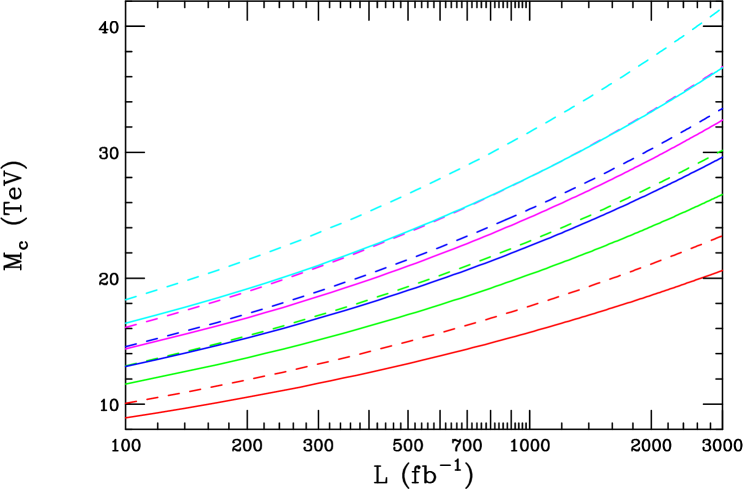
Figure 1: $95\%$ CL bound on the scale $M_{c}$ as a function of the LC integrated luminosity from the reaction $e^{+}e^{-}\rightarrow f\bar{f}$, where $f=\mu,\tau,c,b,t$ have been summed over. The solid(dashed) curves assume a positron polarization $P_{+}=0(0.6)$; an electron polarization of $80\%$ has been assumed in all cases. From bottom to top the center of mass energy of the LC is taken to be 0.5, 0.8, 1, 1,2 and 1.5 TeV, respectively.

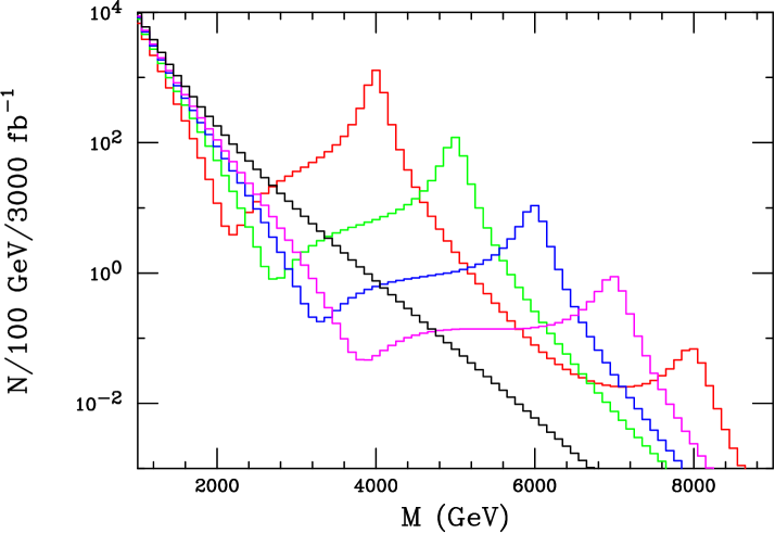
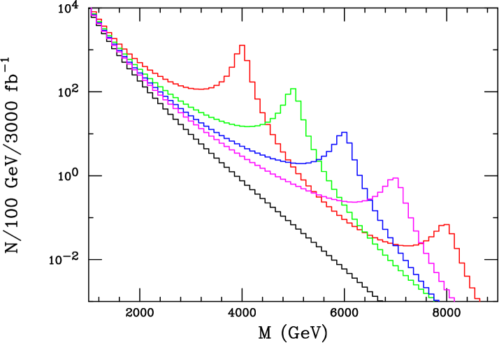
Figure 2: Production rate, in the Drell-Yan channel $pp\rightarrow e^{+}e^{-}X$, for $\gamma/Z$ KK resonances as a function of dilepton invariant mass assuming a very high luminosity LHC. A rapidity cut $|\eta_{l}|\leq 2.5$ has been applied to the final state leptons. The red(green, blue, magenta) histogram corresponds $M_{c}$=4(5, 6, 7) TeV, respectively. The black histogram is the SM background. In the top panel all fermions are assumed to lie at the $y=0$ fixed point, $D=0$, while the quarks and leptons are split, $D=\pi R$, in the lower panel.

If a gauge KK resonance structure is observed in Drell-Yan, how will this observation be interpreted? Here we imagine a time line where the LC turns on after several years of data taking by the LHC at roughly the time of an LHC luminosity upgrade. Through straightforward measurement of the lepton pair angular distribution it will be known immediately that the resonance is spin-1 and not, e.g., a spin-2 graviton resonance as in the Randall-Sundrum[6] model[7], provided sufficient luminosity is available. In addition, the existence of an essentially degenerate pair of resonances in both the charged and neutral Drell-Yan channels will forbid a possible graviton interpretation. Perhaps the most straightforward possibility for interpretation would be that of an extended gauge model[8] which predicts the existence of a degenerate $W^{\prime}$ and $Z^{\prime}$; many such models already exist in the literature[9]. Is it possible to distinguish this degenerate $Z^{\prime}/W^{\prime}$ model from KK excitations without seeing any of the rest of the tower states? Clearly, based on the discussion above, we must focus on differentiating the $Z^{\prime}$ from the first (and only observable) KK excitation spectra below and around the peak. At least temporarily, only LHC data will be available for this discrimination until the LC subsequently turns on.

2 What Can the LHC Tell Us?

The issue of KK/$Z^{\prime}$ differentiation at the LHC has been previously discussed to a limited extent by several authors in Ref.[10]. The purpose of this section is to generalize those analyses as well as to extend them to the case of higher integrated luminosities. Also, we need to eventually make comparisons of the LHC results with those obtainable from the LC. Though hopefully more comprehensive than this earlier work, the present analysis will still leave much that remains to be studied even for the rather simple model we choose to examine here. Pictorially we will consider the case $M_{c}=4$ TeV but our analysis will be extended to significantly larger compactification mass values.

Fig. 3 shows a closeup of the excitation spectra and forward-backward asymmetries, $A_{FB}$, for KK production near the first resonance region assuming $M_{c}=4$ TeV and with $D=0,\pi R$. There are several comments to be made at this point before we begin our analysis. First, for $pp$ colliders, note that the forward-backward asymmetry is defined via the angle made by the direction of the negatively charged lepton and the direction of motion of the center of mass in the laboratory frame. This direction is assumed to be the same as that of the initial state quark, which is reasonable given the harder valence parton distribution. Second, we observe the by now familiar strong destructive interference minimum[1] in the cross section for the $D=0$ case near $M\simeq 0.55M_{c}$ which is also reflected in the corresponding narrow dip in the asymmetry. This dip structure is a common feature that will persist even in higher dimensional models or in models with warped extra dimensions. The precise location of the dip is sensitive to model details, however. Third, we notice that the overall behaviour of the $D=0$ and $D=\pi R$ cases is completely different below the peak while almost identical above it. In fact, if anything, the $D=\pi R$ case displays a strong constructive interference in the region below the KK peak. This difference in the two excitation curves is due solely to the additional factor of $(-1)^{n}$ appearing in the KK sum arising from the placement of the quarks and leptons at opposite fixed points. (Here, $n$ labels the KK number of the state.) Lastly, we note that the peak cross section and peak $A_{FB}$ values, respectively, are nearly identical in the two cases. In the narrow width approximation we find that the two sets of values are identical since the additional sign factors cancel.

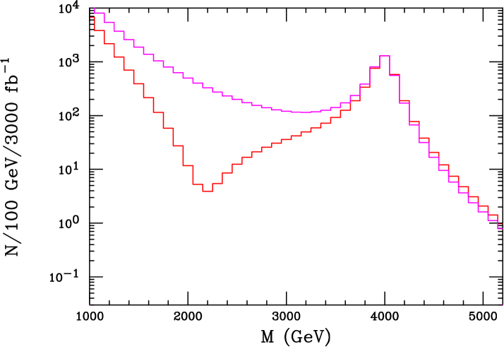
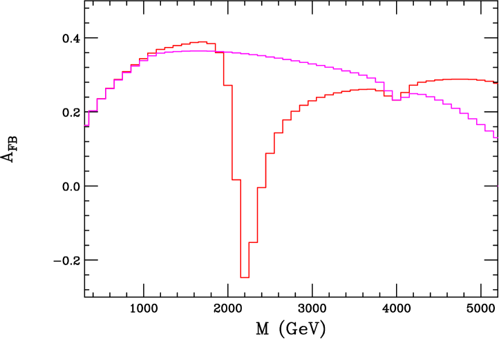
Figure 3: A comparison of the lepton pair invariant mass spectrum and forward-backward lepton asymmetry for the production of a 4 TeV KK resonance for the two choices of $D$. The red(magenta) histograms are for the case $D=0(\pi R)$.

For either $D$ choice the excitation curve and $A_{FB}$ appear to be qualitatively different than that which one obtains for typical $Z^{\prime}$ models[8] as is shown in Figs. 4 and 5. None of the dozen $Z^{\prime}$ models produces resonance structures that appear anything like that seen for the KK case. The resonance structure for the KK case is significantly wider and has a larger peak cross section than does the typical $Z^{\prime}$ model where the strong destructive interference below the resonance is absent. (We remember however that the height and width of the $Z^{\prime}$ or KK resonance also depends on the set of allowed decay modes.) In addition, the dip in the value of $A_{FB}$ occurs much closer to the resonance region for the typical $Z^{\prime}$ model than it does in the KK case. Clearly, while the KK resonance does not look like one of the usual $Z^{\prime}$’s, we certainly could not claim, based on these figures, that some $Z^{\prime}$ model with which we are not familiar cannot mimic either KK case. In fact, from the figures, one can more easily imagine a $Z^{\prime}$ with stronger than typical couplings leading to an excitation structure similar to the $D=\pi R$ KK case, i.e., it seems more likely that the case of $D=\pi R$ can be mimicked by a (strongly coupled) $Z^{\prime}$ than does the $D=0$ case.

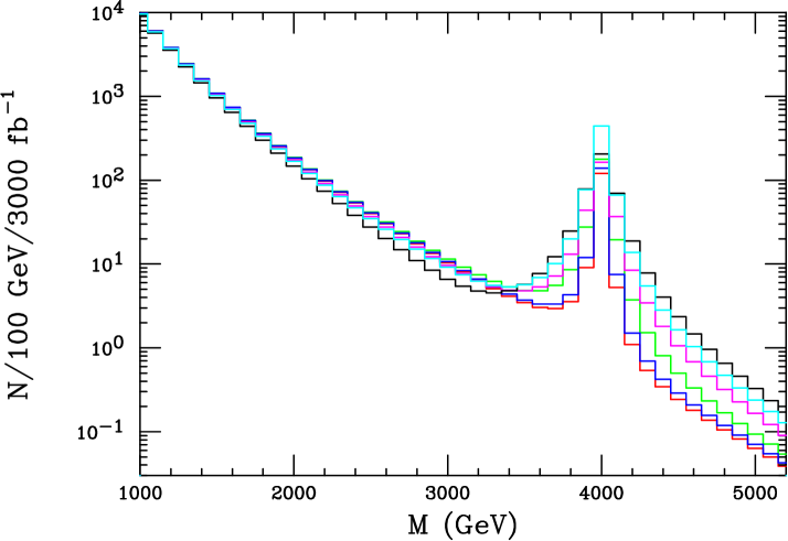
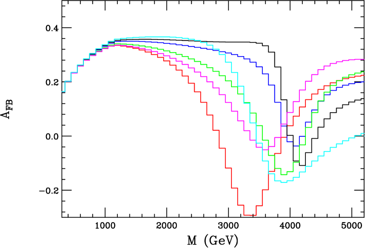
Figure 4: Same as in the previous pair of figures but now for a number of $Z^{\prime}$ models. The red(green, blue, magenta, cyan, black) histograms correspond to $E_{6}$ model $\psi(\chi,~{}\eta)$, the Left Right Symmetric Model with $\kappa=g_{R}/g_{L}=1$, the Alternative Left Right Model and the Sequential Standard Model, respectively. For descriptions of these models and original references see Ref.[8].

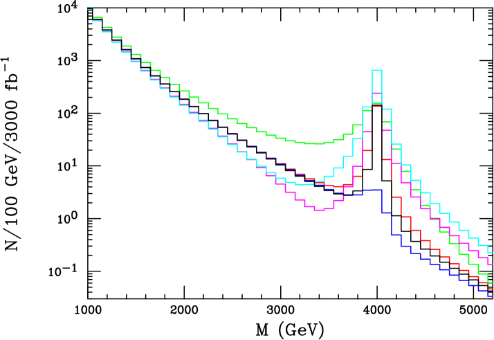
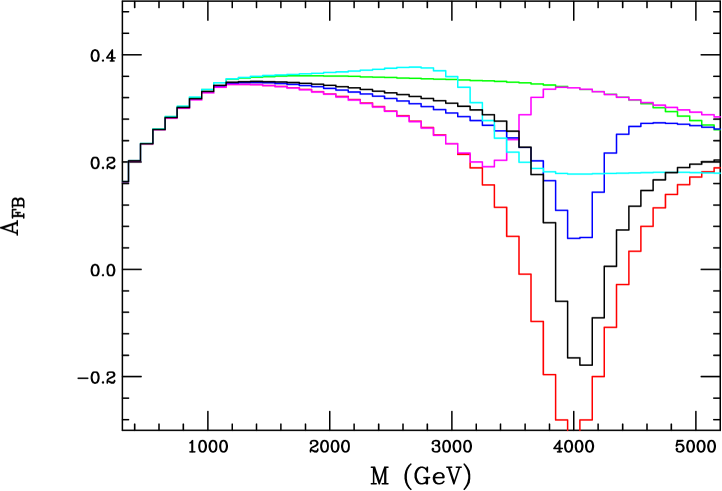
Figure 5: Same as in the previous pair of figures but now for a further set of $Z^{\prime}$ models. The red(green, blue, magenta, cyan, black) histograms correspond to $E_{6}$ model $I$, the Un-unified Model with $s_{\phi}=0.6$, the Foot-Hernandez model, the model of Kuo et al., a $Z^{\prime}$ coupling proportional to hypercharge and $E_{6}$ model $\eta$ with gauge kinetic mixing parameter $\delta=0.25$, respectively. For descriptions of these models and original references see Ref.[8].

In order to quantify the differences between the KK and $Z^{\prime}$ scenarios we must choose observables that have reasonable statistical power associated with them and do not explicitly depend on any assumptions about how the KK or $Z^{\prime}$ may decay, e.g., if the resonance has non-SM decays such as into supersymmetric final states. Consider the $D=0$ case; given the $100-3000$ $fb^{-1}$ luminosity of the LHC and its upgrade, the invariant mass distribution will only be useful as an observable for lepton pair masses above the $Z$ pole and below $\sim 2.5$ TeV and as well as near the KK/$Z^{\prime}$ resonance. Outside these regions there is either no sensitivity to new physics or the event rate is just too low to make decent measurements. As we noted above the resonance region we cannot use fairly if we assume that all of the decays of the resonance are a priori unknown. Once we are safely beyond the peak region the cross section is quite small yielding too poor a set of statistics to be valuable.

Since the statistics required to determine $A_{FB}$ is significantly higher for a fixed value of the invariant mass than it is for the mass distribution itself (because angular distributions now need to be measured as well), its range of usefulness as a differentiating observable is more restricted. Perhaps below $\sim 1.5$ TeV in dilepton invariant mass sufficient statistics will be available to allow $A_{FB}$ to be useful. However, one might imagine that $A_{FB}$ may also be helpful very near the peak region since we know that for the case of a $Z^{\prime}$, $A_{FB}$ is approximately independent of what modes the resonance may decay into, unlike the cross section. Naively, we would expect the inclusion of input from $A_{FB}$ data on the peak to improve the results obtained below. However, it has been shown in our earlier work[10] that even near the apparent KK pole, $A_{FB}$ depends on the relative total widths of the individual $\gamma$ and $Z$ KK excitations, which is model sensitive. In the analysis presented below we will ignore any additional guidance that may arise from considering the values of $A_{FB}$ at lepton pair masses below $\sim 1.5$ TeV and examine only the invariant mass distribution, i.e., the possible additional information obtainable from $A_{FB}$ will be ignored in the present analysis and will be left for later study.

Turning to our analysis, for $M_{c}=4(5,~{}6)$ TeV we begin by generating cross section ‘data’ corresponding to dilepton masses in the range 250-1850(2150, 2450) GeV in 100 GeV bins for both the $D=0$ and $\pi R$ cases. To go any lower in mass would not be very useful as we are then dominated by either the $Z$ peak or the photon pole. For larger masses the cross section is either too small in the $D=0$ case or is dominated by the heavy resonance as discussed above. Next we try to fit these cross section distributions by making the assumption that the data is generated by a single $Z^{\prime}$. For simplicity, we restrict our attention to the class of $Z^{\prime}$ models with generation-independent couplings and where the $Z^{\prime}$ has associated with it a new gauge group generator that commutes with weak isospin. These conditions are satisfied, e.g., by GUT-inspired $Z^{\prime}$ models as well as by many others in the literature[8]. If these constraints hold then the $Z^{\prime}$ couplings to all SM fermions can be described by only 5 independent parameters: the couplings to the left-handed quark and lepton doublets and the corresponding ones to the right-handed quarks and leptons. We then vary all of these couplings independently in order to obtain the best $\chi^{2}/df$ fit to the dilepton mass distribution and obtain the relevant probability/confidence level(CL) using statistical errors only. Systematic errors arising from, e.g., parton distribution function uncertainties will be ignored. In practice this is a fine-grained scan over a rather large volume of the 5-d parameter space examining more than $10^{10}$ coupling combinations for each of the cases we consider to obtain the best probability. In performing this fit it is assumed that the apparent $Z^{\prime}$ mass is the same as that of the produced KK state which will be directly measured. In this approach, the overall normalization of the cross section is determined at the $Z$-pole which is outside of the fit region and is governed solely by SM physics.

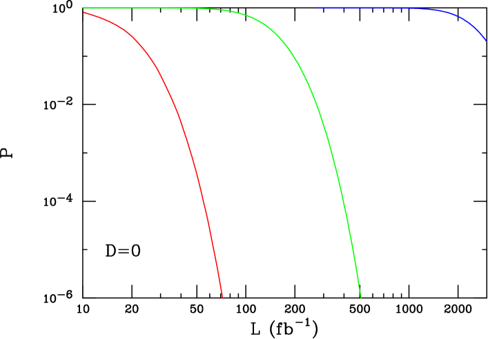
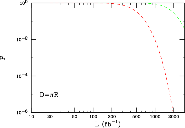
Figure 6: Probability associated with the best $Z^{\prime}$ fit hypothesis as a function of the LHC integrated luminosity for the cases $D=0$ and $D=\pi R$. From left to right the curves correspond to the choice $M_{c}=4$, 5 and 6 TeV, respectively.

The results of performing these fits for different values of $M_{c}$ and the two choices $D=0,\pi R$ are shown in Fig. 6. Explicitly, these show the best fit probability for the $Z^{\prime}$ hypothesis to the KK generated data. For example, taking the case $D=0$ with $M_{c}=4$ TeV we see that with an integrated luminosity of order 60 $fb^{-1}$ the best fit probability is near a few $\times 10^{-5}$. For such low probabilities we can certainly claim that the KK generated ‘data’ is not well fit by the $Z^{\prime}$ hypothesis. As the mass of the KK state increases the size of the shift in the production cross section from the SM expectation is reduced and greater statistics are needed to obtain the same probability level. For $M_{c}=5$ TeV we see that an integrated luminosity of order 400 $fb^{-1}$ is required to get to the same level of rejection of the $Z^{\prime}$ hypothesis as above. Similarly, for $M_{c}=6$ TeV extremely high luminosities of order 7-8 $ab^{-1}$ would be required to get to this level of probability, which is most likely a factor of two or so beyond even that expected for the LHC upgrades unless combined data from both detectors was used.

For the $D=\pi R$ case we see the situation is somewhat different in that the level of ‘confusion’ between the KK and $Z^{\prime}$ is potentially greater. This is what we might have expected based on our discussion above. Even for the case $M_{c}=4$ TeV we see that only at very high integrated luminosities of order $\sim 1.5~{}ab^{-1}$ can the KK and $Z^{\prime}$ scenarios be distinguished at the level discussed above. With $M_{c}=5$ TeV, approximately 6 $ab^{-1}$ would be required to reach the same rejection level. For larger KK masses this separation becomes essentially impossible at the LHC.

3 What Can the LC Tell Us?

The analysis for the LC is somewhat different than at the LHC. No actual resonances are produced but deviations from SM cross sections and asymmetries are observed due the $s$-channel exchanges of the $Z^{\prime}$ or KK gauge boson towers. Though subtle these two sets of deviations are not identical and our hope here is to use the precision measurement capability of a LC to distinguish them. We will assume that data is taken at a single value of $\sqrt{s}$ so that the mass of the KK or $Z^{\prime}$ resonance obtained from the LHC must be used as an input to the analysis as presented here. Without such an input the analysis below can still be performed provided data from at least two distinct values of $\sqrt{s}$ are used as input[12]. In that case $M_{c}$ becomes an additional fit parameter to be determined by the analysis from the $\sqrt{s}$ dependence of the deviations from the SM expectations. While this more general situation is certainly very interesting it is beyond the scope of the present analysis.

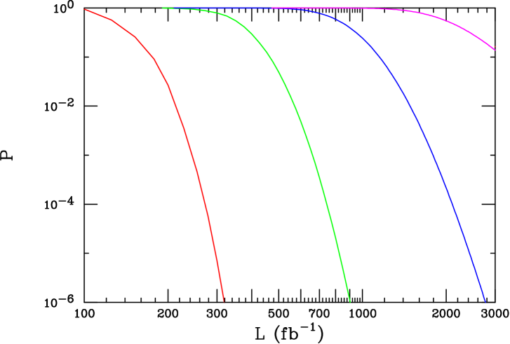
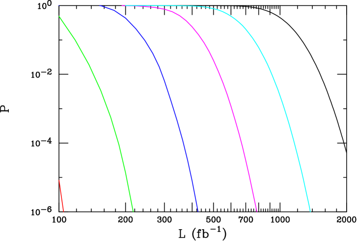
Figure 7: Same as the previous figure but now for a 500(1000) GeV LC in the top(bottom) panel. The $D=0$ and $D=\pi R$ cases are identical here. From left to right the curves are for the cases $M_{c}=4,5,6,..$ TeV etc. The value of $M_{c}$ is assumed to be determined at the LHC.

Consider the general process $e^{+}e^{-}\rightarrow f\bar{f}$; assuming KK states are actually present with a fixed $M_{c}$ as above, we generate ‘data’ for both the differential cross section as well as the Left-Right polarization asymmetry, $A_{LR}$, including the effects of ISR, as functions of the scattering angle, i.e., $\cos\theta$, in 20 (essentially) equal sized bins. The electron beam is assumed to be $80\%$ polarized and angular acceptance cuts are applied. Our other detailed assumptions in performing this analysis are the same as those employed in earlier studies and can be found in Ref.[13]. We then attempt to fit this ‘data’ making the assumption that the deviations from the SM are due to a single $Z^{\prime}$. For simplicity, here we will concentrate on the processes $e^{+}e^{-}\rightarrow\mu^{+}\mu^{-},\tau^{+}\tau^{-}$ as only the two leptonic couplings are involved in performing any fits. In this case the $D=0$ and $D=\pi R$ scenarios lead to identical results for the shifts in all observables at the LC, an advantage over the LHC case. Adding new final states, such as $b\bar{b}$ or $c\bar{c}$, may lead to potential improvements although additional fit parameters now must be introduced and the $D=0$ and $D=\pi R$ predictions would then again be distinct as at the LHC. To be specific, we consider two cases for the LC center of mass energy: $\sqrt{s}=0.5$ and 1 TeV. We remind the reader that while these two leptonic couplings are adequate to describe the effects of $Z^{\prime}$ exchange the description fails in the case of KK states since towers of both the $\gamma$ and $Z$ are being exchanged; this naturally requires three couplings in general since the photon tower has only vector couplings to SM fermions.

As before in the LHC case we next vary the two assumed $Z^{\prime}$ couplings to leptons to obtain the best $\chi^{2}/df$ for the fit which then leads to the probabilities shown in Fig. 7. For the case of a $\sqrt{s}$=500 GeV LC, we see that an integrated luminosity of 300 $fb^{-1}$ is roughly equivalent to 60 $fb^{-1}$ at the LHC for the case of $M_{c}=4$ TeV assuming $D=0$. For larger values of $M_{c}$ the 500 GeV LC does slightly better at KK/$Z^{\prime}$ discrimination than the LHC: 800(2200) $fb^{-1}$ at the LC equivalent is found to be roughly equivalent to 400(7500) $fb^{-1}$ at the LHC assuming $M_{c}=5(6)$ TeV. Since the $D=0$ and $\pi R$ cases are identical at the LC a further advantage is obtained there as noted earlier. Once the LC energy increases to 1 TeV the LC is seen to be superior in model separation but the analysis still relies upon the LHC to input the value of $M_{c}$ in the fits. The lower panel in Fig. 7 shows results for values of $M_{c}$ beyond the range of 7-8 TeV which is directly observable at the LHC. This would seem to imply that by extending the present analysis to include input from at least two values of $\sqrt{s}$ we may be able to extend the KK/$Z^{\prime}$ separation out to very large masses at the LC.

As a final point one may wonder about the reverse problem, i.e., if the heavy resonance observed at the LHC is a $Z^{\prime}$, how do we rule out the possibility of it being a KK state? From performing the analysis discussed above at both the LHC and LC we would know that the resonance couplings would be consistent with being a $Z^{\prime}$ and not a KK state (at least not one of the type we have considered here). In particular, given the mass of the state from the LHC, the LC with its excellent $b$ and $c$ tagging capabilities would be able to provide a good fit to the various flavor couplings of the $Z^{\prime}$ in addition to the leptonic ones considered here. Thus it seems reasonably straightforward that if a $Z^{\prime}$ is discovered, given the present analysis and its extensions to other final states at the LC, it will be quite clear that it is indeed a $Z^{\prime}$ and not a KK state.

4 Summary and Conclusion

New physics signatures arising from different sources may be confused when first observed at future colliders. Thus it is important to examine how various scenarios may be differentiated given the availability of only limited information. In this analysis we have performed a comparison of the capabilities of the LHC and LC to differentiate new physics associated with KK and $Z^{\prime}$ excitations. In the present study the LC reach was found to be somewhat superior to that of the LHC but the LC analysis depended upon the LHC determination of the resonance mass as an input. It would be useful to perform both of these studies at the level of fast MC to verify the results obtained here, including systematic effects as well as the input of $A_{FB}$ data at the LHC and Bhabha scattering data at the LC. The analysis as presented here can also be extended to other scenarios which will be considered elsewhere.

As a final point one may wonder about the reverse problem, i.e., if the heavy resonance observed at the LHC is a $Z^{\prime}$, how do we rule out the possibility of it being a KK state? From performing the analysis discussed above at both the LHC and LC we would know that the couplings would be consistent with being a $Z^{\prime}$ and not

Acknowledgements

The author would like to thank G. Azuelos, J. L. Hewett, and G. Polesello for discussions related to this analysis.

References

- [1] See, for example, I. Antoniadis, Phys. Lett. B246, 377 (1990); I. Antoniadis, C. Munoz and M. Quiros, Nucl. Phys. B397, 515 (1993); I. Antoniadis and K. Benalki, Phys. Lett. B326, 69 (1994)and Int. J. Mod. Phys. A15, 4237 (2000); I. Antoniadis, K. Benalki and M. Quiros, Phys. Lett. B331, 313 (1994).
- [2] M. Carena, E. Ponton, T. M. Tait and C. E. Wagner, arXiv:hep-ph/0212307; M. Carena, T. M. Tait and C. E. Wagner, Acta Phys. Polon. B 33, 2355 (2002) [arXiv:hep-ph/0207056]; H. Davoudiasl, J. L. Hewett and T. G. Rizzo, arXiv:hep-ph/0212279.
- [3] T. Appelquist, H. C. Cheng and B. A. Dobrescu, Phys. Rev. D 64, 035002 (2001) [arXiv:hep-ph/0012100]; H. C. Cheng, K. T. Matchev and M. Schmaltz, Phys. Rev. D 66, 056006 (2002) [arXiv:hep-ph/0205314] and Phys. Rev. D 66, 036005 (2002) [arXiv:hep-ph/0204342]; T. G. Rizzo, Phys. Rev. D 64, 095010 (2001) [arXiv:hep-ph/0106336].
- [4] See, for example, T.G. Rizzo and J.D. Wells, Phys. Rev. D61, 016007 (2000); P. Nath and M. Yamaguchi, Phys. Rev. D60, 116006 (1999); M. Masip and A. Pomarol, Phys. Rev. D60, 096005 (1999); L. Hall and C. Kolda, Phys. Lett. B459, 213 (1999); R. Casalbuoni, S. DeCurtis, D. Dominici and R. Gatto, Phys. Lett. B462, 48 (1999); A. Strumia, Phys. Lett. B466, 107 (1999); F. Cornet, M. Relano and J. Rico, Phys. Rev. D61, 037701 (2000); C.D. Carone, Phys. Rev. D61, 015008 (2000).
- [5] T.G. Rizzo, Phys. Rev. D61, 055005 (2000) and Phys. Rev. D64, 015003 (2001).
- [6] L. Randall and R. Sundrum, Phys. Rev. Lett. 83, 3370 (1999) [arXiv:hep-ph/9905221].
- [7] For an overview of the Randall-Sundrum model phenomenology, see H. Davoudiasl, J.L. Hewett and T.G. Rizzo, Phys. Rev. Lett. 84, 2080 (2000); Phys. Lett. B493, 135 (2000); and Phys. Rev. D63, 075004 (2001).
- [8] For a review of new gauge boson physics at colliders and details of the various models, see J.L. Hewett and T.G. Rizzo, Phys. Rep. 183, 193 (1989); M. Cvetic and S. Godfrey, in Electroweak Symmetry Breaking and Beyond the Standard Model, ed. T. Barklow et al., (World Scientific, Singapore, 1995), hep-ph/9504216; T.G. Rizzo in New Directions for High Energy Physics: Snowmass 1996, ed. D.G. Cassel, L. Trindle Gennari and R.H. Siemann, (SLAC, 1997), hep-ph/9612440; A. Leike, Phys. Rep. 317, 143 (1999).
- [9] This is a common feature of the class of models wherein the usual of the SM is the result of a diagonal breaking of a product of two or more ’s. For a discussion of a few of these models, see H. Georgi, E.E. Jenkins, and E.H. Simmons, Phys. Rev. Lett. 62, 2789 (1989) and Nucl. Phys. B331, 541 (1990); V. Barger and T.G. Rizzo, Phys. Rev. D41, 946 (1990); T.G. Rizzo, Int. J. Mod. Phys. A7, 91 (1992); R.S. Chivukula, E.H. Simmons and J. Terning, Phys. Lett. B346, 284 (1995); A. Bagneid, T.K. Kuo, and N. Nakagawa, Int. J. Mod. Phys. A2, 1327 (1987) and Int. J. Mod. Phys. A2, 1351 (1987); D.J. Muller and S. Nandi, Phys. Lett. B383, 345 (1996); X.Li and E. Ma, Phys. Rev. Lett. 47, 1788 (1981) and Phys. Rev. D46, 1905 (1992); E. Malkawi, T.Tait and C.-P. Yuan, Phys. Lett. B385, 304 (1996).
- [10] See, for example, the analysis by G. Azuelos and G. Polesello in, G. Azuelos et al., “The beyond the standard model working group: Summary report,” Proceedings of Workshop on Physics at TeV Colliders, Les Houches, France, 21 May - 1 Jun 2001, arXiv:hep-ph/0204031; T. G. Rizzo, in Proc. of the APS/DPF/DPB Summer Study on the Future of Particle Physics (Snowmass 2001) ed. N. Graf, eConf C010630, P304 (2001) [arXiv:hep-ph/0109179].
- [11] F. Gianotti et al., arXiv:hep-ph/0204087.
- [12] T. G. Rizzo, Phys. Rev. D 55, 5483 (1997) [arXiv:hep-ph/9612304].
- [13] T. G. Rizzo, [arXiv:hep-ph/0303056].