Extrinsic CPT Violation in Neutrino Oscillations in Matter

Abstract

We investigate matter-induced (or extrinsic) CPT violation effects in neutrino oscillations in matter. Especially, we present approximate analytical formulas for the CPT-violating probability differences for three flavor neutrino oscillations in matter with an arbitrary matter density profile. Note that we assume that the CPT invariance theorem holds, which means that the CPT violation effects arise entirely because of the presence of matter. As special cases of matter density profiles, we consider constant and step-function matter density profiles, which are relevant for neutrino oscillation physics in accelerator and reactor long baseline experiments as well as neutrino factories. Finally, the implications of extrinsic CPT violation on neutrino oscillations in matter for several past, present, and future long baseline experiments are estimated.

I Introduction

Recently, several studies on CPT violation Coleman:1997xq ; Coleman:1998ti ; Barger:2000iv ; Murayama:2000hm ; Banuls:2001zn ; Barenboim:2001ac ; Barenboim:2002rv ; Barenboim:2002hx ; Barenboim:2002tz ; Barenboim:2002ah ; Pakvasa:2001yw ; Xing:2001ys ; Skadhauge:2001kk ; Bilenky:2001ka ; Ohlsson:2002ne ; Bahcall:2002ia ; Strumia:2002fw ; Mocioiu:2002pz ; DeGouvea:2002xp have been performed in order to incorporate the so-called LSND anomaly Athanassopoulos:1996jb ; Athanassopoulos:1998pv ; Aguilar:2001ty within the description of standard three flavor neutrino oscillations. However, this requires a new mass squared difference different from the ones coming from atmospheric Fukuda:1998mi ; Fukuda:1998ah ; Fukuda:2000np ; Shiozawa:2002 and solar Fukuda:2001nj ; Fukuda:2001nk ; Smy:2001wf ; Fukuda:2002pe ; Smy:2002 ; Ahmad:2001an ; Ahmad:2002jz ; Ahmad:2002ka ; Hallin:2002 neutrinos, which means that one would need to have three mass squared differences instead of two – a scenario, which is not consistent with ordinary models of three flavor neutrino oscillations. Therefore, in most of the studies on CPT violation Murayama:2000hm ; Barenboim:2001ac ; Barenboim:2002rv ; Barenboim:2002hx ; Barenboim:2002ah ; Skadhauge:2001kk ; Bilenky:2001ka ; Ohlsson:2002ne ; Bahcall:2002ia ; Strumia:2002fw , different mass squared differences and mixing parameters are introduced phenomenologically by hand for neutrinos and antineutrinos. This results, in the three neutrino flavor picture, in two mass squared differences and four mixing parameters for neutrinos and the same for antineutrinos, i.e., in total, four mass squared differences and eight mixing parameters. Thus, it is possible to have a different mass squared difference describing the results of the LSND experiment other than the ones describing atmospheric and solar neutrino data. It should be noted that the results of the LSND experiment will be further tested by the MiniBooNE experiment miniboone , which started running in September 2002. Furthermore, it should be mentioned that the standard way of incorporating the LSND data is to introduce sterile neutrinos, and therefore, the introduction of fundamental CPT violation, sometimes also called genuine CPT violation, serves as an alternative description to sterile neutrinos. However, neutrino oscillations between pure sterile flavors and active and sterile flavors have, in principle, been excluded by the SNO experiment Ahmad:2002jz ; Ahmad:2002ka ; Bahcall:2002hv .

In CPT violation studies, the CPT invariance theorem Luders:1954 ; Pauli:1955 ; Bell:1955 , a milestone of local quantum field theory, obviously does not hold, and in addition, fundamental properties such as Lorentz invariance and locality may also be violated. However, the ${\rm SU(3)\times SU(2)\times U(1)}$ Standard Model (SM) of elementary particle physics, for which the CPT theorem is valid, is in very good agreement with all existing experimental data. Therefore, fundamental CPT violation is connected to physics beyond the SM such as string theory or models including extra dimensions, in which CPT invariance could be violated.

The recent and the first results of the KamLAND experiment Eguchi:2002dm , which is a reactor long baseline neutrino oscillation experiment measuring the $\bar{\nu}_{e}$ flux from distant nuclear reactors in Japan and South Korea, strongly favor the large mixing angle (LMA) solution region for solar neutrino oscillations and the solar neutrino problem Bahcall:2002ij . Therefore, they indicate that there is no need for fundamental CPT violation, i.e., having different mass squared differences for solar neutrinos and reactor antineutrinos. Thus, solar neutrino data and KamLAND data can be simultaneously and consistently accommodated with the same mass squared difference.

In this paper, we investigate matter-induced (or extrinsic) CPT violation effects in neutrino oscillations in matter. In a previous paper Akhmedov:2001kd , the interplay between fundamental and matter-induced T violation effects has been discussed. In the case of CPT violation effects, there exists no fundamental (or intrinsic) CPT violation effects if we assume that the CPT theorem holds. This means that the matter-induced CPT violation is a pure effect of the simple fact that ordinary matter consists of unequal numbers of particles and antiparticles. Matter-induced CPT violation, sometimes also called fake CPT violation, have been studied and illustrated in some papers Bernabeu:1999gr ; Banuls:2001zn ; Bernabeu:2001xn ; Bernabeu:2001jb ; Xing:2001ys ; Bernabeu:2002tj , in which numerical calculations of CPT-violating asymmetries between survival probabilities for neutrinos and antineutrinos in different scenarios of atmospheric and long-baseline neutrino oscillation experiments have been presented. Here we will try to perform a much more systematic study.

The paper is organized as follows. In Sec. II, we discuss the general formalism and properties of CPT violation in vacuum and in matter. In particular, we derive approximate analytical formulas for all CPT-violating probability differences for three flavor neutrino oscillations in matter with an arbitrary matter density profile. The derivations are performed using first order perturbation theory in the small leptonic mixing angle $\theta_{13}$ for the neutrino and antineutrino evolution operators as well as the fact that $\Delta m_{21}^{2}\ll\Delta m_{31}^{2}\simeq\Delta m_{32}^{2}$, i.e., the solar mass squared difference is some orders of magnitude smaller than the atmospheric mass squared difference. At the end of this section, we consider two different explicit examples of matter density profiles. These are constant and step-function matter density profiles. In both cases, we present the first order perturbation theory formulas for the CPT probability differences as well as the useful corresponding low-energy region formulas. Next, in Sec. III, we discuss the implications for long baseline neutrino oscillation experiments and potential neutrino factory setups as well as solar and atmospheric neutrinos. We illuminate the discussion with several tables and plots of the CPT probability differences. Then, in Sec. IV, we present a summary of the obtained results as well as our conclusions. Finally, in App. A, we give details of the general analytical derivation of the evolution operators for neutrinos and antineutrinos.

II General Formalism and CPT-Violating Probability Differences

II.1 Neutrino Oscillation Transition Probabilities and CP, T, and CPT Violation

Let us by $P(\nu_{\alpha}\to\nu_{\beta}$) denote the transition probability from a neutrino flavor $\alpha$ to a neutrino flavor $\beta$, and similarly, for antineutrino flavors. Then, the CP, T, and CPT (-violating) probability differences are given by

$$\Delta P_{\alpha\beta}^{\rm CP} \equiv P(\nu_{\alpha}\to\nu_{\beta})-P(\bar{\nu}_{\alpha}\to\bar{\nu}_{\beta}),$$ (1)

$$\Delta P_{\alpha\beta}^{\rm T} \equiv P(\nu_{\alpha}\to\nu_{\beta})-P(\nu_{\beta}\to\nu_{\alpha}),$$ (2)

$$\Delta P_{\alpha\beta}^{\rm CPT} \equiv P(\nu_{\alpha}\to\nu_{\beta})-P(\bar{\nu}_{\beta}\to\bar{\nu}_{\alpha}),$$ (3)

where $\alpha,\beta=e,\mu,\tau,\ldots$. The CP and T probability differences have previously been extensively studied in the literature Arafune:1997hd ; Minakata:1998bf ; Minakata:1997td ; Schubert:1999ky ; Dick:1999ed ; Donini:1999jc ; Cervera:2000kp ; Minakata:2000ee ; Barger:2000ax ; Fishbane:2000kw ; Gonzalez-Garcia:2001mp ; Minakata:2001qm ; Minakata:2002qe ; Kimura:2002wd ; Yokomakura:2002av ; Ota:2002fu ; Kuo:1987km ; Krastev:1988yu ; Toshev:1989vz ; Toshev:1991ku ; Arafune:1997bt ; Koike:1997dh ; Bilenky:1998dd ; Barger:1999hi ; Koike:1999hf ; Yasuda:1999uv ; Sato:1999wt ; Koike:1999tb ; Harrison:1999df ; Naumov:1992rh ; Naumov:1992ju ; Yokomakura:2000sv ; Parke:2000hu ; Koike:2000jf ; Miura:2001pi ; Akhmedov:2001kd ; Miura:2001pi2 ; Rubbia:2001pk ; Xing:2001cx ; Ota:2001cz ; Ohlsson:2001ps ; Bueno:2001jd ; Sato:2001dt ; Akhmedov:2002za ; Minakata:2002qi ; Huber:2002uy ; Leung:2003cb . In this paper, we will study in detail the CPT probability differences. Let us first dicuss some general properties of the CPT probability differences. In general, i.e., both in vacuum and in matter, it follows from conservation of probability that

$$\sum_{\alpha=e,\mu,\tau,\ldots}P(\nu_{\alpha}\to\nu_{\beta}) = 1,\quad\beta=e,\mu,\tau,\ldots,$$ (4)

$$\sum_{\beta=e,\mu,\tau,\ldots}P(\nu_{\alpha}\to\nu_{\beta}) = 1,\quad\alpha=e,\mu,\tau,\ldots.\$$ (5)

In words, the sum of the transition probabilities of a given neutrino (antineutrino) flavor into neutrinos (antineutrinos) of all possible flavors is, of course, equal to one, i.e., the probability is conserved. Using the definitions of the CPT probability differences, Eqs. (4) and (5) can be re-written as

$$\sum_{\alpha=e,\mu,\tau,\ldots}\Delta P_{\alpha\beta}^{\rm CPT} = 0,\quad\beta=e,\mu,\tau,\ldots,$$ (6)

$$\sum_{\beta=e,\mu,\tau,\ldots}\Delta P_{\alpha\beta}^{\rm CPT} = 0,\quad\alpha=e,\mu,\tau,\ldots.$$ (7)

Note that not all of these equations are linearly independent. For example, for three neutrino flavors, Eqs. (6) and (7) can be written as the following system of equations

$$\Delta P_{ee}^{\rm CPT}+\Delta P_{e\mu}^{\rm CPT}+\Delta P_{e\tau}^{\rm CPT} = 0,$$ (8)

$$\Delta P_{\mu e}^{\rm CPT}+\Delta P_{\mu\mu}^{\rm CPT}+\Delta P_{\mu\tau}^{\rm CPT} = 0,$$ (9)

$$\Delta P_{\tau e}^{\rm CPT}+\Delta P_{\tau\mu}^{\rm CPT}+\Delta P_{\tau\tau}^{\rm CPT} = 0,$$ (10)

$$\Delta P_{ee}^{\rm CPT}+\Delta P_{\mu e}^{\rm CPT}+\Delta P_{\tau e}^{\rm CPT} = 0,$$ (11)

$$\Delta P_{e\mu}^{\rm CPT}+\Delta P_{\mu\mu}^{\rm CPT}+\Delta P_{\tau\mu}^{\rm CPT} = 0,$$ (12)

$$\Delta P_{e\tau}^{\rm CPT}+\Delta P_{\mu\tau}^{\rm CPT}+\Delta P_{\tau\tau}^{\rm CPT} = 0.$$ (13)

Hence, there are nine CPT probability differences for neutrinos and six equations relating these CPT probability differences. The rank of the corresponding system matrix for the above system of equations is five, which means that only five of the six equations are linearly independent. Thus, five out of the nine CPT probability differences can be expressed in terms of the other four, i.e., there are, in fact, only four CPT probability differences. Choosing, e.g., $\Delta P_{ee}^{\rm CPT}$, $\Delta P_{e\mu}^{\rm CPT}$, $\Delta P_{\mu e}^{\rm CPT}$, and $\Delta P_{\mu\mu}^{\rm CPT}$ as the known CPT probability differences, the other five can be expressed as

$$\Delta P_{e\tau}^{\rm CPT} = -\Delta P_{ee}^{\rm CPT}-\Delta P_{e\mu}^{\rm CPT},$$ (14)

$$\Delta P_{\mu\tau}^{\rm CPT} = -\Delta P_{\mu e}^{\rm CPT}-\Delta P_{\mu\mu}^{\rm CPT},$$ (15)

$$\Delta P_{\tau e}^{\rm CPT} = -\Delta P_{ee}^{\rm CPT}-\Delta P_{\mu e}^{\rm CPT},$$ (16)

$$\Delta P_{\tau\mu}^{\rm CPT} = -\Delta P_{e\mu}^{\rm CPT}-\Delta P_{\mu\mu}^{\rm CPT},$$ (17)

$$\Delta P_{\tau\tau}^{\rm CPT} = \Delta P_{ee}^{\rm CPT}+\Delta P_{e\mu}^{\rm CPT}+\Delta P_{\mu e}^{\rm CPT}+\Delta P_{\mu\mu}^{\rm CPT}.$$ (18)

Furthermore, the CPT probability differences for neutrinos are related to the ones for antineutrinos by

$$\Delta P_{\alpha\beta}^{\rm CPT} = P(\nu_{\alpha}\to\nu_{\beta})-P(\bar{\nu}_{\beta}\to\bar{\nu}_{\alpha})$$ (19)

$$= -(P(\bar{\nu}_{\beta}\to\bar{\nu}_{\alpha})-P(\nu_{\alpha}\to\nu_{\beta}))=-\Delta P_{\bar{\beta}\bar{\alpha}}^{\rm CPT},$$

where $\alpha,\beta=e,\mu,\tau,\ldots$. Thus, the CPT probability differences for antineutrinos do not give any further information.

For completeness, we shall also briefly consider the case of two neutrino flavors. In this case, we have

$$\Delta P_{ee}^{\rm CPT}+\Delta P_{e\mu}^{\rm CPT} = 0,$$ (20)

$$\Delta P_{\mu e}^{\rm CPT}+\Delta P_{\mu\mu}^{\rm CPT} = 0,$$ (21)

$$\Delta P_{ee}^{\rm CPT}+\Delta P_{\mu e}^{\rm CPT} = 0,$$ (22)

$$\Delta P_{e\mu}^{\rm CPT}+\Delta P_{\mu\mu}^{\rm CPT} = 0$$ (23)

from which one immediately obtains

$$\Delta P_{ee}^{\rm CPT}=\Delta P_{\mu\mu}^{\rm CPT}=-\Delta P_{e\mu}^{\rm CPT}=-\Delta P_{\mu e}^{\rm CPT}.$$ (24)

Thus, for two neutrino flavors there is only one linearly independent CPT probability difference, which we, e.g., can choose as $\Delta P_{ee}^{\rm CPT}$.

Generally, for the T probability differences, we have Krastev:1988yu ; Akhmedov:2001kd

$$\Delta P_{ee}^{\rm T}=\Delta P_{\mu\mu}^{\rm T}=\Delta P_{\tau\tau}^{\rm T}=0,$$ (25)

$$\Delta P_{e\mu}^{\rm T}=\Delta P_{\mu\tau}^{\rm T}=\Delta P_{\tau e}^{\rm T}=-\Delta P_{\mu e}^{\rm T}=-\Delta P_{\tau\mu}^{\rm T}=-\Delta P_{e\tau}^{\rm T}$$ (26)

for three neutrino flavors and

$$\Delta P_{ee}^{\rm T}=\Delta P_{e\mu}^{\rm T}=\Delta P_{\mu e}^{\rm T}=\Delta P_{\mu\mu}^{T}=0$$ (27)

for two neutrino flavors. Thus, in the case of three neutrino flavors, there is only one linearly independent T probability difference, whereas in the case of two neutrino flavors, neutrino oscillations are T-invariant irrespective of whether they take place in vacuum or in matter.

Using the definitions (1) - (3), one immediately observes that the CP probability differences are directly related to the T and CPT probability differences by the following formulas

$$\Delta P_{\alpha\beta}^{\rm CP}+\Delta P_{\bar{\alpha}\bar{\beta}}^{\rm T}=\Delta P_{\alpha\beta}^{\rm CPT}\quad\mbox{and}\quad\Delta P_{\bar{\alpha}\bar{\beta}}^{\rm CP}+\Delta P_{\alpha\beta}^{\rm T}=\Delta P_{\bar{\alpha}\bar{\beta}}^{\rm CPT}.$$ (28)

In vacuum, where CPT invariance holds, one has $\Delta P_{\alpha\beta}^{\rm CPT}=\Delta P_{\bar{\alpha}\bar{\beta}}^{\rm CPT}=0$, which means that $\Delta P_{\alpha\beta}^{\rm CP}=-\Delta P_{\bar{\alpha}\bar{\beta}}^{\rm T}$ and $\Delta P_{\bar{\alpha}\bar{\beta}}^{\rm CP}=-\Delta P_{\alpha\beta}^{\rm T}$. Furthermore, using again the definition (1), one finds that $\Delta P_{\alpha\beta}^{\rm CP}=-\Delta P_{\bar{\alpha}\bar{\beta}}^{\rm CP}$. Thus, $\Delta P_{\alpha\beta}^{\rm CP}=\Delta P_{\alpha\beta}^{\rm T}$ and $\Delta P_{\bar{\alpha}\bar{\beta}}^{\rm CP}=\Delta P_{\bar{\alpha}\bar{\beta}}^{\rm T}$, i.e., the CP probability differences for neutrinos (antineutrinos) are given by the corresponding T probability differences for neutrinos (antineutrinos). However, in matter, CPT invariance is no longer valid in general, and thus, one has $\Delta P_{\alpha\beta}^{\rm CPT}\neq 0$, which means that we need to know both the T and CPT probability differences in order to determine the CP probability differences. Moreover, in vacuum, it follows in general that $P(\nu_{\alpha}\to\nu_{\beta})=P(\bar{\nu}_{\beta}\to\bar{\nu}_{\alpha})$ and in particular that $P(\nu_{\alpha}\to\nu_{\alpha})=P(\bar{\nu}_{\alpha}\to\bar{\nu}_{\alpha})$, which leads to $\Delta P_{\alpha\alpha}^{\rm CP}=0$. Therefore, CP violation effects cannot occur in disappearance channels ($\nu_{\alpha}\to\nu_{\alpha}$), but only in appearance channels ($\nu_{\alpha}\to\nu_{\beta}$, where $\alpha\neq\beta$) Dick:1999ed , while in matter one has in general $\Delta P_{\alpha\alpha}^{\rm CP}\neq 0$.

In the next subsection, we discuss the Hamiltonians and evolution operators for neutrinos and antineutrinos, which we will use to calculate the CPT probability differences.

II.2 Hamiltonians and Evolution Operators for Neutrinos and Antineutrinos

If neutrinos are massive and mixed, then the neutrino flavor fields $\nu_{\alpha}$, where $\alpha=e,\mu,\tau,\ldots$, are linear combinations of the neutrino mass eigenfields $\nu_{a}$, where $a=1,2,3,\ldots$, i.e.,

$$\nu_{\alpha}=\sum_{a=1}^{n}U_{\alpha a}\nu_{a},\quad\alpha=e,\mu,\tau,\ldots,$$ (29)

where $n$ is the number of neutrino flavors and the $U_{\alpha a}$’s are the matrix elements of the unitary leptonic mixing matrix $U$. Thus, we have the following relation between the neutrino flavor and mass states Bilenky:1978nj ; Bilenky:1987ty

$$|\nu_{\alpha}\rangle=\sum_{a=1}^{n}U_{\alpha a}^{\ast}|\nu_{a}\rangle,\quad\alpha=e,\mu,\tau,\ldots,$$ (30)

where $\nu_{a}$ is the $a$th neutrino mass state for a neutrino with definite 3-momentum ${\bf p}$, energy $E_{a}=\sqrt{m_{a}^{2}+{\bf p}^{2}}\simeq p+\tfrac{m_{a}^{2}}{2p}$ (if $m_{a}\ll p$), and negative helicity. Here $m_{a}$ is the mass of the $a$th neutrino mass eigenstate and $p\equiv|{\bf p}|$. Similarly, for antineutrinos, we have

$$|\bar{\nu}_{\alpha}\rangle=\sum_{a=1}^{n}U_{\alpha a}|\bar{\nu}_{a}\rangle,\quad\alpha=e,\mu,\tau,\ldots.$$ (31)

In the ultra-relativistic approximation, the quantum mechanical time evolution of the neutrino states and the neutrino oscillations are governed by the Schrödinger equation

$${\rm i}\frac{\mathrm{d}}{\mathrm{d}t}|\nu(t)\rangle=\mathscr{H}(t)|\nu(t)\rangle,$$ (32)

where $|\nu(t)\rangle$ is the neutrino vector of state and $\mathscr{H}(t)$ is the time-dependent Hamiltonian of the system, which is different for neutrinos and antineutrinos and its form also depends on in which basis it is given (see App. A for the different expressions of the Hamiltonian). Hence, the neutrino evolution (i.e., the solution to the Schrödinger equation) is given by

$$|\nu(t)\rangle={\rm e}^{-{\rm i}\int_{t_{0}}^{t}\mathscr{H}(t^{\prime})\mathrm{d}t^{\prime}}|\nu(t_{0})\rangle,$$ (33)

where the exponential function is time-ordered. Note that if one assumes that neutrinos are stable and that they are not absorbed in matter, then the Hamiltonian $\mathscr{H}(t)$ is Hermitian. This will be assumed throughout this paper. Furthermore, it is convenient to define the evolution operator (or the evolution matrix) $S(t,t_{0})$ as

$$|\nu(t)\rangle=S(t,t_{0})|\nu(t_{0})\rangle,\quad S(t,t_{0})\equiv{\rm e}^{-{\rm i}\int_{t_{0}}^{t}\mathscr{H}(t^{\prime})\mathrm{d}t^{\prime}},$$ (34)

which has the following obvious properties

$$S(t,t_{0}) = S(t,t_{1})S(t_{1},t_{0}),$$ (35)

$$S(t_{0},t_{0}) = \mathbbm{1},$$ (36)

$$S(t,t_{0})S(t,t_{0})^{\dagger} = \mathbbm{1}.$$ (37)

The last property is the unitarity condition, which follows directly from the hermiticity of the Hamiltonian $\mathscr{H}(t)$.

Neutrinos are produced in weak interaction processes as flavor states $|\nu_{\alpha}\rangle$, where $\alpha=e,\mu,\tau,\ldots$. Between a source, the production point of neutrinos, and a detector, neutrinos evolve as mass eigenstates $|\nu_{a}\rangle$, where $a=1,2,3,\ldots$, i.e., states with definite mass. Thus, if at time $t=t_{0}$ the neutrino vector of state is $|\nu_{\alpha}\rangle\equiv|\nu_{\alpha}(t_{0})\rangle$, then at a time $t$ we have

$$|\nu_{\alpha}(t)\rangle=\sum_{a=1}^{n}\left[S(t,t_{0})\right]_{aa}U_{\alpha a}^{\ast}|\nu_{a}\rangle.$$ (38)

The neutrino oscillation probability amplitude from a neutrino flavor $\alpha$ to a neutrino flavor $\beta$ is defined as

$$A_{\alpha\beta}\equiv\langle\nu_{\beta}|\nu_{\alpha}(t)\rangle=\sum_{a=1}^{n}U_{\beta a}\left[S(t,t_{0})\right]_{aa}U_{\alpha a}^{\ast},\quad\alpha,\beta=e,\mu,\tau,\ldots.$$ (39)

Then, the neutrino oscillation transition probability for $\nu_{\alpha}\to\nu_{\beta}$ is given by

$$P(\nu_{\alpha}\to\nu_{\beta})\equiv|A_{\alpha\beta}|^{2}=\sum_{a=1}^{n}\sum_{b=1}^{n}U_{\alpha a}^{\ast}U_{\beta a}U_{\alpha b}U_{\beta b}^{\ast}\left[S(t,t_{0})\right]_{aa}\left[S(t,t_{0})\right]^{\ast}_{bb},$$ (40)

where $\alpha,\beta=e,\mu,\tau,\ldots$.

The oscillation transition probabilities for antineutrinos are obtained by making the replacements $U_{\alpha a}\to U_{\alpha a}^{\ast}$ and $S(t,t_{0})\to\bar{S}(t,t_{0})$ [i.e., $V(t)\to-V(t)$, where $V(t)$ is the matter potential defined in App. A], which lead to

$$P(\bar{\nu}_{\alpha}\to\bar{\nu}_{\beta}) = \sum_{a=1}^{n}\sum_{b=1}^{n}U_{\alpha a}U_{\beta a}^{\ast}U_{\alpha b}^{\ast}U_{\beta b}\left[\bar{S}(t,t_{0})\right]_{aa}\left[\bar{S}(t,t_{0})\right]^{\ast}_{bb}=\{a\leftrightarrow b\}$$ (41)

$$= \sum_{a=1}^{n}\sum_{b=1}^{n}U_{\alpha a}^{\ast}U_{\beta a}U_{\alpha b}U_{\beta b}^{\ast}\left[\bar{S}(t,t_{0})\right]^{\ast}_{aa}\left[\bar{S}(t,t_{0})\right]_{bb},$$

where $\alpha,\beta=e,\mu,\tau,\ldots$.

In the next subsection, we calculate the CPT probability differences both in vacuum and in matter.

II.3 CPT Probability Differences

In vacuum, the matter potential is zero, i.e., $V(t)=0\;\forall t$, and therefore, the evolution operators for neutrinos and antineutrinos are the same, i.e., $S(t,t_{0})=\bar{S}(t,t_{0})={\rm e}^{-{\rm i}H_{m}L}$, where $H_{m}={\rm diag}\,(E_{1},E_{2},\ldots,E_{n})$ is the free Hamiltonian and $L\simeq t-t_{0}$ is the baseline length. Note that the Hamiltonians in vacuum for neutrinos and antineutrinos are the same, since we have assumed the CPT theorem. Thus, using Eqs. (40) and (41), it directly follows that

$$\Delta P_{\alpha\beta}^{\rm CPT}=P(\nu_{\alpha}\to\nu_{\beta})-P(\bar{\nu}_{\beta}\to\bar{\nu}_{\alpha})=0,$$ (42)

which means that there is simply no (intrinsic) CPT violation in neutrino oscillations in vacuum. Note that this general result holds for any number of neutrino flavors. Furthermore, note that even though there is no intrinsic CPT violation effects in vacuum, there could be intrinsic CP and T violation effects induced by a non-zero CP (or T) violation phase $\delta_{\rm CP}$, which could, if sizeable enough, be measured by very long baseline neutrino oscillation experiments in the future Lindner:2002 .

In matter, the situation is slightly more complicated than in vacuum. However, the technique is the same, i.e., the extrinsic CPT probability differences are given by differences of different matrix elements of the evolution operators for neutrinos and antineutrinos.

The probability amplitude of neutrino flavor transitions are the matrix elements of the evolution operators:

$$A\left(\nu_{\alpha}\rightarrow\nu_{\beta}\right) = \left[S(t,t_{0})\right]_{\beta\alpha}=\left[S_{f}(t,t_{0})\right]_{\beta\alpha},$$ (43)

$$A\left(\bar{\nu}_{\alpha}\rightarrow\bar{\nu}_{\beta}\right) = \left[\bar{S}(t,t_{0})\right]_{\beta\alpha}=\left[\bar{S}_{f}(t,t_{0})\right]_{\beta\alpha}.$$ (44)

Thus, we have the extrinsic CPT probability differences

$$\Delta P_{\alpha\beta}^{CPT}=\left|\left[S_{f}(t,t_{0})\right]_{\beta\alpha}\right|^{2}-\left|\left[\bar{S}_{f}(t,t_{0})\right]_{\alpha\beta}\right|^{2}.$$ (45)

In the case of three neutrino flavors with the evolution operators for neutrinos and antineutrinos as in Eqs. (LABEL:eq:Sf) and (152), respectively, the different $\Delta P_{\alpha\beta}^{\rm CPT}$’s are now easily found, but the expressions are quite unwieldy. The CPT probability difference $\Delta P_{ee}^{\rm CPT}$ to first order in perturbation theory is found to be given by (see App. A for definitions of different quantities)

$$\Delta P_{ee}^{\rm CPT} \simeq |S_{f,11}|^{2}-|\bar{S}_{f,11}|^{2}=|\alpha|^{2}-|\bar{\alpha}|^{2}=|\bar{\beta}|^{2}-|\beta|^{2}$$ (46)

$$= \cos^{2}\Omega+\frac{\sin^{2}\Omega}{4\Omega^{2}}\left(\cos 2\theta_{12}\delta(t-t_{0})-\int_{t_{0}}^{t}V(t^{\prime})\mathrm{d}t^{\prime}\right)^{2}$$

$$- \cos^{2}\bar{\Omega}-\frac{\sin^{2}\bar{\Omega}}{4\bar{\Omega}^{2}}\left(\cos 2\theta_{12}\delta(t-t_{0})+\int_{t_{0}}^{t}V(t^{\prime})\mathrm{d}t^{\prime}\right)^{2}$$

$$= \frac{1}{4}\left(\frac{\sin^{2}\bar{\Omega}}{\bar{\Omega}^{2}}-\frac{\sin^{2}\Omega}{\Omega^{2}}\right)\sin^{2}2\theta_{12}\delta^{2}(t-t_{0})^{2},$$

which is equal to zero in vacuum, in which $V(t)=0\;\forall t$. Note that in the case of T violation all diagonal elements, i.e., $\Delta P_{\alpha\alpha}^{\rm T}$, where $\alpha=e,\mu,\tau$, are trivially equal to zero [cf., Eq. (25)]. This is obviously not the case for CPT violation if matter is present. Similarly, we find

$$\Delta P_{e\mu}^{\rm CPT} \simeq |S_{f,21}|^{2}-|\bar{S}_{f,12}|^{2}=|c_{23}\beta^{\ast}+{\rm i}s_{23}fC|^{2}-|c_{23}\bar{\beta}-{\rm i}s_{23}\bar{f}\bar{A}|^{2}$$ (47)

$$= c_{23}^{2}\left(|\beta|^{2}-|\bar{\beta}|^{2}\right)+s_{23}^{2}\left(|C|^{2}-|\bar{A}|^{2}\right)$$

$$+ {\rm i}s_{23}c_{23}\left(\beta fC-\beta^{\ast}f^{\ast}C^{\ast}+\bar{\beta}^{\ast}\bar{f}\bar{A}-\bar{\beta}\bar{f}^{\ast}\bar{A}^{\ast}\right),$$

$$\Delta P_{e\tau}^{\rm CPT} \simeq |S_{f,31}|^{2}-|\bar{S}_{f,13}|^{2}=|s_{23}\beta^{\ast}-{\rm i}c_{23}fC|^{2}-|-s_{23}\bar{\beta}-{\rm i}c_{23}\bar{f}\bar{A}|^{2}$$ (48)

$$= c_{23}^{2}\left(|C|^{2}-|\bar{A}|^{2}\right)+s_{23}^{2}\left(|\beta|^{2}-|\bar{\beta}|^{2}\right)$$

$$- {\rm i}s_{23}c_{23}\left(\beta fC-\beta^{\ast}f^{\ast}C^{\ast}+\bar{\beta}^{\ast}\bar{f}\bar{A}-\bar{\beta}\bar{f}^{\ast}\bar{A}^{\ast}\right),$$

$$\Delta P_{\mu e}^{\rm CPT} \simeq |S_{f,12}|^{2}-|\bar{S}_{f,21}|^{2}=|c_{23}\beta-{\rm i}s_{23}fA|^{2}-|c_{23}\bar{\beta}^{\ast}+{\rm i}s_{23}\bar{f}\bar{C}|^{2}$$ (49)

$$= c_{23}^{2}\left(|\beta|^{2}-|\bar{\beta}|^{2}\right)+s_{23}^{2}\left(|A|^{2}-|\bar{C}|^{2}\right)$$

$$+ {\rm i}s_{23}c_{23}\left(\beta f^{\ast}A^{\ast}-\beta^{\ast}fA-\bar{\beta}\bar{f}\bar{C}+\bar{\beta}^{\ast}\bar{f}^{\ast}\bar{C}^{\ast}\right),$$

$$\Delta P_{\tau e}^{\rm CPT} \simeq |S_{f,13}|^{2}-|\bar{S}_{f,31}|^{2}=|-s_{23}\beta-{\rm i}c_{23}fA|^{2}-|s_{23}\bar{\beta}^{\ast}-{\rm i}c_{23}\bar{f}\bar{C}|^{2}$$ (50)

$$= c_{23}^{2}\left(|A|^{2}-|\bar{C}|^{2}\right)+s_{23}^{2}\left(|\beta|^{2}-|\bar{\beta}|^{2}\right)$$

$$- {\rm i}s_{23}c_{23}\left(\beta f^{\ast}A^{\ast}-\beta^{\ast}fA-\bar{\beta}\bar{f}\bar{C}+\bar{\beta}^{\ast}\bar{f}^{\ast}\bar{C}^{\ast}\right),$$

$$\Delta P_{\mu\mu}^{\rm CPT} \simeq |S_{f,22}|^{2}-|\bar{S}_{f,22}|^{2}=|c_{23}^{2}\alpha^{\ast}+s_{23}^{2}f-{\rm i}s_{23}c_{23}f(B+D)|^{2}$$ (51)

$$- |c_{23}^{2}\bar{\alpha}^{\ast}+s_{23}^{2}\bar{f}-{\rm i}s_{23}c_{23}\bar{f}(\bar{B}+\bar{D})|^{2}$$

$$= c_{23}^{4}\left(|\alpha|^{2}-|\bar{\alpha}|^{2}\right)-{\rm i}s_{23}c_{23}^{3}\left(\alpha fB-\alpha^{\ast}f^{\ast}B^{\ast}+\alpha fD-\alpha^{\ast}f^{\ast}D^{\ast}\vphantom{\bar{B}^{\ast}}\right.$$

$$\left.\vphantom{\bar{B}^{\ast}}-\bar{\alpha}\bar{f}\bar{B}+\bar{\alpha}^{\ast}\bar{f}^{\ast}\bar{B}^{\ast}-\bar{\alpha}\bar{f}\bar{D}+\bar{\alpha}^{\ast}\bar{f}^{\ast}\bar{D}^{\ast}\right)$$

$$+s_{23}^{2}c_{23}^{2}\left(\alpha f+\alpha^{\ast}f^{\ast}+|B|^{2}+|D|^{2}+BD^{\ast}+B^{\ast}D\vphantom{\bar{B}^{\ast}}\right.$$

$$\left.\vphantom{\bar{B}^{\ast}}-\bar{\alpha}\bar{f}-\bar{\alpha}^{\ast}\bar{f}^{\ast}-|\bar{B}|^{2}-|\bar{D}|^{2}-\bar{B}\bar{D}^{\ast}-\bar{B}^{\ast}\bar{D}\right)$$

$$-{\rm i}s_{23}^{3}c_{23}\left(B-B^{\ast}+D-D^{\ast}-\bar{B}+\bar{B}^{\ast}-\bar{D}+\bar{D}^{\ast}\right),$$

$$\Delta P_{\mu\tau}^{\rm CPT} \simeq |S_{f,32}|^{2}-|\bar{S}_{f,23}|^{2}=|-s_{23}c_{23}\left(\alpha^{\ast}-f\right)+{\rm i}f\left(s_{23}^{2}B-c_{23}^{2}D\right)|^{2}$$ (52)

$$- |-s_{23}c_{23}\left(\bar{\alpha}^{\ast}-\bar{f}\right)-{\rm i}\bar{f}\left(c_{23}^{2}\bar{B}-s_{23}^{2}\bar{D}\right)|^{2}$$

$$= c_{23}^{4}\left(|D|^{2}-|\bar{B}|^{2}\right)+{\rm i}s_{23}c_{23}^{3}\left(\alpha fD-\alpha^{\ast}f^{\ast}D^{\ast}-D+D^{\ast}\vphantom{\bar{B}^{\ast}}\right.$$

$$\left.\vphantom{\bar{B}^{\ast}}-\bar{\alpha}\bar{f}\bar{B}+\bar{\alpha}^{\ast}\bar{f}^{\ast}\bar{B}^{\ast}+\bar{B}-\bar{B}^{\ast}\right)+s_{23}^{2}c_{23}^{2}\left(|\alpha|^{2}-\alpha f-\alpha^{\ast}f^{\ast}\vphantom{|\alpha|^{2}}\right.$$

$$\vphantom{|\alpha|^{2}}\left.-BD^{\ast}-B^{\ast}D-|\bar{\alpha}|^{2}+\bar{\alpha}\bar{f}+\bar{\alpha}^{\ast}\bar{f}^{\ast}+\bar{B}\bar{D}^{\ast}+\bar{B}^{\ast}\bar{D}\right)$$

$$-{\rm i}s_{23}^{3}c_{23}\left(\alpha fB-\alpha^{\ast}f^{\ast}B^{\ast}-B+B^{\ast}-\bar{\alpha}\bar{f}\bar{D}+\bar{\alpha}^{\ast}\bar{f}^{\ast}\bar{D}^{\ast}\vphantom{\bar{D}^{\ast}}\right.$$

$$\vphantom{\bar{D}^{\ast}}\left.+\bar{D}-\bar{D}^{\ast}\right)+s_{23}^{4}\left(|B|^{2}-|\bar{D}|^{2}\right),$$

$$\Delta P_{\tau\mu}^{\rm CPT} \simeq |S_{f,23}|^{2}-|\bar{S}_{f,32}|^{2}=|-s_{23}c_{23}\left(\alpha^{\ast}-f\right)-{\rm i}f\left(c_{23}^{2}B-s_{23}^{2}D\right)|^{2}$$ (53)

$$- |-s_{23}c_{23}\left(\bar{\alpha}^{\ast}-\bar{f}\right)+{\rm i}\bar{f}\left(s_{23}^{2}\bar{B}-c_{23}^{2}\bar{D}\right)|^{2}$$

$$= c_{23}^{4}\left(|B|^{2}-|\bar{D}|^{2}\right)+{\rm i}s_{23}c_{23}^{3}\left(\alpha fB-\alpha^{\ast}f^{\ast}B^{\ast}-B+B^{\ast}\vphantom{\bar{D}^{\ast}}\right.$$

$$\left.\vphantom{\bar{D}^{\ast}}-\bar{\alpha}\bar{f}\bar{D}+\bar{\alpha}^{\ast}\bar{f}^{\ast}\bar{D}^{\ast}+\bar{D}-\bar{D}^{\ast}\right)+s_{23}^{2}c_{23}^{2}\left(|\alpha|^{2}-\alpha f-\alpha^{\ast}f^{\ast}\vphantom{|\alpha|^{2}}\right.$$

$$\vphantom{|\alpha|^{2}}\left.-BD^{\ast}-B^{\ast}D-|\bar{\alpha}|^{2}+\bar{\alpha}\bar{f}+\bar{\alpha}^{\ast}\bar{f}^{\ast}+\bar{B}\bar{D}^{\ast}+\bar{B}^{\ast}\bar{D}\right)$$

$$-{\rm i}s_{23}^{3}c_{23}\left(\alpha fD-\alpha^{\ast}f^{\ast}D^{\ast}-D+D^{\ast}-\bar{\alpha}\bar{f}\bar{B}+\bar{\alpha}^{\ast}\bar{f}^{\ast}\bar{B}^{\ast}\vphantom{\bar{B}^{\ast}}\right.$$

$$\left.\vphantom{\bar{B}^{\ast}}+\bar{B}-\bar{B}^{\ast}\right)+s_{23}^{4}\left(|D|^{2}-|\bar{B}|^{2}\right),$$

$$\Delta P_{\tau\tau}^{\rm CPT} \simeq |S_{f,33}|^{2}-|\bar{S}_{f,33}|^{2}=|s_{23}^{2}\alpha^{\ast}+c_{23}^{2}f+{\rm i}s_{23}c_{23}f\left(B+D\right)|^{2}$$ (54)

$$- |s_{23}^{2}\bar{\alpha}^{\ast}+c_{23}^{2}\bar{f}+{\rm i}s_{23}c_{23}\bar{f}\left(\bar{B}+\bar{D}\right)|^{2}$$

$$= {\rm i}s_{23}c_{23}^{3}\left(B-B^{\ast}+D-D^{\ast}-\bar{B}+\bar{B}^{\ast}-\bar{D}+\bar{D}^{\ast}\right)$$

$$+s_{23}^{2}c_{23}^{2}\left(\alpha f+\alpha^{\ast}f^{\ast}+|B|^{2}+|D|^{2}+BD^{\ast}+B^{\ast}D\vphantom{\bar{B}^{\ast}}\right.$$

$$\left.\vphantom{\bar{B}^{\ast}}-\bar{\alpha}\bar{f}-\bar{\alpha}^{\ast}\bar{f}^{\ast}-|\bar{B}|^{2}-|\bar{D}|^{2}-\bar{B}\bar{D}^{\ast}-\bar{B}^{\ast}\bar{D}\right)$$

$$+{\rm i}s_{23}^{3}c_{23}\left(\alpha fB-\alpha^{\ast}f^{\ast}B^{\ast}+\alpha fD-\alpha^{\ast}f^{\ast}D^{\ast}-\bar{\alpha}\bar{f}\bar{B}\vphantom{\bar{B}^{\ast}}\right.$$

$$\left.\vphantom{\bar{B}^{\ast}}+\bar{\alpha}^{\ast}\bar{f}^{\ast}\bar{B}^{\ast}-\bar{\alpha}\bar{f}\bar{D}+\bar{\alpha}^{\ast}\bar{f}^{\ast}\bar{D}^{\ast}\right)+s_{23}^{4}\left(|\alpha|^{2}-|\bar{\alpha}|^{2}\right).$$

Note that $\Delta P_{ee}^{\rm CPT}$ is the only CPT probability difference that is uniquely determined by the (1,2)-subsector of the full three flavor neutrino evolution, see the explicit expressions of the evolution operators for neutrinos and antineutrinos [Eqs. (LABEL:eq:Sf) and (152)]. Thus, it is completely independent of the CP violation phase $\delta_{\rm CP}$ Xing:2001ys as well as the fundamental neutrino parameters $\Delta m_{31}^{2}\simeq\Delta m_{32}^{2}$, $\theta_{13}$, and $\theta_{23}$.

Now, using conservation of probability, i.e., Eqs. (8) - (13), we find the relations

$$\sum_{\alpha=e,\mu,\tau}\Delta P_{e\alpha}^{\rm CPT} = |C|^{2}-|\bar{A}|^{2}=0,$$ (55)

$$\sum_{\alpha=e,\mu,\tau}\Delta P_{\alpha e}^{\rm CPT} = |A|^{2}-|\bar{C}|^{2}=0,$$ (56)

$$\sum_{\alpha=e,\mu,\tau}\Delta P_{\mu\alpha}^{\rm CPT}+\sum_{\alpha=e,\mu,\tau}\Delta P_{\tau\alpha}^{\rm CPT} = \sum_{\alpha=e,\mu,\tau}\Delta P_{\alpha\mu}^{\rm CPT}+\sum_{\alpha=e,\mu,\tau}\Delta P_{\alpha\tau}^{\rm CPT}$$ (57)

$$= |B|^{2}+|D|^{2}-|\bar{B}|^{2}-|\bar{D}|^{2}=0.$$

Thus, the CPT probability differences can be further simplified and we obtain

$$\Delta P_{ee}^{\rm CPT} \simeq |\bar{\beta}|^{2}-|\beta|^{2},$$ (58)

$$\Delta P_{e\mu}^{\rm CPT} \simeq c_{23}^{2}\left(|\beta|^{2}-|\bar{\beta}|^{2}\right)-2c_{23}s_{23}\Im\left(\beta fC-\bar{\beta}\bar{f}^{\ast}\bar{A}^{\ast}\right),$$ (59)

$$\Delta P_{e\tau}^{\rm CPT} \simeq s_{23}^{2}\left(|\beta|^{2}-|\bar{\beta}|^{2}\right)+2c_{23}s_{23}\Im\left(\beta fC-\bar{\beta}\bar{f}^{\ast}\bar{A}^{\ast}\right),$$ (60)

$$\Delta P_{\mu e}^{\rm CPT} \simeq c_{23}^{2}\left(|\beta|^{2}-|\bar{\beta}|^{2}\right)-2c_{23}s_{23}\Im\left(\beta f^{\ast}A^{\ast}-\bar{\beta}\bar{f}\bar{C}\right),$$ (61)

$$\Delta P_{\tau e}^{\rm CPT} \simeq s_{23}^{2}\left(|\beta|^{2}-|\bar{\beta}|^{2}\right)+2c_{23}s_{23}\Im\left(\beta f^{\ast}A^{\ast}-\bar{\beta}\bar{f}\bar{C}\right),$$ (62)

where we have only displayed the CPT probability differences $\Delta P_{ee}^{\rm CPT}$, $\Delta P_{e\mu}^{\rm CPT}$, $\Delta P_{e\tau}^{\rm CPT}$, $\Delta P_{\mu e}^{\rm CPT}$, and $\Delta P_{\tau e}^{\rm CPT}$, since the remaining ones are too lengthy expressions and not so illuminating. In the following, we will restrict our discussion only to those CPT probability differences displayed above. Furthermore, from the definition of the parameters $a$ and $b$ in Eq. (125), we can conclude that $|b/a|\propto\delta^{2}/\Delta^{2}=\left(\Delta m_{21}^{2}/\Delta m_{31}^{2}\right)^{2}$, and thus, the ratio $|b/a|$ is small, since $\Delta m_{21}^{2}\ll\Delta m_{31}^{2}$. In LABEL:~Akhmedov:2001kd , it has been shown that

$$|I_{\beta,t}(t,t_{0})/I_{\alpha^{\ast},t}(t,t_{0})|\sim|I^{\ast}_{\beta,t_{0}}(t,t_{0})/I^{\ast}_{\alpha^{\ast},t_{0}}(t,t_{0})|\sim\delta^{2}/\Delta^{2},$$

and therefore, it also holds that

$$|\bar{I}_{\beta,t}(t,t_{0})/\bar{I}_{\alpha^{\ast},t}(t,t_{0})|\sim|\bar{I}^{\ast}_{\beta,t_{0}}(t,t_{0})/\bar{I}^{\ast}_{\alpha^{\ast},t_{0}}(t,t_{0})|\sim\delta^{2}/\Delta^{2}.$$

Thus, the contributions of the integrals $I_{\beta,t}(t,t_{0})$, $I^{\ast}_{\beta,t_{0}}(t,t_{0})$, $\bar{I}_{\beta,t}(t,t_{0})$, and $\bar{I}^{\ast}_{\beta,t_{0}}(t,t_{0})$ are suppressed by a factor of $\delta^{2}/\Delta^{2}$ in Eqs. (59) - (62). Using this to reduce the arguments of the imaginary parts in Eqs. (59) - (62) further, we obtain the following

$$\beta fC-\bar{\beta}\bar{f}^{\ast}\bar{A}^{\ast} \simeq \beta fa^{\ast}I^{\ast}_{\alpha^{\ast},t_{0}}-\bar{\beta}\bar{f}^{\ast}a\bar{I}^{\ast}_{\alpha^{\ast},t},$$ (63)

$$\beta f^{\ast}A^{\ast}-\bar{\beta}\bar{f}\bar{C} \simeq \beta f^{\ast}a^{\ast}I^{\ast}_{\alpha^{\ast},t}-\bar{\beta}\bar{f}a\bar{I}^{\ast}_{\alpha^{\ast},t_{0}}.$$ (64)

II.4 Examples of Matter Density Profiles

We have now derived the general analytical expressions for the CPT violation probability differences. Next, we will calculate some of the CPT violation probability differences for some specific examples of matter density profiles. This will be done for constant matter density and step-function matter density.

II.4.1 Constant Matter Density Profiles

The simplest example of a matter density profile (except for vacuum) is the one of constant matter density or constant electron density. In this case, the matter potential is given by $V(t)=V=\text{const.}\;\forall t$. Furthermore, if the distance between source and detector (i.e., the neutrino propagation path length or baseline length) is $L$ and the neutrino energy is $E_{\nu}$, then we can define the following useful quantities

$$\omega \equiv \frac{\delta}{2}\sqrt{\left[\cos 2\theta_{12}-\frac{V}{\delta}\right]^{2}+\sin^{2}2\theta_{12}},$$ (65)

$$\bar{\omega} \equiv \frac{\delta}{2}\sqrt{\left[\cos 2\theta_{12}+\frac{V}{\delta}\right]^{2}+\sin^{2}2\theta_{12}},$$ (66)

$$\tilde{\Delta} = \Delta-\frac{1}{2}(V+\delta)=\frac{\delta}{2}\left(2\frac{\Delta}{\delta}-1-\frac{V}{\delta}\right),$$ (67)

$$\bar{\tilde{\Delta}} = \Delta-\frac{1}{2}(-V+\delta)=\frac{\delta}{2}\left(2\frac{\Delta}{\delta}-1+\frac{V}{\delta}\right),$$ (68)

$$\theta_{m} \equiv \frac{1}{2}\arccos\left(\frac{\delta\cos 2\theta_{12}-V}{2\omega}\right),$$ (69)

$$\bar{\theta}_{m} \equiv \frac{1}{2}\arccos\left(\frac{\delta\cos 2\theta_{12}+V}{2\bar{\omega}}\right),$$ (70)

where $\delta\equiv\frac{\Delta m_{21}^{2}}{2E_{\nu}}$, $\Delta\equiv\frac{\Delta m_{31}^{2}}{2E_{\nu}}\simeq\frac{\Delta m_{32}^{2}}{2E_{\nu}}$, and $\theta_{12}$ is the solar mixing angle. Then, we have (see App. A)

$$\alpha(t,0) = \cos\omega t+{\rm i}\cos 2\theta_{m}\sin\omega t,$$ (71)

$$\bar{\alpha}(t,0) = \cos\bar{\omega}t+{\rm i}\cos 2\bar{\theta}_{m}\sin\bar{\omega}t,$$ (72)

$$\beta(t,0) = -{\rm i}\sin 2\theta_{m}\sin\omega t,$$ (73)

$$\bar{\beta}(t,0) = -{\rm i}\sin 2\bar{\theta}_{m}\sin\bar{\omega}t,$$ (74)

$$f(t,0) = {\rm e}^{-{\rm i}\tilde{\Delta}t},$$ (75)

$$\bar{f}(t,0) = {\rm e}^{-{\rm i}\bar{\tilde{\Delta}}t},$$ (76)

where $0\leq t\leq L$, which yield

$$|\beta|^{2}-|\bar{\beta}|^{2} = \sin^{2}2\theta_{m}s^{2}-\sin^{2}2\bar{\theta}_{m}\bar{s}^{2}$$ (77)

$$= s_{12}^{2}c_{12}^{2}\delta^{2}\left(\frac{s^{2}}{\omega^{2}}-\frac{\bar{s}^{2}}{\bar{\omega}^{2}}\right),$$

$$\Im\left(\beta fC-\bar{\beta}\bar{f}^{\ast}\bar{A}^{\ast}\right) \simeq s_{12}c_{12}s_{13}\delta\left(\Delta-s_{12}^{2}\delta\right)\bigg{\{}\left(\frac{\bar{s}^{2}}{\bar{\omega}^{2}}-\frac{s^{2}}{\omega^{2}}\right)\cos\delta_{\rm CP}$$ (78)

$$+ \left(\Delta-c_{12}^{2}\delta\right)\left[\frac{(\bar{\tilde{\Delta}}\bar{s}-\bar{\omega}\sin\bar{\tilde{\Delta}}L)\bar{s}}{\bar{\omega}^{2}(\bar{\omega}^{2}-\bar{\tilde{\Delta}}^{2})}-\frac{(\tilde{\Delta}s-\omega\sin\tilde{\Delta}L)s}{\omega^{2}(\omega^{2}-\tilde{\Delta}^{2})}\right]\cos\delta_{\rm CP}$$

$$+ \left(\Delta-c_{12}^{2}\delta\right)\left[\frac{(\cos\bar{\tilde{\Delta}}L-\bar{c})\bar{s}}{\bar{\omega}(\bar{\omega}^{2}-\bar{\tilde{\Delta}}^{2})}-\frac{(\cos\tilde{\Delta}L-c)s}{\omega(\omega^{2}-\tilde{\Delta}^{2})}\right]\sin\delta_{\rm CP}\bigg{\}},$$

$$\Im\left(\beta f^{\ast}A^{\ast}-\bar{\beta}\bar{f}\bar{C}\right) \simeq s_{12}c_{12}s_{13}\delta\left(\Delta-s_{12}^{2}\delta\right)\bigg{\{}\left(\frac{\bar{s}^{2}}{\bar{\omega}^{2}}-\frac{s^{2}}{\omega^{2}}\right)\cos\delta_{\rm CP}$$ (79)

$$+ \left(\Delta-c_{12}^{2}\delta\right)\left[\frac{(\bar{\tilde{\Delta}}\bar{s}-\bar{\omega}\sin\bar{\tilde{\Delta}}L)\bar{s}}{\bar{\omega}^{2}(\bar{\omega}^{2}-\bar{\tilde{\Delta}}^{2})}-\frac{(\tilde{\Delta}s-\omega\sin\tilde{\Delta}L)s}{\omega^{2}(\omega^{2}-\tilde{\Delta}^{2})}\right]\cos\delta_{\rm CP}$$

$$- \left(\Delta-c_{12}^{2}\delta\right)\left[\frac{(\cos\bar{\tilde{\Delta}}L-\bar{c})\bar{s}}{\bar{\omega}(\bar{\omega}^{2}-\bar{\tilde{\Delta}}^{2})}-\frac{(\cos\tilde{\Delta}L-c)s}{\omega(\omega^{2}-\tilde{\Delta}^{2})}\right]\sin\delta_{\rm CP}\bigg{\}},$$

where $s\equiv\sin\omega L$, $\bar{s}\equiv\sin\bar{\omega}L$, $c\equiv\cos\omega L$, and $\bar{c}\equiv\cos\bar{\omega}L$. Note that the only difference between the imaginary parts in Eqs. (78) and (79) is the signs in front of the $\sin\delta_{\rm CP}$ terms, i.e., applying the replacement $\delta_{\rm CP}\to-\delta_{\rm CP}$, one comes from $\Im(\beta fC-\bar{\beta}\bar{f}^{\ast}\bar{A}^{\ast})$ to $\Im(\beta f^{\ast}A^{\ast}-\bar{\beta}\bar{f}\bar{C})$, and vice versa. Thus, inserting Eqs. (77) - (79) into Eqs. (58) - (62), we obtain the CPT probability differences in matter of constant density as

$$\Delta P_{ee}^{\rm CPT} \simeq -s_{12}^{2}c_{12}^{2}\delta^{2}\left(\frac{\sin^{2}\omega L}{\omega^{2}}-\frac{\sin^{2}\bar{\omega}L}{\bar{\omega}^{2}}\right),$$ (80)

$$\Delta P_{e\mu}^{\rm CPT} \simeq s_{12}^{2}c_{12}^{2}c_{23}^{2}\delta^{2}\left(\frac{\sin^{2}\omega L}{\omega^{2}}-\frac{\sin^{2}\bar{\omega}L}{\bar{\omega}^{2}}\right)-2s_{12}c_{12}s_{13}s_{23}c_{23}\delta\left(\Delta-s_{12}^{2}\delta\right)$$ (81)

$$\times \bigg{\{}\left(\frac{\sin^{2}\bar{\omega}L}{\bar{\omega}^{2}}-\frac{\sin^{2}\omega L}{\omega^{2}}\right)\cos\delta_{\rm CP}$$

$$+ \left(\Delta-c_{12}^{2}\delta\right)\left[\frac{(\bar{\tilde{\Delta}}\bar{s}-\bar{\omega}\sin\bar{\tilde{\Delta}}L)\bar{s}}{\bar{\omega}^{2}(\bar{\omega}^{2}-\bar{\tilde{\Delta}}^{2})}-\frac{(\tilde{\Delta}s-\omega\sin\tilde{\Delta}L)s}{\omega^{2}(\omega^{2}-\tilde{\Delta}^{2})}\right]\cos\delta_{\rm CP}$$

$$+ \left(\Delta-c_{12}^{2}\delta\right)\left[\frac{(\cos\bar{\tilde{\Delta}}L-\bar{c})\bar{s}}{\bar{\omega}(\bar{\omega}^{2}-\bar{\tilde{\Delta}}^{2})}-\frac{(\cos\tilde{\Delta}L-c)s}{\omega(\omega^{2}-\tilde{\Delta}^{2})}\right]\sin\delta_{\rm CP}\bigg{\}},$$

$$\Delta P_{e\tau}^{\rm CPT} \simeq s_{12}^{2}c_{12}^{2}s_{23}^{2}\delta^{2}\left(\frac{\sin^{2}\omega L}{\omega^{2}}-\frac{\sin^{2}\bar{\omega}L}{\bar{\omega}^{2}}\right)+2s_{12}c_{12}s_{13}s_{23}c_{23}\delta\left(\Delta-s_{12}^{2}\delta\right)$$ (82)

$$\times \bigg{\{}\left(\frac{\sin^{2}\bar{\omega}L}{\bar{\omega}^{2}}-\frac{\sin^{2}\omega L}{\omega^{2}}\right)\cos\delta_{\rm CP}$$

$$+ \left(\Delta-c_{12}^{2}\delta\right)\left[\frac{(\bar{\tilde{\Delta}}\bar{s}-\bar{\omega}\sin\bar{\tilde{\Delta}}L)\bar{s}}{\bar{\omega}^{2}(\bar{\omega}^{2}-\bar{\tilde{\Delta}}^{2})}-\frac{(\tilde{\Delta}s-\omega\sin\tilde{\Delta}L)s}{\omega^{2}(\omega^{2}-\tilde{\Delta}^{2})}\right]\cos\delta_{\rm CP}$$

$$+ \left(\Delta-c_{12}^{2}\delta\right)\left[\frac{(\cos\bar{\tilde{\Delta}}L-\bar{c})\bar{s}}{\bar{\omega}(\bar{\omega}^{2}-\bar{\tilde{\Delta}}^{2})}-\frac{(\cos\tilde{\Delta}L-c)s}{\omega(\omega^{2}-\tilde{\Delta}^{2})}\right]\sin\delta_{\rm CP}\bigg{\}},$$

$$\Delta P_{\mu e}^{\rm CPT} \simeq s_{12}^{2}c_{12}^{2}c_{23}^{2}\delta^{2}\left(\frac{\sin^{2}\omega L}{\omega^{2}}-\frac{\sin^{2}\bar{\omega}L}{\bar{\omega}^{2}}\right)-2s_{12}c_{12}s_{13}s_{23}c_{23}\delta\left(\Delta-s_{12}^{2}\delta\right)$$ (83)

$$\times \bigg{\{}\left(\frac{\sin^{2}\bar{\omega}L}{\bar{\omega}^{2}}-\frac{\sin^{2}\omega L}{\omega^{2}}\right)\cos\delta_{\rm CP}$$

$$+ \left(\Delta-c_{12}^{2}\delta\right)\left[\frac{(\bar{\tilde{\Delta}}\bar{s}-\bar{\omega}\sin\bar{\tilde{\Delta}}L)\bar{s}}{\bar{\omega}^{2}(\bar{\omega}^{2}-\bar{\tilde{\Delta}}^{2})}-\frac{(\tilde{\Delta}s-\omega\sin\tilde{\Delta}L)s}{\omega^{2}(\omega^{2}-\tilde{\Delta}^{2})}\right]\cos\delta_{\rm CP}$$

$$- \left(\Delta-c_{12}^{2}\delta\right)\left[\frac{(\cos\bar{\tilde{\Delta}}L-\bar{c})\bar{s}}{\bar{\omega}(\bar{\omega}^{2}-\bar{\tilde{\Delta}}^{2})}-\frac{(\cos\tilde{\Delta}L-c)s}{\omega(\omega^{2}-\tilde{\Delta}^{2})}\right]\sin\delta_{\rm CP}\bigg{\}},$$

$$\Delta P_{\tau e}^{\rm CPT} \simeq s_{12}^{2}c_{12}^{2}s_{23}^{2}\delta^{2}\left(\frac{\sin^{2}\omega L}{\omega^{2}}-\frac{\sin^{2}\bar{\omega}L}{\bar{\omega}^{2}}\right)+2s_{12}c_{12}s_{13}s_{23}c_{23}\delta\left(\Delta-s_{12}^{2}\delta\right)$$ (84)

$$\times \bigg{\{}\left(\frac{\sin^{2}\bar{\omega}L}{\bar{\omega}^{2}}-\frac{\sin^{2}\omega L}{\omega^{2}}\right)\cos\delta_{\rm CP}$$

$$+ \left(\Delta-c_{12}^{2}\delta\right)\left[\frac{(\bar{\tilde{\Delta}}\bar{s}-\bar{\omega}\sin\bar{\tilde{\Delta}}L)\bar{s}}{\bar{\omega}^{2}(\bar{\omega}^{2}-\bar{\tilde{\Delta}}^{2})}-\frac{(\tilde{\Delta}s-\omega\sin\tilde{\Delta}L)s}{\omega^{2}(\omega^{2}-\tilde{\Delta}^{2})}\right]\cos\delta_{\rm CP}$$

$$- \left(\Delta-c_{12}^{2}\delta\right)\left[\frac{(\cos\bar{\tilde{\Delta}}L-\bar{c})\bar{s}}{\bar{\omega}(\bar{\omega}^{2}-\bar{\tilde{\Delta}}^{2})}-\frac{(\cos\tilde{\Delta}L-c)s}{\omega(\omega^{2}-\tilde{\Delta}^{2})}\right]\sin\delta_{\rm CP}\bigg{\}}.$$

It is again interesting to observe that the CPT probability difference $\Delta P_{ee}^{\rm CPT}$ contains only a constant term in the mixing parameter $\delta_{\rm CP}$, i.e., it is independent of the CP violation phase $\delta_{\rm CP}$, whereas the other CPT probability differences contain such terms, but in addition also $\sin\delta_{\rm CP}$ and $\cos\delta_{\rm CP}$ terms (in the case of CP violation, see, e.g., LABEL:~Koike:2000jf ). Naively, one would not expect any $\sin\delta_{\rm CP}$ terms in the CPT probability differences, since they do not arise in the general case of the T probability difference as an effect of the presence of matter, but are there because of the fundamental T violation that is caused by the CP violation phase $\delta_{\rm CP}$ Akhmedov:2001kd . However, since constant matter density profiles are symmetric with respect to the baseline length $L$, the T violation probability difference is anyway actually equal to zero in these cases. Furthermore, we note that if one makes the replacement $\delta_{\rm CP}\to-\delta_{\rm CP}$, then $\Delta P_{e\mu}^{\rm CPT}\to\Delta P_{\mu e}^{\rm CPT}$ and $\Delta P_{e\tau}^{\rm CPT}\to\Delta P_{\tau e}^{\rm CPT}$ and in the case that $\delta_{\rm CP}=0$ one has $\Delta P_{e\mu}^{\rm CPT}=\Delta P_{\mu e}^{\rm CPT}$ and $\Delta P_{e\tau}^{\rm CPT}=\Delta P_{\tau e}^{\rm CPT}$. Moreover, in the case of degenerate neutrino masses $m_{1}=m_{2}$ or for extremely high neutrino energies, $E_{\nu}\to\infty$, the quantity $\delta=\frac{\Delta m_{21}^{2}}{2E_{\nu}}$ goes to zero and so do $\beta$ and $\bar{\beta}$ (see the second point in the discussion at the end of App. A about the relation between $\Omega$ and $\bar{\Omega}$), which in turn means that the CPT probability differences in Eqs. (58) - (62) as well as in Eqs. (80) - (84) will vanish, i.e., $\Delta P_{\alpha\beta}^{\rm CPT}\to 0$ when $\delta\to 0$. This can be understood as follows. In the case when $\Delta m_{21}^{2}\ll\Delta m_{31}^{2}$ (i.e., $\delta\ll\Delta$) or in the limit $\delta\to 0$, we have that the neutrino mass hierarchy parameter $\xi\equiv\frac{\Delta m_{21}^{2}}{\Delta m_{31}^{2}}=\frac{\delta}{\Delta}$ also goes to zero. If $\xi\to 0$, then $P_{ee}\to 1-\sin^{2}2\theta_{13}\frac{\sin^{2}C_{13}\Delta L}{C_{13}^{2}}$, where $C_{13}\equiv\sqrt{\sin^{2}2\theta_{13}+(\frac{2}{\Delta}V-\cos 2\theta_{13})^{2}}$. Now, since we have only calculated the CPT probability differences to first order in perturbation theory in the small leptonic mixing angle $\theta_{13}$ (see App. A), we have that $P_{ee}\to 1$ when $\xi\to 0$. Using $P_{ee}=1$ together with the unitarity conditions (4) and (5), we find that $P_{\mu\mu}=P_{\tau\tau}=1$ and $P_{e\mu}=P_{\mu e}=P_{\mu\tau}=P_{\tau\mu}=0$, which means that neutrino oscillations will not occur in this limit. A similar argument applies for the case of antineutrinos. Thus, the CPT probability differences $\Delta P_{\alpha\beta}^{\rm CPT}\to 0$ up to first order in perturbation theory in $\theta_{13}$ when $\delta\to 0$ (i.e., when $\delta$ is completely negligible compared with $\Delta$). Therefore, there are no extrinsic CPT violation effects up to first order in $\theta_{13}$ when $\delta\to 0$.

In the low-energy region $V\lesssim\delta\ll\Delta$, we find after some tedious calculations that

$$\Delta P_{ee}^{\rm CPT} \simeq 8s_{12}^{2}c_{12}^{2}\cos 2\theta_{12}\left(\delta L\cos\frac{\delta L}{2}-2\sin\frac{\delta L}{2}\right)\sin\frac{\delta L}{2}\frac{V}{\delta}$$ (85)

$$+ \mathcal{O}\left((V/\delta)^{3}\right),$$

$$\Delta P_{e\mu}^{\rm CPT} \simeq -8s_{12}^{2}c_{12}^{2}c_{23}^{2}\cos 2\theta_{12}\left(\delta L\cos\frac{\delta L}{2}-2\sin\frac{\delta L}{2}\right)\sin\frac{\delta L}{2}\frac{V}{\delta}$$ (86)

$$- 16s_{12}c_{12}^{3}s_{13}s_{23}c_{23}\cos\delta_{\rm CP}\cos 2\theta_{12}\left(\delta L\cos\frac{\delta L}{2}-2\sin\frac{\delta L}{2}\right)\sin\frac{\delta L}{2}\frac{V}{\delta}$$

$$- 16s_{12}c_{12}s_{13}s_{23}c_{23}\sin\delta_{\rm CP}\Bigg{\{}\cos 2\theta_{12}\bigg{[}\delta L\cos\delta L-\cos\Delta L$$

$$\times \left(\delta L\cos\frac{\delta L}{2}-2\sin\frac{\delta L}{2}\right)-\sin\delta L\bigg{]}+\delta L\sin\frac{\delta L}{2}\sin\Delta L\Bigg{\}}\frac{V}{\delta}$$

$$+ \mathcal{O}\left((V/\delta)^{3}\right),$$

$$\Delta P_{e\tau}^{\rm CPT} \simeq -8s_{12}^{2}c_{12}^{2}s_{23}^{2}\cos 2\theta_{12}\left(\delta L\cos\frac{\delta L}{2}-2\sin\frac{\delta L}{2}\right)\sin\frac{\delta L}{2}\frac{V}{\delta}$$ (87)

$$+ 16s_{12}c_{12}^{3}s_{13}s_{23}c_{23}\cos\delta_{\rm CP}\cos 2\theta_{12}\left(\delta L\cos\frac{\delta L}{2}-2\sin\frac{\delta L}{2}\right)\sin\frac{\delta L}{2}\frac{V}{\delta}$$

$$+ 16s_{12}c_{12}s_{13}s_{23}c_{23}\sin\delta_{\rm CP}\Bigg{\{}\cos 2\theta_{12}\bigg{[}\delta L\cos\delta L-\cos\Delta L$$

$$\times \left(\delta L\cos\frac{\delta L}{2}-2\sin\frac{\delta L}{2}\right)-\sin\delta L\bigg{]}+\delta L\sin\frac{\delta L}{2}\sin\Delta L\Bigg{\}}\frac{V}{\delta}$$

$$+ \mathcal{O}\left((V/\delta)^{3}\right),$$

$$\Delta P_{\mu e}^{\rm CPT} \simeq -8s_{12}^{2}c_{12}^{2}c_{23}^{2}\cos 2\theta_{12}\left(\delta L\cos\frac{\delta L}{2}-2\sin\frac{\delta L}{2}\right)\sin\frac{\delta L}{2}\frac{V}{\delta}$$ (88)

$$- 16s_{12}c_{12}^{3}s_{13}s_{23}c_{23}\cos\delta_{\rm CP}\cos 2\theta_{12}\left(\delta L\cos\frac{\delta L}{2}-2\sin\frac{\delta L}{2}\right)\sin\frac{\delta L}{2}\frac{V}{\delta}$$

$$+ 16s_{12}c_{12}s_{13}s_{23}c_{23}\sin\delta_{\rm CP}\Bigg{\{}\cos 2\theta_{12}\bigg{[}\delta L\cos\delta L-\cos\Delta L$$

$$\times \left(\delta L\cos\frac{\delta L}{2}-2\sin\frac{\delta L}{2}\right)-\sin\delta L\bigg{]}+\delta L\sin\frac{\delta L}{2}\sin\Delta L\Bigg{\}}\frac{V}{\delta}$$

$$+ \mathcal{O}\left((V/\delta)^{3}\right),$$

$$\Delta P_{\tau e}^{\rm CPT} \simeq -8s_{12}^{2}c_{12}^{2}s_{23}^{2}\cos 2\theta_{12}\left(\delta L\cos\frac{\delta L}{2}-2\sin\frac{\delta L}{2}\right)\sin\frac{\delta L}{2}\frac{V}{\delta}$$ (89)

$$+ 16s_{12}c_{12}^{3}s_{13}s_{23}c_{23}\cos\delta_{\rm CP}\cos 2\theta_{12}\left(\delta L\cos\frac{\delta L}{2}-2\sin\frac{\delta L}{2}\right)\sin\frac{\delta L}{2}\frac{V}{\delta}$$

$$- 16s_{12}c_{12}s_{13}s_{23}c_{23}\sin\delta_{\rm CP}\Bigg{\{}\cos 2\theta_{12}\bigg{[}\delta L\cos\delta L-\cos\Delta L$$

$$\times \left(\delta L\cos\frac{\delta L}{2}-2\sin\frac{\delta L}{2}\right)-\sin\delta L\bigg{]}+\delta L\sin\frac{\delta L}{2}\sin\Delta L\Bigg{\}}\frac{V}{\delta}$$

$$+ \mathcal{O}\left((V/\delta)^{3}\right).$$

Note that there are, of course, no terms in the CPT probability differences that are constant in the matter potential $V$, since in the limit $V\to 0$, i.e., in vacuum, the CPT probability differences must vanish, because in vacuum they are equal to zero [cf., Eq. (42)]. Furthermore, we observe that the leading order terms in the CPT probability differences are linear in the matter potential $V$, whereas the next-to-leading order terms are cubic, i.e., there are no second order terms. However, we do not show the explicit forms of the cubic terms, since they are quite lengthy. Actually, for symmetric matter density profiles it holds that the oscillation transition probabilities in matter for neutrinos and antineutrinos, $P(\nu_{\alpha}\to\nu_{\beta};V)$ and $P(\bar{\nu}_{\alpha}\to\bar{\nu}_{\beta};V)$, respectively, are related by $P(\nu_{\alpha}\to\nu_{\beta};V)=P(\bar{\nu}_{\beta}\to\bar{\nu}_{\alpha};-V)$ [see LABEL:~Minakata:2002qe and Eqs. (40) and (41)]. Hence, in this case, the CPT probability differences $\Delta P_{\alpha\beta}^{\rm CPT}(V)=P(\nu_{\alpha}\to\nu_{\beta};V)-P(\bar{\nu}_{\beta}\to\bar{\nu}_{\alpha};V)=P(\nu_{\alpha}\to\nu_{\beta};V)-P(\nu_{\alpha}\to\nu_{\beta};-V)\equiv f(V)-f(-V)$ are always odd functions with respect to the (symmetric) matter potential $V$, since $\Delta P_{\alpha\beta}^{\rm CPT}(-V)=f(-V)-f(V)=-[f(V)-f(-V)]=-\Delta P_{\alpha\beta}^{\rm CPT}(V)$ Minakata:2003 .

Introducing the Jarlskog invariant Jarlskog:1985ht ; Jarlskog:1985cw

$$J\equiv s_{12}c_{12}s_{13}c_{13}^{2}s_{23}c_{23}\sin\delta_{\rm CP}\simeq s_{12}c_{12}s_{13}s_{23}c_{23}\sin\delta_{\rm CP},$$ (90)

we can, e.g., write the CPT probability difference $\Delta P_{e\mu}^{\rm CPT}$ as

$$\Delta P_{e\mu}^{\rm CPT} \simeq -c_{23}^{2}\Delta P_{ee}^{\rm CPT}$$ (91)

$$- 16c_{12}^{2}\cos 2\theta_{12}J\cot\delta_{\rm CP}\left(\delta L\cos\frac{\delta L}{2}-2\sin\frac{\delta L}{2}\right)\sin\frac{\delta L}{2}\frac{V}{\delta}$$

$$- 16J\Bigg{\{}\cos 2\theta_{12}\bigg{[}\delta L\cos\delta L-\cos\Delta L\left(\delta L\cos\frac{\delta L}{2}-2\sin\frac{\delta L}{2}\right)$$

$$- \sin\delta L\bigg{]}+\delta L\sin\frac{\delta L}{2}\sin\Delta L\Bigg{\}}\frac{V}{\delta}+\mathcal{O}\left((V/\delta)^{3}\right).$$

In the case of maximal solar mixing, i.e., if the solar mixing angle $\theta_{12}=\tfrac{\pi}{4}$, then we have

$$\Delta P_{ee}^{\rm CPT}\simeq 0,$$ (92)

which is also obtained using Eq. (80), and

$$\Delta P_{e\mu}^{\rm CPT}\simeq-16J\delta L\sin\frac{\delta L}{2}\sin\Delta L\frac{V}{\delta}\simeq-\Delta P_{\mu e}^{\rm CPT},$$ (93)

where in this case $J=\tfrac{1}{2}s_{13}s_{23}c_{23}\sin\delta_{\rm CP}$. Thus, we would not be able to observe any extrinsic CPT violation in the $\nu_{e}\to\nu_{e}$ and $\bar{\nu}_{e}\to\bar{\nu}_{e}$ channels. However, it would still be possible to do so in the $\nu_{e}\to\nu_{\mu}$ and $\bar{\nu}_{e}\to\bar{\nu}_{\mu}$ channels. Furthermore, note that if in addition $\delta_{\rm CP}=0$, then also $\Delta P_{e\mu}^{\rm CPT}$ and $\Delta P_{\mu e}^{\rm CPT}$ vanish, since $J\propto\sin\delta_{\rm CP}$.

II.4.2 Step-function matter density profiles

Next, we consider step-function matter density profiles, i.e., matter density profiles consisting of two different layers of constant densities. Let the widths of the two layers be $L_{1}$ and $L_{2}$, respectively, and the corresponding matter potential $V_{1}$ and $V_{2}$. Furthermore, we again let $E_{\nu}$ denote the neutrino energy. Similar to the constant matter density profile case, we define the quantities

$$\omega_{i} \equiv \frac{\delta}{2}\sqrt{\left[\cos 2\theta_{12}-\frac{V_{i}}{\delta}\right]^{2}+\sin^{2}2\theta_{12}},$$ (94)

$$\bar{\omega}_{i} \equiv \frac{\delta}{2}\sqrt{\left[\cos 2\theta_{12}+\frac{V_{i}}{\delta}\right]^{2}+\sin^{2}2\theta_{12}},$$ (95)

$$\tilde{\Delta}_{i} = \Delta-\frac{1}{2}(V_{i}+\delta)=\frac{\delta}{2}\left(2\frac{\Delta}{\delta}-1-\frac{V_{i}}{\delta}\right),$$ (96)

$$\bar{\tilde{\Delta}}_{i} = \Delta-\frac{1}{2}(-V_{i}+\delta)=\frac{\delta}{2}\left(2\frac{\Delta}{\delta}-1+\frac{V_{i}}{\delta}\right),$$ (97)

$$\theta_{m,i} \equiv \frac{1}{2}\arccos\left(\frac{\delta\cos 2\theta_{12}-V_{i}}{2\omega_{i}}\right),$$ (98)

$$\bar{\theta}_{m,i} \equiv \frac{1}{2}\arccos\left(\frac{\delta\cos 2\theta_{12}+V_{i}}{2\bar{\omega}_{i}}\right),$$ (99)

with $i=1,2$ denoting the two different layers, where again $\delta\equiv\frac{\Delta m_{21}^{2}}{2E_{\nu}}$, $\Delta\equiv\frac{\Delta m_{31}^{2}}{2E_{\nu}}$, and $\theta_{12}$ is the solar mixing angle. We divide the time interval of the neutrino evolution into two parts: $0\leq t<L_{1}$ and $L_{1}\leq t\leq L$, where $L\equiv L_{1}+L_{2}$. In the first interval, the parameters $\alpha$, $\bar{\alpha}$, $\beta$, $\bar{\beta}$, $f$, and $\bar{f}$ are given by the well-known evolution in constant matter density, i.e., by Eqs. (71) - (76) with the replacements $\omega\to\omega_{1}$, $\bar{\omega}\to\bar{\omega}_{1}$, $\tilde{\Delta}\to\tilde{\Delta}_{1}$, $\bar{\tilde{\Delta}}\to\bar{\tilde{\Delta}}_{1}$, $\theta_{m}\to\theta_{m,1}$, and $\bar{\theta}_{m}\to\bar{\theta}_{m,1}$, whereas in the second interval, they are given by

$$\alpha(t,t_{0}) = c_{1}c_{2}^{\prime}-s_{1}s_{2}^{\prime}\cos(2\theta_{m,1}-2\theta_{m,2})$$ (100)

$$+ {\rm i}(s_{1}c_{2}^{\prime}\cos 2\theta_{m,1}+s_{2}^{\prime}c_{1}\cos 2\theta_{m,2}),$$

$$\bar{\alpha}(t,t_{0}) = \bar{c}_{1}\bar{c}_{2}^{\prime}-\bar{s}_{1}\bar{s}_{2}^{\prime}\cos(2\bar{\theta}_{m,1}-2\bar{\theta}_{m,2})$$ (101)

$$+ {\rm i}(\bar{s}_{1}\bar{c}_{2}^{\prime}\cos 2\bar{\theta}_{m,1}+\bar{s}_{2}^{\prime}\bar{c}_{1}\cos 2\bar{\theta}_{m,2}),$$

$$\beta(t,t_{0}) = s_{1}s_{2}^{\prime}\sin(2\theta_{m,1}-2\theta_{m,2})-{\rm i}(s_{1}c_{2}^{\prime}\sin 2\theta_{m,1}+s_{2}^{\prime}c_{1}\sin 2\theta_{m,2}),$$ (102)

$$\bar{\beta}(t,t_{0}) = \bar{s}_{1}\bar{s}_{2}^{\prime}\sin(2\bar{\theta}_{m,1}-2\bar{\theta}_{m,2})-{\rm i}(\bar{s}_{1}\bar{c}_{2}^{\prime}\sin 2\bar{\theta}_{m,1}+\bar{s}_{2}^{\prime}\bar{c}_{1}\sin 2\bar{\theta}_{m,2}),$$ (103)

$$f(t,t_{0}) = {\rm e}^{-{\rm i}\left[\tilde{\Delta}_{1}(L_{1}-t_{0})+\tilde{\Delta}_{2}(t-L_{1})\right]},$$ (104)

$$\bar{f}(t,t_{0}) = {\rm e}^{-{\rm i}\left[\bar{\tilde{\Delta}}_{1}(L_{1}-t_{0})+\bar{\tilde{\Delta}}_{2}(t-L_{1})\right]},$$ (105)

where $s_{i}\equiv\sin\omega_{i}L_{i}$, $c_{i}\equiv\cos\omega_{i}L_{i}$, $\bar{s}_{i}\equiv\sin\bar{\omega}_{i}L_{i}$, and $\bar{c}_{i}=\cos\bar{\omega}_{i}L_{i}$ with $i=1,2$ and $s_{2}^{\prime}\equiv\sin\omega_{2}\tau$, $c_{2}^{\prime}\equiv\cos\omega_{2}\tau$, $\bar{s}_{2}^{\prime}\equiv\sin\bar{\omega}_{2}\tau$, and $\bar{c}_{2}^{\prime}\equiv\cos\bar{\omega}_{2}\tau$ with $\tau=t-L_{1}$.

Now, we will take a quick look at the general way of deriving expressions for the CPT probability differences for the step-function matter density profile. However, in this case, the derivations are quite cumbersome and we will only present the results for the CPT probability difference $\Delta P_{ee}^{\rm CPT}$.

Similar to the case of constant matter density, we obtain the CPT probability difference $\Delta P_{ee}^{\rm CPT}$ for step-function matter density profiles as

$$\Delta P_{ee}^{\rm CPT} \simeq (s_{1}c_{2}\cos 2\theta_{m,1}+s_{2}c_{1}\cos 2\theta_{m,2})^{2}+\left[c_{1}c_{2}-s_{1}s_{2}\cos 2(\theta_{m,1}-\theta_{m,2})\right]^{2}$$

$$- (\bar{s}_{1}\bar{c}_{2}\cos 2\bar{\theta}_{m,1}+\bar{s}_{2}\bar{c}_{1}\cos 2\bar{\theta}_{m,2})^{2}+\left[\bar{c}_{1}\bar{c}_{2}-\bar{s}_{1}\bar{s}_{2}\cos 2(\bar{\theta}_{m,1}-\bar{\theta}_{m,2})\right]^{2}.$$

In the low-energy region $V_{1,2}\lesssim\delta\ll\Delta$, we find that

$$\Delta P_{ee}^{\rm CPT} \simeq 8s_{12}^{2}c_{12}^{2}\cos 2\theta_{12}\bigg{[}\delta\left(L_{1}\frac{V_{1}}{\delta}+L_{2}\frac{V_{2}}{\delta}\right)\cos\frac{\delta(L_{1}+L_{2})}{2}$$ (107)

$$- 2\left(\frac{V_{1}}{\delta}\sin\frac{\delta L_{1}}{2}\cos\frac{\delta L_{2}}{2}+\frac{V_{2}}{\delta}\sin\frac{\delta L_{2}}{2}\cos\frac{\delta L_{1}}{2}\right)\bigg{]}\sin\frac{\delta(L_{1}+L_{2})}{2}$$

$$+ \mathcal{O}\left((V_{1}/\delta)^{2},(V_{2}/\delta)^{2},V_{1}V_{2}/\delta^{2}\right).$$

One observes that the CPT probability difference $\Delta P_{ee}^{\rm CPT}$ is completely symmetric with respect to the exchange of layers 1 and 2. Furthermore, in the limit $V_{1,2}\to V$ and $L_{1,2}\to L/2$, one recovers the CPT probability difference for constant matter density (as one should), see Eq. (85).

III Numerical Analysis and Implications for Neutrino Oscillation Experiments

In general, the three flavor neutrino oscillation transition probabilities in matter $P_{\alpha\beta}\equiv P(\nu_{\alpha}\to\nu_{\beta})$ are complicated (mostly trigonometric) functions depending on nine parameters

$$P_{\alpha\beta}=P_{\alpha\beta}(\Delta m_{21}^{2},\Delta m_{31}^{2},\theta_{12},\theta_{13},\theta_{23},\delta_{\rm CP};E_{\nu},L,V(L)),\quad\alpha,\beta=e,\mu,\tau,$$ (108)

where $\Delta m_{21}^{2}$ and $\Delta m_{31}^{2}$ are the neutrino mass squared differences, $\theta_{12}$, $\theta_{13}$, $\theta_{23}$, and $\delta_{\rm CP}$ are the leptonic mixing parameters, $E_{\nu}$ is the neutrino energy, $L$ is the baseline length, and finally, $V(L)$ is the matter potential, which generally depends on $L$. Naturally, the CPT probability differences depend on the same parameters as the neutrino oscillation transition probabilities. The neutrino mass squared differences and the leptonic mixing parameters are fundamental parameters given by Nature, and thus, do not vary in any experimental setup, whereas the neutrino energy, the baseline length, and the matter potential depend on the specific experiment that is studied.

The present values of the fundamental neutrino parameters are given in Table 1.

Table 1: Present values of the fundamental neutrino parameters.

Parameter	Best-fit value	Range	References
$\Delta m_{21}^{2}$	$7.1\cdot 10^{-5}\,{\rm eV}^{2}$	$\sim(6\div 9)\cdot 10^{-5}\,{\rm eV}^{2}$ (99.73 % C.L.)	Fukuda:2001nj ; Fukuda:2001nk ; Smy:2001wf ; Fukuda:2002pe ; Smy:2002 ; Ahmad:2001an ; Ahmad:2002jz ; Ahmad:2002ka ; Hallin:2002 ; Bahcall:2001zu ; Bahcall:2001cb ; Bahcall:2002hv ; Bahcall:2002ij
$|\Delta m_{31}^{2}|$	$2.5\cdot 10^{-3}\,{\rm eV}^{2}$	$(1.6\div 3.9)\cdot 10^{-3}\,{\rm eV}^{2}$ (90 % C.L.)	Fukuda:1998mi ; Fukuda:1998ah ; Fukuda:2000np ; Shiozawa:2002
$\theta_{12}$	$34^{\circ}$	$27^{\circ}\div 44^{\circ}$ (99.73 % C.L.)	Fukuda:2001nj ; Fukuda:2001nk ; Smy:2001wf ; Fukuda:2002pe ; Smy:2002 ; Ahmad:2001an ; Ahmad:2002jz ; Ahmad:2002ka ; Hallin:2002 ; Bahcall:2001zu ; Bahcall:2001cb ; Bahcall:2002hv ; Bahcall:2002ij
$\theta_{13}$	-	$0\div 9.2^{\circ}$ (90 % C.L.)	Apollonio:1998xe ; Apollonio:1999ae ; Apollonio:2002gd
$\theta_{23}$	$45^{\circ}$	$37^{\circ}\div 45^{\circ}$ (90 % C.L.)	Fukuda:1998mi ; Fukuda:1998ah ; Fukuda:2000np ; Shiozawa:2002
$\delta_{\rm CP}$	-	$[0,2\pi)$	-

These values are motivated by recent global fits to different kinds of neutrino oscillation data. All results within this study are, unless otherwise stated, calculated for the best-fit values given in Table 1. Furthermore, we assume a normal neutrino mass hierarchy spectrum, i.e., $\Delta m_{21}^{2}\ll\Delta m_{31}^{2}$ with $\Delta m_{31}^{2}=+2.5\cdot 10^{-3}\,{\rm eV}^{2}$. For the leptonic mixing angle $\theta_{13}$, we only allow values below the CHOOZ upper bound, i.e., $\sin^{2}2\theta_{13}\lesssim 0.1$ or $\theta_{13}\lesssim 9.2^{\circ}$. For the CP violation phase, we use different values between $0$ and $2\pi$, i.e., $\delta_{\rm CP}\in[0,2\pi)$. Note that there is no CP violation if $\delta_{\rm CP}\in\{0,\pi\}$, whereas the effects of CP violation are maximal if $\delta_{\rm CP}\in\{\tfrac{\pi}{2},\tfrac{3\pi}{2}\}$.

As realistic examples, let us now investigate the effects of extrinsic CPT violation on the transition probabilities for neutrino oscillations in matter for various experiment in which the neutrinos traverse the Earth. Such experiments are e.g. so-called long baseline experiments, atmospheric and solar neutrino oscillation experiments. In some analyses of these experiments, the Preliminary Reference Earth Model (PREM) matter density profile Dziewonski:1981xy has been used, which has been obtained from geophysics using seismic wave measurements. However, the (mantle-core-mantle) step-function matter density profile is an excellent approximation to the PREM matter density profile Freund:1999vc , whereas the constant matter density profile serves as a very good approximation to long baseline experiments that have baselines that do not enter the core of the Earth. Thus, we use these approximations for our calculations.

The equatorial radius of the Earth and the radius of the core of the Earth are $R_{\oplus}\simeq 6371\,{\rm km}$ and $r\simeq 3486\,{\rm km}$, respectively, which means that the thickness of the mantle of the Earth is $R_{\oplus}-r\simeq 2885\,{\rm km}$. From the geometry of the Earth, one finds that the relation between the maximal depth of the baseline $\ell$ and the baseline length $L$ is given by

$$\ell=R_{\oplus}-\sqrt{R_{\oplus}^{2}-\frac{L^{2}}{4}}\quad\mbox{(or $L=2\sqrt{\ell(2R_{\oplus}-\ell)}$)}.$$ (109)

Hence, in order for the neutrinos also to traverse the core of the Earth, i.e., $\ell\geq R_{\oplus}-r$, the baseline length needs to be $L\gtrsim 10670\,{\rm km}$. This means that for experiments with baseline lengths shorter than $10670\,{\rm km}$, we can safely use the constant matter density profile. For “shorter” long baseline experiments ($L\lesssim 3000\,{\rm km}$) we use the average matter density of the continental Earth crust, $\rho_{\rm crust}\simeq 3\,{\rm g/cm^{3}}$, whereas for “longer” long baseline experiments ($3000\,{\rm km}\lesssim L\lesssim 10670\,{\rm km}$) we use the average matter density of the mantle of the Earth, $\rho_{\rm mantle}\simeq 4.5\,{\rm g/cm^{3}}$. Furthermore, the matter potential $V\equiv V(L)$ expressed in terms of the matter density $\rho\equiv\rho(L)$ is given by

$$V\simeq\frac{1}{\sqrt{2}}G_{F}\frac{1}{m_{N}}\rho\simeq 3.78\cdot 10^{-14}\,{\rm eV}\cdot\rho[{\rm g/cm^{3}}],$$ (110)

where $\rho[{\rm g/cm^{3}}]$ is the matter density given in units of ${\rm g/cm^{3}}$.

Let us now investigate when it is possible to use the low-energy approximations for the CPT probability differences derived in the previous section. In these approximations, we have assumed that the matter potential $V$ is smaller than the parameter $\delta$, i.e., $V\lesssim\delta\ll\Delta$. Now, the parameter $\delta$ is a function of the neutrino energy $E_{\nu}$:

$$\delta=\frac{\Delta m_{21}^{2}}{2E_{\nu}}\simeq 3.55\cdot 10^{-5}\,{\rm eV}\cdot E_{\nu}[{\rm eV}]^{-1},$$ (111)

where $E_{\nu}[{\rm eV}]$ is the neutrino energy in eV. Thus, combining Eqs. (110) and (111), we find that

$$E_{\nu}\lesssim 0.94\cdot 10^{9}\,{\rm eV}\cdot\rho[{\rm g/cm^{3}}]^{-1},$$ (112)

which means that for the continental Earth crust ($\rho_{\rm crust}\simeq 3\,{\rm g/cm^{3}}$) the neutrino energy $E_{\nu}$ must be smaller than about $0.31\,{\rm GeV}$ in order for the low-energy approximations to be valid.

In Table 2, we list several past, present, and future long baseline experiments of accelerator and reactor types including their specific parameter sets for which we are going to estimate the extrinsic CPT violation effects.

Table 2: Accelerator and reactor long baseline experiments including measurable neutrino oscillation channels, average neutrino energies ($E_{\nu}$), approximate baseline lengths ($L$) as well as references to the respective experiments. The CHOOZ, KamLAND, and Palo Verde experiments are reactor experiments, whereas the other experiments are accelerator experiments. Furthermore, the BooNE, MiniBooNE, CHOOZ, LSND, NuTeV, and Palo Verde experiments are sometimes called short baseline experiments. However, we will use the term long baseline experiments for all experiments in this table.

Experiment	Channels	$E_{\nu}$	$L$	References
BNL NWG	$\nu_{\mu}\to\nu_{e}$	$1\,{\rm GeV}$	$400\,{\rm km}$, $2540\,{\rm km}$	Beavis:2002ye ; Marciano:2001tz ; Diwan:2003bp
BooNE	$\left\{\begin{array}[]{c}\nu_{\mu}\to\nu_{e}\\ \bar{\nu}_{\mu}\to\bar{\nu}_{e}\end{array}\right.$	$(0.5\div 1.5)\,{\rm GeV}$	$1\,{\rm km}$	Zimmerman:2002xj
MiniBooNE	$\left\{\begin{array}[]{c}\nu_{\mu}\to\nu_{e}\\ \bar{\nu}_{\mu}\to\bar{\nu}_{e}\end{array}\right.$	$(0.5\div 1.5)\,{\rm GeV}$	$500\,{\rm m}$	Bazarko:2002pn
CHOOZ	$\bar{\nu}_{e}\to\bar{\nu}_{e}$	$\sim 3\,{\rm MeV}$	$1030\,{\rm m}$	Apollonio:1998xe ; Apollonio:1999ae ; Apollonio:2002gd
ICARUS	$\left\{\begin{array}[]{c}\nu_{\mu}\to\nu_{e}\\ \nu_{\mu}\to\nu_{\tau}\end{array}\right.$	$17\,{\rm GeV}$	$743\,{\rm km}$	Rubbia:1996ip ; Arneodo:2001tx ; Duchesneau:2002yq
JHF-Kamioka	$\left\{\begin{array}[]{c}\nu_{\mu}\to\nu_{e}\\ \nu_{\mu}\to\nu_{\mu}\end{array}\right.$	$(0.4\div 1.0)\,{\rm GeV}$	$295\,{\rm km}$	Itow:2001ee
K2K	$\left\{\begin{array}[]{c}\nu_{\mu}\to\nu_{e}\\ \nu_{\mu}\to\nu_{\mu}\end{array}\right.$	$1.3\,{\rm GeV}$	$250\,{\rm km}$	Ahn:2001cq ; Ahn:2002up
KamLAND	$\bar{\nu}_{e}\to\bar{\nu}_{e}$	$\sim 3\,{\rm MeV}$	$\sim 180\,{\rm km}$	Eguchi:2002dm
LSND	$\left\{\begin{array}[]{c}\nu_{\mu}\to\nu_{e}\\ \bar{\nu}_{\mu}\to\bar{\nu}_{e}\end{array}\right.$	$48\,{\rm MeV}$	$30\,{\rm m}$	Athanassopoulos:1996jb ; Athanassopoulos:1998pv ; Aguilar:2001ty
MINOS	$\left\{\begin{array}[]{c}\nu_{\mu}\to\nu_{e}\\ \nu_{\mu}\to\nu_{\mu}\end{array}\right.$	$(3\div 18)\,{\rm GeV}$	$735\,{\rm km}$	Wojcicki:2001ts ; Paolone:2001am ; Diwan:2002pu
NuMI I/II	$\left\{\begin{array}[]{c}\nu_{\mu}\to\nu_{e}\\ \bar{\nu}_{\mu}\to\bar{\nu}_{e}\end{array}\right.$	$1.4\,{\rm GeV}$ / $0.7\,{\rm GeV}$	$712\,{\rm km}$ / $987\,{\rm km}$	Ayres:2002nm
NuTeV	$\left\{\begin{array}[]{c}\nu_{\mu}\to\nu_{e}\\ \bar{\nu}_{\mu}\to\bar{\nu}_{e}\end{array}\right.$	$75\,{\rm GeV}$, $200\,{\rm GeV}$	$(915\div 1235)\,{\rm m}$	Avvakumov:2002jj
OPERA	$\nu_{\mu}\to\nu_{\tau}$	$17\,{\rm GeV}$	$743\,{\rm km}$	Pessard:2001vs ; Duchesneau:2002yq
Palo Verde	$\bar{\nu}_{e}\to\bar{\nu}_{e}$	$\sim 3\,{\rm MeV}$	$750\,{\rm m}$, $890\,{\rm m}$	Boehm:1998zp ; Boehm:1999gk ; Boehm:2000vp ; Boehm:2001ik

Table 3: Estimates of the CPT probability differences for the different long baseline experiments listed in Table 2. The fundamental neutrino parameters used are: $\Delta m_{21}^{2}=7.1\cdot 10^{-5}\,{\rm eV}^{2}$, $\Delta m_{31}^{2}=2.5\cdot 10^{-3}\,{\rm eV}^{2}$, $\theta_{12}=34^{\circ}$, $\theta_{13}=9.2^{\circ}$, $\theta_{23}=45^{\circ}$, and $\delta_{\rm CP}=0$. Furthermore, we have used constant matter density profiles with $\rho=3\,{\rm g/cm^{3}}$ as approximations of the continental Earth crust.

Experiment	CPT probability differences
	Quantities	Numerical	Analytical	Analytical (low-energy)
BNL NWG	$\Delta P_{\mu e}^{\rm CPT}$	$0.010$	$3.6\cdot 10^{-4}$	$1.7\cdot 10^{-6}$
BNL NWG	$\Delta P_{\mu e}^{\rm CPT}$	$0.032$	$1.2\cdot 10^{-3}$	$2.7\cdot 10^{-3}$
BooNE	$\Delta P_{\mu e}^{\rm CPT}$	$6.6\cdot 10^{-13}$	$5.1\cdot 10^{-14}$	$2.0\cdot 10^{-17}$
MiniBooNE	$\Delta P_{\mu e}^{\rm CPT}$	$4.1\cdot 10^{-14}$	$3.2\cdot 10^{-15}$	$-2.0\cdot 10^{-17}$
CHOOZ	$\Delta P_{ee}^{\rm CPT}$	$-3.6\cdot 10^{-5}$	$-3.7\cdot 10^{-9}$	$-3.7\cdot 10^{-9}$
ICARUS	$\Delta P_{\mu e}^{\rm CPT}$	$4.0\cdot 10^{-5}$	$3.1\cdot 10^{-6}$	$4.1\cdot 10^{-9}$
	$\Delta P_{\mu\tau}^{\rm CPT}$	$-3.8\cdot 10^{-5}$	-	-
JHF-Kamioka	$\Delta P_{\mu e}^{\rm CPT}$	$3.8\cdot 10^{-3}$	$2.2\cdot 10^{-4}$	$5.0\cdot 10^{-7}$
	$\Delta P_{\mu\mu}^{\rm CPT}$	$-1.3\cdot 10^{-4}$	-	-
K2K	$\Delta P_{\mu e}^{\rm CPT}$	$1.0\cdot 10^{-3}$	$7.2\cdot 10^{-5}$	$1.2\cdot 10^{-7}$
	$\Delta P_{\mu\mu}^{\rm CPT}$	$-5.3\cdot 10^{-5}$	-	-
KamLAND	$\Delta P_{ee}^{\rm CPT}$	$-0.033$	$-0.040$	$-0.040$
LSND	$\Delta P_{\mu e}^{\rm CPT}$	$4.8\cdot 10^{-15}$	$3.7\cdot 10^{-16}$	$1.9\cdot 10^{-18}$
MINOS	$\Delta P_{\mu e}^{\rm CPT}$	$1.9\cdot 10^{-4}$	$1.4\cdot 10^{-5}$	$1.9\cdot 10^{-8}$
	$\Delta P_{\mu\mu}^{\rm CPT}$	$-1.1\cdot 10^{-5}$	-	-
NuMI I	$\Delta P_{\mu e}^{\rm CPT}$	$0.026$	$-2.7\cdot 10^{-5}$	$6.2\cdot 10^{-6}$
NuMI II	$\Delta P_{\mu e}^{\rm CPT}$	$2.6\cdot 10^{-3}$	$-2.4\cdot 10^{-4}$	$1.8\cdot 10^{-4}$
NuTeV	$\Delta P_{\mu e}^{\rm CPT}$	$1.6\cdot 10^{-18}$	$1.2\cdot 10^{-19}$	$-2.6\cdot 10^{-15}$
NuTeV	$\Delta P_{\mu e}^{\rm CPT}$	$8.2\cdot 10^{-20}$	$6.4\cdot 10^{-21}$	$-1.5\cdot 10^{-15}$
OPERA	$\Delta P_{\mu\tau}^{\rm CPT}$	$-3.8\cdot 10^{-5}$	-	-
Palo Verde	$\Delta P_{ee}^{\rm CPT}$	$-1.2\cdot 10^{-5}$	$-1.1\cdot 10^{-9}$	$-1.1\cdot 10^{-9}$
Palo Verde	$\Delta P_{ee}^{\rm CPT}$	$-2.2\cdot 10^{-5}$	$-2.1\cdot 10^{-9}$	$-2.1\cdot 10^{-9}$

From the values of the neutrino energies given in this table we can conclude that the low-energy approximations for the CPT probability differences are applicable for the reactor experiments including the LSND accelerator experiment, but not for the accelerator experiments in general.

Using the values of the fundamental neutrino parameters given in Table 1 as well as the approximate values of the neutrino energy and baseline length for the different long baseline experiments given in Table 2, we obtain estimates of the CPT probability differences, which are presented in Table 3. From the values in Table 3 we observe that there are three different experiments with fairly large estimates of the CPT probability differences. These experiments are the KamLAND, BNL NWG, and NuMI experiments, which will later in this paper be studied in more detail. In general, there is a rather large discrepancy among the values coming from the numerical, analytical, and low-energy approximation calculations. This is mainly due to the oscillatory behavior of the CPT probability differences. Therefore, these values can change drastically with a small modification of the input parameter values. Thus, this can explain the somewhat different values of the different calculations. However, in most of the cases, the order of magnitude of the different calculations are in agreement. Note that for all reactor experiments the analytical and low-energy approximation estimates agree completely, since the neutrino energies are low enough for these experiments in order for the low-energy approximations to be valid. Moreover, we have calculated the CPT probability difference $\Delta P_{\mu e}^{\rm CPT}$ for two potential neutrino factory setups using the analytical formula (83). In general, these setups are very long baseline experiments that even penetrate the Earth’s mantle in addition to the Earth’s crust. For our calculations we used a constant matter density profile with $\rho=\rho_{\rm mantle}\simeq 4.5\,{\rm g/cm^{3}}$. Furthermore, we chose the neutrino energy to be 50 GeV as well as the baseline lengths 3000 km and 7000 km, respectively. For these parameter values, we obtained $\Delta P_{\mu e}^{\rm CPT}\simeq 3.0\cdot 10^{-5}$ (3000 km) and $\Delta P_{\mu e}^{\rm CPT}\simeq 1.8\cdot 10^{-5}$ (7000 km). Thus, the extrinsic CPT violation is practically negligible for a future neutrino factory.

Next, in Fig. 1, we plot the CPT probability differences $\Delta P_{ee}^{\rm CPT}$ and $\Delta P_{\mu e}^{\rm CPT}$ as functions of the neutrino energy $E_{\nu}$ for three different characteristic baseline lengths: 1 km, 250 km, and 750 km.

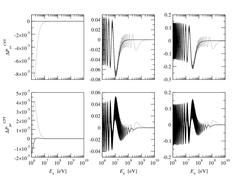
Figure 1: The CPT probability differences $\Delta P_{ee}^{\rm CPT}$ and $\Delta P_{\mu e}^{\rm CPT}$ plotted as functions of the neutrino energy $E_{\nu}$. The baseline lengths used are: 1 km (left column), 250 km (middle column), and 750 km (right column) with $\rho=3\,{\rm g/cm^{3}}$. Dotted curves correspond to numerical calculations using the evolution operator method and Cayley–Hamilton formalism Ohlsson:1999xb ; Ohlsson:1999um ; Ohlsson:2001vp , whereas solid curves correspond to analytical calculations using Eqs. (80) and (83). The fundamental neutrino parameters used are: $\Delta m_{21}^{2}=7.1\cdot 10^{-5}\,{\rm eV}^{2}$, $\Delta m_{31}^{2}=2.5\cdot 10^{-3}\,{\rm eV}^{2}$, $\theta_{12}=34^{\circ}$, $\theta_{13}=9.2^{\circ}$, $\theta_{23}=45^{\circ}$, and $\delta_{\rm CP}=0$.

From these plots we observe that the CPT probability differences increase with increasing baseline length $L$. Furthermore, we note that for increasing neutrino energy $E_{\nu}$ the extrinsic CPT violation effects disappear, since the CPT probability differences go to zero in the limit when $E_{\nu}\to\infty$. We also note that $\Delta P_{ee}^{\rm CPT}$ and $\Delta P_{\mu e}^{\rm CPT}$ are basically of the same order of magnitude. In this figure, the numerical curves consist of a modulation of two oscillations: one slow oscillation with larger amplitude and lower frequency and another fast oscillation with smaller amplitude and higher frequency. On the other hand, the analytical curves consist of one oscillation only and they are therefore not able to reproduce the oscillations with smaller amplitudes and higher frequencies. However, the agreement between the two curves are very good considering the oscillations with larger amplitudes and lower frequencies. In principle, the analytical curves are running averages of the numerical ones, and in fact, the fast oscillations cannot be resolved by any realistic detector due to limited energy resolution making the analytical calculations excellent approximations of the numerical ones.

Let us now investigate some of the most interesting experiments in more detail for which the extrinsic CPT violation effects may be sizeable. In Fig. 2, we plot the CPT probability difference $\Delta P_{ee}^{\rm CPT}$ as functions of both the neutrino energy $E_{\nu}$ and the baseline length $L$ centered around values of these parameters characteristic for the KamLAND experiment.

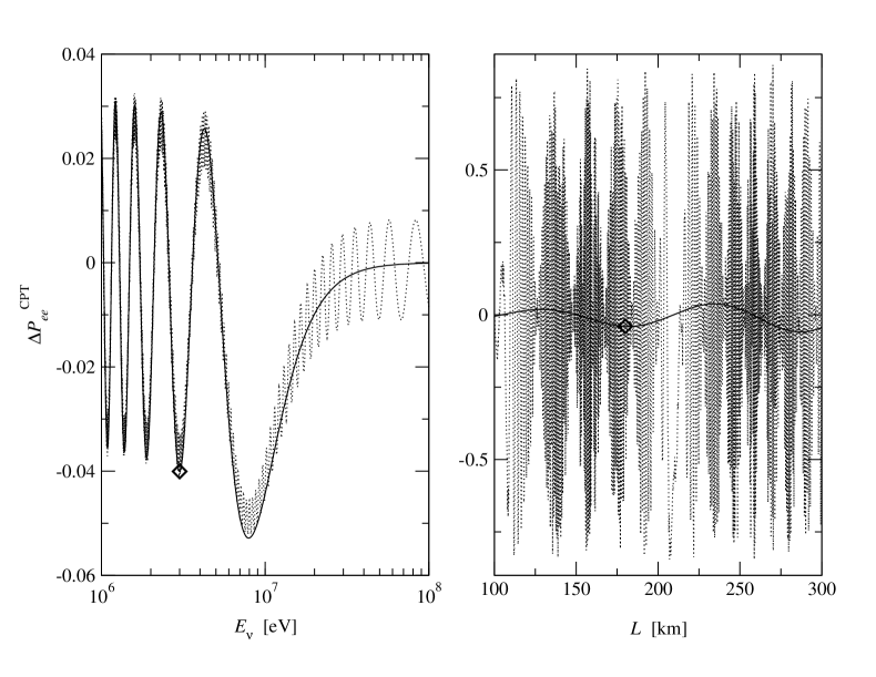
Figure 2: The CPT probability difference $\Delta P_{ee}^{\rm CPT}$ for the KamLAND experiment. The left-hand side plot shows its dependence on the neutrino energy $E_{\nu}$, whereas the right-hand side plot shows its dependence on the baseline length $L$. The solid and dotted curves are analytical and numerical results, respectively. The diamonds (’$\diamond$’) indicate the central values of the KamLAND experiment. The parameters used are the same as for Fig. 1.

We observe that for neutrino energies around the average neutrino energy of the KamLAND experiment the CPT probability difference $\Delta P_{ee}^{\rm CPT}$ could be as large as 3 % - 5 % making the extrinsic CPT violation non-negligible. This means that the transition probabilities $P(\nu_{e}\to\nu_{e})$ and $P(\bar{\nu}_{e}\to\bar{\nu}_{e})$ are not equal to each other for energies and baseline lengths typical for the KamLAND experiment. Thus, if one would be able to find a source of electron neutrinos with the same neutrino energy as the reactor electron antineutrinos coming from the KamLAND experiment, then one would be able to measure such effects. Furthermore, for the KamLAND experiment the agreement between the analytical formula (80) and the low-energy approximation (85) is excellent, i.e., it is not possible to distinguish the results of these formulas from each other in the plots.

Next, in Figs. 3 - 6, we present some plots for the topical accelerator long baseline experiments BNL NWG, JHF-Kamioka, K2K, and NuMI, which have approximately the same neutrino energies, but different baseline lengths. In these figures, we plot the CPT probability difference $\Delta P_{\mu e}^{\rm CPT}$ as functions of the neutrino energy $E_{\nu}$ and the baseline length $L$ as well as the neutrino energy $E_{\nu}$ for three different values of the CP violation phase $\delta_{\rm CP}$ corresponding to no CP violation ($\delta_{\rm CP}=0$), “intermediate” CP violation ($\delta_{\rm CP}=\tfrac{\pi}{4}$), and maximal CP violation ($\delta_{\rm CP}=\tfrac{\pi}{2}$), respectively. We note that in all cases the low-energy approximation curves are upper envelopes to the analytical curves. Furthermore, we note that the CPT probability difference $\Delta P_{\mu e}^{\rm CPT}$ is larger for long baseline experiments with longer baseline lengths and it does not change radically for different values of the CP violation phase $\delta_{\rm CP}$.

Figure 3: The CPT probability difference $\Delta P_{\mu e}^{\rm CPT}$ for the BNL NWG experiment (baseline length: 2540 km). The left-hand side plot shows its dependence on the neutrino energy $E_{\nu}$ (solid curve = analytical calculation, dashed curve = low-energy approximation), the middle plot shows its dependence on the baseline length $L$ (solid curve = analytical calculation, dashed curve = low-energy approximation), and the right-hand side plot shows the dependence on $E_{\nu}$ for three different values of $\delta_{\rm CP}$: $0$ (solid curve), $\tfrac{\pi}{4}$ (dotted curve), and $\tfrac{\pi}{2}$ (dashed curve). The diamonds (’$\diamond$’) indicate the central values of the BNL NWG experiment. The other parameters used are the same as for Fig. 1.

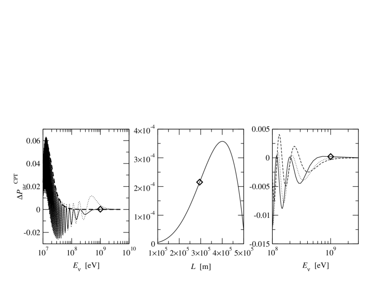
Figure 4: The CPT probability difference $\Delta P_{\mu e}^{\rm CPT}$ for the JHF-Kamioka experiment. The left-hand side plot shows its dependence on the neutrino energy $E_{\nu}$ (dotted curve = numerical calculation, solid curve = analytical calculation, and dashed curve = low-energy approximation), the middle plot shows its dependence on the baseline length $L$ (solid curve = analytical calculation), and the right-hand side plot shows the dependence on $E_{\nu}$ for three different values of $\delta_{\rm CP}$: $0$ (solid curve), $\tfrac{\pi}{4}$ (dotted curve), and $\tfrac{\pi}{2}$ (dashed curve). The diamonds (’$\diamond$’) indicate the central values of the JHF-Kamioka experiment. The other parameters used are the same as for Fig. 1.

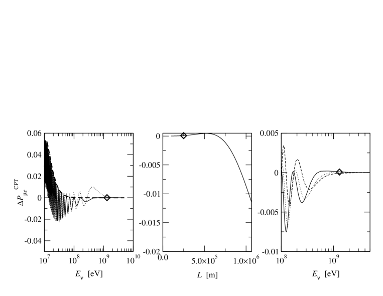
Figure 5: The CPT probability difference $\Delta P_{\mu e}^{\rm CPT}$ for the K2K experiment. The left-hand side plot shows its dependence on the neutrino energy $E_{\nu}$ (dotted curve = numerical calculation, solid curve = analytical calculation, and dashed curve = low-energy approximation), the middle plot shows its dependence on the baseline length $L$ (solid curve = analytical calculation), and the right-hand side plot shows the dependence on $E_{\nu}$ for three different values of $\delta_{\rm CP}$: $0$ (solid curve), $\tfrac{\pi}{4}$ (dotted curve), and $\tfrac{\pi}{2}$ (dashed curve). The diamonds (’$\diamond$’) indicate the central values of the K2K experiment. The other parameters used are the same as for Fig. 1.

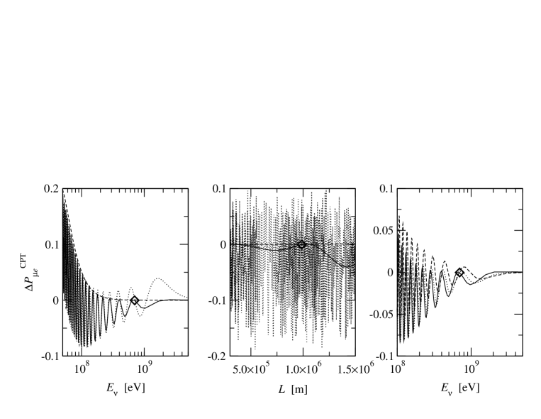
Figure 6: The CPT probability difference $\Delta P_{\mu e}^{\rm CPT}$ for the NuMI Phase II experiment. The left-hand side plot shows its dependence on the neutrino energy $E_{\nu}$ (dotted curve = numerical calculation, solid curve = analytical calculation, and dashed curve = low-energy approximation), the middle plot shows its dependence on the baseline length $L$ (dotted curve = numerical calculation, solid curve = analytical calculation, and dashed curve = low-energy approximation), and the right-hand side plot shows the dependence on $E_{\nu}$ for three different values of $\delta_{\rm CP}$: $0$ (solid curve), $\tfrac{\pi}{4}$ (dotted curve), and $\tfrac{\pi}{2}$ (dashed curve). The diamonds (’$\diamond$’) indicate the central values of the NuMI Phase II experiment. The other parameters used are the same as for Fig. 1.

Finally, in Fig. 7, we present numerical calculations shown as density plots of the CPT probability differences for neutrinos traversing the Earth, which are functions of the nadir angle $h$ and the neutrino energy $E_{\nu}$.

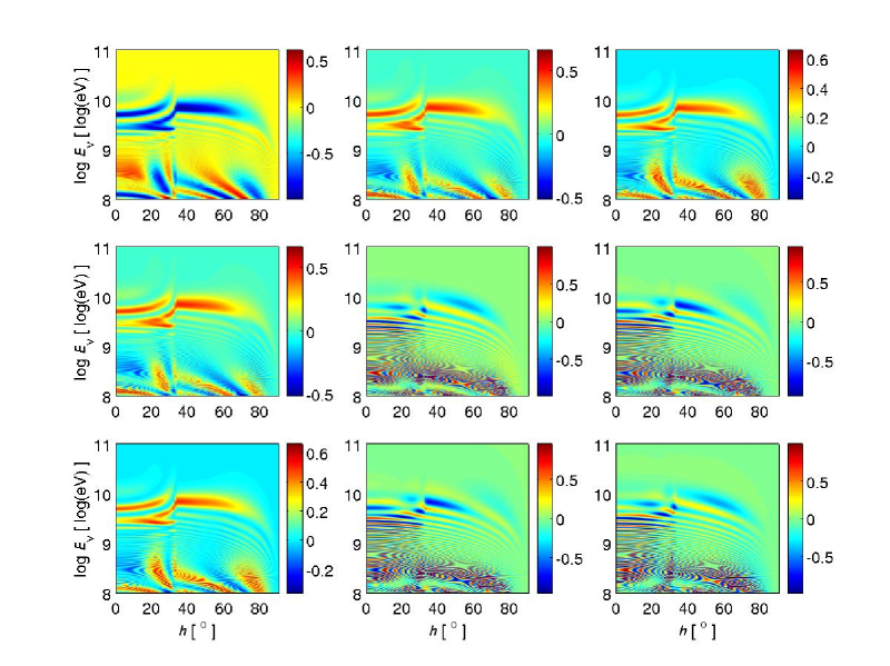
Figure 7: The CPT probability differences $\Delta P_{\alpha\beta}^{\rm CPT}$ ($\alpha,\beta=e,\mu,\tau$) plotted as functions of the nadir angle $h$ and the neutrino energy $E_{\nu}$. The different plots show: $\Delta P_{ee}^{\rm CPT}$ (upper-left), $\Delta P_{e\mu}^{\rm CPT}$ (upper-middle), $\Delta P_{e\tau}^{\rm CPT}$ (upper-right), $\Delta P_{\mu e}^{\rm CPT}$ (middle-left), $\Delta P_{\mu\mu}^{\rm CPT}$ (middle-middle), $\Delta P_{\mu\tau}^{\rm CPT}$ (middle-right), $\Delta P_{\tau e}^{\rm CPT}$ (down-left), $\Delta P_{\mu\tau}^{\rm CPT}$ (down-middle), and $\Delta P_{\tau\tau}^{\rm CPT}$ (down-right). The fundamental neutrino parameters used are: $\Delta m_{21}^{2}=7.1\cdot 10^{-5}\,{\rm eV}^{2}$, $\Delta m_{31}^{2}=2.5\cdot 10^{-3}\,{\rm eV}^{2}$, $\theta_{12}=34^{\circ}$, $\theta_{13}=9.2^{\circ}$, $\theta_{23}=45^{\circ}$, and $\delta_{\rm CP}=0$. Furthermore, we have used the mantle-core-mantle step-function approximation of the Earth matter density profile.

The numerical calculations are based on the evolution operator method and Cayley–Hamilton formalism introduced and developed in Refs. Ohlsson:1999xb ; Ohlsson:1999um ; Ohlsson:2001vp and the parameter values used are given in the figure caption. The nadir angle $h$ is related to the baseline length $L$ as follows. A nadir angle of $h=0$ corresponds to a baseline length of $L=2R_{\oplus}$, whereas $h=90^{\circ}$ corresponds to $L=0$. As $h$ varies from 0 to $90^{\circ}$, the baseline length $L$ becomes shorter and shorter. At an angle larger than $h_{0}\equiv\arcsin\tfrac{r}{R_{\oplus}}\simeq 33.17^{\circ}$, the baseline no longer traverse the core of the Earth. The CPT probability differences in Fig. 7 might be of special interest for atmospheric (and to some extent solar) neutrino oscillation studies, since the plots cover all nadir angle values and neutrino energies between 100 MeV and 100 GeV. We note from these plots that for some specific values of the nadir angle and the neutrino energy the CPT violation effects are rather sizeable.

IV Summary and Conclusions

In conclusion, we have studied extrinsic CPT violation in three flavor neutrino oscillations, i.e., CPT violation induced purely by matter in an intrinsically CPT-conserving context. This has been done by studying the CPT probability differences for arbitrary matter density profiles in general and for constant matter density profiles and to some extent step-function matter density profiles in particular. We have used an analytical approximation based on first order perturbation theory and a low-energy approximation derived from this approximation as well as numerical calculations using the evolution operator method and Cayley–Hamilton formalism. The different methods have then been applied to a number of accelerator and reactor long baseline experiments as well as possible future neutrino factory setups. In addition, their validity and usefulness have been discussed. Furthermore, atmospheric and solar neutrinos have been studied numerically using a step-function matter density profile approximation to the PREM matter density profile. Our results show that the extrinsic CPT probability differences can be as large as 5 % for certain experiments, but be completely negligible for other experiments. Moreover, we have found that in general the CPT probability differences increase with increasing baseline length and decrease with increasing neutrino energy. All this implies that extrinsic CPT violation may affect neutrino oscillation experiments in a significant way. Therefore, we propose to the experimental collaborations to investigate the effects of extrinsic CPT violation in their respective experimental setups. However, it seems that for most neutrino oscillation experiments extrinsic CPT violation effects can safely be ignored.

Finally, we want to mention that in this paper, we have assumed that the CPT invariance theorem holds, which means that there will be no room for intrinsic CPT violation effects in our study, and therefore, the CPT probability differences will only contain extrinsic CPT violation effects due to matter effects. However, it has been suggested in the literature that there might be small intrinsic CPT violation effects in neutrino oscillations Coleman:1998ti ; Barger:2000iv , which might be entangled with the extrinsic CPT violation effects. The question if such intrinsic and the extrinsic CPT violation effects could be disentangled from each other in, for example, realistic long-baseline neutrino oscillation experiments is still open Xing:2001ys and it was not the purpose of the present study. Actually, this deserves an own complete systematic study. However, such a study would be highly model dependent, since intrinsic CPT violation is not present in the SM. Furthermore, it should be noted that in the above mentioned references, Refs. Coleman:1998ti ; Barger:2000iv , the intrinsic CPT violation effects were only studied in neutrino oscillations with two flavors and not with three.

Appendix A Evolution Operators

Neutrino oscillations are governed by the Schrödinger equation [see Eq. (32)]

$${\rm i}\frac{\mathrm{d}}{\mathrm{d}t}|\nu(t)\rangle=\mathscr{H}(t)|\nu(t)\rangle.$$ (113)

Inserting $|\nu(t)\rangle=S(t,t_{0})|\nu(t_{0})\rangle$ [Eq. (34)] yields the Schrödinger equation for the evolution operator

$${\rm i}\frac{\mathrm{d}}{\mathrm{d}t}S(t,t_{0})=\mathscr{H}(t)S(t,t_{0}),$$ (114)

which we write in flavor basis as

$${\rm i}\frac{\mathrm{d}}{\mathrm{d}t}S_{f}(t,t_{0})={\mathscr{H}}_{f}(t)S_{f}(t,t_{0}).$$ (115)

In what follows, we will assume that the number of neutrino flavors is equal to three, i.e., $n=3$. Thus, the total Hamiltonian in flavor basis for neutrinos is given by

$${\mathscr{H}}_{f}(t)=H_{f}+V_{f}(t)=UH_{m}U^{\dagger}+V_{f}(t),$$ (116)

where

$$H_{m}=\left(\begin{matrix}0&0&0\\ 0&\delta&0\\ 0&0&\Delta\end{matrix}\right)\quad\mbox{and}\quad V_{f}(t)=\left(\begin{matrix}V(t)&0&0\\ 0&0&0\\ 0&0&0\end{matrix}\right)$$

are the free Hamiltonian in mass basis and the matter potential in flavor basis, respectively, and $U$ is the leptonic mixing matrix. Here $\delta\equiv\frac{\Delta m_{21}^{2}}{2E_{\nu}}$, $\Delta\equiv\frac{\Delta m_{31}^{2}}{2E_{\nu}}$, and $V(t)=\sqrt{2}G_{F}N_{e}(t)$ is the charged-current contribution of electron neutrinos to the matter potential, where $G_{F}\simeq 1.16639\cdot 10^{-23}\,{\rm eV}^{-2}$ is the Fermi weak coupling constant and $N_{e}(t)=\frac{Y_{e}}{m_{N}}\rho(t)$ is the electron number density with $Y_{e}$ being average number of electrons per nucleon (in the Earth: $Y_{e}\simeq\tfrac{1}{2}$), $m_{N}\simeq 939.565330\,{\rm MeV}$ the nucleon mass, and $\rho\equiv\rho(t)$ the matter density. The sign of the matter potential depends on the presence of neutrinos or antineutrinos. In the case of antineutrinos, one has to change the sign by the replacement $V(t)\to-V(t)$. Thus, the the total Hamiltonian in flavor basis for antineutrinos is given by

$$\bar{\mathscr{H}}_{f}(t)=H_{f}-V_{f}(t)=UH_{m}U^{\dagger}-V_{f}(t).$$ (117)

Decomposing $U=O_{23}U_{13}O_{12}=O_{23}U^{\prime}$, we can write the total Hamiltonian in flavor basis as

$${\mathscr{H}}_{f}(t)=O_{23}\left[U^{\prime}\left(\begin{matrix}0&0&0\\ 0&\delta&0\\ 0&0&\Delta\end{matrix}\right){U^{\prime}}^{\dagger}+\left(\begin{matrix}V(t)&0&0\\ 0&0&0\\ 0&0&0\end{matrix}\right)\right]O_{23}^{T}\equiv O_{23}H(t)O_{23}^{T}.$$ (118)

Here we use the following parameterization for the orthogonal matrices $O_{23}$ and $O_{12}$ and the unitary matrix $U_{13}$

$$O_{23}=\left(\begin{matrix}1&0&0\\ 0&c_{23}&s_{23}\\ 0&-s_{23}&c_{23}\end{matrix}\right),\quad U_{13}=\left(\begin{matrix}c_{13}&0&s_{13}{\rm e}^{-{\rm i}\delta_{\rm CP}}\\ 0&1&0\\ -s_{13}{\rm e}^{{\rm i}\delta_{\rm CP}}&0&c_{13}\end{matrix}\right),\quad O_{12}=\left(\begin{matrix}c_{12}&s_{12}&0\\ -s_{12}&c_{12}&0\\ 0&0&1\end{matrix}\right),$$

where $s_{ab}\equiv\sin\theta_{ab}$ and $c_{ab}\equiv\cos\theta_{ab}$. Here $\theta_{12}$, $\theta_{13}$, and $\theta_{23}$ are the ordinary vacuum mixing angles and $\delta_{\rm CP}$ is the CP violation phase. This means that $U$ is given by the standard parameterization of the leptonic mixing matrix and $U^{\prime}$ is given by

$$U^{\prime}=\left(\begin{matrix}c_{13}c_{12}&c_{13}s_{12}&s_{13}{\rm e}^{-{\rm i}\delta_{\rm CP}}\\ -s_{12}&c_{12}&0\\ -s_{13}c_{12}{\rm e}^{{\rm i}\delta_{\rm CP}}&-s_{13}s_{12}{\rm e}^{{\rm i}\delta_{\rm CP}}&c_{13}\end{matrix}\right).$$ (119)

Inserting ${\mathscr{H}}_{f}(t)=O_{23}H(t)O_{23}^{T}$ into the Schrödinger equation, we obtain

$${\rm i}\frac{\mathrm{d}}{\mathrm{d}t}S(t,t_{0})=H(t)S(t,t_{0}),$$ (120)

where $S(t,t_{0})\equiv O_{23}^{T}S_{f}(t,t_{0})O_{23}$. Thus, the Hamiltonian $H(t)$ can be written as

$$H(t)=\left(\begin{matrix}c_{13}^{2}s_{12}^{2}\delta+s_{13}^{2}\Delta+V(t)&c_{13}c_{12}s_{12}\delta&c_{13}s_{13}\left(\Delta-s_{12}^{2}\delta\right){\rm e}^{-{\rm i}\delta_{\rm CP}}\\ c_{13}c_{12}s_{12}\delta&c_{12}^{2}\delta&-s_{13}c_{12}s_{12}{\rm e}^{-{\rm i}\delta_{\rm CP}}\delta\\ c_{13}s_{13}\left(\Delta-s_{12}^{2}\delta\right){\rm e}^{{\rm i}\delta_{\rm CP}}&-s_{13}c_{12}s_{12}{\rm e}^{{\rm i}\delta_{\rm CP}}\delta&s_{13}^{2}s_{12}^{2}\delta+c_{13}^{2}\Delta\end{matrix}\right).$$ (121)

Series expansions of $s_{13}$ and $c_{13}$ when $\theta_{13}$ is small, i.e., $s_{13}=\theta_{13}+{\mathcal{O}}(\theta_{13}^{3})$ and $c_{13}=1+{\mathcal{O}}(\theta_{13}^{2})$, gives up to second order in $\theta_{13}$

$$H(t)\simeq\left(\begin{matrix}\delta s_{12}^{2}+V(t)&\delta c_{12}s_{12}&\theta_{13}\left(\Delta-\delta s_{12}^{2}\right){\rm e}^{-{\rm i}\delta_{\rm CP}}\\ \delta c_{12}s_{12}&\delta c_{12}^{2}&-\theta_{13}\delta c_{12}s_{12}{\rm e}^{-{\rm i}\delta_{\rm CP}}\\ \theta_{13}\left(\Delta-\delta s_{12}^{2}\right){\rm e}^{{\rm i}\delta_{\rm CP}}&-\theta_{13}\delta c_{12}s_{12}{\rm e}^{{\rm i}\delta_{\rm CP}}&\Delta\end{matrix}\right).$$ (122)

Separating $H(t)$ in independent and dependent parts of $\theta_{13}$ yields

$$H(t)=H_{0}(t)+H^{\prime},\quad H^{\prime}=H_{1}+H_{2},$$ (123)

where

$$H_{0}(t) = \left(\begin{matrix}s_{12}^{2}\delta+V(t)&c_{12}s_{12}\delta&0\\ c_{12}s_{12}\delta&c_{12}^{2}\delta&0\\ 0&0&\Delta\end{matrix}\right)\equiv\left(\begin{matrix}h(t)&\begin{matrix}0\\ 0\end{matrix}\\ \begin{matrix}0&0\end{matrix}&\Delta\end{matrix}\right),$$ (124)

$$H_{1} = \left(\begin{matrix}0&0&\theta_{13}\left(\Delta-s_{12}^{2}\delta\right){\rm e}^{-{\rm i}\delta_{\rm CP}}\\ 0&0&-\theta_{13}c_{12}s_{12}{\rm e}^{-{\rm i}\delta_{\rm CP}}\delta\\ \theta_{13}\left(\Delta-s_{12}^{2}\delta\right){\rm e}^{{\rm i}\delta_{\rm CP}}&-\theta_{13}c_{12}s_{12}{\rm e}^{{\rm i}\delta_{\rm CP}}\delta&0\end{matrix}\right)$$ (125)

$$\equiv \left(\begin{matrix}0&0&a\\ 0&0&b\\ a^{\ast}&b^{\ast}&0\end{matrix}\right),$$

$$H_{2} = {\mathcal{O}}(\theta_{13}^{2}).$$ (126)

Here the Hamiltonian $H_{1}$ is of order $\theta_{13}$, whereas the Hamiltonian $H_{2}$ is of order $\theta_{13}^{2}$. Note that the Hamiltonian $H^{\prime}$ is independent of time $t$. Furthermore, the time-dependent Hamiltonian $H_{0}(t)$ is only dependent on the mixing angle $\theta_{12}$.

Inserting Eq. (123) as well as $S(t,t_{0})\equiv S_{0}(t,t_{0})S_{1}(t,t_{0})$ into Eq. (120) gives

$${\rm i}\left(\frac{\mathrm{d}}{\mathrm{d}t}S_{0}(t,t_{0})\right)S_{1}(t,t_{0})+{\rm i}S_{0}(t,t_{0})\frac{\mathrm{d}}{\mathrm{d}t}S_{1}(t,t_{0})$$ (127)

$$= H_{0}(t)S_{0}(t,t_{0})S_{1}(t,t_{0})+H_{1}S_{0}(t,t_{0})S_{1}(t,t_{0}).$$

Now, assuming that ${\rm i}\frac{\mathrm{d}}{\mathrm{d}t}S_{0}(t,t_{0})=H_{0}(t)S_{0}(t,t_{0})$ holds implies that we have the equation ${\rm i}\frac{\mathrm{d}}{\mathrm{d}t}S_{1}(t,t_{0})=H_{1}(t)S_{1}(t,t_{0})$, where $H_{1}(t)\equiv S_{0}^{-1}(t,t_{0})H_{1}S_{0}(t,t_{0})$, which can be integrated to give the integral equation

$$S_{1}(t,t_{0}) = \mathbbm{1}-{\rm i}\int_{t_{0}}^{t}H_{1}(t^{\prime})S_{1}(t^{\prime},t_{0})\mathrm{d}t^{\prime}$$ (128)

$$= \mathbbm{1}-{\rm i}\int_{t_{0}}^{t}S_{0}^{-1}(t^{\prime},t_{0})H_{1}S_{0}(t^{\prime},t_{0})S_{1}(t^{\prime},t_{0})\mathrm{d}t^{\prime}.$$

Thus, from first order perturbation theory we obtain Arafune:1997hd ; Akhmedov:2001kd

$$S(t,t_{0})\simeq S_{0}(t,t_{0})-{\rm i}S_{0}(t,t_{0})\int_{t_{0}}^{t}S_{0}^{-1}(t^{\prime},t_{0})H_{1}S_{0}(t^{\prime},t_{0})\mathrm{d}t^{\prime}.$$ (129)

Since we assumed before that ${\rm i}\frac{\mathrm{d}}{\mathrm{d}t}S_{0}(t,t_{0})=H_{0}(t)S_{0}(t,t_{0})$ holds, we have now to find $S_{0}(t,t_{0})$. We observe that the $2\times 2$ submatrix in the upper-left corner of $H_{0}(t)$ in Eq. (124), i.e., $h(t)$, is not traceless. Making this submatrix traceless yields

$$\tilde{H}_{0}(t) = H_{0}(t)-\frac{1}{2}{\rm tr\,}h(t)\mathbbm{1}_{3}$$

$$= \left(\begin{matrix}-\frac{1}{2}(c_{12}^{2}-s_{12}^{2})\delta+\frac{1}{2}V(t)&c_{12}s_{12}\delta&0\\ c_{12}s_{12}\delta&\frac{1}{2}(c_{12}^{2}-s_{12}^{2})\delta-\frac{1}{2}V(t)&0\\ 0&0&\Delta-\frac{1}{2}\left[V(t)+\delta\right]\end{matrix}\right).$$

Note that, in general, any term proportional to the identity matrix $\mathbbm{1}_{3}$ can be added to or subtracted from the Hamiltonian $H_{0}(t)$ without affecting the neutrino oscillation probabilities. In particular, a term such that the $2\times 2$ submatrix $h(t)$ in the upper-left corner of $H_{0}(t)$ becomes traceless [see Eq. (LABEL:eq:tildeH0t)]. Furthermore, note that the new Hamiltonian $\tilde{H}_{0}(t)$ will not be traceless and that the $(3,3)$-element of $H_{0}(t)$ will, of course, also be changed by such a transformation.

Instead of solving ${\rm i}\frac{\mathrm{d}}{\mathrm{d}t}S_{0}(t,t_{0})=H_{0}(t)S_{0}(t,t_{0})$, we have now to solve ${\rm i}\frac{\mathrm{d}}{\mathrm{d}t}S_{0}(t,t_{0})=\tilde{H}_{0}(t)S_{0}(t,t_{0})+\frac{1}{2}{\rm tr\,}h(t)S_{0}(t,t_{0})$. The solution to this equation, $S_{0}(t,t_{0})$, has the general form Akhmedov:1998ui ; Akhmedov:1999uz ; Akhmedov:2001kd

$$S_{0}(t,t_{0})=\left(\begin{matrix}\alpha(t,t_{0})&\beta(t,t_{0})&0\\ -\beta^{\ast}(t,t_{0})&\alpha^{\ast}(t,t_{0})&0\\ 0&0&f(t,t_{0})\end{matrix}\right),$$ (131)

where the functions $\alpha(t,t_{0})$ and $\beta(t,t_{0})$ describe the two flavor neutrino evolution in the $(1,2)$-subsector, in which the $2\times 2$ submatrix $h$ of $H_{0}$ acts as the Hamiltonian. In the end of this appendix, we will derive the analytical expressions for the functions $\alpha(t,t_{0})$ and $\beta(t,t_{0})$. The function $f(t,t_{0})$ can, however, immediately be determined to be

$$f(t,t_{0})={\rm e}^{-{\rm i}\int_{t_{0}}^{t}\tilde{\Delta}(t^{\prime})\mathrm{d}t^{\prime}}\equiv{\rm e}^{-{\rm i}\Phi(t,t_{0})},$$ (132)

where $\tilde{\Delta}(t)\equiv\Delta-\frac{1}{2}\left[V(t)+\delta\right]$ and

$$\Phi(t,t_{0}) \equiv \int_{t_{0}}^{t}\tilde{\Delta}(t^{\prime})\mathrm{d}t^{\prime}=\int_{t_{0}}^{t}\left\{\Delta-\frac{1}{2}\left[V(t^{\prime})+\delta\right]\right\}\mathrm{d}t^{\prime}$$

$$= \left(\Delta-\frac{\delta}{2}\right)\left(t-t_{0}\right)-\frac{1}{2}\int_{t_{0}}^{t}V(t^{\prime})\mathrm{d}t^{\prime}.$$

Now, inserting Eqs. (125) and (131) into Eq. (129) yields

$$S(t,t_{0})\simeq\left(\begin{matrix}\alpha(t,t_{0})&\beta(t,t_{0})&-{\rm i}f(t,t_{0})A(t,t_{0})\\ -\beta^{\ast}(t,t_{0})&\alpha^{\ast}(t,t_{0})&-{\rm i}f(t,t_{0})B(t,t_{0})\\ -{\rm i}f(t,t_{0})C(t,t_{0})&-{\rm i}f(t,t_{0})D(t,t_{0})&f(t,t_{0})\end{matrix}\right),$$ (133)

where

$$A(t,t_{0}) = f^{\ast}(t,t_{0})\big{\{}a\left[\alpha(t,t_{0})I_{\alpha^{\ast},t_{0}}(t,t_{0})+\beta(t,t_{0})I_{\beta^{\ast},t_{0}}(t,t_{0})\right]$$ (134)

$$+ b\left[\beta(t,t_{0})I_{\alpha,t_{0}}(t,t_{0})-\alpha(t,t_{0})I_{\beta,t_{0}}(t,t_{0})\right]\big{\}},$$

$$B(t,t_{0}) = f^{\ast}(t,t_{0})\big{\{}a\left[\alpha^{\ast}(t,t_{0})I_{\beta^{\ast},t_{0}}(t,t_{0})-\beta^{\ast}(t,t_{0})I_{\alpha^{\ast},t_{0}}(t,t_{0})\right]$$ (135)

$$+ b\left[\alpha^{\ast}(t,t_{0})I_{\alpha,t_{0}}(t,t_{0})+\beta^{\ast}(t,t_{0})I_{\beta,t_{0}}(t,t_{0})\right]\big{\}},$$

$$C(t,t_{0}) = a^{\ast}I_{\alpha^{\ast},t_{0}}^{\ast}(t,t_{0})-b^{\ast}I_{\beta,t_{0}}^{\ast}(t,t_{0}),$$ (136)

$$D(t,t_{0}) = a^{\ast}I_{\beta^{\ast},t_{0}}^{\ast}(t,t_{0})+b^{\ast}I_{\alpha,t_{0}}^{\ast}(t,t_{0})$$ (137)

with

$$I_{\varphi,t_{0}}(t,t_{0})=\int_{t_{0}}^{t}\varphi(t^{\prime},t_{0})f(t^{\prime},t_{0})\mathrm{d}t^{\prime},\quad\varphi=\alpha,\alpha^{\ast},\beta,\beta^{\ast}.$$ (138)

Equations (134) and (135) can be further simplified using the following

$$S_{0}(t_{1},t) = S_{0}(t_{1},t_{0})S_{0}^{\dagger}(t,t_{0})$$ (139)

$$= \left(\begin{matrix}\alpha(t_{1},t_{0})&\beta(t_{1},t_{0})&0\\ -\beta^{\ast}(t_{1},t_{0})&\alpha^{\ast}(t_{1},t_{0})&0\\ 0&0&f(t_{1},t_{0})\end{matrix}\right)\left(\begin{matrix}\alpha^{\ast}(t,t_{0})&-\beta(t,t_{0})&0\\ \beta^{\ast}(t,t_{0})&\alpha(t,t_{0})&0\\ 0&0&f^{\ast}(t,t_{0})\end{matrix}\right)$$

$$= \left(\begin{matrix}\alpha(t_{1},t)&\beta(t_{1},t)&0\\ -\beta^{\ast}(t_{1},t)&\alpha^{\ast}(t_{1},t)&0\\ 0&0&f(t_{1},t)\end{matrix}\right).$$

Considering Eq. (139), one immediately finds that

$$\alpha(t_{1},t_{0})\alpha^{\ast}(t,t_{0})+\beta(t_{1},t_{0})\beta^{\ast}(t,t_{0}) = \alpha(t_{1},t),$$ (140)

$$-\alpha(t_{1},t_{0})\beta(t,t_{0})+\beta(t_{1},t_{0})\alpha(t,t_{0}) = \beta(t_{1},t),$$ (141)

$$-\beta^{\ast}(t_{1},t_{0})\alpha^{\ast}(t,t_{0})+\alpha^{\ast}(t_{1},t_{0})\beta^{\ast}(t,t_{0}) = -\beta^{\ast}(t_{1},t),$$ (142)

$$\alpha^{\ast}(t_{1},t_{0})\alpha(t,t_{0})+\beta^{\ast}(t_{1},t_{0})\beta(t,t_{0}) = \alpha^{\ast}(t_{1},t),$$ (143)

$$f(t_{1},t_{0})f^{\ast}(t,t_{0}) = f(t_{1},t).$$ (144)

Thus, using Eqs. (140) - (144) as well as the identity $|f(t,t_{0})|^{2}=f(t,t_{0})f^{\ast}(t,t_{0})=1$, one can write Eqs. (134) and (135) as

$$A(t,t_{0}) = aI_{\alpha^{\ast},t}(t,t_{0})-bI_{\beta,t}(t,t_{0}),$$ (145)

$$B(t,t_{0}) = aI_{\beta^{\ast},t}(t,t_{0})+bI_{\alpha,t}(t,t_{0}).$$ (146)

Now, rotating $S(t,t_{0})$ back to the original basis, one finds the evolution operator for neutrinos in the flavor basis

$$S_{f}(t,t_{0}) = O_{23}^{T}S(t,t_{0})O_{23}$$

$$\simeq \left(\begin{matrix}\alpha&c_{23}\beta-{\rm i}s_{23}fA&-s_{23}\beta-{\rm i}c_{23}fA\\ -c_{23}\beta^{\ast}-{\rm i}s_{23}fC&S_{22}&S_{23}\\ s_{23}\beta^{\ast}-{\rm i}c_{23}fC&S_{32}&S_{33}\end{matrix}\right)\equiv(S_{f,ab}),$$

where

$$S_{22} \equiv c_{23}^{2}\alpha^{\ast}+s_{23}^{2}f-{\rm i}s_{23}c_{23}f(B+D),$$ (148)

$$S_{23} \equiv -s_{23}c_{23}\left(\alpha^{\ast}-f\right)-{\rm i}f\left(c_{23}^{2}B-s_{23}^{2}D\right),$$ (149)

$$S_{32} \equiv -s_{23}c_{23}\left(\alpha^{\ast}-f\right)+{\rm i}f\left(s_{23}^{2}B-c_{23}^{2}D\right),$$ (150)

$$S_{33} \equiv s_{23}^{2}\alpha^{\ast}+c_{23}^{2}f+{\rm i}s_{23}c_{23}f\left(B+D\right)$$ (151)

with the notation $\alpha\equiv\alpha(t,t_{0})$, $\beta\equiv\beta(t,t_{0})$, $f\equiv f(t,t_{0})$, $A\equiv A(t,t_{0})$, $B\equiv B(t,t_{0})$, $C\equiv C(t,t_{0})$, and $D\equiv D(t,t_{0})$.

Similarly, replacing the total Hamiltonian for neutrinos (116) with the total Hamiltonian for antineutrinos (117) in the Schrödinger equation (115), the evolution operator for antineutrinos in the flavor basis becomes

$$\bar{S}_{f}(t,t_{0})\simeq\left(\begin{matrix}\bar{\alpha}&c_{23}\bar{\beta}-{\rm i}s_{23}\bar{f}\bar{A}&-s_{23}\bar{\beta}-{\rm i}c_{23}\bar{f}\bar{A}\\ -c_{23}{\bar{\beta}}^{\ast}-{\rm i}s_{23}\bar{f}\bar{C}&\bar{S}_{22}&\bar{S}_{23}\\ s_{23}{\bar{\beta}}^{\ast}-{\rm i}c_{23}\bar{f}\bar{C}&\bar{S}_{32}&\bar{S}_{33}\end{matrix}\right)\equiv(\bar{S}_{f,ab}),$$ (152)

where

$$\bar{S}_{22} \equiv c_{23}^{2}\bar{\alpha}^{\ast}+s_{23}^{2}\bar{f}-{\rm i}s_{23}c_{23}\bar{f}(\bar{B}+\bar{D}),$$ (153)

$$\bar{S}_{23} \equiv -s_{23}c_{23}\left(\bar{\alpha}^{\ast}-\bar{f}\right)-{\rm i}\bar{f}\left(c_{23}^{2}\bar{B}-s_{23}^{2}\bar{D}\right),$$ (154)

$$\bar{S}_{32} \equiv -s_{23}c_{23}\left(\bar{\alpha}^{\ast}-\bar{f}\right)+{\rm i}\bar{f}\left(s_{23}^{2}\bar{B}-c_{23}^{2}\bar{D}\right),$$ (155)

$$\bar{S}_{33} \equiv s_{23}^{2}\bar{\alpha}^{\ast}+c_{23}^{2}\bar{f}+{\rm i}s_{23}c_{23}\bar{f}\left(\bar{B}+\bar{D}\right)$$ (156)

with the same type of notation as in the neutrino case.

We will now derive the general analytical expressions for the functions $\alpha(t,t_{0})$ and $\beta(t,t_{0})$. In order to perform this derivation, we study the evolution operator in the $(1,2)$-subsector, which is a separate problem in the rotated basis, and its solution is independent from the total three flavor neutrino problem. We assume that the evolution operator in the $(1,2)$-subsector, $S_{(1,2)}(t,t_{0})$, satisfies the Schrödinger equation for neutrinos

$${\rm i}\frac{\mathrm{d}}{\mathrm{d}t}S_{(1,2)}(t,t_{0})=h(t)S_{(1,2)}(t,t_{0}),$$ (157)

where $h(t)$ is the Hamiltonian and it is given by

$$h(t) = \left(\begin{matrix}s_{12}^{2}\delta+V(t)&s_{12}c_{12}\delta\\ s_{12}c_{12}\delta&c_{12}^{2}\delta\end{matrix}\right)$$

$$= \left(\begin{matrix}-\tfrac{1}{2}\left(c_{12}^{2}-s_{12}^{2}\right)\delta+\tfrac{1}{2}V(t)&s_{12}c_{12}\delta\\ s_{12}c_{12}\delta&\tfrac{1}{2}\left(c_{12}^{2}-s_{12}^{2}\right)\delta-\tfrac{1}{2}V(t)\end{matrix}\right)+\frac{1}{2}\left[\delta+V(t)\right]\mathbbm{1}_{2},$$

see Eqs. (124) and (LABEL:eq:tildeH0t). Note that the term proportional to the identity matrix $\mathbbm{1}_{2}$ in the Hamiltonian $h(t)$ does not affect neutrino oscillations, since such a term will only generate a phase factor. Thus, we need not consider this term. In addition, note that the same term has been subracted from the Hamiltonian $H_{0}(t)$ [see Eq. (LABEL:eq:tildeH0t)] for the total three flavor neutrino problem. Thus, it also in this case only gives rise to a phase factor in the three flavor neutrino evolution operator $S_{0}(t,t_{0})$ [see Eq. (131)], which does not affect the neutrino oscillations.

The solution to the Schrödinger equation in the $(1,2)$-subsector is

$$S_{(1,2)}(t,t_{0})={\rm e}^{-{\rm i}\int_{t_{0}}^{t}h(t^{\prime})\mathrm{d}t^{\prime}}\equiv{\rm e}^{-{\rm i}H(t,t_{0})},$$ (159)

where the integrated Hamiltonian, $H(t,t_{0})$, is given by

$$H(t,t_{0})=\frac{1}{2}\left(\begin{matrix}-\cos 2\theta_{12}\delta(t-t_{0})+\int_{t_{0}}^{t}V(t^{\prime})\mathrm{d}t^{\prime}&\sin 2\theta_{12}\delta(t-t_{0})\\ \sin 2\theta_{12}\delta(t-t_{0})&\cos 2\theta_{12}\delta(t-t_{0})-\int_{t_{0}}^{t}V(t^{\prime})\mathrm{d}t^{\prime}\end{matrix}\right).$$ (160)

Since $H(t,t_{0})$ is a $2\times 2$ matrix, the solution can be written on the following form Akhmedov:2001kd

$$S_{(1,2)}(t,t_{0}) = \cos\sqrt{-\det H(t,t_{0})}\mathbbm{1}_{2}$$ (161)

$$- {\rm i}\frac{1}{\sqrt{-\det H(t,t_{0})}}\sin\sqrt{-\det H(t,t_{0})}H(t,t_{0}),$$

where the determinant of $H(t,t_{0})$, $\det H(t,t_{0})$, is given by

$$\det H(t,t_{0}) = -\frac{1}{4}\left[\cos 2\theta_{12}\delta(t-t_{0})-\int_{t_{0}}^{t}V(t^{\prime})\mathrm{d}t^{\prime}\right]^{2}-\frac{1}{4}\sin^{2}2\theta_{12}\delta^{2}(t-t_{0})^{2}$$ (162)

$$= -\frac{1}{4}\bigg{[}\delta^{2}(t-t_{0})^{2}-2\cos 2\theta_{12}\delta(t-t_{0})\int_{t_{0}}^{t}V(t^{\prime})\mathrm{d}t^{\prime}$$

$$+ \left(\int_{t_{0}}^{t}V(t^{\prime})\mathrm{d}t^{\prime}\right)^{2}\bigg{]}.$$

Furthermore, the eigenvalues of $H(t,t_{0})$ can be found from the characteristic equation $\det(H(t,t_{0})-\Omega\mathbbm{1}_{2})=0$, which yields $\Omega=\pm\sqrt{-\det H(t,t_{0})}$. Note that in vacuum, i.e., $V(t)=0\;\forall t$, it holds that $\left.\Omega^{2}\right|_{V(t)=0}=\tfrac{1}{4}\delta^{2}(t-t_{0})^{2}\equiv\Omega_{\rm vac}^{2}$. Now, if one writes the evolution operator $S_{(1,2)}(t,t_{0})$ as

$$S_{(1,2)}(t,t_{0})=\left(\begin{matrix}\alpha(t,t_{0})&\beta(t,t_{0})\\ -\beta^{\ast}(t,t_{0})&\alpha^{\ast}(t,t_{0})\end{matrix}\right),$$ (163)

then, using Eq. (161), one can identify the functions $\alpha(t,t_{0})$ and $\beta(t,t_{0})$. We obtain

$$\alpha(t,t_{0}) = \cos\Omega+{\rm i}\frac{\sin\Omega}{2\Omega}\left[\cos 2\theta_{12}\delta(t-t_{0})-\int_{t_{0}}^{t}V(t^{\prime})\mathrm{d}t^{\prime}\right],$$ (164)

$$\beta(t,t_{0}) = -{\rm i}\frac{\sin\Omega}{2\Omega}\sin 2\theta_{12}\delta(t-t_{0}),$$ (165)

where again

$$\Omega = \pm\sqrt{-\det H(t,t_{0})}$$ (166)

$$= \pm\frac{\delta(t-t_{0})}{2}\sqrt{\left[\cos 2\theta_{12}-\frac{1}{\delta(t-t_{0})}\int_{t_{0}}^{t}V(t^{\prime})\mathrm{d}t^{\prime}\right]^{2}+\sin^{2}2\theta_{12}}.$$

Similarly, for antineutrinos the functions $\bar{\alpha}(t,t_{0})$ and $\bar{\beta}(t,t_{0})$ become

$$\bar{\alpha}(t,t_{0}) = \cos\bar{\Omega}+{\rm i}\frac{\sin\bar{\Omega}}{2\bar{\Omega}}\left[\cos 2\theta_{12}\delta(t-t_{0})+\int_{t_{0}}^{t}V(t^{\prime})\mathrm{d}t^{\prime}\right],$$ (167)

$$\bar{\beta}(t,t_{0}) = -{\rm i}\frac{\sin\bar{\Omega}}{2\bar{\Omega}}\sin 2\theta_{12}\delta(t-t_{0}),$$ (168)

which we, in principle, obtain by making the replacement $V(t)\to-V(t)$ in the expressions for the functions $\alpha(t,t_{0})$ and $\beta(t,t_{0})$. Here

$$\bar{\Omega}=\pm\frac{\delta(t-t_{0})}{2}\sqrt{\left[\cos 2\theta_{12}+\frac{1}{\delta(t-t_{0})}\int_{t_{0}}^{t}V(t^{\prime})\mathrm{d}t^{\prime}\right]^{2}+\sin^{2}2\theta_{12}}.$$ (169)

Note that $\Omega$ in Eq. (166) and $\bar{\Omega}$ in Eq. (169) only differ with respect to the sign in front of the integral of the matter potential. Thus, from the expressions for $\Omega$ and $\bar{\Omega}$ we find that

$$\bar{\Omega}^{2}=\Omega^{2}+\cos 2\theta_{12}\delta(t-t_{0})\int_{t_{0}}^{t}V(t^{\prime})\mathrm{d}t^{\prime}.$$ (170)

Let us now consider some special cases when the relation between $\Omega$ and $\bar{\Omega}$ becomes simpler. In the case that

• $t-t_{0}=0$, one finds $\Omega=\bar{\Omega}=0$, which is a trivial and non-interesting case.

• $\delta=0$, we have degenerated neutrino masses $m_{1}=m_{2}$ (and negligible solar mass squared difference) or extremely high neutrino energy and this leads to $\Omega^{2}=\bar{\Omega}^{2}=\frac{1}{4}\left[\int_{t_{0}}^{t}V(t^{\prime})\mathrm{d}t^{\prime}\right]^{2}$, which implies that $\bar{\Omega}=\pm\Omega$. Thus, in addition, we have $\alpha=\cos\Omega-{\rm i}\frac{\sin\Omega}{2\Omega}\int_{t_{0}}^{t}V(t^{\prime})\mathrm{d}t^{\prime}$, $\bar{\alpha}=\cos\Omega+{\rm i}\frac{\sin\Omega}{2\Omega}\int_{t_{0}}^{t}V(t^{\prime})\mathrm{d}t^{\prime}=\alpha^{\ast}$, and $\beta=\bar{\beta}=0$.

• $\cos 2\theta_{12}=0$ (e.g., $\theta_{12}=45^{\circ}$), we have maximal mixing in the $(1,2)$-subsector and this leads to $\Omega^{2}=\bar{\Omega}^{2}=\frac{1}{4}\delta^{2}(t-t_{0})^{2}+\frac{1}{4}\left[\int_{t_{0}}^{t}V(t^{\prime})\mathrm{d}t^{\prime}\right]^{2}$, which again implies that $\bar{\Omega}=\pm\Omega$. In this case, we find $\alpha=\cos\Omega-{\rm i}\frac{\sin\Omega}{2\Omega}\int_{t_{0}}^{t}V(t^{\prime})\mathrm{d}t^{\prime}$, $\bar{\alpha}=\cos\Omega+{\rm i}\frac{\sin\Omega}{2\Omega}\int_{t_{0}}^{t}V(t^{\prime})\mathrm{d}t^{\prime}=\alpha^{\ast}$, and $\beta=\bar{\beta}=-{\rm i}\frac{\sin\Omega}{2\Omega}\delta(t-t_{0})$.

• $\int_{t_{0}}^{t}V(t^{\prime})\mathrm{d}t^{\prime}=0$, one obtains $\Omega^{2}=\bar{\Omega}^{2}=\frac{1}{4}\delta^{2}(t-t_{0})^{2}$, which also implies that $\bar{\Omega}=\pm\Omega$. Furthermore, one has $\alpha=\bar{\alpha}=\cos\Omega+{\rm i}\frac{\sin\Omega}{2\Omega}\cos 2\theta_{12}\delta(t-t_{0})$ and $\beta=\bar{\beta}=-{\rm i}\frac{\sin\Omega}{2\Omega}\sin 2\theta_{12}\delta(t-t_{0})$.

In addition, if we have close to maximal mixing, i.e., $\theta_{12}\lesssim 45^{\circ}$, then we can write $\theta_{12}=\frac{\pi}{4}-\epsilon$, where $\epsilon$ is a small parameter. Making a series expansion with the parameter $\epsilon$ as a small expansion parameter, we obtain

$$\cos 2\theta_{12} = 2\epsilon-\frac{4}{3}\epsilon^{3}+\mathcal{O}(\epsilon^{5}),$$ (171)

$$\bar{\Omega} = \pm\left[\Omega+\frac{1}{\Omega}\delta(t-t_{0})\int_{t_{0}}^{t}V(t^{\prime})\mathrm{d}t^{\prime}\epsilon+\mathcal{O}(\epsilon^{2})\right].$$ (172)

References

- (1) S. R. Coleman and S. L. Glashow, Phys. Lett. B405, 249 (1997), hep-ph/9703240.
- (2) S. R. Coleman and S. L. Glashow, Phys. Rev. D59, 116008 (1999), hep-ph/9812418.
- (3) V. D. Barger, S. Pakvasa, T. J. Weiler, and K. Whisnant, Phys. Rev. Lett. 85, 5055 (2000), hep-ph/0005197.
- (4) H. Murayama and T. Yanagida, Phys. Lett. B520, 263 (2001), hep-ph/0010178.
- (5) M. C. Bañuls, G. Barenboim, and J. Bernabéu, Phys. Lett. B513, 391 (2001), hep-ph/0102184.
- (6) G. Barenboim, L. Borissov, J. Lykken, and A. Y. Smirnov, J. High Energy Phys. 10, 001 (2002), hep-ph/0108199.
- (7) G. Barenboim, L. Borissov, and J. Lykken, Phys. Lett. B534, 106 (2002), hep-ph/0201080.
- (8) G. Barenboim, J. F. Beacom, L. Borissov, and B. Kayser, Phys. Lett. B537, 227 (2002), hep-ph/0203261.
- (9) G. Barenboim and J. Lykken, Phys. Lett. B554, 73 (2003), hep-ph/0210411.
- (10) G. Barenboim, L. Borissov, and J. Lykken, hep-ph/0212116.
- (11) S. Pakvasa, hep-ph/0110175.
- (12) Z.-z. Xing, J. Phys. G28, B7 (2002), hep-ph/0112120.
- (13) S. Skadhauge, Nucl. Phys. B639, 281 (2002), hep-ph/0112189.
- (14) S. M. Bilenky et al., Phys. Rev. D65, 073024 (2002), hep-ph/0112226.
- (15) T. Ohlsson, hep-ph/0209150.
- (16) J. N. Bahcall, V. Barger, and D. Marfatia, Phys. Lett. B534, 120 (2002), hep-ph/0201211.
- (17) A. Strumia, Phys. Lett. B539, 91 (2002), hep-ph/0201134.
- (18) I. Mocioiu and M. Pospelov, Phys. Lett. B534, 114 (2002), hep-ph/0202160.
- (19) A. De Gouvêa, Phys. Rev. D66, 076005 (2002), hep-ph/0204077.
- (20) LSND Collaboration, C. Athanassopoulos et al., Phys. Rev. Lett. 77, 3082 (1996), nucl-ex/9605003.
- (21) LSND Collaboration, C. Athanassopoulos et al., Phys. Rev. Lett. 81, 1774 (1998), nucl-ex/9709006.
- (22) LSND Collaboration, A. Aguilar et al., Phys. Rev. D64, 112007 (2001), hep-ex/0104049.
- (23) Super-Kamiokande Collaboration, Y. Fukuda et al., Phys. Rev. Lett. 81, 1562 (1998), hep-ex/9807003.
- (24) Super-Kamiokande Collaboration, Y. Fukuda et al., Phys. Rev. Lett. 82, 2644 (1999), hep-ex/9812014.
- (25) Super-Kamiokande Collaboration, S. Fukuda et al., Phys. Rev. Lett. 85, 3999 (2000), hep-ex/0009001.
- (26) M. Shiozawa, talk given at the XXth International Conference on Neutrino Physics & Astrophysics (Neutrino 2002), Munich, Germany, 2002.
- (27) Super-Kamiokande Collaboration, S. Fukuda et al., Phys. Rev. Lett. 86, 5651 (2001), hep-ex/0103032.
- (28) Super-Kamiokande Collaboration, S. Fukuda et al., Phys. Rev. Lett. 86, 5656 (2001), hep-ex/0103033.
- (29) Super-Kamiokande Collaboration, M. B. Smy, hep-ex/0106064.
- (30) Super-Kamiokande Collaboration, S. Fukuda et al., Phys. Lett. B539, 179 (2002), hep-ex/0205075.
- (31) M. Smy, talk given at the XXth International Conference on Neutrino Physics & Astrophysics (Neutrino 2002), Munich, Germany, 2002.
- (32) SNO Collaboration, Q. R. Ahmad et al., Phys. Rev. Lett. 87, 071301 (2001), nucl-ex/0106015.
- (33) SNO Collaboration, Q. R. Ahmad et al., Phys. Rev. Lett. 89, 011301 (2002), nucl-ex/0204008.
- (34) SNO Collaboration, Q. R. Ahmad et al., Phys. Rev. Lett. 89, 011302 (2002), nucl-ex/0204009.
- (35) A. Hallin, talk given at the XXth International Conference on Neutrino Physics & Astrophysics (Neutrino 2002), Munich, Germany, 2002.
- (36) MiniBooNE Collaboration, http://www-boone.fnal.gov/
- (37) J. N. Bahcall, M. C. Gonzalez-Garcia, and C. Peña-Garay, J. High Energy Phys. 07, 054 (2002), hep-ph/0204314.
- (38) G. Lüders, K. Dan. Vidensk. Selsk. Mat. Fys. Medd. 28, 5 (1954).
- (39) W. Pauli, in Niels Bohr and the Development of Physics, edited by W. Pauli, L. Rosenfeld, and V. Weisskopf (Pergamon, London, 1955).
- (40) J. S. Bell, Proc. R. Soc. London A231, 479 (1955).
- (41) KamLAND Collaboration, K. Eguchi et al., Phys. Rev. Lett. 90, 021802 (2003), hep-ex/0212021.
- (42) J. N. Bahcall, M. C. Gonzalez-Garcia, and C. Peña-Garay, J. High Energy Phys. 02, 009 (2003), hep-ph/0212147.
- (43) E. K. Akhmedov, P. Huber, M. Lindner, and T. Ohlsson, Nucl. Phys. B608, 394 (2001), hep-ph/0105029.
- (44) J. Bernabéu, hep-ph/9904474.
- (45) J. Bernabéu, S. Palomares-Ruiz, A. Perez, and S. T. Petcov, Phys. Lett. B531, 90 (2002), hep-ph/0110071.
- (46) J. Bernabéu and S. Palomares-Ruiz, hep-ph/0112002.
- (47) J. Bernabéu and S. Palomares-Ruiz, Nucl. Phys. Proc. Suppl. 110, 339 (2002), hep-ph/0201090.
- (48) J. Arafune, M. Koike, and J. Sato, Phys. Rev. D56, 3093 (1997), hep-ph/9703351.
- (49) H. Minakata and H. Nunokawa, Phys. Rev. D57, 4403 (1998), hep-ph/9705208.
- (50) H. Minakata and H. Nunokawa, Phys. Lett. B413, 369 (1997), hep-ph/9706281.
- (51) K. R. Schubert, hep-ph/9902215.
- (52) K. Dick, M. Freund, M. Lindner, and A. Romanino, Nucl. Phys. B562, 29 (1999), hep-ph/9903308.
- (53) A. Donini, M. B. Gavela, P. Hernandez, and S. Rigolin, Nucl. Phys. B574, 23 (2000), hep-ph/9909254.
- (54) A. Cervera et al., Nucl. Phys. B579, 17 (2000), hep-ph/0002108; B593, 731(E) (2001).
- (55) H. Minakata and H. Nunokawa, Phys. Lett. B495, 369 (2000), hep-ph/0004114.
- (56) V. D. Barger, S. Geer, R. Raja, and K. Whisnant, Phys. Rev. D63, 033002 (2001), hep-ph/0007181.
- (57) P. M. Fishbane and P. Kaus, Phys. Lett. B506, 275 (2001), hep-ph/0012088.
- (58) M. C. Gonzalez-Garcia, Y. Grossman, A. Gusso, and Y. Nir, Phys. Rev. D64, 096006 (2001), hep-ph/0105159.
- (59) H. Minakata and H. Nunokawa, J. High Energy Phys. 10, 001 (2001), hep-ph/0108085.
- (60) H. Minakata, H. Nunokawa, and S. Parke, Phys. Lett. B537, 249 (2002), hep-ph/0204171.
- (61) K. Kimura, A. Takamura, and H. Yokomakura, Phys. Rev. D66, 073005 (2002), hep-ph/0205295.
- (62) H. Yokomakura, K. Kimura, and A. Takamura, Phys. Lett. B544, 286 (2002), hep-ph/0207174.
- (63) T. Ota and J. Sato, Phys. Rev. D67, 053003 (2003), hep-ph/0211095.
- (64) T. K. Kuo and J. Pantaleone, Phys. Lett. B198, 406 (1987).
- (65) P. I. Krastev and S. T. Petcov, Phys. Lett. B205, 84 (1988).
- (66) S. Toshev, Phys. Lett. B226, 335 (1989).
- (67) S. Toshev, Mod. Phys. Lett. A6, 455 (1991).
- (68) J. Arafune and J. Sato, Phys. Rev. D55, 1653 (1997), hep-ph/9607437.
- (69) M. Koike and J. Sato, hep-ph/9707203.
- (70) S. M. Bilenky, C. Giunti, and W. Grimus, Phys. Rev. D58, 033001 (1998), hep-ph/9712537.
- (71) V. D. Barger, Y.-B. Dai, K. Whisnant, and B.-L. Young, Phys. Rev. D59, 113010 (1999), hep-ph/9901388.
- (72) M. Koike and J. Sato, Phys. Rev. D61, 073012 (2000), hep-ph/9909469.
- (73) O. Yasuda, Acta Phys. Polon. B30, 3089 (1999), hep-ph/9910428.
- (74) J. Sato, Nucl. Instrum. Meth. A451, 36 (2000), hep-ph/9910442.
- (75) M. Koike and J. Sato, Phys. Rev. D62, 073006 (2000), hep-ph/9911258.
- (76) P. F. Harrison and W. G. Scott, Phys. Lett. B476, 349 (2000), hep-ph/9912435.
- (77) V. A. Naumov, Sov. Phys. JETP 74, 1 (1992), zh. Eksp. Teor. Fiz. 101 (1992) 3.
- (78) V. A. Naumov, Int. J. Mod. Phys. D1, 379 (1992).
- (79) H. Yokomakura, K. Kimura, and A. Takamura, Phys. Lett. B496, 175 (2000), hep-ph/0009141.
- (80) S. J. Parke and T. J. Weiler, Phys. Lett. B501, 106 (2001), hep-ph/0011247.
- (81) M. Koike, T. Ota, and J. Sato, Phys. Rev. D65, 053015 (2002), hep-ph/0011387.
- (82) T. Miura, E. Takasugi, Y. Kuno, and M. Yoshimura, Phys. Rev. D64, 013002 (2001), hep-ph/0102111.
- (83) T. Miura, T. Shindou, E. Takasugi, and M. Yoshimura, Phys. Rev. D64, 073017 (2001), hep-ph/0106086.
- (84) A. Rubbia, hep-ph/0106088.
- (85) Z.-z. Xing, Phys. Rev. D64, 093013 (2001), hep-ph/0107005.
- (86) T. Ota, J. Sato, and Y. Kuno, Phys. Lett. B520, 289 (2001), hep-ph/0107007.
- (87) T. Ohlsson, hep-ph/0108048.
- (88) A. Bueno, M. Campanelli, S. Navas-Concha, and A. Rubbia, Nucl. Phys. B631, 239 (2002), hep-ph/0112297.
- (89) J. Sato, eConf C010630, E105 (2001).
- (90) E. K. Akhmedov, hep-ph/0207342.
- (91) H. Minakata, H. Nunokawa, and S. Parke, Phys. Rev. D66, 093012 (2002), hep-ph/0208163.
- (92) P. Huber, J. Phys. G29, 1853 (2003), hep-ph/0210140.
- (93) C. N. Leung and Y. Y. Y. Wong, Phys. Rev. D67, 056005 (2003), hep-ph/0301211.
- (94) S. M. Bilenky and B. Pontecorvo, Phys. Rept. 41, 225 (1978).
- (95) S. M. Bilenky and S. T. Petcov, Rev. Mod. Phys. 59, 671 (1987), 61 (1989) 169(E).
- (96) M. Lindner, hep-ph/0209083 and hep-ph/0210377, and references therein.
- (97) H. Minakata, private communication.
- (98) C. Jarlskog, Phys. Rev. Lett. 55, 1039 (1985).
- (99) C. Jarlskog, Z. Phys. C29, 491 (1985).
- (100) J. N. Bahcall, M. C. Gonzalez-Garcia, and C. Peña-Garay, J. High Energy Phys. 08, 014 (2001), hep-ph/0106258.
- (101) J. N. Bahcall, M. C. Gonzalez-Garcia, and C. Peña-Garay, J. High Energy Phys. 04, 007 (2002), hep-ph/0111150.
- (102) CHOOZ Collaboration, M. Apollonio et al., Phys. Lett. B420, 397 (1998), hep-ex/9711002.
- (103) CHOOZ Collaboration, M. Apollonio et al., Phys. Lett. B466, 415 (1999), hep-ex/9907037.
- (104) CHOOZ Collaboration, M. Apollonio et al., Eur. Phys. J. C27, 331 (2003), hep-ex/0301017.
- (105) A. M. Dziewonski and D. L. Anderson, Phys. Earth Planet. Interiors 25, 297 (1981).
- (106) M. Freund and T. Ohlsson, Mod. Phys. Lett. A15, 867 (2000), hep-ph/9909501, and references therein.
- (107) BNL Neutrino Working Group Collaboration, D. Beavis et al., hep-ex/0205040.
- (108) W. J. Marciano, hep-ph/0108181.
- (109) M. V. Diwan et al., Phys. Rev. D68, 012002 (2003), hep-ph/0303081.
- (110) BooNE Collaboration, E. D. Zimmerman, eConf C0209101, TH05 (2002), hep-ex/0211039.
- (111) BooNE Collaboration, A. O. Bazarko, hep-ex/0210020.
- (112) ICARUS Collaboration, A. Rubbia et al., cERN-SPSLC-96-58.
- (113) ICARUS Collaboration, F. Arneodo et al., hep-ex/0103008.
- (114) OPERA and ICARUS Collaboration, D. Duchesneau, eConf C0209101, TH09 (2002), hep-ex/0209082.
- (115) JHF-Kamioka Collaboration, Y. Itow et al., hep-ex/0106019.
- (116) K2K Collaboration, S. H. Ahn et al., Phys. Lett. B511, 178 (2001), hep-ex/0103001.
- (117) K2K Collaboration, M. H. Ahn et al., Phys. Rev. Lett. 90, 041801 (2003), hep-ex/0212007.
- (118) MINOS Collaboration, S. G. Wojcicki, Nucl. Phys. Proc. Suppl. 91, 216 (2001).
- (119) MINOS Collaboration, V. Paolone, Nucl. Phys. Proc. Suppl. 100, 197 (2001).
- (120) MINOS Collaboration, M. V. Diwan, eConf C0209101, TH08 (2002), hep-ex/0211026.
- (121) NuMI Collaboration, D. Ayres et al., hep-ex/0210005.
- (122) NuTeV Collaboration, S. Avvakumov et al., Phys. Rev. Lett. 89, 011804 (2002), hep-ex/0203018.
- (123) OPERA Collaboration, H. Pessard, Phys. Scripta T93, 59 (2001).
- (124) Palo Verde Collaboration, F. Boehm et al., Prog. Part. Nucl. Phys. 40, 253 (1998).
- (125) Palo Verde Collaboration, F. Boehm et al., Phys. Rev. Lett. 84, 3764 (2000), hep-ex/9912050.
- (126) Palo Verde Collaboration, F. Boehm et al., Phys. Rev. D62, 072002 (2000), hep-ex/0003022.
- (127) Palo Verde Collaboration, F. Boehm et al., Phys. Rev. D64, 112001 (2001), hep-ex/0107009.
- (128) T. Ohlsson and H. Snellman, J. Math. Phys. 41, 2768 (2000), hep-ph/9910546; D42, 2345(E) (2001).
- (129) T. Ohlsson and H. Snellman, Phys. Lett. B474, 153 (2000), hep-ph/9912295; B480, 419(E) (2000).
- (130) T. Ohlsson, Phys. Scripta T93, 18 (2001).
- (131) E. K. Akhmedov, Nucl. Phys. B538, 25 (1999), hep-ph/9805272.
- (132) E. K. Akhmedov, hep-ph/0001264.
- (133) Particle Data Group, K. Hagiwara et al., Phys. Rev. D66, 010001 (2002), http://pdg.lbl.gov/.