The Higgs mass as a function
of the compactification scale

Riccardo Barbieri, Guido Marandella and Michele Papucci

Scuola Normale Superiore and INFN, Piazza dei Cavalieri 7, I-56126 Pisa, Italy

1 Introduction

In the Standard Model (SM) the sensitivity of the Fermi scale $G_{F}^{-1/2}$ to the cut-off $\Lambda$ strongly suggests the presence of new physics close to $G_{F}^{-1/2}$ itself. Since long time the possibility is contemplated that such new physics be represented by supersymmetric particles with masses of order $G_{F}^{-1/2}$. Relatively more recently, the scale of a compactified extra dimension (one or more) has also been put forward to play the same role [1]. In this paper we study, as precisely as possible, the consequences for ElectroWeak Symmetry Breaking (EWSB) from the merging of these two ideas in a definite scheme, as defined in [2] .

This contamination has a main motivation: it allows to describe supersymmetry breaking in terms of a single parameter, $L$, the length of the segment to which the extra-dimension is compactified. Although $L\rightarrow\infty$ is the limit where supersymmetry is recovered, the compactification scale is not the scale above which a supersymmetric spectrum approximately appears, due to the presence of the Kaluza-Klein (KK) modes. There is no such scale. In fact, the KK modes play a crucial role in rendering more precise the supersymmetric softening of the ultraviolet divergences. The introduction of the usual soft supersymmetry-breaking parameters is avoided. Nor there is any need of introducing a supersymmetric $\mu$-parameter, since only one Higgs field gets a non-vanishing vacuum expectation value consistently with all phenomenological requirements and with the supersymmetry constraints [5].

For a theory that is designed to render the Fermi scale insensitive to the cut-off, the connection between $G_{F}^{-1/2}$ and the scale of new physics should be determined as neatly as possible. This is highly desirable not only theoretically but also from a phenomenological and pragmatic point of view, since the possibility to test the theory at the Tevatron or at the LHC crucially depends on this property. This motivates a careful study of the Higgs potential. A peculiar feature that emerges from this study is the gap that can result between $1/L$ and $G_{F}^{-1/2}$ or, even more so, the Higgs mass. Although anticipated in [2], the precise assessment of this property as the equally precise determination of the Higgs mass as a function of $1/L$ – our main goals in this paper – require the two loop calculation of the Higgs potential described below.

The paper is organized as follows. The model is defined in Sect. 2. In Sect. 3 the Higgs potential is calculated to two loops accuracy in $\alpha_{s}=g_{s}^{2}/(4\pi)$ and $\alpha_{t}=y_{t}^{2}/(4\pi)$ with the top supermultiplet exactly localized at $y=0$. In Sect. 4 a quasi localized top is introduced and both the Higgs mass and the determination of the Fermi scale are studied as function of $1/L=2\div 4$ TeV. The issue of the uncertainties is explicitly addressed in Sect. 4.3. In Sect. 5 the possibility is considered of a lower value of the compactification scale, allowing for the presence of a common mass for the Higgs hypermultiplets. The spectrum of the model is given in Sect. 6. The summary and the conclusions are drawn in Sect 7.

2 The Model

We consider a 5D, $SU(3)\times SU(2)\times U(1)$ invariant theory with every multiplet of the SM, gauge, matter or Higgs, promoted to a $N=1$ supermultiplet (hypermultiplet). The fifth dimension is meant to be compactified on a segment parameterized by $y\in\left[0,L\right]$ .

As advocated long ago by Scherk and Schwarz [6], we break supersymmetry by boundary conditions at $y=0,L$ that distinguish the different fields in every hypermultiplet. Given the 5D gauge theory, there is a single choice of these boundary conditions, consistent with the symmetries of the theory and with supergravity, that leads to a massless spectrum identical to the SM one [5]. This non trivial property is at variance with what happens when global supersymmetry is spontaneously broken in a 4D theory, where a hidden sector and a mediation mechanism of supersymmetry breaking have to be introduced. With these boundary conditions, summarized in Table 1, every field acquires, in the effective 4D picture, a definite KK tower. The first KK states of the SM particles are at $\pi/L$, whereas the extra particles implied by supersymmetry and/or Poincaré invariance are at $\pi/(2L)$ or higher.

$\psi_{M}$, $\phi_{H}$, $A^{\mu}$	$\phi_{M}$, $\psi_{H}$, $\lambda$	$\phi^{c}_{M}$, $\psi^{c}_{H}$, $\lambda^{c}$	$\psi^{c}_{M}$, $\phi^{c}_{H}$, $\phi_{\Sigma}$
$(+,+)$	$(+,-)$	$(-,+)$	$(-,-)$

Table 1: Boundary conditions for gauge $(A_{\mu},\lambda,\lambda^{c},\phi_{\Sigma})$, matter $(\psi_{M},\phi_{M},\psi_{M}^{c},\phi_{M}^{c})$ and Higgs $(\phi_{H},\psi_{H},\phi_{H}^{c},\psi_{H}^{c})$ multiplets at $y=0$ and $y=L$.

A theory thus defined has a divergent Fayet-Iliopoulos term induced at one loop [7], which can be canceled by introducing a second Higgs-like hypermultiplet, $H_{c}$. In this case one obtains, at tree level, two (massless) Higgs-like scalars as in the Minimal Supersymmetric Standard Model (MSSM). At variance with the MSSM, however, the second Higgs-like scalar does not get a vacuum expectation value (VEV) and plays no role in EWSB.

Without affecting the massless spectrum, it is consistent to introduce suitable supersymmetric mass terms $M$ for the matter hypermultiplets [8]. They deform the massive spectrum as well as the wave function in $y$ of every state [4]. The wave function of the massless states (the matter fermions) becomes an exponential, $\psi_{0}(y)\propto\left|M\right|^{1/2}e^{-My+(M-\left|M\right|)L/2}$, so that in the large $ML$ limit, $|ML|\gg 1$, the massless fermion gets localized on one of the two boundaries, $y=0$ or $y=L$, depending on the sign of $M$. At the same time a chiral $N=1$, $4D$ supermultiplet is recovered with one scalar becoming also massless and localized. All the other states get a heavy mass, increasing like $M$. These hypermultiplet masses, in general different for every matter multiplet, are non renormalized parameters and could be fixed in a more fundamental theory. Not to introduce again a Fayet-Iliopoulos term they have to satisfy simple conditions [8]: e.g. a common mass for the quark hypermultiplets of a given generation, $M_{Q_{i}}$, for the lepton hypermultiplets, $M_{L_{i}}$, and for the Higgs-like hypermultiplets $M_{H}$. We stick to this configuration in the following.

The top Yukawa coupling, necessarily localized at one of the two boundaries, say $y=0$, is the source of EWSB, which is therefore influenced by the mass terms of the top quark hypermultiplets $Q$ and $U$, $M_{Q_{3}}\equiv M$. We shall take them quite closely localized at $y=0$, with $ML\gtrsim 1$ for most of the paper. For this reason, it is a significant approximation to consider first what happens when $Q$ and $U$ are exactly localized.

3 The Higgs potential with a top localized on one boundary

Symbolically, the reference Lagrangian is

$$\mathcal{L}=\mathcal{L}_{5D}^{N=1}\left(\textrm{gauge}\oplus\textrm{Higgs}\right)+\mathcal{L}_{4D}^{N=1}\left(Q\oplus U\right)\delta(y)$$ (1)

where the $4D$, $N=1$ supersymmetric Lagrangian for the $Q,U$ chiral supermultiplets includes the top Yukawa coupling

$$\mathcal{L}_{4D}^{N=1}\left(Q\oplus U\right)=\int\textrm{d}^{4}\theta Q^{\dagger}e^{V}Q+\int\textrm{d}^{4}\theta U^{\dagger}e^{V}U+\left[\int\textrm{d}^{2}\theta\lambda_{t}HQU+\textrm{h.c.}\right]$$ (2)

We ignore for the time being possible kinetic terms for the gauge and Higgs multiplets also localized at the boundaries (See Sect. 4.3).

With the boundary conditions in Table 1, after the integration over $y$, the tree level potential for the real part of the zero mode of the Higgs field is

$$V^{\textrm{tree}}(h^{2})=\frac{g^{2}+g^{\prime 2}}{32}h^{4}$$ (3)

We are interested in the effective potential $V(h^{2})$ which, expanded around $h=v$, gives

$$V(h^{2})\simeq 2v\;V^{\prime}(v^{2})\;h+\left[V^{\prime}(v^{2})+2v^{2}\;V^{\prime\prime}(v^{2})\right]\;h^{2}$$ (4)

Hence

$$V^{\prime}(v^{2})=0$$ (5)

is the equation which determines $v$ or the Fermi scale $G_{F}^{-1/2}$ and

$$m_{h}^{2}=4v^{2}\;V^{\prime\prime}(v^{2})$$ (6)

is the physical Higgs squared mass. We aim to an accuracy of a few percent in $V^{\prime}$ and $V^{\prime\prime}$.

The 1 loop electroweak contribution to $V^{\prime}$ has been computed in [9]

$$\delta V^{\prime}_{\textrm{ew}}(v^{2})\simeq\delta V^{\prime}_{\textrm{ew}}(0)=\frac{7\zeta(3)(3g^{2}+g^{\prime 2})}{128\pi^{2}L^{2}}=0.93\frac{10^{-2}}{L^{2}}$$ (7)

up to corrections of relative order $(gvL)^{2}$.

The one loop $(g^{2}+g^{\prime 2})\alpha_{t}$ correction to $V^{\prime\prime}$, in localized approximation for the top, coincides, at logarithmic level, with the same correction in the MSSM for appropriate values of the stop masses $m^{2}_{Q}$, $m_{U}^{2}$ (see below). Its contribution to the Higgs squared mass is [10]

$$\delta m_{h}^{2}\left((g^{2}+g^{\prime 2})\alpha_{t}\right)=\frac{-3}{4\,{\sqrt{2}}\,{\pi}^{2}}{G_{F}}\;{{m_{t}}}^{2}\;{{M_{Z}}}^{2}\;\log\frac{m^{2}_{Q}\;m_{U}^{2}}{m_{t}^{4}}$$ (8)

Our task is then to compute to the relevant order of approximation the $(\alpha_{t},\alpha_{s})$-dependent contributions to eqs. (5) and (6).

3.1 $(\alpha_{t},\alpha_{s})$-corrections. General expressions

The corrections of interest contain log’s of the fine structure constants, $\alpha_{s}$ and $\alpha_{t}$, which arise from the infrared behavior of the integrals. This is due to the masslessness of the squarks $\widetilde{Q}$ and $\widetilde{U}$ at tree level, which become massive only at one loop. To deal properly with this situation we introduce, as infrared regulators, the squark masses $m^{2}_{0,Q}$ and $m^{2}_{0,U}$ for the two multiplets, also localized at $y=0$. These masses will be sent to zero at the end of the calculation. With these masses the potential of interest, $\delta V_{\textrm{top}}(v^{2})$, has a one loop contribution

$$\delta V_{\textrm{top}}^{\textrm{1 loop}}=3\int\frac{d^{4}p}{(2\pi)^{4}}\left[\right. \log\left(p^{2}+m^{2}_{0,Q}+m_{0,t}^{2}\right)+\log\left(p^{2}+m^{2}_{0,U}+m_{0,t}^{2}\right)$$

$$-2\log\left(p^{2}+m_{0,t}^{2}\right)\left.\right]$$ (9)

where $m_{0,t}=y_{t}v/\sqrt{2}$ is the unrenormalized top quark mass, and a two loop contribution $\delta V_{\textrm{top}}^{\textrm{2 loop}}$ which arises from the diagrams in Fig. 1, in superfield notation, and is explicitly given in Appendix A.

Figure 1: The diagrams that contribute to the Higgs potential at order $\alpha_{s}\alpha_{t}$ and $\alpha_{t}^{2}$ in superfield notation.

The propagators for all the components of the $Q,U$ supermultiplets are in the background of the field $h$. Since $Q$ and $U$ propagate in ordinary Minkowsky space, at $y=0$, the only components of the Higgs and gauge supermultiplets, $H$ and $V$, that contribute in Fig. 1 are those with (+) boundary conditions at $y=0$. Up to trivial kinematic factors, after the Wick rotation, their propagators are proportional to

$$S^{+,+}(k) \propto\coth\sqrt{k^{2}}L$$

$$S^{+,-}(k) \propto\tanh\sqrt{k^{2}}L.$$ (10)

From

$$\delta V_{\textrm{top}}=\delta V_{\textrm{top}}^{\textrm{1 loop}}+\delta V_{\textrm{top}}^{\textrm{2 loop}}$$ (11)

the contributions to $v^{2}\delta V^{\prime}(v^{2})$ and $v^{4}\delta V^{\prime\prime}(v^{2})$ are finite after reexpressing $m_{0,t},m^{2}_{0,Q},m^{2}_{0,U}$ in (3.1) in terms of the physical masses

$$m_{t}^{2} =m_{0,t}^{2}\left(1+B_{\psi}^{U}+B_{\psi}^{Q}+2Z_{y_{t}}\right)$$ (12a)

$$m^{2}_{Q} =m^{2}_{0,Q}(1+B_{\varphi}^{Q})+m_{0,t}^{2}(1+B_{\varphi}^{Q}+B_{F}^{U})+\delta m^{2}_{Q}$$ (12b)

$$m_{U}^{2} =m^{2}_{0,U}(1+B_{\varphi}^{U})+m_{0,t}^{2}(1+B_{\varphi}^{U}+B_{F}^{Q})+\delta m_{U}^{2}$$ (12c)

and after making an expansion in the one loop quantities: $\delta m_{U,Q}^{2}$, the one loop corrections to the squared masses, $Z_{y_{t}}$, the Higgs-top-top vertex correction, and the various $B$-factors, the corrections to the wave functions of the various fields. To the precision of interest all these quantities are computed at zero external momenta, except for those involved in (12a) where we use for $m_{t}$ the running mass at $p^{2}=-m_{t}^{2}$. The explicit expressions for all these factors are given in App. B.

Finally, as anticipated, the fictitious bare masses $m^{2}_{0,Q}$, $m^{2}_{0,U}$ are set to zero. Note that they only appear in $m_{Q}^{2}$, $m_{U}^{2}$ in eqs. (12a)-(12b)-(12c). To leading order in $\alpha_{t}$ and $\alpha_{s}$ one has [11]

$$m_{U}^{2} =m_{t}^{2}+\frac{7\zeta(3)}{24\pi}\frac{8\alpha_{s}+6\alpha_{t}}{L^{2}}+\mathcal{O}(\alpha_{t}^{2},\alpha_{t}\alpha_{s})$$ (13a)

$$m^{2}_{Q} =m_{t}^{2}+\frac{7\zeta(3)}{24\pi}\frac{8\alpha_{s}+3\alpha_{t}}{L^{2}}+\mathcal{O}(\alpha_{t}^{2},\alpha_{t}\alpha_{s})$$ (13b)

3.2 $(\alpha_{t},\alpha_{s})$-corrections. Results

To calculate explicitly the corrections of interest we make a systematic expansion of $v^{2}\delta V^{\prime}_{\textrm{top}}(v^{2})$ and $v^{4}\delta V^{\prime\prime}_{\textrm{top}}(v^{2})$ in $\alpha_{t}$, $\alpha_{s}$ and $m_{Q}^{2}$, $m_{U}^{2}$, $m_{t}^{2}$, all formally treated as quantities of the same order. In so doing, care must be taken in avoiding spurious infrared divergences. In $v^{2}\delta V^{\prime}_{\textrm{top}}(v^{2})$ we keep terms quadratic in these quantities, whereas in $v^{4}\delta V^{\prime\prime}_{\textrm{top}}$, which starts quadratic in $m_{t}^{2}$, we keep those cubic terms which also include at least a factor of $\log m_{Q}^{2}L^{2}$, $\log m_{U}^{2}L^{2}$ or $\log m_{t}^{2}L^{2}$. In $v^{2}\delta V^{\prime}_{\textrm{top}}(v^{2})$ the $5D$ propagators in eqs.(10) are crucial in giving a finite result, whereas in $v^{4}\delta V^{\prime\prime}_{\textrm{top}}(v^{2})$, which is more convergent in the ultraviolet (but less convergent in the infrared), the $5D$ propagators can be approximated with their low momentum expansion. We find

$$v^{2}\delta V^{\prime}_{\textrm{top}}(v^{2};m_{Q},m_{U})=\frac{3m_{t}^{2}}{16\pi^{2}}\,\left\{\right.\, {m_{Q}}^{2}\,\left[2\log\left(m_{Q}L\right)-c\right]+\,{m_{U}}^{2}\,\left[2\log\left(m_{U}L\right)-c\right]$$

$$- 2\,{m_{t}}^{2}\,\left[2\log\left(m_{t}L\right)-c\right]\left.\right\}$$ (14)

$$v^{4}\delta V^{\prime\prime}_{\textrm{top}}(v^{2};m_{Q},m_{U})=\frac{3m_{t}^{4}}{8\pi^{2}}\log\left(\frac{m_{Q}\,m_{U}}{m_{t}^{2}}\right)+$$

$$\frac{3m_{t}^{4}}{16\pi^{3}}\left\{\frac{m_{t}^{2}G_{F}}{\pi\sqrt{2}}\left[2\,{\log^{2}\left(\frac{{m_{Q}}}{{m_{t}}}\right)}+\log\left(m_{t}L\right)\,\log\left(\frac{{m_{Q}}}{{m_{U}}}\right)+{\log^{2}\left(m_{U}m_{Q}L^{2}\right)}+{\log^{2}\left(\frac{{m_{U}}}{{m_{t}}}\right)}\right]\right.$$

$$\hskip 28.45274pt-\frac{8\alpha_{s}}{3}\,\left[{\log^{2}\left(\frac{{m_{Q}}}{{m_{t}}}\right)}-4\,{\log^{2}\left(m_{t}L\right)}-4\,\log\left(m_{t}L\right)\,\log\left(\frac{{m_{Q}}\,{m_{U}}}{{{m_{t}}}^{2}}\right)+{\log^{2}\left(\frac{{m_{U}}}{{m_{t}}}\right)}\right]$$

$$\hskip 28.45274pt+\frac{m_{t}^{2}G_{F}}{4\pi\sqrt{2}}\left[10\,\log\left(m_{Q}L\right)+6\,\log\left(m_{t}L\right)+12\,\log\left(m_{U}L\right)\right]$$

$$\hskip 28.45274pt-\frac{16\alpha_{s}}{3}\left.\left[\left(1-6\log 2\right)\,\log\left(\frac{m_{Q}\,m_{U}}{m_{t}^{2}}\right)-3\,\log\left(m_{t}L\right)\right]\right\}$$ (15)

where $c=4-2\,\gamma-(12\,\log 2)/7+2\zeta^{\prime}(3)/\zeta(3)\simeq 1.33$.

In view of eqs. (13), the result for $v^{2}\delta V^{\prime}_{\textrm{top}}(v^{2})$ coincides with the result given in Ref. [2] in logarithmic approximation. Numerically, for $m_{t}^{\textrm{pole}}=174.3\pm 5.1$ GeV, we find

$$\delta V^{\prime}_{\textrm{top}}(v^{2})=-(0.73\pm 0.05)\frac{10^{-2}}{L^{2}}$$ (16)

at $1/L=3$ TeV, with a negligible residual dependence on $1/L$ of the coefficient in the range $1/L=2\div 4$ TeV due to $(m_{t}L)^{2}$ terms. Note the near cancellation in $\delta V^{\prime}(v^{2})$, at the 20% relative level, between the electroweak term, eq. (7), and the two loop $(\alpha_{t},\alpha_{s})$-contribution, eq. (16), with a predominance of the first positive term. To the extent that this calculation is reliable (see below), the Higgs potential has a positive curvature at $h=0$, so that EWSB does not take place with exactly localized $Q,U$ multiplets.

For $\delta V^{\prime}(v^{2})$ no simple connection can be established between this theory and a suitably defined MSSM, because of the difference in the way higgsinos get a mass: by a $\mu$-term in the MSSM, by pairing with conjugate states here. Since $\delta V^{\prime}(v^{2})$ is ultraviolet sensitive in the MSSM, this makes an essential difference. On the contrary, the stronger ultraviolet convergence of the momentum integrals in $\delta V^{\prime\prime}(v^{2})$, relative to $\delta V^{\prime}(v^{2})$, makes it closer to the analogous quantity in a suitably defined MSSM. The leading $m_{t}^{4}$-term coincides. The same is also true for the next order terms $m_{t}^{4}G_{F}m_{t}^{2}$ and $m_{t}^{4}\alpha_{s}$, in leading $\log^{2}$ approximation, if one compares eq. (3.2) at $1/L=m_{Q}=m_{U}\equiv M_{S}$ with the MSSM result for $\tan\beta=\infty,A_{t}=0$ and all superpartners at $M_{S}$ [12].

4 The case of a quasi-localized top

As anticipated in Sect. 2, with the $Q$, $U$ hypermultiplets not exactly localized, all their components acquire a KK tower of states with M-dependent masses. Most importantly, for finite $ML$, this tree level spectrum is not supersymmetric. As a consequence, already at one loop the Higgs potential receives a non vanishing contribution from $Q$, $U$ exchanges, $\delta V_{\textrm{top}}^{\textrm{1loop}}(v^{2};ML)$, calculated in [4]. For $ML\leq 2.5$ the slope of this potential, of negative sign, dominates over the electroweak contribution in eq. (7) and triggers EWSB. For $ML\geq 1.5$, however, $\delta V_{\textrm{top}}^{\textrm{1loop}}$ is not a sufficiently accurate description of the top-stop contribution to the Higgs potential, as we shall see explicitly: in localized approximation, $ML=\infty$, $\delta V_{\textrm{top}}^{\textrm{1loop}}$ vanishes, whereas the top-stop contribution at two loop does not, as seen in the previous Section.

The most important effect of a finite $ML$, compared to $ML=\infty$, is on the tree level mass of the lightest squarks in the corresponding KK tower. Although this mass converges exponentially to $m_{t}$ for the stops, or to zero for the sbottom left, its effect is still significant at $ML\simeq 2\div 3$. In Fig. 2 we compare $m_{Q}(ML)$ with the corresponding quantity, $m_{Q}(\infty)=m_{Q}$, eq. (13b), in localized approximation. The radiative one loop contribution is only weakly sensitive to $ML$ and dominates over the tree level mass. Nevertheless the deviation of $m_{Q}(ML)$ from $m_{Q}$ in the region of interest is sizeable. A similar situation holds for $m_{U}(ML)$. To account for this effect in the potential, we consider the first and second derivatives of $\delta V_{\textrm{top}}$ in eqs. (3.2) and (3.2) with $m_{Q}$ and $m_{U}$ replaced by $m_{Q}(ML)$ and $m_{U}(ML)$ respectively, so that

$$\delta V_{\textrm{top}}(v^{2},ML)\equiv\delta V_{\textrm{top}}(v^{2};m_{Q}(ML),m_{U}(ML))$$ (17)

A better approximation of $\delta V_{\textrm{top}}$ (of its derivatives) is in fact the following

$$\delta V_{\textrm{top}}(v^{2},ML)\equiv\delta V_{\textrm{top}}^{\textrm{1loop}}(v^{2},ML)+\delta V_{\textrm{top}}^{\textrm{2loop}}(v^{2},ML)$$ (18)

where

$$\delta V_{\textrm{top}}^{\textrm{2loop}}(v^{2},ML)=\delta V_{\textrm{top}}(v^{2};m_{Q}(ML),m_{U}(ML))-\delta V_{\textrm{top}}(v^{2};m_{Q}^{\textrm{tree}}(ML),m_{U}^{\textrm{tree}}(ML))$$ (19)

properly subtracted to avoid double counting with the one loop term. For $ML\geq 2$, however, the difference between (17) and (18) is negligible.

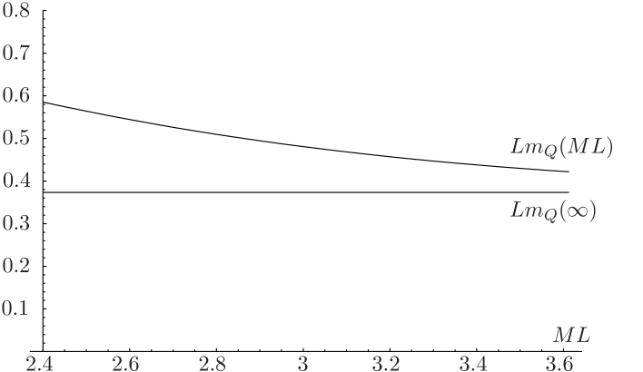
Figure 2: The mass of the left handed stop as a function of the localization parameter $ML$, compared with the same mass in the $ML\longrightarrow\infty$ limit.

4.1 Determination of the Fermi scale

With the inclusion of the tree level contribution from eq. (3), the minimum equation (5) reads

$$\frac{M_{Z}^{2}}{4}=-\delta V^{\prime}(v^{2})$$ (20)

which must be viewed as a relation between the compactification scale $1/L$ and the localization parameter $ML$. Fig. 3 shows

$$-L^{2}\delta V^{\prime}(v^{2})=-L^{2}\delta V^{\prime}_{\textrm{ew}}(v^{2})-L^{2}\delta V^{\prime}_{\textrm{top}}(v^{2};ML)$$ (21)

with the electroweak contribution given in eq. (7) and the top contribution from eq. (17) or (18).

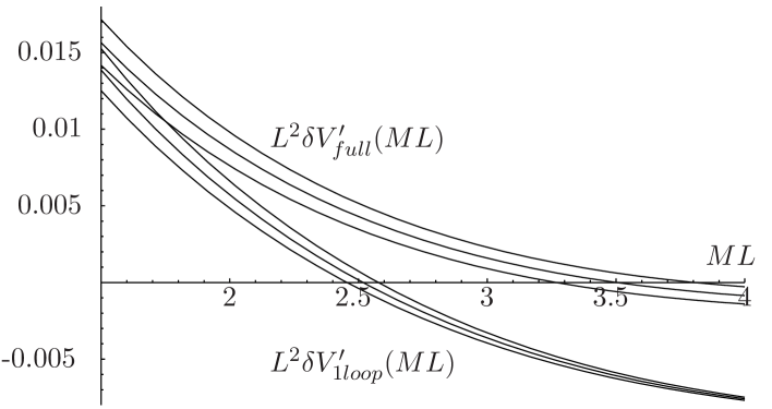
Figure 3: Slope of the full radiative Higgs potential, as discussed in the text, versus the top localization parameter $ML$, compared to the one loop approximation, for $m_{t}^{pole}=174.3\pm 5.1{\rm\mbox{ }GeV}$.

After rescaling by $1/L^{2}$, $\delta V^{\prime}(v^{2})$ has no significant residual dependence on $1/L$ in the region of interest, $1/L\geq 2\textrm{ TeV}$. For these values of $1/L$, it is $(M_{Z}L)^{2}\simeq 10^{-3}$, so that the one loop approximation to $\delta V_{\textrm{top}}^{\prime}$ is clearly inadequate. The flattening of $\delta V^{\prime}(v^{2})$ at $ML\simeq 3$, due to the partial cancellation between $\delta V_{\textrm{top}}^{\prime}$ and $\delta V_{\textrm{ew}}^{\prime}$, is important in reducing the tuning between $ML$ and $1/L$. Also in view of the uncertainties to be discussed below, this same flattening of $\delta V^{\prime}(v^{2})$ makes the precise relation between $ML$ and $1/L$ uncertain. This has little influence, however, on the relation between the Higgs mass and $1/L$, as we discuss shortly.

4.2 The Higgs mass as a function of $1/L$

With the inclusion of the correction in eq. (8) and of the top contribution from eq. (17), eq. (6) reads

$$m_{h}^{2} =M_{Z}^{2}\left[1-\frac{3}{4\,{\sqrt{2}}\,{\pi}^{2}}{G_{F}}\;{{m_{t}}}^{2}\;\log\left(\frac{m^{2}_{Q}(ML)m_{U}^{2}(ML)}{m_{t}^{4}}\right)\right]$$

$$+4\sqrt{2}G_{F}v^{4}\delta V_{\textrm{top}}^{\prime\prime}(v^{2};ML).$$ (22)

By means of the relation between $ML$ and $1/L$ as determined from the minimum equation, $m_{h}$ is plotted in Fig. 4 as function of $1/L$ only, for three different values of the pole top mass, $m_{t}^{pole}=174.3\pm 5.1\textrm{ GeV}$.

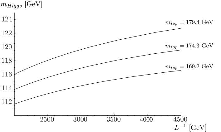
Figure 4: Higgs mass as function of $1/L$ for $m_{t}^{pole}=174.3\pm 5.1{\rm\mbox{ }GeV}$.

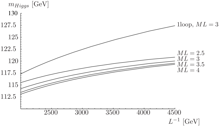
Figure 5: Higgs mass for $m_{t}^{pole}=174.3{\rm\mbox{ }GeV}$ at different fixed values of the top localization parameter. The result with the full Higgs potential is compared with the one only including the standard top correction at one loop.

In Figure 5 we show the band of values that would be obtained if $ML$ were not related to $1/L$ by the minimum equation (20), but kept fixed at values between 2 and 4. This shows that the precise relation between $ML$ and $1/L$ is almost irrelevant in order to determine the connection between $m_{h}$ and the compactification scale. In the same Fig. 5 we also compare the Higgs mass, calculated on the basis of eq. (4.2), with the one that would be obtained from a minimally improved lowest order formula

$$m_{h}^{2}(\textrm{naive})=M_{Z}^{2}+\frac{3\sqrt{2}}{4\pi}G_{F}m_{t}^{4}\log\left(\frac{m^{2}_{Q}(ML)m_{U}^{2}(ML)}{m_{t}^{4}}\right)$$ (23)

and $ML=2\div 4$. This comparison makes clear that the improved two loop potential is essential for a better determination of $m_{h}$.

4.3 Uncertainties

In this way one is naturally lead to the issue of the overall uncertainties on $m_{h}$, in particular on Fig. 4. We believe that the deviation from the localized approximation is properly accounted for by eqs. (17)-(18). The real question, then, is the validity of eqs. (3.2)-(3.2) with an exactly localized top. To this end, it is necessary to discuss the possible role of other operators than those in eq. (2). Among those operators, the potentially most important ones are the kinetic terms of the Higgs and the gauge multiplets localized on the boundaries. In the notation of eq. (1), the constants $z_{H}$, $z_{a}$ in

$$\delta{\cal L}=\delta(y)\left[z_{H}\int{\rm d}^{4}\theta\,H^{\dagger}e^{V}H+\sum_{a}\left(z_{a}\int{\rm d}^{2}\theta\,W^{(a)}_{\alpha}W^{(a)}_{\alpha}+{\rm h.c.}\right)\right]$$ (24)

with $a=SU(3),SU(2),U(1)$ and similar terms localized at $y=L$, have to be treated as additional parameters. For them we need an estimate or a natural assumption for their size. Since $H$ and $W^{(a)}_{\alpha}$ are 5D fields, their $z$-factors in eq. (24) have dimension of an inverse mass. Pure dimensional analysis leads to an estimate $z\sim 1/\Lambda$, where $\Lambda$ could either be the scale $\Lambda_{np}$ at which some of the couplings become non perturbative or a cutoff scale $\Lambda_{cutoff}\gtrsim\Lambda_{np}$ below which our 5D theory represents the low energy effective description of some more fundamental theory. By studying the evolution of the Yukawa couplings of the top and the bottom, localized at $y=0$ and $y=L$ respectively, one finds that $\Lambda_{np}L=6\div 10$ at $ML\simeq 3$ [4, 5]. For equal masses, (equal localization), of the quark hypermultiplets of the third generation, $M$, it is in fact $\lambda_{b}$ that becomes non perturbative first. To produce the physical top and bottom masses, both $\lambda_{t}$ and $\lambda_{b}$ depend on $ML$ and become comparable for $ML=2\div 2.5$, whereas for higher $ML$ $\lambda_{b}$ becomes progressively bigger.

Based on these considerations/assumptions, we take for the dimensionless $Z$-factors

$$Z\equiv\frac{z}{L}\lesssim(10\div 15)\%.$$ (25)

On the other hand the introduction of these $z$-factors affects the radiative Higgs potential or the radiative squark masses $m^{2}_{Q}$, $m_{U}^{2}$ only at quadratic order in the dimensionless $Z$’s. On this basis we expect that the calculations of the Higgs and squark masses are correct within a few %. A more critical quantity is $\delta V^{\prime}$, since the electroweak and the top contributions cancel quite accurately against each other and are renormalized by different factors $(1+{\cal O}(Z^{2}))$. As already mentioned in Sect. 4.1, although making uncertain the relation between $ML$ and $1/L$, this has little influence, however, on the relation between $m_{h}$ and $1/L$.

5 Lower values of the compactification scale

An interesting question is what happens for $1/L$ lower than $2\;{\rm\mbox{ }TeV}$. Below this value the Higgs mass gets nominally lower than the experimental bound. Had we drawn the same figure as Fig. 4 for lower $1/L$, $m_{h}$ would have reached values as low as $105{\rm\mbox{ }GeV}$ at $1/L\simeq 600{\rm\mbox{ }GeV}$ to grow again up to $\simeq 130{\rm\mbox{ }GeV}$ at $1/L\simeq 300{\rm\mbox{ }GeV}$. At the same time, $ML$ progressively decreases from about 2 at $1/L\simeq 2{\rm\mbox{ }TeV}$, to zero at the lowest value of $1/L\simeq 300{\rm\mbox{ }GeV}$, where one makes contact with the “Constrained Standard Model” of Ref. [5]. We do not show this plot because in the intermediate region of $1/L\approx 1{\rm\mbox{ }TeV}$ or $ML\simeq 1$, our calculation is not fully reliable: $\delta V_{\textrm{top}}^{1loop}$ does not clearly dominate over the 2 loop contribution, which, on the other hand, is only to be trusted for sufficiently large $ML$.

To make sense of the model at these lower values of $1/L$, one has also to make sure that the potential with two Higgs doublets, $h$ and $h_{c}$, does not get destabilized, given the absence of a bilinear term $hh^{c}$. This is possible, without introducing a FI term, by adding a small common mass, $|M_{H}L|\lesssim 0.1$ for the Higgs hypermultiplets.

A non zero $M_{H}$ does not affect the physical Higgs mass, through $V^{\prime\prime}$, but only the determination of the Fermi scale, via $V^{\prime}$. With an extra term $(-M_{H}L)$, present in the right hand side of eq. (21), $1/L$ is not tied anymore to $ML$, which can in turn vary in a range consistent with a moderate amount of fine tuning. The result of this is shown in Fig. 6. Different values of $ML$ are used, but always in such a way that no fine tuning occurs stronger than $10\%$ in the determination of $G_{F}^{-1/2}$. The rise in $m_{h}$ is due to the stronger influence, for low $ML$, of $\delta V_{\textrm{top}}^{\textrm{1loop}}$, a fact which has no correspondence in the MSSM [4, 5].

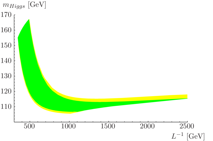
Figure 6: Expected range of Higgs masses with the inclusion of a hypermultiplet Higgs mass and a maximum fine tuning in the slope of the potential at $10\%$ level. The darker (lighter) area is for $m_{t}^{\textrm{pole}}=174.3$ ($174.3\pm 5.1$)

Taking into account the uncertainties mentioned above, a value of $m_{h}$ marginally consistent with the experimental lower bound of $114{\rm\mbox{ }GeV}$ cannot be excluded in the entire region of $1/L$. The existence of independent lower bounds on $1/L$ becomes then of relevance. This in turn crucially depends on the masses $M_{Q_{i}}$, $M_{L_{i}}$ for the quark and lepton hypermultiplets of the different generations, $i=1,2,3$ [2]. Depending on these masses, modifications of the Fermi constant [13] and/or Flavor Changing Neutral Currents effects [14] are possible by tree level exchanges of KK states of the gauge bosons. These effects, however, are minimized (made to vanish at tree level) by the choice $M_{L_{i}}=0$, $M_{Q_{i}}=M$. It is in fact possible that the most important constraint on $1/L$ comes from the electroweak $\rho$ parameter. Simple dimensional analysis shows that the correction to the $\rho$ parameter from the towers of top and bottom states scales as $\delta\rho=c\,v^{2}/\left(L^{2}\Lambda^{4}\right)$ with a dimensionless coefficient that could perhaps be as large as 30 [5]. Although this correction, at fixed $\Lambda L=6\div 10$, vanishes as $L^{2}$ for small $L$, a value of $1/L$ as large as $1{\rm\mbox{ }TeV}$ might be needed to suppress this $\delta\rho$ correction below the uncertainty of the observed value.

6 Spectrum

The most peculiar feature of the spectrum is the heaviness of gauginos–higgsinos with a mass $\pi/(2L)$. The lightest superpartner is therefore a squark or a slepton, most likely charged, which can be stable or practically stable if a small $U(1)_{R}$-breaking coupling is present. The first KK states corresponding to the SM particles are at $\pi/L$. The masses of the sfermions of charge $Q$ and hypercharge $Y$ are given by

$$m^{2}=m^{2}_{tree}+m^{2}_{rad}+Ym_{Z}^{2}-Qm_{W}^{2}$$ (26)

where $m_{tree}$ is the tree level mass, including the Yukawa contribution, and $m_{rad}$ is the one loop contribution, as in eq. 13. As seen in Sect. 4, both $m_{tree}$ and $m_{rad}$ depend upon the corresponding localization parameter $ML$. For $ML=0$, $m_{tree}=\pi/(2L)$ dominates and the sfermion becomes degenerate with the gauginos and the higgsinos. For $ML\gtrsim 1$, $m_{rad}$ dominates and rapidly approaches the localized limit where

$$m_{rad}(\widetilde{Q}) =(370{\rm\mbox{ }GeV})\frac{1}{L{\rm\mbox{ }TeV}}$$ (27a)

$$m_{rad}(\widetilde{U}) =(382{\rm\mbox{ }GeV})\frac{1}{L{\rm\mbox{ }TeV}}$$ (27b)

$$m_{rad}(\widetilde{D}) =(310{\rm\mbox{ }GeV})\frac{1}{L{\rm\mbox{ }TeV}}$$ (27c)

$$m_{rad}(\widetilde{L}) =(137{\rm\mbox{ }GeV})\frac{1}{L{\rm\mbox{ }TeV}}$$ (27d)

$$m_{rad}(\widetilde{E}) =(79{\rm\mbox{ }GeV})\frac{1}{L{\rm\mbox{ }TeV}}$$ (27e)

Up to the D-term effects in eq. (26), these are lower values for the sfermion masses.

As we have seen, the localization parameter of the third generation squarks is correlated with the compactification scale by EWSB. For $1/L\gtrsim 2{\rm\mbox{ }TeV}$, eq. (27a) gives the mass of the left handed stop and sbottom, split by $m_{tree}(\widetilde{t})=m_{t}$, whereas $\left(m_{rad}(\widetilde{U})^{2}+m_{t}^{2}\right)^{1/2}$ is the mass of the right-handed stop.

For lower values of $1/L$, if a tree level mass of the Higgs hypermultiplets is present (see Sect. 5), the third generation squarks can be progressively delocalized. In this case eqs. (27) give a lower bound, with the overall masses that can go up to $800{\rm\mbox{ }GeV}$ even for $1/L$ below $1{\rm\mbox{ }TeV}$.

Eqs. (26) and (27d) apply also to the masses of the scalars in the second Higgs hypermultiplet $H_{c}$, without a vev and with gauge couplings identical to those of a left-handed slepton multiplet. Not to undo EWSB, the Higgs hypermultiplets are always almost fully delocalized, $|M_{H}L|\leq 0.1$. Eq. (27d) is strictly valid for $1/L\gtrsim 2{\rm\mbox{ }TeV}$ and $m_{rad}(\widetilde{H})\gtrsim 270{\rm\mbox{ }GeV}$. For smaller values of $1/L$ a tree level Higgs mass can play a role and can raise the total mass of the charged and neutral scalars in $H_{c}$, relative to eq. (27d), by about $100{\rm\mbox{ }GeV}$ at $1/L\simeq 1{\rm\mbox{ }TeV}$.

7 Summary and conclusions

We have made an accurate calculation of the Higgs potential in a theory of EWSB triggered by the top Yukawa coupling, where supersymmetry is broken by boundary conditions on a fifth dimension. The calculability of the Higgs potential rests on the fact that supersymmetry breaking is described in terms of a single parameter, the length $L$ of the compactified extra dimension. This, in turn, is possible because the zeroth order spectrum has all the extra particles implied by supersymmetry and/or 5D Poincarè invariance at $\pi/(2L)$ or higher.

To define the phenomenology of this proposal, a central issue is the determination of the range of the compactification scale $1/L$. Although not with certainty, the ElectroWeak Precision Tests most likely want a value of $1/L$ above $1{\rm\mbox{ }TeV}$. This is a manifestation of the usual “little hierarchy problem”: the apparent need of a gap between the scale of physics that triggers EWSB and $G_{F}^{-1/2}$ or the Higgs mass, low according to the same EWPT. In the present case, the relation between $1/L$ and $G_{F}^{-1/2}$ is influenced by the level of localization of the top quark and, to a lesser extent, by a hypermultiplet Higgs mass. These are both unrenormalized supersymmetric parameters.

The two loop calculation of the Higgs potential shows that $1/L$ can go up to $4{\rm\mbox{ }TeV}$ without a significant amount of fine tuning and with the third generation Yukawa couplings maintaining perturbativity up to $\Lambda=(6\div 10)/L$. This is made possible by the localization of the top near the boundary of the 5th dimension where its Yukawa coupling is present. In this way the otherwise dominant one-loop top contribution to the curvature of the potential $V^{\prime}(v^{2})$ gets exponentially suppressed. Furthermore the two-loop diagrams involving the top Yukawa couplings in exactly localized approximation contribute to $V^{\prime}(v^{2})$ with a negative term that almost cancels the positive electroweak contribution, so that $L^{2}V^{\prime}(v^{2})=\mathcal{O}(10^{-3})$ for $ML\simeq 2.5\div 3.5$. This is the basis for allowing values of $1/L$ larger than $G_{F}^{-1/2}$ by about one order of magnitude.

To make sure that this is at all consistent with the phenomenological constraints, it is crucial to compare the expected Higgs mass with the current lower bound. To this purpose, with a reasonable assumption on the uncertainties induced by boundary $Z$-factors, it has been necessary to extend to two loop also the calculation of $V^{\prime\prime}(v^{2})$. For large values of $1/L=2\div 4{\rm\mbox{ }TeV}$, the Higgs mass is reduced with respect to the naive expectation and is in the $110\div 125{\rm\mbox{ }GeV}$ range. For lower values of $1/L$ the Higgs mass is more uncertain but can be above the experimental bound up to the lowest possible values of $1/L$.

The spectrum implied by this picture of supersymmetry and electroweak symmetry breaking has a few characteristic features. The first KK states corresponding to the SM particles are at $\pi/L$. Also all gauginos and higgsinos are heavy, with a mass at $\pi/(2L)$. Therefore the lightest superpartner is a sfermion, most likely charged, which can be stable or practically stable for collider experiments [2, 5]. Finally one also expects relatively light scalars, one charged and one neutral, belonging to the $H_{c}$ hypermultiplet, introduced to cancel the FI term. They are coupled to the gauge bosons as a lepton doublet but have unknown couplings to quarks and leptons.

Acknowledments

We thank P. Slavich for useful comments concerning the two loop corrections to the Higgs mass in the MSSM. This work has been partially supported by MIUR and by the EU under TMR contract HPRN-CT-2000-00148.

Appendix A The 2 loop contribution to the Higgs potential

In this appendix we give some details of the 2 loop contribution to the Higgs potential $\delta V_{\textrm{top}}^{\textrm{2 loop}}$.

At the 2-loop level there are two contributions. The first one comes from the expansion, in eq. (3.1), of the one loop corrections in eqs. (12) after expressing $m_{0,t}$, $m_{0,Q}$ and $m_{0,U}$ in terms of the renormalized masses $m_{t}$, $m_{Q}$ and $m_{U}$ respectively. The second contribution is a pure 2-loop correction and corresponds to the diagrams of Fig. 1 in terms of the top superfields $U,Q$, the Higgs superfield $H$ and the $SU(3)$ vector superfiled $V$. In localized approximation for $U$ and $Q$, only $V$ and $H$ are 5-dimensional superfields.

Defining

$$C(x)=x\coth(x)\hskip 56.9055ptT(x)=x\tanh(x)$$ (28)

the pure 2-loop gauge correction (arising from the diagrams (1)-b) is given by the following expression

$$V_{\textrm{2loop,gauge}}=4\,{{g_{s}}}^{2}\,\int \frac{d^{4}p}{(2\pi)^{4}}\frac{d^{4}q}{(2\pi)^{4}}\frac{T(qL)}{q^{2}}\times$$

$$\times \left[\frac{-2\,q^{2}}{\left({\left(p-q\right)}^{2}+{{m_{Q}}}^{2}\right)\,\left(p^{2}+{{m_{t}}}^{2}\right)}-\frac{2\,p^{2}}{\,\left({\left(p-q\right)}^{2}+{{m_{Q}}}^{2}\right)\,\left(p^{2}+{{m_{t}}}^{2}\right)}\right.$$

$$+\frac{2\,{\left(p-q\right)}^{2}}{\,\left({\left(p-q\right)}^{2}+{{m_{Q}}}^{2}\right)\,\left(p^{2}+{{m_{t}}}^{2}\right)}-\frac{2\,q^{2}}{\left(p^{2}+{{m_{t}}}^{2}\right)\,\left({\left(p-q\right)}^{2}+{{m_{U}}}^{2}\right)}$$

$$-\left.\frac{2\,p^{2}}{\,\left(p^{2}+{{m_{t}}}^{2}\right)\,\left({\left(p-q\right)}^{2}+{{m_{U}}}^{2}\right)}+\frac{2\,{\left(p-q\right)}^{2}}{\,\left(p^{2}+{{m_{t}}}^{2}\right)\,\left({\left(p-q\right)}^{2}+{{m_{U}}}^{2}\right)}\right]$$

$$+4\,{{g_{s}}}^{2}\,\int \frac{d^{4}p}{(2\pi)^{4}}\frac{d^{4}q}{(2\pi)^{4}}\frac{C(qL)}{q^{2}}\times$$

$$\times \left[\frac{4}{\,\left({\left(p-q\right)}^{2}+{{m_{Q}}}^{2}\right)}+\frac{q^{2}}{\left(p^{2}+{{m_{Q}}}^{2}\right)\,\left({\left(p-q\right)}^{2}+{{m_{Q}}}^{2}\right)}\right.$$

$$-\frac{p^{2}}{\,\left(p^{2}+{{m_{Q}}}^{2}\right)\,\left({\left(p-q\right)}^{2}+{{m_{Q}}}^{2}\right)}-\frac{{\left(p-q\right)}^{2}}{\,\left(p^{2}+{{m_{Q}}}^{2}\right)\,\left({\left(p-q\right)}^{2}+{{m_{Q}}}^{2}\right)}$$

$$+\frac{2\,q^{2}}{\left(p^{2}+{{m_{t}}}^{2}\right)\,\left({\left(p-q\right)}^{2}+{{m_{t}}}^{2}\right)}-\frac{2\,p^{2}}{\,\left(p^{2}+{{m_{t}}}^{2}\right)\,\left({\left(p-q\right)}^{2}+{{m_{t}}}^{2}\right)}$$

$$-\frac{2\,{\left(p-q\right)}^{2}}{\,\left(p^{2}+{{m_{t}}}^{2}\right)\,\left({\left(p-q\right)}^{2}+{{m_{t}}}^{2}\right)}-\frac{8\,{{m_{t}}}^{2}}{\,\left(p^{2}+{{m_{t}}}^{2}\right)\,\left({\left(p-q\right)}^{2}+{{m_{t}}}^{2}\right)}$$

$$+\frac{4}{\,\left(p^{2}+{{m_{U}}}^{2}\right)}+\frac{q^{2}}{\left(p^{2}+{{m_{U}}}^{2}\right)\,\left({\left(p-q\right)}^{2}+{{m_{U}}}^{2}\right)}$$

$$-\left.\frac{p^{2}}{\,\left(p^{2}+{{m_{U}}}^{2}\right)\,\left({\left(p-q\right)}^{2}+{{m_{U}}}^{2}\right)}-\frac{{\left(p-q\right)}^{2}}{\,\left(p^{2}+{{m_{U}}}^{2}\right)\,\left({\left(p-q\right)}^{2}+{{m_{U}}}^{2}\right)}\right]$$

Analogously the pure 2-loop Yukawa correction (arising from the diagrams (1)-a) is given by the following expression

$$V_{\textrm{2loop,Yuk.}}=3\,{{y_{t}}}^{2}\int \frac{d^{4}p}{(2\pi)^{4}}\frac{d^{4}q}{(2\pi)^{4}}\frac{T(qL)}{q^{2}}\times$$

$$\times \left[\frac{{\left(p-q\right)}^{2}}{\left({\left(p-q\right)}^{2}+{{m_{Q}}}^{2}\right)\,\left(p^{2}+{{m_{t}}}^{2}\right)}-\frac{p^{2}}{\left({\left(p-q\right)}^{2}+{{m_{Q}}}^{2}\right)\,\left(p^{2}+{{m_{t}}}^{2}\right)}\right.$$

$$-\frac{q^{2}}{\left({\left(p-q\right)}^{2}+{{m_{Q}}}^{2}\right)\,\left(p^{2}+{{m_{t}}}^{2}\right)}-\frac{p^{2}}{\left({\left(p-q\right)}^{2}+{{m_{Q}}}^{2}-{{m_{t}}}^{2}\right)\,\left(p^{2}+{{m_{t}}}^{2}\right)}$$

$$+\frac{{\left(p-q\right)}^{2}}{\left({\left(p-q\right)}^{2}+{{m_{Q}}}^{2}-{{m_{t}}}^{2}\right)\,\left(p^{2}+{{m_{t}}}^{2}\right)}-\frac{q^{2}}{\left({\left(p-q\right)}^{2}+{{m_{Q}}}^{2}-{{m_{t}}}^{2}\right)\,\left(p^{2}+{{m_{t}}}^{2}\right)}$$

$$-\frac{1}{p^{2}+{{m_{U}}}^{2}}+\frac{p^{2}}{{\left(p-q\right)}^{2}\,\left(p^{2}+{{m_{U}}}^{2}\right)}-\frac{q^{2}}{{\left(p-q\right)}^{2}\,\left(p^{2}+{{m_{U}}}^{2}\right)}$$

$$+\frac{p^{2}}{\left({\left(p-q\right)}^{2}+{{m_{t}}}^{2}\right)\,\left(p^{2}+{{m_{U}}}^{2}\right)}-\frac{{\left(p-q\right)}^{2}}{\left({\left(p-q\right)}^{2}+{{m_{t}}}^{2}\right)\,\left(p^{2}+{{m_{U}}}^{2}\right)}$$

$$-\left.\frac{q^{2}}{\left({\left(p-q\right)}^{2}+{{m_{t}}}^{2}\right)\,\left(p^{2}+{{m_{U}}}^{2}\right)}\right]$$

$$\hskip 42.67912pt+3\,{{y_{t}}}^{2}\int \frac{d^{4}p}{(2\pi)^{4}}\frac{d^{4}q}{(2\pi)^{4}}\frac{C(qL)}{q^{2}}\times$$

$$\times \left[\frac{p^{2}}{\left(p^{2}+{{m_{Q}}}^{2}\right)\,\left({\left(p-q\right)}^{2}+{{m_{Q}}}^{2}\right)}+\frac{{{m_{Q}}}^{2}-{{m_{t}}}^{2}}{\left(p^{2}+{{m_{Q}}}^{2}\right)\,\left({\left(p-q\right)}^{2}+{{m_{Q}}}^{2}\right)}\right.$$

$$+\frac{p^{2}}{\left(p^{2}+{{m_{Q}}}^{2}\right)\,\left({\left(p-q\right)}^{2}+{{m_{Q}}}^{2}-{{m_{t}}}^{2}\right)}+\frac{{{m_{Q}}}^{2}-{{m_{t}}}^{2}}{\left(p^{2}+{{m_{Q}}}^{2}\right)\,\left({\left(p-q\right)}^{2}+{{m_{Q}}}^{2}-{{m_{t}}}^{2}\right)}$$

$$-\frac{1}{p^{2}+{{m_{t}}}^{2}}-\frac{p^{2}}{{\left(p-q\right)}^{2}\,\left(p^{2}+{{m_{t}}}^{2}\right)}+\frac{q^{2}}{{\left(p-q\right)}^{2}\,\left(p^{2}+{{m_{t}}}^{2}\right)}$$

$$-\frac{p^{2}}{\left(p^{2}+{{m_{t}}}^{2}\right)\,\left({\left(p-q\right)}^{2}+{{m_{t}}}^{2}\right)}-\frac{{\left(p-q\right)}^{2}}{\left(p^{2}+{{m_{t}}}^{2}\right)\,\left({\left(p-q\right)}^{2}+{{m_{t}}}^{2}\right)}$$

$$+\frac{q^{2}}{\left(p^{2}+{{m_{t}}}^{2}\right)\,\left({\left(p-q\right)}^{2}+{{m_{t}}}^{2}\right)}+\frac{1}{p^{2}+{{m_{U}}}^{2}}$$

$$+\frac{q^{2}}{\left({\left(p-q\right)}^{2}+{{m_{Q}}}^{2}\right)\,\left(p^{2}+{{m_{U}}}^{2}\right)}+\frac{q^{2}}{\left({\left(p-q\right)}^{2}+{{m_{Q}}}^{2}-{{m_{t}}}^{2}\right)\,\left(p^{2}+{{m_{U}}}^{2}\right)}$$

$$+\left.\frac{{\left(p-q\right)}^{2}}{\left(p^{2}+{{m_{U}}}^{2}\right)\,\left({\left(p-q\right)}^{2}+{{m_{U}}}^{2}\right)}+\frac{-{{m_{t}}}^{2}+{{m_{U}}}^{2}}{\left(p^{2}+{{m_{U}}}^{2}\right)\,\left({\left(p-q\right)}^{2}+{{m_{U}}}^{2}\right)}\right]\,$$

In the 2-loop potential, we have used the physical (renormalized) quantities $m_{t}^{2},\,m_{U}^{2},\,m_{Q}^{2}$ because the corrections are of higher order. When one takes the derivatives of the potential one has to remember that

$$v^{2}\frac{\textrm{d}}{\textrm{d}v^{2}}=m_{t}^{2}\left(\frac{\partial}{\partial m_{t}^{2}}+\frac{\partial}{\partial m_{U}^{2}}+\frac{\partial}{\partial m^{2}_{Q}}\right)$$ (29)

because all the 3 masses depend on the VEV $v$.

The integrals in $p$ can be performed analitically. Then, to get the leading logarithmic contributions as $L\rightarrow 0$, one can use the asymptotic behaviour of the $q$-integrand functions. In this way one gets the results given in eqs. (3.2)-(3.2).

Appendix B 1-loop Renormalization functions at order $\alpha_{t}$, $\alpha_{s}$

In order to compute the physical masses in Eqs. (12a)-(12c), the one loop corrections ${\cal O}(\alpha_{t},\alpha_{s})$ to the propagators of the $U$,$Q$-multiplets and to the Yukawa vertex are needed.

At order $\alpha_{t}$ the propagators of the top, stop and auxiliary field get corrected from the exchange of the Higgs supermultiplet H and a U (or Q) quark multiplet.

These corrections can be parameterized as usual

where we have used a superfield notation in the loop and an Euclidean external momentum $p$. The Yukawa vertex receives no direct correction at order $\alpha_{t}$ because of the non-renormalization properties of the superpotential.

All the quantities defined above, to the order $y_{t}^{2}$, are given by

$$B_{F}^{U}(0) =-y_{t}^{2}\int\frac{d^{4}q}{(2\pi)^{4}}C\left(qL\right)\left[\frac{1}{q^{2}+m^{2}_{Q}+m_{t}^{2}}+\frac{1}{q^{2}+m^{2}_{Q}}\right]$$ (30a)

$$B_{F}^{Q}(0) =-y_{t}^{2}\int\frac{d^{4}q}{(2\pi)^{4}}C\left(qL\right)\left[\frac{1}{q^{2}+m^{2}_{Q}+m_{t}^{2}}\right]$$ (30b)

$$B_{\varphi}^{Q}(0) =y_{t}^{2}\int\frac{d^{4}q}{(2\pi)^{4}}\frac{1}{q^{2}}\left\{C\left(qL\right)\left[\frac{q^{2}(m_{t}^{2}+m^{2}_{U})}{(q^{2}+m_{t}^{2}+m^{2}_{U})^{3}}-\frac{m_{t}^{2}(m_{t}^{2}+m^{2}_{Q})}{(q^{2}+m_{t}^{2}+m^{2}_{Q})^{3}}\right]\right.$$

$$\hskip 71.13188pt\left.-T\left(qL\right)\left[\frac{q^{4}+3m_{t}^{2}q^{2}}{(q^{2}+m_{t}^{2})^{3}}\right]\right\}$$ (30c)

$$B_{\varphi}^{U}(0) =y_{t}^{2}\int\frac{d^{4}q}{(2\pi)^{4}}\frac{1}{q^{2}}\left\{C\left(qL\right)\left[\frac{q^{2}(m_{t}^{2}+m^{2}_{Q})}{(q^{2}+m_{t}^{2}+m^{2}_{Q})^{3}}-\frac{m_{t}^{2}(m_{t}^{2}+m^{2}_{U})}{(q^{2}+m_{t}^{2}+m^{2}_{U})^{3}}+\frac{q^{2}m^{2}_{Q}}{(q^{2}+m^{2}_{Q})^{3}}\right]\right.$$

$$\hskip 71.13188pt\left.-T\left(qL\right)\left[\frac{q^{4}+3m_{t}^{2}q^{2}}{(q^{2}+m_{t}^{2})^{3}}+\frac{1}{q^{2}}\right]\right\}$$ (30d)

$$B_{\psi}^{Q}(0) =-\frac{y_{t}^{2}}{2}\int\frac{d^{4}q}{(2\pi)^{4}}\frac{1}{q^{2}}\left\{C\left(qL\right)\frac{q^{2}+2m_{t}^{2}}{(q^{2}+m_{t}^{2})^{2}}+T\left(qL\right)\frac{q^{2}}{(q^{2}+m^{2}_{U}+m_{t}^{2})^{2}}\right\}$$ (30e)

$$B_{\psi}^{U}(0) =-\frac{y_{t}^{2}}{2}\int\frac{d^{4}q}{(2\pi)^{4}}\frac{1}{q^{2}}\left\{C\left(qL\right)\left[\frac{q^{2}+2m_{t}^{2}}{(q^{2}+m_{t}^{2})^{2}}+\frac{1}{q^{2}}\right]\right.$$

$$\hskip 71.13188pt\left.-T\left(qL\right)\left[\frac{q^{2}}{(q^{2}+m^{2}_{Q}+m_{t}^{2})^{2}}+\frac{q^{2}}{(q^{2}+m^{2}_{Q})^{2}}\right]\right\}$$ (30f)

$$\delta m^{2}_{Q} =y_{t}^{2}\int\frac{d^{4}q}{(2\pi)^{4}}\frac{1}{q^{2}}\left\{C\left(qL\right)\left[\frac{q^{2}+m^{2}_{Q}}{q^{2}+m^{2}_{Q}+m_{t}^{2}}+\frac{q^{2}}{q^{2}+m_{0,u}^{2}+m_{t}^{2}}\right]-T\left(qL\right)\frac{2q^{2}}{q^{2}+m_{t}^{2}}\right\}$$ (30g)

$$\delta m^{2}_{U} =y_{t}^{2}\int\frac{d^{4}q}{(2\pi)^{4}}\frac{1}{q^{2}}\left\{C\left(qL\right)\left[\frac{q^{2}+m^{2}_{U}}{q^{2}+m^{2}_{U}+m_{t}^{2}}+1+\frac{q^{2}}{q^{2}+m_{q}^{2}+m_{t}^{2}}+\frac{q^{2}}{q^{2}+m^{2}_{Q}}\right]\right.$$

$$\hskip 71.13188pt\left.-T\left(qL\right)\left[\frac{2q^{2}}{q^{2}+m_{t}^{2}}+2\right]\right\}$$ (30h)

where the functions $C\left(x\right)$ and $T\left(x\right)$ are given in (28). The integration over the momentum $q$ has to be performed on Euclidean space.

At order $\alpha_{s}$ only the propagators of the top and the stops, but not of their auxiliary fields, get corrected from the exchange of the $SU(3)$ gauge supermultiplet $V$ and of a quark multiplet. Performing the calculation in the Wess-Zumino gauge there is also a direct correction to the Yukawa interaction, so that

Parameterizing these $g_{s}^{2}$-corrections as in the $y_{t}^{2}$ case, one has

$$B_{\varphi}^{i}(0) =\frac{8}{3}g_{s}^{2}\int\frac{d^{4}q}{(2\pi)^{4}}\frac{1}{q^{2}}\left\{C\left(qL\right)\frac{q^{2}+2(m_{i}^{2}+m_{t}^{2})}{(q^{2}+m_{i}^{2}+m_{t}^{2})^{2}}-T\left(qL\right)\frac{q^{4}+3q^{2}m_{t}^{2}}{(q^{2}+m_{t}^{2})^{3}}\right\}$$ (31a)

$$B_{\psi}^{i}(0) =-\frac{4}{3}g_{s}^{2}\int\frac{d^{4}q}{(2\pi)^{4}}\frac{1}{q^{2}}\left\{C\left(qL\right)\frac{q^{2}+2m_{t}^{2}}{(q^{2}+m_{t}^{2})^{2}}+T\left(qL\right)\frac{q^{2}}{(q^{2}+m_{i}^{2}+m_{t}^{2})^{2}}\right\}$$ (31b)

$$\delta m^{2}_{i} =\frac{16}{3}g_{s}^{2}\int\frac{d^{4}q}{(2\pi)^{4}}\frac{1}{q^{2}}\left\{C\left(qL\right)-T\left(qL\right)\frac{q^{2}}{q^{2}+m_{t}^{2}}\right\}$$ (31c)

$$Z_{y_{t}}(0) =\frac{16}{3}g_{s}^{2}\int\frac{d^{4}q}{(2\pi)^{4}}\frac{1}{q^{2}}C\left(qL\right)\frac{q^{2}}{(q^{2}+m_{t}^{2})^{2}}$$ (31d)

where $i=U,Q$.

All the quantities defined above are regular in the IR except $B_{\psi}^{U}$. Because we are interested only in the logarithmic contributions to $\delta V^{\prime\prime}(v^{2})$, we can evaluate the $B_{\varphi}$ and $B_{F}$ functions at vanishing external momentum. Instead, the functions $B_{\psi}$ and $Z_{y_{t}}$, involved in eq. (12a), have to be evaluated at $p^{2}=m_{t}^{2}$. Given their expressions at $p^{2}=0$ one has to add

$$B_{\psi}^{Q}\left(m_{t}^{2}\right)-B_{\psi}^{Q}\left(0\right) =\frac{\alpha_{s}}{6\pi}+\frac{\alpha_{t}}{16\pi}$$ (32)

$$B_{\psi}^{U}\left(m_{t}^{2}\right)-B_{\psi}^{U}\left(0\right) =\frac{\alpha_{s}}{6\pi}+\frac{\alpha_{t}}{16\pi}+4\pi\alpha_{t}\int\frac{d^{4}q}{(2\pi)^{4}}\left[\right.\frac{1}{2\,q^{4}}+\frac{4\,\log(\frac{2\,q}{{m_{t}}+{\sqrt{4\,q^{2}+{{m_{t}}}^{2}}}})}{{m_{t}}\,{\left(4\,q^{2}+{{m_{t}}}^{2}\right)}^{\frac{3}{2}}}$$

$$\hskip 133.72786pt-\frac{1}{q^{2}\,\left(4\,q^{2}+{{m_{t}}}^{2}\right)}\left.\right]$$ (33)

$$Z_{y_{t}}\left(m_{t}^{2}\right)-Z_{y_{t}}\left(0\right) =\frac{4\alpha_{s}}{3\pi}\left(2-3\log 2\right)$$ (34)

Note that the IR divergence in (33) cancels the one in $B_{\psi}^{U}(0)$.

References

• [1] I. Antoniadis, Phys. Lett. B 246 (1990) 377;
I. Antoniadis, C. Munoz, M. Quiros, Nucl. Phys. B 397 (1993) 515 [hep-ph/9211309];
A. Delgado, A. Pomarol, M. Quiros, Phys. Rev. D 60 (1999) 095008 [hep-ph/9812489];
• [2] R. Barbieri, L. J. Hall, G. Marandella, Y. Nomura, T. Okui, S. J. Oliver and M. Papucci, arXiv:hep-ph/0208153.
• [3] D. Marti and A. Pomarol, Phys. Rev. D 66, 125005 (2002) [arXiv:hep-ph/0205034].
• [4] R. Barbieri, G. Marandella and M. Papucci, Phys. Rev. D 66, 095003 (2002) [arXiv:hep-ph/0205280].
• [5] R. Barbieri, L. J. Hall and Y. Nomura, Phys. Rev. D 63, 105007 (2001) [arXiv:hep-ph/0011311].
• [6] J. Scherk and J. H. Schwarz, Phys. Lett. B 82, 60 (1979); Nucl. Phys. B 153, 61 (1979).
• [7] D. M. Ghilencea, S. Groot Nibbelink and H. P. Nilles, Nucl. Phys. B 619, 385 (2001) [arXiv:hep-th/0108184].
• [8] R. Barbieri, R. Contino, P. Creminelli, R. Rattazzi and C. A. Scrucca, Phys. Rev. D 66, 024025 (2002) [arXiv:hep-th/0203039].
• [9] I. Antoniadis, S. Dimopoulos, A. Pomarol and M. Quiros, Nucl. Phys. B 544, 503 (1999) [arXiv:hep-ph/9810410].
• [10] A. Brignole, Phys. Lett. B 281, 284 (1992).
• [11] A. Delgado, A. Pomarol and M. Quiros, Ref. [1]
• [12] R. Hempfling and A. H. Hoang, Phys. Lett. B 331, 99 (1994) [arXiv:hep-ph/9401219].
• [13] A. Strumia, Phys. Lett. B 466, 107 (1999) [arXiv:hep-ph/9906266].
• [14] A. Delgado, A. Pomarol and M. Quiros, JHEP 0001, 030 (2000) [arXiv:hep-ph/9911252].