The density distribution in the Earth along the CERN-Pyhäsalmi baseline and its effect on neutrino oscillations

Abstract

We study the beamline properties of a long baseline neutrino- oscillation experiment from CERN to the Pyhäsalmi Mine in Finland. We obtain the real density profile for this particular neutrino oscillation beamline by applying the geophysical data. The effects of the matter density to neutrino oscillations are considered. Also we compare the realistic density profile with that acquired from the PREM model.

1 Introduction

A future step towards a better understanding of neutrino properties is to build long-baseline neutrino-oscillation experiments. One such possibility could be to aim a neutrino beam from a proposed CERN Neutrino Factory[1] to the Pyhäsalmi Mine in Finland 2288 km away. The Neutrino Factory and target station could be operational after the year 2010.

The oscillation probability depends on the density of the medium as well as the intrinsic mixing parameters. The purpose of this study is to compile a realistic density profile along the CERN-Pyhäsalmi neutrino baseline and estimate its effect on the neutrino oscillations.

2 Compilation of the density distribution along the baseline

2.1 The geographical position of the baseline

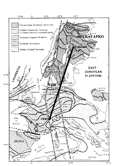
Figure 1: Location of the CERN-Pyhäsalmi baseline (solid black line) on the map of main tectonic elements of Western Europe[4]. The location of the EGT in the swathe between the two broad lines.

The neutrino baseline starts at $46^{\circ}$N $15^{\prime}$ $22.93^{\prime\prime}$, $06^{\circ}$E $03^{\prime}$ $01.10^{\prime\prime}$, $+450$ m above sea level, and ends at $63^{\circ}$N $39^{\prime}$ $34.74^{\prime\prime}$, $26^{\circ}$E $02^{\prime}$ $29.94^{\prime\prime}$, $-1345$ m. Its total length is $2288$ km. The geographical position of the baseline and its penetration depth were calculated using the geocentric Cartesian coordinate system and then transformed to the geographical coordinates and depth with respect to the WGS-84 ellipsoid [2] using the transformation equations in [3]. The location of the baseline is shown on the simplified tectonic map of Europe (Fig. 1). The baseline goes mainly through the lithosphere (the Earth’s crust and the uppermost part of the Earth’s mantle) and crosses the main geological structures and boundaries of the Europe. Its deepest point (103.81 km) is located below the so-called Trans-European Suture Zone (TESZ). Thus, the density variations along the line can be due to different thickness of the crust and different density of the crust and lithospheric mantle within various tectonic units. Another affecting factor is the depth to the boundary that separates the non-convecting lithospheric mantle from partially molten convecting and less dense asthenosphere. This information can be obtained from results of recent lithospheric studies in Europe.

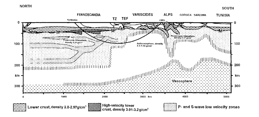
Figure 2: A sketch demonstrating the location of the CERN-Pyhäsalmi baseline on the composite cross-section of the lithopshere along the EGT [4] (solid black line). The depth to the lithosphere-asthenosphere boundary beneath the Trans-European Suture Zone is modified in accordance with the S-wave velocity model in [6]. M, Moho boundary; TZ Tornquist Zone; TEF, Trans-European Fault.

As seen from Fig. 1, the large part of the baseline is located within the study area of the European Geotraverse project (EGT). The EGT was a $4600$ km long and $200-300$ km wide lithospheric transect across Europe from Norway to Tunisia. The multinational, multidisciplinary research resulted in a comprehensive cross-section of the European lithosphere to the depth of $450$ km [4]. It revealed a significant contrast between the thickness and structure of the lithosphere of younger western Europe (less than $90$ km) and the old cold lithosphere of Fennoscandia and eastern Europe (more than $160$ km), occurring beneath the TESZ (Fig. 2). Later, the more detailed information about the lithosphere-asthenosphere boundary beneath the TESZ was obtained within the seismological EUROPROBE/TOR project [5][6].

In Finland, the CERN-Pyhäsalmi baseline is located within the study area of the EUROPROBE/SVEKALAPKO project [7]. As a part of the project, the 3D density model of the SVEKALAPKO area on a $2$ km $\times$ $2$ km $\times$ $2$ km rectangular grid down to the depth of $70$ km was obtained [8].

Thus, the abundant geophysical information about structure of the crust and upper mantle obtained within three large geoscientific projects in Europe mentioned above (e.g. EGT, TOR, SVEKALAPKO) allows us to compile a realistic density profile for the CERN-Pyhäsalmi baseline.

2.2 Composition and density of the continental crust and the lithospheric mantle

The thickness of the crust in Europe varies from $26$ km in its western part to 65 km beneath the Fennoscandia. The most abundant elements in the continental crust are O (46.4 wt$\%$), Si (28.15 wt$\%$), Al (8.23 wt$\%$), Fe (5.63 wt$\%$), Mg (2.33 wt$\%$), Ca (4.15 wt$\%$), Na (2.36 wt$\%$) and K (2.09 wt$\%$) [9], occuring in the Earth in the form of various silicate minerals. The density in the continental crust generally increases with depth due to the lithostatic pressure resulting in rock compaction and also due to decrease of the content of SiO₂ in the rock-forming minerals of lower crustal rocks. The strongest density contrasts in the crust exist between the sedimentary cover and the bedrock and also at the so-called Mochorovichich boundary (Moho boundary) separating the crust from the mantle.

The major part of the baseline is located within the upper $100$ km of the Earth’s litospheric mantle. The physical properties and composition of it are known from geophysical studies and from direct measurements on samples of mantle rocks that have been overthrusted or exhumed to the surface by various tectonic and magmatic processes. The main elements in the upper mantle are Fe, Mg, Si and O. The main rock forming minerals for upper mantle rocks (peridotites) are olivine ((Mg,Fe)₂SiO₂), orthopyroxene ((Mg,Fe)SiO₂), clinopyroxene ((Ca,Na)(Mg,Fe,Al, Cr,Ti)(Si,Al)₂O₆) and spinel (MgAl₂O₄). It is believed that the continental lithospheric mantle has undergone significant melting through geological time and is depleted in such components as Fe, Al, Ca and Ti. As a result, the density of the continental lithospheric mantle generally depends on the tectonothermal age: younger lithospheric mantle is less depleted and hence is denser. The conversion from fertile to depleted mantle is expressed by a decrease in clinopyroxene and orthopyroxene and relative increase in olivine, and also by an increase of Mg content. That is why the lithospheric mantle beneath the young Phanerosoic Western Europe has the average density of $3.37$ g$/$cm³, while the older (Proterozoic) mantle beneath the Fennoscandian Schield is less dense ($3.34$ g$/$cm³) [10].

In comparison to the lithospheric mantle, the asthenosphere is fertile and chemically more homogeneous because of convection. The density of the asthenosphere is less than that of the lithospheric mantle and depends mainly on the density and content of partially molten material (tholeitic basalt) [11].

The amount of partial melt in the asthenosphere can be estimated from the stability condition for the olivine-molten basalt mixtures. They are mechanically stable only in the case when the melt is concentrated within isolated, non-connected inclusions(pockets). The theoretical modelling of elastic and electrical properties of such mixtures[12] demonstrated that in some cases only $5\%$ of melt inclusions is enough to form a perfectly interconnected network. This value (less than $5\%$) is in agreement with estimates obtained by teleseismic tomography studies [13]. Thus, if the melt content is less than $5\%$, and the density of the molten basalt under upper mantle pressure-temperature conditions is $2.72$ g$/$cm³ [14], then the lithosphere-asthenosphere density contrast is less than $0.04$ g$/$cm³.

The lithosphere-asthenosphere density contrast beneath the TESZ can be roughly estimated also from the S-wave velocity ($V_{s}$) model in [6]. In accordance with it, the $V_{s}$ in the mantle lithosphere is $4.57$ km$/$s, while the $V_{s}$ in the asthenosphere is $4.36$ km$/$s. Using the scaling factor relating decrease in $V_{s}$ to the decrease in density, that is equal to $0.05$ at a depth of about $100$ km [15], the asthenophere density beneath the TESZ is $3.34$ g$/$cm³.

These estimates of the asthenosphere density agree with the results of regional (medium-wavelength and long-wavelength) gravity studies in Europe ($3.2-3.33$ g$/$cm³)[16]. Summarising all the data about the density in the asthenosphere cited above, we can conclude that the range of possible values of the asthenosphere density for Western Europe is $3.2-3.34$ g$/$cm³.

2.3 Geological setting and density values along the baseline

From $0$ to $175$ km the baseline goes through the Earth crust beneath the Jura Mountains, Molasse Basin and the Upper Rhine Graben. The thickness of the crust here is $30-28$ km [17]. The first $21$ km of the line are located within the sedimentary cover that is $3300-3400$ m thick[18]. The density within the sedimentary cover composed of limestones, sandstones and shales gradually increases with depth from $2.4$ to $2.6$ g$/$cm³.

The next portion of the line ($22-175$ km) goes through the upper($22-71$ km), middle ($72-119$ km) and lower crystalline crust ($120-175$ km) with the densities of $2.7-2.73$ g$/$cm³, $2.8-2.87$ g$/$cm³ and $2.96-2.97$ g$/$cm³, respectively. The thickness of the layers and their density were taken from the 3-D gravity studies[19][20].

The next part of the baseline ($175-732$ km) goes through the Palaeosoic lithospheric mantle ($3.37$ g$/$cm³). Basing on studies by [20][21] we assumed no upwelling asthenosphere beneath the Upper Rhine Graben ($175-430$ km). Thus, the baseline goes through the uprising asthenosphere only at $732-1019$ km. As it was shown in previous Chapter, the density of the asthenosphere here can be $3.20-3.34$ g$/$cm³. The lithosphere-asthenosphere boundary along the baseline was estimated in accordance with the lithosphere thickness map[22] and from the model[6], with the accuracy of $50$ km.

From $1020$ to $1956$ km the baseline is located within the Proterozoic lithospheric mantle ($3.34$ g$/$cm³), then it returns to the crust at a depth of $52.01$ km. The density values along the final part of the baseline ($1957-2288$ km) were taken from the 3-D density model of the SVEKALAPKO area[8]. The crust in this part of Finland consists of four major layers: the upper crust($2.73-2.81$ g$/$cm³), the middle crust($2.86-2.89$ g$/$cm³), the lower crust($2.86-2.89$ g$/$cm³) and so-called high-velocity lower crust($3.01-3.2$ g$/$cm³). The density values along the baseline are summarised in Figure 4.

3 Neutrino matter oscillations along the baseline

Next we will discuss the effect of the realistic CERN-Pyhäsalmi density profile to neutrino-oscillations. In a general three flavour framework the distance evolution equation of the neutrino flavour states can be written as[23]

$$i{\textrm{d}\over\textrm{d}x}\pmatrix{\nu_{e}\cr\nu_{\mu}\cr\nu_{\tau}}=\left({1\over 2E}U{M}^{2}U^{\dagger}+\pmatrix{\Delta V&0&0\cr 0&0&0\cr 0&0&0}\right)\times\pmatrix{\nu_{e}\cr\nu_{\mu}\cr\nu_{\tau}}$$ (1)

and we use the PDG endorsed parametrization[24] for the unitary mixing matrix $U$. The potential term $\Delta V=\pm\sqrt{2}G_{F}Y_{e}\rho$ arises from the coherent forward charged-current scatterings of electron neutrinos from the matter electrons. Throughout this paper we assume $Y_{e}=0.5$, because of the crust and mantle material content, which is mainly Si and O. We solve the equation (1) numerically by using a fourth order Runge-Kutta -algorithm.

At energies relevant to a neutrino factory beam (above $1$ GeV), the $\nu_{e}\rightarrow\nu_{\mu}$ -oscillations are governed mainly by the mixing angle $\theta_{13}$ and the mass squared difference $\delta m_{31}^{2}\approx\delta m_{32}^{2}$. For typical values of $\delta m_{31}^{2}=+3.0\cdot 10^{-3}\textrm{ eV}^{2}$, $\theta_{13}=0.1$ and density $\rho\approx 3.3$ g cm^-3, the matter resonance energy in the leading approximation[25] is about $\sim 11$ GeV, but the distance $2288$ km is much smaller than the corresponding oscillation lenght ($L_{osc}\sim 45000$ km) and therefore no total resonance conversion can happen. Our simulations show that the muon neutrino appearance probability at the first oscillation maximum ${E\sim 5}$ GeV is enhanced by about a factor of two compared to the appearance probability in vacuum. For a negative sign of $\delta m_{31}^{2}$, corresponding to the inverted mass hierarchy, the appearance probability is suppressed by about a factor of two. For $\overline{\nu}_{e}\rightarrow\overline{\nu}_{\mu}$-oscillations the situation is opposite (shown in Figure 3).

Figure 3: An example of muon neutrino and antineutrino appearance probabilities for different energies and mass hierarchies. (Parameters set to $\delta m_{21}^{2}=5\cdot 10^{-5}\textrm{eV}^{2}$, $\delta m_{32}^{2}=\pm 3.15\cdot 10^{-3}\textrm{eV}^{2}$, $\sin^{2}2\theta_{12}=0.87$, $\sin^{2}2\theta_{23}=1.0$, $\sin^{2}2\theta_{13}=0.1$, $\delta=0$)

Figure 4: The different density profiles used for error analysis.

The largest uncertainty in the obtained density profile is the astenosphere at $L=733\dots 1010$ km, whose size and density can vary by $\Delta L=\pm 100$ km and $\rho=3.2\dots 3.34$ g cm^-3. Because of this uncertainty, we consider three possible density profiles (shown in Figure 4 together with the profile acquired from the PREM-model[26]): an average density and average astenosphere width profile with $\rho_{ast}=3.27$ g cm^-3 (1), a wide astenosphere with low density $\rho_{ast}=3.20$ g cm^-3 (2) and a narrow astenosphere with high density $\rho_{ast}=3.34$ g cm^-3 (3). We compare the muon neutrino appearance probabilities calculated with the different matter profiles. The absolute differences are shown in Figure 5. We see that, for an upper limit value[27] $\sin^{2}2\theta_{13}=0.1$, the differences between the appearance probabilites at oscillation maximae are of the order of few $10^{-4}$. This corresponds to a relative error below $1\%$. We conclude that the errors of the uncertain nature of the astenosphere can be considered as a small, often negligible, error in future analysis.

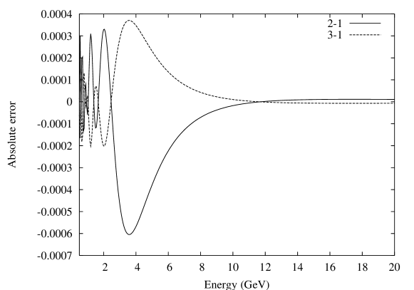
Figure 5: The effect of the astenospheric uncertainties to the muon neutrino appearance probability. Absolute differences of matter profiles 2 and 3 from the density profile 1 as a function of energy. (Parameters set as in Figure 3, with $\delta m_{32}^{2}>0$.)

4 Discussion

The PREM density profile is commonly used in Earth matter density neutrino oscillation studies. There has been discussion[28] about the accuracy of this approximate model. Therefore we also study the oscillation probability differences between the PREM and the realistic density profile.

We consider the $\nu_{e}\rightarrow\nu_{\mu}$ -oscillations. The absolute difference for the muon neutrino appearance probability between the two density profiles is shown in Figure 6. The difference of the appearance probability between the two density profiles is, around the first oscillation maximum, about a factor of 3 times larger than the error due to the astenospheric uncertainties. So, in obtaining the realistic density profile, the errors of neutrino oscillation simulations are a small step better, allthough they are not drastically improved.

Figure 6: The absolute difference of the muon neutrino appearance probabilities $P(\textrm{PREM})-P(\textrm{REAL})$. (Parameters set as in Figure 5.)

Random matter fluctuations of the density profile have been considered in Ref. [29]. It is estimated that with different realistical random matter fluctuations the average error of $P_{\mu e}$ for a distance $L\approx 2300$, average density $\rho=3$ g cm^-3 and energy $E_{\nu}=30$ GeV is $|\Delta P_{\mu e}|\sim 0.5\dots 1\cdot 10^{-5}$. In our case (with parameters as in Ref.[29]), the difference between the PREM and the realistic case is $|\Delta P_{\mu e}|=0.4\cdot 10^{-5}$ and $|\Delta P_{{\overline{\mu}}{\overline{e}}}|=0.6\cdot 10^{-5}$. Hence it seems that the error result from the random matter fluctuation model fits nicely in to our 2288 km baseline.

We will also like to point out that the calculated relative error between the neutrino factory beam muon event rates (from $\nu_{e}\rightarrow\nu_{\mu})$ using the PREM and realistic density profiles is below $\sim 2\%$ for beam energies around $1-10$ GeV and is considerably smaller for larger energies.

We conclude that we have made up a reference model for the CERN- Pyhäsalmi baseline that is accurate enough for all studies of long baseline neutrino oscillations. Although the results are quite similar to the PREM model, there is no excuse for using a less accurate model. However, for other baselines that have not been specifially modelled the PREM model may be a good approximation to start with.

The calculated event rates and parameter reaches of the CERN-Pyhäsalmi neutrino beam will be discussed in a future paper.

References

- [1] M. Apollonio et al., CERN-TH/2002-208
- [2] S. Malys, The WGS84 Reference Frame. National Imagery and mapping agency, Nov. 7, (1996).
- [3] M. Bursa, Earth, Moon and Planets, 69, 51 (1995)
- [4] D.J. Blundell, R. Freeman, St. Mueller, St. (ed) A continent revealed: the European Geotraverse 1992. Cambridge University Press, Cambridge (1992)
-
[5]
R. Artlitt, PhD Thesis, ETH, Zurich (1999)
S. Gregersen et al., Tectonophysics, 360, 61 (2002)
J. Plomerova et al., Tectonophysics, 360, 89 (2002) - [6] N. Cotte et al., Tectonophysics 360, 75 (2002)
-
[7]
S.-E. Hjelt and S. Daly et al., In D.G. Gee and H.J. Zeyen (ed) EUROPROBE 1996 - Lithospheric
dynamics: Origin and evolution of continents. Uppsala University (1996)
G. Bock (ed) et al., EOS Transactions AGU, 82, 50, 621, 628-629 (2001) - [8] E. Kozlovskaya et al. Geoph. J. Int., submitted (2003).
- [9] R. Carmichael (ed) Practical handbook of physical properties of rocks and minerals. CRC Press, Boca Raton, Florida (1989)
- [10] O.F. Gaul et al., Earth Plan. Sci. Lett., 182, 223 (2000).
- [11] C. Herzberg. Phase equilibra of common rocks in the crust and mantle. In: Ahrens, T. (ed) Rock physics and phase relations. A handbook of physical constants. AGU (1995).
- [12] E. Kozlovskaya and S.-E. Hjelt, Phys. and Chem. of the Earth (A),25, 2, 195 (2000)
-
[13]
S. Sobolev et al., Tectonophysics, 275, 143 (1997)
H. Sato et al., Pure Appl.Geoph., 153, 377 (1998)
C. Petit et al., Earth Plan. Sci. Lett.,197, 3-4, 133 (2002) - [14] M. Manghnani et al., J. Geoph. Res, 91, B9, 9333 (1996)
- [15] F. Deschamps et al., Phys. Earth Plan. Int., 124, 193 (2001)
-
[16]
G. Marquart and D. Lelgemann, Tectonophysics, 207,
25 (1992)
F. Cella et al., Tectonophysics, 287, 1-4, 117 (1998) - [17] P. Giese and H. Buness. Moho depth. In: D.J. Blundell, R. Freeman, St. Mueller (ed) A continent revealed: the European Geotraverse 1992. Cambridge University Press, Cambridge (1992)
- [18] A. Sommaruga, Marine and Petroleum Geology, 16, 111 (1999)
- [19] J. Ebbing, PhD Thesis, Fachbereich Geowissenschaften, Freie Universität Berlin (2002)
- [20] M.-A. Gutscher, Geophys. J. Int., 122, 617 (1995)
- [21] U. Achauer and F. Masson, Tectonophysics, 358, 17 (2002)
- [22] V. Babushka and J. Plomerova, Tectonophysics, 207,141 (1992).
- [23] L. Wolfenstein, Phys. Rev. D17, 2369 (1978)
- [24] K. Hagiwara et al., Phys. Rev. D66, 010001 (2002)
- [25] V. Barger et al., Phys. Rev. D62, 013004 (2000)
- [26] A. M. Dziewonski and D.L. Anderson, Phys. Earth Planet. Inter. 25, 297 (1981),
- [27] M. Apollonio et. al, Eur. Phys. J. C27, 331 (2003)
- [28] for example, see R. Geller and T. Hara, hep-ph/0111342 (2001)
- [29] B. Jacobsson et al., Phys. Lett. B532, 259 (2002)