Vector and axial-vector correlators in a nonlocal chiral quark model

Abstract

The behavior of nonperturbative parts of the isovector-vector and isovector and isosinglet axial-vector correlators at Euclidean momenta is studied in the framework of a covariant chiral quark model with nonlocal quark-quark interactions. The gauge covariance is ensured with the help of the $P$-exponents, with the corresponding modification of the quark-current interaction vertices taken into account. The low- and high-momentum behavior of the correlators is compared with the chiral perturbation theory and with the QCD operator product expansion, respectively. The $V-A$ combination of the correlators obtained in the model reproduces quantitatively the ALEPH data on hadronic $\tau$ decays, transformed into the Euclidean domain via dispersion relations. The predictions for the electromagnetic $\pi^{\pm}-\pi^{0}$ mass difference and for the pion electric polarizability are also in agreement with the experimental values. The topological susceptibility of the vacuum is evaluated as a function of the momentum, and its first moment is predicted to be $\chi^{\prime}(0)\approx(50\ \mathrm{MeV})^{2}$. In addition, the fulfillment of the Crewther theorem is demonstrated.

I Introduction

The vector ($V$) and axial-vector ($A$) current-current correlators are fundamental quantities of the strong-interaction physics, sensitive to small- and large-distance dynamics. They serve as an important testing ground for QCD as well as for effective models of strong interactions. In the limit of the exact isospin symmetry the $V$ and $A$ correlators in the momentum space (with $-q^{2}\equiv Q^{2}\geq 0$) are defined as

$$\Pi_{\mu\nu}^{V,ab}(q) = i\int d^{4}x~{}e^{iqx}\Pi_{\mu\nu}^{V,ab}(x)=\,\left(q_{\mu}q_{\nu}-g_{\mu\nu}q^{2}\right)\Pi_{T}^{V}(Q^{2})\delta^{ab},$$ (1)

$$\Pi_{\mu\nu}^{A,ab}(q) = i\int d^{4}x~{}e^{iqx}\Pi_{\mu\nu}^{A,ab}(x)=\,\left(q_{\mu}q_{\nu}-g_{\mu\nu}q^{2}\right)\Pi_{T}^{A}(Q^{2})\delta^{ab}+q_{\mu}q_{\nu}\Pi_{L}^{A}(Q^{2})\delta^{ab},$$ (2)

$$\qquad\Pi_{\mu\nu}^{J,ab}(x) = \langle 0\left|T\left\{J_{\mu}^{a}(x)J_{\nu}^{b}(0)^{\dagger}\right\}\right|0\rangle,$$

where the QCD currents are

$$J_{\mu}^{a}=\overline{q}\gamma_{\mu}T^{a}q,\qquad J_{\mu}^{5a}=\overline{q}\gamma_{\mu}\gamma_{5}T^{a}q,$$ (3)

and $T^{a}$ denote the generators of the $SU_{F}(2)$ flavor group, normalized to $\mathrm{tr}T^{a}T^{b}=\frac{1}{2}\delta^{ab}$. The momentum-space two-point correlation functions obey a (suitably subtracted) dispersion relation,

$$\Pi(Q^{2})=\frac{1}{\pi}\int_{0}^{\infty}\frac{ds}{s+Q^{2}}\mathrm{Im}\Pi(s),$$ (4)

where the imaginary parts of the correlators determine the spectral functions

$$v_{1}(s) = 4\pi\mathrm{Im}\Pi_{T}^{V}(s+i0),$$

$$a_{1}(s) = 4\pi\mathrm{Im}\Pi_{T}^{A}(s+i0).$$ (5)

Recently, the inclusive nonstrange $V$ and $A$ spectral functions have been determined separately and with high precision by the ALEPH ALEPH2 and OPAL OPAL collaborations from the hadronic $\tau$-lepton decays ($\tau\rightarrow\nu_{\tau}+$ hadrons) in the interval of invariant masses up to the $\tau$ mass, $0\leq s\leq m_{\tau}^{2}$.

The difference of the $V$ and $A$ correlation functions is very sensitive to the details of the spontaneous breaking of the chiral symmetry. In particular, the behavior of this combination is constrained by the chiral symmetry in the form of sum rules obtained through the use of the optical theorem WIII ; DMO ; DGMLY ; GasLeut85 . The experimental separation of the $V$ and $A$ spectral functions allows us to accurately test the chiral sum rules in the measured interval ALEPH2 ; OPAL . The coefficients of the Taylor expansion of the correlators at $Q^{2}=0$ are expressed in terms of the low-energy constants of the chiral perturbation theory($\chi$PT)GasLeut85 . On the other hand, the large-$s$ behavior of the correlators can be confronted with perturbative QCD thanks to the sufficiently large value of the $\tau$ mass. In the high-$s$ limit $\Pi^{V}(Q^{2})$ and $\Pi^{A}(Q^{2})$ are dominated by the free-field correlator, corrected by nonperturbative terms with inverse powers of $Q^{2}$. This follows from the fact that the correlators can be represented by an operator product expansion (OPE) series and thus are sensitive to the nonperturbative physics at smaller energy scales SVZ79 . Recently, the interest in the OPE expansion has been revived due to a possible appearance of unconventional quadratic power corrections, $\sim 1/Q^{2}$, found in CNZ , and also observed in lattice simulations Boucaud:2001st . The ALEPH and OPAL data have been intensely used in the literature in order to place limits on the leading coefficients of the $\chi$PT and OPE expansions (see, e.g, Davier:1998dz ; ioffe ; Geshkenbein:2002ri ; SHURYAK ; Klevansky:1997dk ; deRafael:2002tj ).

The aim of this work is to calculate the nonperturbative parts of the $V$ and $A$ current-current correlators in the kinematic region reaching up to moderately large Euclidean $Q^{2}$ and to extract experimentally observed characteristics. The calculations are carried out in the effective chiral model with nonlocal quark-quark interactions, which is made covariant by the inclusion of the $P$-exponents in the non-local interaction vertex. A specific prescription for the Wilson lines and their differentiation, described in Sec. III, follows exactly Ref. ADoLT00 . That way the model is made consistent with the gauge invariance and can be used to analyze the $V$ and $A$ correlators. The model is a nonlocal extension of the well-known Nambu-Jona Lasinio model. Moreover, its nonlocal structure may be motivated by fundamental QCD interactions induced by the instanton and gluon exchanges, which induce the spontaneous breaking of the chiral symmetry and generate dynamically a momentum-dependent quark mass. From the point of view of the standard OPE, the whole series of power corrections characterizes nonlocal properties of the QCD vacuum and may be described in terms of the nonlocal vacuum condensates MikhRad92 ; DEM97 . The use of a covariant nonlocal low-energy quark model based on the self-consistent approach to the dynamics of quarks has many attractive features, as it preserves the gauge invariance, is consistent with the low-energy theorems, as well as takes into account the large-distance dynamics controlled by the bound states. Similar models with nonlocal four-quark interaction have been considered earlier in, e.g., DP86 ; Tern91 ; IBGross92 ; Roberts:dr ; Birse95 ; DoLT98 ; Bron99 ; bled ; Golli ; Prasza and applied to describe various low-energy phenomena.

Nonlocal models have an important feature which makes them advantageous over the local models, such as the original Nambu–Jona-Lasinio model. At high virtualities the quark propagator and the vertex functions of the quark coupled to external fields reduce down to the free quark propagator and to local, point-like couplings. This property allows us to straightforwardly reproduce the leading terms of the operator product expansion. For instance, the second Weinberg sum rule is reproduced in the model Bron99 , which has not been the case of the local approaches. In addition, the intrinsic nonlocalities, inherent to the model, generate unconventional power and exponential corrections which have the same character as found in CNZ and in the instanton model (see e.g. SHURYAK ). Recently, the nonlocal effective model was successively applied to the description of the data from the CLEO collaboration on the pion transition form factor in the interval of the space-like momentum transfer squared up to 8 GeV² ADT99pigg ; AD02 . Importantly, in that study at zero photon virtualities the chiral anomaly result were reproduced, while at high photon virtualities the factorization of short and long distances occurs at a scale of the order of 1 GeV². This allowed for the extraction of the pion distribution amplitudes of leading and next-to-leading twists. There are several further advantages in using the nonlocal models compared to the local approaches. The non-local interactions regularize the theory in such a way that the anomalies are preserved Ripka93 ; Arrio . In other regularization methods in the local models mitia:rev ; Bijnens ; Goeke96 the preservation of the anomalies can only be achieved if the (finite) anomalous part of the action is left unregularized, and only the non-anomalous (infinite) part is regularized. Next, with non-local interactions the model is finite to all orders in the $1/N_{c}$ (loop) expansion. Finally, as shown in Golli , stable solitons exist in a chiral quark model with non-local interactions without the extra constraint that forces the chiral fields to lie on the chiral circle.

In the present paper we further test the nonlocal quark model by carrying out an analysis of the momentum dependence of the current-current correlators. A transformation of the spectral functions measured by the ALEPH collaboration into the Euclidean momentum space allows us for a precise an unambiguous comparison of the experimental data with the model calculations. The paper is organized as follows. In Sect. II, we briefly recall the results of the chiral perturbation theory and operator product expansion concerning the $V$ and $A$ correlators. In Sect. III and IV, we outline the gauged nonlocal quark model and introduce the quark-current vertices. Then, we derive the expressions for the nonperturbative parts of transverse $V$ and $A$ correlators (Sect. V) and, after fixing the model parameters in Sect. VI, confront the results with the available experimental data at large (Sect. VII) and low (Sect. VIII) Euclidean momenta. We explicitly demonstrate the transverse character of the $V$ and nonsinglet $A$ correlators in Sect. IX. In Sect. X the contribution of the $U_{A}(1)$ axial anomaly to the flavor-singlet longitudinal $A$ correlator is displayed and the topological susceptibility is calculated as a function of the momentum. Below, in all cases we use the strict chiral limit, with current quark mass equal to zero. Numerically current quark mass corrections to observables discussed in the paper do not exceed more than few percents.

II Chiral sum rules and the operator product expansion

Chiral sum rules are dispersion relations between the real and absorptive parts of a two-point correlation function that transforms symmetrically under $SU(2)_{L}\times SU(2)_{R}$ (for the case of non-strange currents). Through the use of the dispersion relations the sum rules are directly expressed in terms of the difference of the $V$ and $A$ spectral densities. Here is the list of sum rules, given in the strict chiral limit, which are investigated in this paper:

The first Weinberg sum rule (WSR I) WIII ,

$$\frac{1}{4\pi^{2}}\int_{0}^{s_{0}\rightarrow\infty}ds\left[v_{1}\left(s\right)-a_{1}\left(s\right)\right]=\left[-Q^{2}\Pi_{T}^{V-A}\left(Q^{2}\right)\right]_{Q^{2}\rightarrow 0}=f_{\pi}^{2},$$ (6)

the second Weinberg sum rule (WSR II) WIII ,

$$\frac{1}{4\pi^{2}}\int_{0}^{s_{0}\rightarrow\infty}dss\left[v_{1}\left(s\right)-a_{1}\left(s\right)\right]=Q^{2}\left[-Q^{2}\Pi_{T}^{V-A}\left(Q^{2}\right)\right]_{Q^{2}\rightarrow\infty}=0,$$ (7)

the Das-Mathur-Okubo (DMO) sum rule DMO ,

$$\frac{1}{4\pi^{2}}\int_{0}^{s_{0}\rightarrow\infty}ds\frac{1}{s}\left[v_{1}\left(s\right)-a_{1}\left(s\right)\right]=\left.\frac{\partial}{\partial Q^{2}}\left[Q^{2}\Pi_{T}^{V-A}\left(Q^{2}\right)\right]\right|_{Q^{2}\rightarrow 0}=f_{\pi}^{2}\frac{\left\langle r_{\pi}^{2}\right\rangle}{3}-F_{A},$$ (8)

and, finally, the Das-Guralnik-Mathur-Low-Yuong (DGMLY) sum rule DGMLY ,

$$-\frac{1}{4\pi^{2}}\int_{0}^{s_{0}\rightarrow\infty}dss\ln\frac{s}{\mu^{2}}\left[v_{1}\left(s\right)-a_{1}\left(s\right)\right]=\int_{0}^{\infty}dQ^{2}\left[-Q^{2}\Pi_{T}^{V-A}\left(Q^{2}\right)\right]=\frac{4\pi f_{\pi}^{2}}{3\alpha}\left[m_{\pi^{\pm}}^{2}-m_{\pi^{0}}^{2}\right],$$ (9)

where in the last equation $\alpha\approx 1/137$ is the fine structure constant. In the chiral limit of massless quarks the DGMLY sum rule is independent of the arbitrary normalization scale, $\mu^{2}$, thanks to WSR II. It was shown by Witten Witt83 that the positive electromagnetic mass shift of the charged pions is a consequence of the DGMLY sum rule combined with the positivity property of the $V-A$ correlator,

$$-Q^{2}\Pi_{T}^{V-A}\left(Q^{2}\right)\geqslant 0,\qquad\mathrm{for}\qquad 0\leqslant Q^{2}\leqslant\infty.$$ (10)

According to Witten, if the bare $u$ and $d$ quarks were massless and the mass shift were negative, the charged pions would become tachyons destabilizing the QCD vacuum.

Whereas WSR I and DMO are low-energy sum rules (in the sense that the right-hand sides involve correlators at low momenta), and are reproduced in most low-energy effective quark models, WSR II is a high-momentum sum rule. In local models it is not reproduced, as discussed shortly. The DMGLY sum rule collects contributions from the whole range of $Q^{2}$, both soft and hard.

The left hand sides of the sum rules (6)-(9) have been determined with the experimental data from ALEPH2 and OPAL , with $s_{0}$ taken as the upper limit of the interval of the invariant mass covered by the experiment. The right-hand sides of the sum rules are the theoretical predictions as $s_{0}\rightarrow\infty$. The DMO sum rule relates the derivative of $Q^{2}$ times the correlator to the square of the pion decay constant $f_{\pi}=\left(92.4\pm 0.3\right)\mathrm{MeV}$ PDG obtained from the decays $\pi^{-}\rightarrow\mu^{-}\overline{\nu}_{\mu}$ and $\pi^{-}\rightarrow\mu^{-}\overline{\nu}_{\mu}\gamma$, to the pion axial-vector form factor $F_{A}=0.0058\pm 0.0008$ for the radiative decays $\pi^{-}\rightarrow l^{-}\overline{\nu}_{l}\gamma$, and to the pion charge radius-squared $\left\langle r_{\pi}^{2}\right\rangle=\left(0.439\pm 0.008\right)$ fm² obtained from a one-parameter fit to the space-like data NA7 .

The listed chiral sum rules provide important restrictions on the correlators at low and high energies. The first Weinberg sum rule (6) fixes the normalization of correlators and holds in all variants of the Nambu–Jona-Lasinio models, local or nonlocal. In general, the coefficients of the Taylor expansion of the correlators at low Euclidean momenta are given by the low energy constants of the strong chiral Lagrangian. The second Weinberg sum rule (7) signals that the leading asymptotics of the high $Q^{2}$ power expansion of the $V-A$ correlator essentially starts from dimension $d=6$ term, and as such is valid in the nonlocal versions of the effective chiral quark models Bron99 . In local models WSR II involves on the right-hand side the large constituent quark mass times quark condensate, $M_{q}<\bar{q}q>$, thus is violated badly. In this regard the nonlocal models are highly rewarding.

More detailed short-distance, or large $Q^{2}$, properties of the correlators are represented by the QCD operator product expansion SVZ79 . For the $V-A$ and $V+A$ combinations the OPE provides the following leading-twist terms in the chiral limit:

$$\Pi_{T}^{V-A}(Q^{2}) = \sum_{d=6,8...}\frac{O_{V-A}^{d}}{Q^{d}}=\frac{O_{V-A}^{6}}{Q^{6}}+\mathcal{O}(\frac{1}{Q^{8}}),$$ (11)

$$\Pi_{T}^{V+A}(Q^{2}) = \sum_{d=0,2,4...}\frac{O_{V+A}^{d}}{Q^{d}}=$$

$$= -{\frac{1}{4\pi^{2}}}\left(1+\frac{\alpha_{s}}{\pi}\right)\ln\frac{Q^{2}}{\mu^{2}}-\frac{\alpha_{s}}{4\pi^{3}}\frac{\lambda^{2}}{Q^{2}}+\frac{1}{12}\frac{\left\langle\frac{\alpha_{s}}{\pi}\left(G_{\mu\nu}^{a}\right)^{2}\right\rangle}{Q^{4}}+\frac{O_{V+A}^{6}}{Q^{6}}+\mathcal{O}(\frac{1}{Q^{8}}),$$

where the vacuum matrix elements of dimension $d=6$ operators are

$$O_{V-A}^{6} = \pi\alpha_{s}\left[\left\langle\left(\overline{u}\gamma_{\mu}\lambda^{a}d\right)\left(\overline{d}\gamma_{\mu}\lambda^{a}u\right)\right\rangle-\left\langle\left(\overline{u}\gamma_{\mu}\gamma_{5}\lambda^{a}d\right)\left(\overline{d}\gamma_{\mu}\gamma_{5}\lambda^{a}u\right)\right\rangle\right],$$ (13)

$$O_{V+A}^{6} = -\pi\alpha_{s}\left[\left\langle\left(\overline{u}\gamma_{\mu}\gamma_{5}\lambda^{a}d\right)\left(\overline{d}\gamma_{\mu}\gamma_{5}\lambda^{a}u\right)\right\rangle+\left\langle\left(\overline{u}\gamma_{\mu}\lambda^{a}d\right)\left(\overline{d}\gamma_{\mu}\lambda^{a}u\right)\right\rangle+\frac{2}{9}\sum_{i=u,d}\sum_{j=u,d,s,...}\left\langle\left(\overline{q_{i}}\gamma_{\mu}\lambda^{a}q_{i}\right)\left(\overline{q_{j}}\gamma_{\mu}\lambda^{a}q_{j}\right)\right\rangle\right],$$

with $\lambda^{a}$ being the color $SU(3)$ matrices.

The ${V-A}$ correlator does not acquire any perturbative contribution in the limit of massless quarks, hence it is sensitive entirely to the chiral symmetry breaking parameters. Already at relatively small $Q^{2}$ the $d=6$ term dominates in the expansion of $\Pi_{V-A}$. On other hand, the sum of the correlators, $\Pi_{V+A}$, supplied with small power corrections, is close to the free-field result for distances up to 1 fm SHURYAK . In the expansion of $\Pi_{V+A}$ we also included $d=2$ term which violates the original OPE expansion of SVZ79 . Motivation for inclusion this term into consideration was given in CNZ . In (11) and (II) we do not explicitly show exponentially suppressed terms that may be induced by existence of instantons SVZ79 . The magnitudes of the vacuum matrix elements which appear in the OPE can not be fixed from the first principles and are fitted to various hadronic observables. Clearly, their determination is bound to carry experimental and theoretical uncertainties. Only a sign of the $d=6$ term in the $V-A$ correlator is fixed by the Witten inequality: $O_{V-A}^{6}\leqslant 0$.

Different models are used to estimate the vacuum expectation values. The standard approach in the calculation of the dimension $d=6$ matrix elements suggested and used in original work SVZ79 was to explore the factorization hypothesis, i.e. the saturation of the four-quark matrix elements with the intermediate vacuum state. Under this assumptions for the dimension $d=6$ matrix elements one gets

$$\left[O_{V-A}^{6}\right]^{\mathrm{factor}}=-32\pi\alpha_{s}\left\langle\overline{q}q\right\rangle^{2}/9,\qquad\left[O_{V+A}^{6}\right]^{\mathrm{factor}}=64\pi\alpha_{s}\left\langle\overline{q}q\right\rangle^{2}/81.$$ (14)

However, some authors conclude that probably the factorization hypothesis is violated by a factor of 2-3 Narison . Moreover, quite different result appears if one uses the instanton liquid model to calculate these matrix elements Shuryak:1982I ; Shuryak:82II .

In this work, for comparison with other model results, we use the following typical values of the condensates found via standard QCD sum rules without and with the inclusion of the $d=2$ term:

$$\frac{\alpha_{s}}{\pi}\lambda^{2}=0,\qquad\qquad\qquad\left\langle\frac{\alpha_{s}}{\pi}\left(G_{\mu\nu}^{a}\right)^{2}\right\rangle=0.012\mathrm{~{}GeV}^{4},\qquad\alpha_{s}\left\langle\overline{q}q\right\rangle^{2}=2.4\cdot 10^{-4}\mathrm{~{}GeV}^{6}\qquad\qquad[7,11],$$ (15)

$$\frac{\alpha_{s}}{\pi}\lambda^{2}=-0.12\mathrm{~{}GeV}^{2},\qquad\left\langle\frac{\alpha_{s}}{\pi}\left(G_{\mu\nu}^{a}\right)^{2}\right\rangle=0.022\mathrm{~{}GeV}^{4},\qquad\alpha_{s}\left\langle\overline{q}q\right\rangle^{2}=5.8\cdot 10^{-4}\mathrm{~{}GeV}^{6}\qquad\qquad[42].$$ (16)

The above values hold at a typical renormalization scale of about 1 GeV.

III Gauging nonlocal models

In local theories, the gauge principle of the minimum action uniquely determines the interaction of the matter fields with the gauge fields. However, in nonlocal theories such an interaction may be introduced in various ways, and its transverse part cannot be uniquely defined Mand62 . In order to obtain the nonlocal action in a gauge-invariant form with respect to external fields $V$ and $A$, we define the delocalized quark field, $Q$, with the help of the Schwinger gauge phase factor, a.k.a. the Wilson line or the link operator,

$$Q(x,y)=P\exp\left\{i\int_{x}^{y}dz_{\mu}\left[V_{\mu}^{a}(z)+A_{\mu}^{a}(z)\gamma_{5}\right]T^{a}\right\}q(y),\qquad\overline{Q}(x,y)=Q^{\dagger}(x,y)\gamma^{0}.$$ (17)

Here $V_{\mu}^{a}(z)$ and $A_{\mu}^{a}(z)$ are the external gauge vector and axial-vector fields, respectively, and $P$ is the operator of ordering along the integration path, with $y$ denoting the position of the quark and $x$ being an arbitrary reference point. The $P$ operator arranges the matrices in each term of the expansion of the exponent from the left to the right in the order determined by the point $z$ moving along the path from $x$ to $y$.

We start with the nonlocal chirally invariant action which describes the interaction of soft quark fields. The nonlocal four-quark interaction is depicted in Fig. 1. The soft gluon fields have been integrated out. The corresponding gauge-invariant action for quarks interacting through nonperturbative exchanges can be expressed in a form similar to the Nambu–Jona-Lasinio model ADoLT00

$$S = \int d^{4}x\ \overline{q}(x)\gamma^{\mu}\left[i\partial_{\mu}-V_{\mu}\left(x\right)-\gamma_{5}A_{\mu}\left(x\right)\right]q(x)+$$ (18)

$$+ \frac{1}{2}G\int d^{4}X\int\prod_{n=1}^{4}d^{4}x_{n}\ f(x_{n})\left[\overline{Q}(X-x_{1},X)\Gamma_{i}Q(X,X+x_{3})\overline{Q}(X-x_{2},X)\Gamma_{i}Q(X,X+x_{4})\right],$$

where in the simplest version of the model the spin-flavor structure of the interaction is given by matrix product

$$\left(\Gamma_{i}\otimes\Gamma_{i}\right)=\left(1\otimes 1+i\gamma_{5}\tau^{a}\otimes i\gamma_{5}\tau^{a}\right).$$ (19)

In Eq. (18) $\overline{q}=(\overline{u},\overline{d})$ denotes the quark flavor doublet field, $G$ is the four-quark coupling constant, and $\tau^{a}$ are the Pauli isospin matrices.

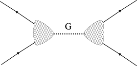
Figure 1: Diagrammatic representation of the effective nonlocal four-quark interaction of Eq. (18). The hatched blobs represent the nonlocal interactions, with the $\Gamma_{i}$ matrices present, and the dotted line indicates that the diagram can be cut across this line without crossing the quark lines going across the blobs.

The delocalization of the quark fields with the inclusion of the path-ordered Schwinger phase factors, Eq. (17), ensures the gauge invariance of the nonlocal action (18). However, the presence of these factors modifies the quark-current interaction, as shown graphically in Fig. (2). The modification of interaction, required by the gauge principle, poses a technical difficulty in dealing with nonlocal models, as many diagrams appear in the analysis of physical processes. The ambiguities in making the nonlocal 4-quark interaction gauge invariant are manifest in the path-dependence in the definition (17), as well as in the choice of the junction of the quark sources with the gauge strings. In general, the Noether currents consist of two components: the path-independent longitudinal part and the path-dependent transverse part. The dependence of the transverse component on the choice of the path is a feature of any method employed in constructing the Noether currents corresponding to a nonlocal action, and this freedom is immanent to the formulation of the model. We should recall here that the discussed ambiguities in the construction of the transverse parts of the Noether currents are by no means specific to chiral quark models. They also appear, e.g., in nuclear physics when one considers meson-exchange processes. To summarize, the choice of the path in Eq. (17) is a part of the model building.

In what follows, we use the formalism Mand62 ; Tern91 based on the path-independent definition of the derivative of the integral over a line for an arbitrary function $F_{\mu}(z)$:

$$\frac{\partial}{\partial y^{\mu}}\int_{x}^{y}dz^{\nu}\ F_{\nu}(z)=F_{\mu}(y),\qquad\delta^{(4)}\left(x-y\right)\int_{x}^{y}dz^{\nu}\ F_{\nu}(z)=0.$$ (20)

This choice effectively means that the differentiation involves moving the end-point of the line only, with the other part of the line kept fixed. As a result, the terms with nonminimal coupling, which are induced by the kinetic term of the action, are omitted.

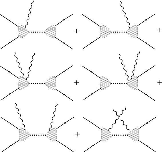
Figure 2: Diagrammatic representation of gauging of the effective nonlocal four-quark interaction (18), shown up to the second order in the expansion in external fields, represented by the wavy lines. Note that vertices involving one quark line and multiple gauge fields appear.

In general, external fields entering into Eq. (18) are arbitrary auxiliary fields; however, some of them can be associated with electromagnetic, weak, or strong interactions. In the case of the electromagnetic interactions, the gauge factor takes into account the effects of the radiation of the photon field when the two quarks are moving apart. This formalism was used in Tern91 ; IBGross92 ; Birse95 ; Bron99 ; DoLT98 to represent the nonlocal interaction in a gauge-invariant form. The incorporation of a gauge-invariant interaction with gauge fields is of principal importance if one desires to treat correctly the hadron characteristics probed by external currents, such as hadron electromagnetic and weak form factors, structure functions, distribution amplitudes, etc.

In Eq. (18) the functions $f(x_{n})$, normalized to $f(0)=1$, form the kernel of the four-quark interaction and characterize the space-dependence of the order parameter of the spontaneous chiral-symmetry breaking. Thus, the interaction is treated in the separable approximation. The choice of the nonlocal kernel in the form of (18) is motivated by the instanton-induced nonlocal quark-quark interaction DP86 , where the nonlocal function $f(x_{n})$ is related to the quark zero mode emerging in the instanton field DP86 ; DEM97 . To have the same flavor symmetry as in the original instanton-induced ’t Hooft determinant interaction one needs to add yet another piece of the form

$$G^{\prime}\left(\tau^{a}\otimes\tau^{a}+i\gamma_{5}\otimes i\gamma_{5}\right),$$ (21)

with the coupling $G^{\prime}=-G$. This term will be important in the discussion of the isosinglet axial currents in Sect. X. In the present work we do not consider an extended version of the model that explicitly includes vector and axial-vector degrees of freedom Birse95 (we take $G_{V}=0$, therefore $g_{A}=1$ and $M_{V}^{2},M_{A}^{2}\rightarrow\infty$).

In order to compute physical quantities we must first determine the full quark propagator and the full vertices for the vector and axial-vector currents. All calculations will be done in the leading order of the $1/N_{c}$ expansion, also referred to as the one-quark-loop level or the ladder approximation. In the nonlocal model the dressed quark propagator, $S(p)$, with the momentum-dependent quark scalar self-energy (mass), $M(p)$, is defined as

$$S^{-1}(p)=\widehat{p}-M(p).$$ (22)

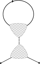
Figure 3: Diagrammatic representation of the quark scalar self-energy of Eq. (23).

Note that the considered model involves a constant quark wave-function renormalization function, $Z(p)=1$. The equation for the quark propagator in the ladder approximation, also known as the gap equation,

$$M(p)=4iGN_{f}N_{c}f^{2}(p)\int\frac{d^{4}k}{\left(2\pi\right)^{4}}f^{2}(k)\frac{M(k)}{k^{2}-M^{2}(k)}$$ (23)

has the formal solution Birse95 of the form

$$M(p)=M_{q}f^{2}(p),$$ (24)

with constant $M_{q}\equiv M(0)$ determined dynamically from Eq. (23). The quark self-energy is depicted in Fig. (3). Note that the functions $f(p)$ are treated non-dynamically, i.e. their dependence on $p$ is fixed, while $M(p)$ is dynamical. Furthermore, the integrals over the momentum are calculated by transforming the integration variables into the Euclidean space, ($k^{0}\rightarrow ik_{4},$ $k^{2}\rightarrow-k^{2}$).

IV Conserved vector and axial-vector currents

The Noether currents and the corresponding vertices are formally obtained as functional derivatives of the action (18) with respect to the external fields at the zero value of the fields. For our purpose, it is necessary to construct the quark-current vertices that involve one or two currents (contact terms). In the presence of the nonlocal interaction the conserved currents include both local and nonlocal terms. In order to expand the path-ordered exponent in the external fields, we use the technique described in Tern91 (see also Birse95 ; ADoLT00 ). Briefly, this method is as follows. First, the Fourier transform of the interaction kernel in Eq. (18) is obtained and expanded in the Taylor series in momemta. Next, the momentum powers are replaced by the derivatives acting on both the path-ordered exponent and the quark fields. Finally, the inverse Fourier transform is performed and summation is carried out again. The relations (20) and

$$\int d^{4}xF\left(x^{2}\right)e^{-ipx}\int_{y}^{\lambda x+a}dz^{\mu}\ e^{-iqz}=i\lambda\left(2p+q\lambda\right)^{\mu}\frac{F\left(p+\lambda q\right)-F\left(p\right)}{\left(p+\lambda q\right)^{2}-p^{2}}e^{-iqa}+F\left(p\right)\int_{y}^{a}dz^{\mu}\ e^{-iqz},$$ (25)

where $F(z^{2})$ is an arbitrary function, are frequently used in the procedure described above . The longitudinal projection of the above relation is

$$q^{\mu}\int d^{4}xF\left(x^{2}\right)e^{-ipx}\int_{y}^{\lambda x+a}dz^{\mu}\ e^{-iqz}=i\left[F\left(p+\lambda q\right)e^{-iqa}-F\left(p\right)e^{-iqy}\right].$$ (26)

The algebra needed to obtain the vertices with this method is straightforward but somewhat tedious, hence below we present only the final results.

The vector vertex following from the model (18) is (Fig. 4)

$$\Gamma_{\mu}^{a}(k,q,k^{\prime}=k+q)=T^{a}\left[\gamma_{\mu}-(k+k^{\prime})_{\mu}M^{(1)}(k,k^{\prime})\right],$$ (27)

where $M^{(1)}(k,k^{\prime})$ is the finite-difference derivative of the dynamical quark mass, $q$ is the momentum corresponding to the current, and $k$ $(k^{\prime})$ is the incoming (outgoing) momentum of the quark, $k^{\prime}=k+q$. The finite-difference derivative of an arbitrary function $F$ is defined as

$$F^{(1)}(k,k^{\prime})=\frac{F(k^{\prime})-F(k)}{k^{\prime 2}-k^{2}}.$$ (28)

Thus, with the gauging prescription given by (18) and (20), one gets the minimum-coupling vector vertex without extra transverse pieces. The form of the vertex is the same as the longitudinal vector vertex resulting from the Pagels-Stokar construction pagsto79 . The vertex satisfies the proper Ward-Takahashi identity:

$$q_{\mu}\Gamma_{\mu}^{a}(k,q,k^{\prime})=S_{F}^{-1}\left(k^{\prime}\right)T^{a}-T^{a}S_{F}^{-1}\left(k\right).$$ (29)

The vector vertex (27) is free of kinematic singularities and for this reason was advocated long ago in pagsto79 ; BallChiu . For the case of the momentum-independent mass, as in local models, the vertex (27) reduces to the usual local form, $\Gamma_{\mu}^{a}=T^{a}\gamma_{\mu}$.

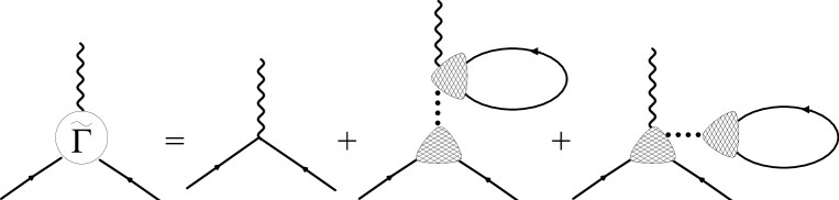
Figure 4: Diagrammatic representation of the bare quark-current vertices (27) and (IV).

The bare axial-vector vertex obtained from the action (18) by the differentiation with respect to the fields is given by the formula (cf. Fig. 4)

$$\widetilde{\Gamma}_{\mu}^{5a}(k,q,k^{\prime} = k+q)=T^{a}\left[\gamma_{\mu}-(k+k^{\prime})_{\mu}\frac{\left(\sqrt{M(k^{\prime})}-\sqrt{M(k)}\right)^{2}}{k^{\prime 2}-k^{2}}+\right.$$

$$\left.+\frac{q_{\mu}}{q^{2}}2\sqrt{M(k^{\prime})M(k)}\left[\frac{G}{M_{q}^{2}}J_{AP}(q^{2})-1\right]\right]\gamma_{5},$$

where we have introduced the notation

$$J_{AP}(q^{2}) = 4N_{c}N_{f}\int\frac{d^{4}l}{\left(2\pi\right)^{4}}\frac{M\left(l\right)}{D\left(l\right)}\sqrt{M\left(l+q\right)M\left(l\right)},$$ (31)

$$\qquad J_{AP}(q^{2} \rightarrow 0)=\frac{M_{q}^{2}}{G}-q^{2}J_{AP}^{\prime}(0)+O\left(Q^{4}\right),$$ (32)

with

$$J_{AP}^{\prime}(0)=\frac{N_{c}N_{f}}{32\pi^{2}}\int du\frac{uM\left(u\right)\left[4M^{\prime}\left(u\right)+2uM^{\prime\prime}\left(u\right)\right]-u\left(M^{\prime}\left(u\right)\right)^{2}}{D\left(u\right)},$$ (33)

where $u=k^{2}$ and (in the Euclidean space)

$$D\left(k\right)=k^{2}+M^{2}(k).$$ (34)

In Refs. HoldLew95 ; ADoLT00 it was demonstrated that in order to obtain the full vertex corresponding to the conserved axial-vector current it is necessary to add the term which contains the pion propagator. The presence of this term is associated with the well-known pion–axial vector mixing. The addition of the term with the pion propagator exactly cancels the third term in Eq. (IV), and the full conserved vertex acquires the form (cf. Figs. (5) and (6))

$$\Gamma_{\mu}^{5a}(k,q,k^{\prime}=k+q)=T^{a}\left[\gamma_{\mu}-q_{\mu}\frac{M(k^{\prime})+M(k)}{q^{2}}-(k+k^{\prime}-q\frac{k^{\prime 2}-k^{2}}{q^{2}})_{\mu}\frac{\left(\sqrt{M(k^{\prime})}-\sqrt{M(k)}\right)^{2}}{k^{\prime 2}-k^{2}}\right]\gamma_{5}.$$ (35)

It satisfies the axial Ward-Takahashi identity,

$$q_{\mu}\Gamma_{\mu}^{5a}(k,q,k^{\prime})=\gamma_{5}S_{F}^{-1}\left(k_{+}\right)T^{a}+T^{a}S_{F}^{-1}\left(k_{-}\right)\gamma_{5}.$$ (36)

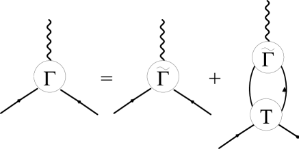
Figure 5: Diagrammatic representation of the full axial-vector vertex obtained from the bare axial vertex supplied with rescattering process of Fig. 6. In the present model there is no rescattering in the vector channel, and $\Gamma_{V}=\tilde{\Gamma}_{V}$.

The axial-vector vertex has a kinematic pole at $q^{2}=0$, a property that follows from the spontaneous breaking of the chiral symmetry in the limit of massless $u$ and $d$ quarks. Evidently, this pole corresponds to the massless Goldstone pion.

Figure 6: Diagrammatic representation of the quark-quark scattering matrix, $T$.

We also need the vertices that couple two currents to the quark (cf. Fig. 2). In this regard it is convenient to introduce the notation

$$G_{\mu}^{a}\left(k,q\right)=iT^{a}\left(2k+q\right)_{\mu}f^{(1)}(k,k+q),$$ (37)

and

$$G_{\mu\nu}^{ab}\left(k,q,q^{\prime},k^{\prime}\right) = -f\left(k^{\prime}\right)\left\{T^{a}T^{b}\left[g_{\mu\nu}f^{(1)}(k,k+q+q^{\prime})+\right.\right.$$

$$+ \left.\left.\left[2\left(k+q^{\prime}\right)+q\right]_{\mu}\left(2k+q^{\prime}\right)_{\nu}f^{(2)}\left(k,k+q^{\prime},k+q+q^{\prime}\right)\right]+\left[\left(q,a,\mu\right)\longleftrightarrow\left(q^{\prime},b,\nu\right)\right]\right\},$$

where the second finite-difference derivative is defined by

$$F^{(2)}\left(k,k^{\prime},k^{\prime\prime}\right)=\frac{F^{(1)}(k,k^{\prime\prime})-F^{(1)}(k,k^{\prime})}{k^{\prime\prime 2}-k^{\prime 2}}.$$ (39)

Further, we need to introduce

$$F_{\mu}^{(\pm)a}\left(k,q\right) = G_{\mu}^{a}\left(k,q\right)\pm G_{\mu}^{a}\left(k-q,q\right),$$ (40)

$$F_{\mu\nu}^{(\pm)ab}\left(k,q,q^{\prime},k^{\prime}\right) = G_{\mu\nu}^{ab}\left(k,q,q^{\prime},k^{\prime}\right)+G_{\mu\nu}^{ab}\left(k^{\prime}-q-q^{\prime},q,q^{\prime},k\right)$$ (41)

$$\pm G_{\mu}^{a}\left(k,q\right)G_{\nu}^{b}\left(k^{\prime}-q^{\prime},q^{\prime}\right)\pm G_{\mu}^{a}\left(k^{\prime}-q,q\right)G_{\nu}^{b}\left(k,q^{\prime}\right).$$

With the above definitions one gets for the $VV$ contact term

$$\Gamma_{\mu\nu}^{ab}(k,q,q^{\prime},k^{\prime}=k+q+q^{\prime}) = M_{q}F_{\mu\nu}^{(+)ab}\left(k,q,q^{\prime},k^{\prime}=k+q+q^{\prime}\right)$$

$$+ f(k)f(k^{\prime})G\int\frac{d^{4}l}{\left(2\pi\right)^{4}}Tr\left[S(l)F_{\mu\nu}^{(+)ab}\left(l,q,q^{\prime},l\right)\right].$$

For the $AA$ contact term one finds

$$\Gamma_{\mu\nu}^{5ab}(k,q,q^{\prime},k^{\prime}=k+q+q^{\prime})=\Gamma_{(1)\mu\nu}^{5ab}(k,q,q^{\prime},k^{\prime}=k+q+q^{\prime})+\Delta\Gamma_{\mu\nu}^{5ab}(k,q,q^{\prime},k^{\prime}=k+q+q^{\prime}),$$ (43)

where

$$\Gamma_{(1)\mu\nu}^{5ab}(k,q,q^{\prime},k^{\prime}=k+q+q^{\prime}) = M_{q}F_{\mu\nu}^{(-)ab}\left(k,q,q^{\prime},k^{\prime}=k+q+q^{\prime}\right)$$ (44)

$$+ f(k)f(k^{\prime})G\int\frac{d^{4}l}{\left(2\pi\right)^{4}}Tr\left[S(l)F_{\mu\nu}^{(-)ab}\left(l,q,q^{\prime},l\right)\right].$$ (45)

An additional contribution appears for the $AA$ iso-triplet contact term

$$\Delta\Gamma_{\mu\nu}^{5ab}(k,q,q^{\prime},k^{\prime} = k+q+q^{\prime})=-G\left[\tau^{c}G_{\nu}^{b}\left(k,q^{\prime}\right)-G_{\nu}^{b}\left(k-q^{\prime},q^{\prime}\right)\tau^{c}\right]$$

$$\times \left[\int\frac{d^{4}l}{\left(2\pi\right)^{4}}Tr\left[S(l)\tau^{c}F_{\mu}^{(-)a}\left(l,q\right)\right]\right]+\left[\left(q,\mu,a\right)\longleftrightarrow\left(q^{\prime},\nu,b\right)\right].$$

In the above expressions $Tr$ denotes the trace over flavor, color, and Dirac indices.

In the following we also need to introduce the polarization operator in the pseudoscalar channel (cf. Fig. 7),

$$J_{PP}(q^{2})\delta_{ab}=-\frac{i}{M_{q}^{2}}\int\frac{d^{4}k}{\left(2\pi\right)^{4}}M\left(k\right)M\left(k+q\right)Tr\left[S(k)\gamma_{5}\tau^{a}S\left(k+q\right)\gamma_{5}\tau^{b}\right]$$ (47)

and the correlator of the axial current vertex (IV) and the pion vertex (cf. Fig. 8)

$$\Gamma_{\pi}^{a}\left(k,k^{\prime}\right)=ig_{\pi}\gamma_{5}f(k)f(k^{\prime})\tau^{a},$$ (48)

defined by

$$J_{\pi A}\left(q^{2}\right)\delta_{ab}=\frac{q_{\mu}}{q^{2}}\int\frac{d^{4}k}{\left(2\pi\right)^{4}}Tr\left[S(k)\widetilde{\Gamma}_{\mu}^{5a}(k,q,k+q)S\left(k+q\right)\Gamma_{\pi}^{a}\left(k+q,k\right)\right].$$ (49)

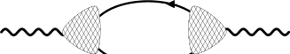
Figure 7: The polarization operator of Eq. (47)

Through the use of the gap equation (23) and the expression for the pion decay constant, $f_{\pi}$, given by DP86 ; Birse95

$$f_{\pi}^{2}=\frac{N_{c}}{4\pi^{2}}\int\limits_{0}^{\infty}du\ u\frac{M(u)^{2}-uM(u)M^{\prime}(u)+u^{2}M^{\prime}(u)^{2}}{D^{2}\left(u\right)},$$ (50)

these correlators have the following expansion at zero momentum:

$$J_{PP}(q^{2})=\frac{1}{G}+\frac{f_{\pi}^{2}}{M_{q}^{2}}q^{2}+O\left(q^{4}\right),\qquad J_{\pi A}\left(q^{2}\right)=f_{\pi}^{2}+O\left(q^{2}\right).$$ (51)

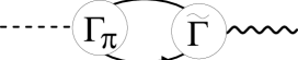
Figure 8: The correlator of the bare axial current vertex (IV) and the pion vertex (48).

In (50) we have used the notation $u=k^{2}$ and $M^{\prime}(u)=dM(u)/du$. In Eq. (48) the quark-pion coupling, $g_{\pi}^{2}=\left[J_{PP}^{\prime}(0)\right]^{-1}$, and the pion decay constant, $f_{\pi}$, are connected by the Goldberger-Treiman relation,

$$g_{\pi}=\frac{M_{q}}{f_{\pi}},$$ (52)

which is verified to be valid in the nonlocal model Birse95 , as required by the chiral symmetry.

V Current-current correlators (transverse parts)

Our goal is to obtain the nonperturbative parts of the current-current correlators from the effective model and to compare them with the existing $\tau$ decay data. The current-current correlators may be represented as a sum of two terms, dispersive (Fig. 9) and contact (Fig. 10), namely

$$-Q^{2}\Pi_{\mu\nu}^{J}\left(Q^{2}\right) = K_{\mu\nu}^{J}\left(Q^{2}\right)+S_{\mu\nu}^{J}\left(Q^{2}\right),$$ (53)

$$K_{\mu\nu}^{V}\left(Q^{2}\right) = \int\frac{d^{4}k}{\left(2\pi\right)^{4}}Tr\left[\Gamma_{\mu}^{V}\left(k,Q,k+Q\right)S\left(k+Q\right)\Gamma_{\nu}^{V}\left(k+Q,-Q,k\right)S\left(k\right)\right],$$ (54)

$$K_{\mu\nu}^{A}\left(Q^{2}\right) = \int\frac{d^{4}k}{\left(2\pi\right)^{4}}Tr\left[\Gamma_{\mu}^{A}\left(k,Q,k+Q\right)S\left(k+Q\right)\widetilde{\Gamma}_{\nu}^{A}\left(k+Q,-Q,k\right)S\left(k\right)\right],$$ (55)

$$S_{\mu\nu}^{J}\left(Q^{2}\right) = 2M_{q}\int\frac{d^{4}k}{\left(2\pi\right)^{4}}Tr\left[S\left(k\right)\Gamma_{\mu\nu}^{J}\left(k,Q,-Q,k+Q\right)\right].$$ (56)

The vertices $\Gamma_{\mu}^{J}\left(k,q,k^{\prime}\right)$ are given in Eqs. (27,35), $\Gamma_{\mu\nu}^{J}\left(k,q,q^{\prime},k^{\prime}\right)$ in Eq. (IV,43), and $\widetilde{\Gamma}_{\mu\nu}^{A}\left(k,q,q^{\prime},k^{\prime}\right)$ in Eq. (IV). The difference in the definitions of $K_{\mu\nu}\left(Q^{2}\right)$ in (54) and (55) results from the necessity of taking into account the rescattering diagrams in the axial channel of the pseudoscalar ($\pi$ or $\eta^{\prime}$) mesons (Fig. 9). The correlators (53) are defined in such a way that the perturbative contributions are subtracted,

$$\Pi_{np}\left(Q^{2}\right)=\Pi_{tot}\left(Q^{2}\right)-\Pi_{pert}\left(Q^{2}\right).$$ (57)

The perturbative part is obtained from the non-perturbative part by simply setting the dynamical quark mass $M(k)$ to zero. We extract the longitudinal and transverse parts of the correlators through the use of the projectors

$$P_{\mu\nu}^{L}=\frac{q^{\mu}q^{\nu}}{q^{2}},\qquad P_{\mu\nu}^{T}=\frac{1}{3}\left(g_{\mu\nu}-\frac{q^{\mu}q^{\nu}}{q^{2}}\right).$$ (58)

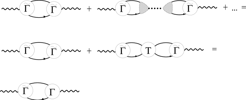
Figure 9: The resummation of the quark rescattering in the current-current correlator in the axial-vector channel.

We first consider the transverse part of the $V$ correlator, with the result

$$K_{T}^{V}\left(Q^{2}\right) = 2N_{c}\int\frac{d^{4}k}{\left(2\pi\right)^{4}}\frac{1}{D_{+}D_{-}}\left\{M_{+}M_{-}+\left[k_{+}k_{-}-\frac{2}{3}k_{\perp}^{2}\right]_{np}\right.$$

$$+ \left.\frac{4}{3}k_{\perp}^{2}\left[\left(\frac{M_{+}-M_{-}}{k_{+}^{2}-k_{-}^{2}}\right)^{2}\left(k_{+}k_{-}-M_{+}M_{-}\right)-\frac{M_{+}^{2}-M_{-}^{2}}{k_{+}^{2}-k_{-}^{2}}\right]\right\},$$

$$S_{T}^{V}\left(Q^{2}\right) = 4N_{c}\int\frac{d^{4}k}{\left(2\pi\right)^{4}}\frac{M\left(k\right)}{D\left(k\right)}\left\{M^{\prime}\left(k\right)+\frac{4}{3}\frac{k_{\perp}^{2}}{k^{2}-\left(k+Q\right)^{2}}\left(M^{\prime}\left(k\right)-\frac{M\left(k+Q\right)-M\left(k\right)}{\left(k+Q\right)^{2}-k^{2}}\right)\right\},$$ (60)

where the notations $k_{\perp}^{\mu}=k^{\mu}-Q^{\mu}(kQ)/Q^{2}$, $k_{\pm}=k\pm Q/2$,

$$M_{\pm}=M(k_{\pm}),\ \ \ \ \ D_{\pm}=D(k_{\pm})$$ (61)

have been introduced. The subtraction of the perturbative part amounts to the replacement

$$\frac{1}{D_{+}D_{-}}\left[k_{+}k_{-}-\frac{2}{3}k_{\perp}^{2}\right]_{np}\Longrightarrow\left[k_{+}k_{-}-\frac{2}{3}k_{\perp}^{2}\right]\left[\frac{1}{D_{+}D_{-}}-\frac{1}{k_{+}^{2}k_{-}^{2}}\right].$$ (62)

Further, we take the nonsinglet transverse projection of the $A$ correlator and obtain

$$K_{T}^{A}\left(Q^{2}\right) = 2N_{c}\int\frac{d^{4}k}{\left(2\pi\right)^{4}}\frac{1}{D_{+}D_{-}}\left\{-M_{+}M_{-}+\left[k_{+}k_{-}-\frac{2}{3}k_{\perp}^{2}\right]_{np}+\right.$$

$$+ \left.\frac{4}{3}k_{\perp}^{2}\left[\frac{\left(\sqrt{M_{+}}-\sqrt{M_{-}}\right)^{4}}{\left(k_{+}^{2}-k_{-}^{2}\right)^{2}}\left(k_{+}k_{-}+M_{+}M_{-}\right)-\frac{\left(M_{+}-M_{-}\right)\left(\sqrt{M_{+}}-\sqrt{M_{-}}\right)^{2}}{k_{+}^{2}-k_{-}^{2}}\right]\right\},$$

$$S_{T}^{A}\left(Q^{2}\right) = S_{T}^{V}\left(Q^{2}\right)-4N_{c}\int\frac{d^{4}k}{\left(2\pi\right)^{4}}\frac{M\left(k\right)}{D\left(k\right)}\frac{8}{3}k_{\perp}^{2}\frac{\left(\sqrt{M\left(k+Q\right)}-\sqrt{M\left(k\right)}\right)^{2}}{\left[\left(k+Q\right)^{2}-k^{2}\right]^{2}}.$$ (64)

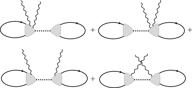
Figure 10: The contact terms in the current-current correlators.

Let us consider the difference of the $V$ and $A$ correlators, where a number of cancellations takes place and the final result is quite simple,

$$-Q^{2}\Pi^{V-A}\left(Q^{2}\right) = 4N_{c}\int\frac{d^{4}k}{\left(2\pi\right)^{4}}\frac{1}{D\left(k_{+}^{2}\right)D\left(k_{-}^{2}\right)}\left\{M_{+}M_{-}+\frac{4}{3}k_{\perp}^{2}\left[-\sqrt{M_{+}M_{-}}\frac{M_{+}-M_{-}}{k_{+}^{2}-k_{-}^{2}}\right.\right.$$

$$+ \left.\left.\frac{\left(\sqrt{M_{+}}-\sqrt{M_{-}}\right)^{2}}{\left(k_{+}^{2}-k_{-}^{2}\right)^{2}}\left(\sqrt{M_{+}}k_{+}+\sqrt{M_{-}}k_{-}\right)^{2}\right]\right\}.$$

One may explicitly verify that the integrand of the above expression is indeed positive-definite, irrespectively of the choice of the mass function $M(p)$. Thus the Witten inequality (10) is indeed fulfilled.

At $Q^{2}=0$ one gets the results consistent with the first Weinberg sum rule,

$$-Q^{2}\Pi^{V,T}\left(Q^{2}=0\right)=0,\qquad-Q^{2}\Pi^{A,T}\left(Q^{2}=0\right)=-f_{\pi}^{2},\qquad-Q^{2}\Pi^{V-A,T}\left(Q^{2}=0\right)=f_{\pi}^{2},$$ (66)

where the explicit definition of the pion decay constant (50) is used. This serves as a useful algebraic check.

VI Model parameters

The parameters of the model are fixed in a way typical for effective low-energy quark models. We demand that the pion decay constant $f_{\pi}$, (50), and the quark condensate (for a single flavor), $<\bar{q}q>$, given by

$$\langle\bar{q}q\rangle=-\frac{N_{c}}{4\pi^{2}}\int du\ u\frac{M(u)}{D\left(u\right)},$$ (67)

acquire their physical values. For simplicity, we take profile for the dynamical quark mass in a Gaussian form

$$M(u)=M_{q}\exp\left(-2u/\Lambda^{2}\right).$$ (68)

With the model parameters

$$M_{q}=0.3~{}\mathrm{GeV,}\qquad\Lambda=1.085~{}\mathrm{GeV,}$$ (69)

one obtains

$$f_{\pi}=93~{}\mathrm{MeV,}\qquad\langle\bar{q}q\rangle=-\left(224~{}\mathrm{MeV}\right)^{3},$$ (70)

where the quark condensate is supposed to be normalized at the scale of a few hundred MeV.

VII Large-$Q^{2}$ expansion

At large $Q^{2}$ one finds the following asymptotic expansion for the difference and sum of the correlation functions in the inverse powers of $Q^{2}$ (we do not display here the exponentially-suppressed terms coming from powers of the dynamical quark-mass form factor):

$$\left.-Q^{2}\Pi^{V-A}\left(Q^{2}\right)\right|_{Q^{2}\rightarrow\infty} = \frac{2}{Q^{4}}\frac{N_{c}}{4\pi^{2}}\int du\frac{u^{2}M^{2}\left(u\right)}{D\left(u\right)}+\mathcal{O}\left(\frac{1}{Q^{6}}\right),$$ (71)

$$-Q^{2}\Pi_{T}^{V+A}\left(Q^{2}\rightarrow\infty\right) = 2\frac{N_{c}}{4\pi^{2}}\int du\frac{u}{D\left(u\right)}\left[M\left(u\right)M^{\prime}\left(u\right)\left(1-\frac{u}{Q^{2}}-\frac{2}{3}\frac{u^{2}}{Q^{4}}\right)-\frac{7}{6}\frac{uM^{2}\left(u\right)}{Q^{4}}\right]+\mathcal{O}\left(\frac{1}{Q^{6}}\right).$$ (72)

The effective model considered here is designed to describe low energy physics. At high energies it is certainly not expected to reproduce all the details of the asymptotic standard operator product expansion of QCD. On other hand, it is possible that the OPE works well only at very short distances while the effective model is applicable at large and intermediate distances. With this hope in mind we proceed to analyzing the large-$Q^{2}$ expansions of the correlators, comparing them numerically to the OPE results, and trying to match the two approaches. It is important to note that the power corrections in the expansions (71) and (72) have the same inverse powers of $Q^{2}$ as the OPE.

We may now compare the expansion of the model correlators to the OPE , Eqs. (11,II). In Eq. (71) the formally leading $d=4$ term absent in the chiral limit in accordance with the second Weinberg sum rule and the OPE QCD. The second term in Eq. (71) (and the last term in Eq. (72)) is proportional to the derivative of the gluon condensate, and via equations of motion it reduces to the four-quark condensate term appearing in the OPE, Eqs. (11,II). Let us compare the numerical estimates for the local $d=6$ terms obtained from the QCD sum rules and from the nonlocal chiral quark model, labeled as N$\chi$QM:

$$\left[O_{6}^{V-A}\right]^{\mathrm{QCDsr}} \approx -(1\div 2)\cdot 10^{-3}\mathrm{~{}GeV}^{6},\qquad$$ (73)

$$\left[O_{6}^{V-A}\right]^{\mathrm{OPE\tau}} = -(3.4\pm 1.1)\cdot 10^{-3}\mathrm{~{}GeV}^{6},\qquad$$

$$\left[O_{6}^{V-A}\right]^{N\chi QM} = -1.1\cdot 10^{-3}\mathrm{~{}GeV}^{6}.$$

The first estimate is found on the basis of low energy theorems and QCD sum rules SVZ79 , while the second estimate is made with the help of the $\tau$-decay data ioffe . The result of the present model is closer to the standard estimate obtained from the low-energy phenomenology. Similar features of the short-distance behavior of the correlators were found in the instanton model SHURYAK .

In the $V+A$ correlator (72) the short-distance expansion contains, in addition to the contributions coming from the local operators, the unconventional terms originating from the nonlocal operators of dimension $d=2,4$ and $6$ (the first terms in Eq. (72)). This kind of unconventional terms has recently attracted attention due to the revision of the standard OPE CNZ , as well as the lattice findings, where the unconventional power corrections in the vector correlators were reported Boucaud:2001st . The appearance of this correction is usually related to the existence of the lowest $d=2$ condensate $\left\langle\left(A_{\mu}^{a}\right)^{2}\right\rangle$, which is due to an apparent gauge non-invariance, absent in the standard OPE. However, in a series of papers (Stodolsky:2002st ; Dudal:2003vv , and references therein) it was argued that it is possible to define the nonlocal operator with the lowest dimension in a gauge-invariant way. This situation is very similar to the famous spin-crisis problem (cf. Dorokhov:ym ). Analogously, in that case there is no twist-two gluonic operator that may contribute to the singlet axial current matrix element, yet, it is possible to construct the matrix element from nonlocal operators Jaffe:1989jz . We thus see that our effective nonlocal model shares these unusual effects generated by the internal nonlocalities of the quark interaction. Furthermore, the lowest-dimension power corrections are naturally present in the approaches similar to the analytic perturbative theory DVSol . In that case in order to compensate the effects of the ghost pole in the strong coupling constant, the $d=2$ power term is added. As discussed in Ref. Narison:2001ix , the justification of the appearance of the unconventional power corrections at the same time means that the standard OPE is valid only at very large momenta.

We also wish to comment that in the model expansion of the $V+A$ correlator there are no explicit terms with the gluon condensate of dimension $d=4$. The appearance of this term in the nonlocal chiral quark model would corresponded to the local matrix element

$$\frac{N_{c}}{4\pi^{2}}\int du\frac{uM^{2}\left(u\right)}{D\left(u\right)},$$

that is related to the gluon condensate through the gap equation (23) DP85 . However, the coefficient of this term is equal to zero. This is due to the simple form of the quark propagator (22), which does not allow gluonic correlations between different quark lines. The similar situation occurs in the QCD sum rules calculations (in the fixed point gauge), where nonzero contribution comes from the diagram with quark lines correlated by soft gluon exchange. These (numerically small) correlation terms may be reconstructed in the effective model by introducing the gluonic field in the effective action (18) by gauging kinetic and interaction terms (see also cf. Bijnens ). From other hand the $d=4$ term appears in (72) as a nonlocal matrix element.

We end the discussion of the short-range behavior of the correlators by giving the numerical estimates of the additional terms appearing in Eq. (72):

$$\left[O_{2}^{V+A}\right]_{\mathrm{nonloc}}^{N\chi QM} = -\frac{N_{c}}{2\pi^{2}}\int du\frac{u}{D\left(u\right)}M\left(u\right)M^{\prime}\left(u\right)=5.0\cdot 10^{-3}\mathrm{~{}GeV}^{2},$$ (74)

$$\left[O_{4}^{V+A}\right]_{\mathrm{nonloc}}^{N\chi QM} = \frac{N_{c}}{2\pi^{2}}\int du\frac{u^{2}}{D\left(u\right)}M\left(u\right)M^{\prime}\left(u\right)=-1.8\cdot 10^{-3}\mathrm{~{}GeV}^{4},$$

$$\left[O_{6}^{V+A}\right]_{\mathrm{nonloc}}^{N\chi QM} = \frac{4}{3}\frac{N_{c}}{4\pi^{2}}\int du\frac{u^{3}}{D\left(u\right)}M\left(u\right)M^{\prime}\left(u\right)=-7.6\cdot 10^{-4}\mathrm{~{}GeV}^{6}.$$

The sum of these terms, taken in the interval of momenta $Q^{2}\sim\left(1\div 2\right)$ GeV² where the model large-$Q^{2}$ expansion is expected to be valid, agrees reasonably well with the coefficient of the leading power correction in Eq. (II)

$$\left[O_{2}^{V+A}\right]^{\mathrm{QCDsr}}=3.0\cdot 10^{-3}\mathrm{~{}GeV}^{2},$$ (75)

where we have taken the estimate $\left(\alpha_{s}/\pi\right)\lambda^{2}=-0.12\mathrm{~{}GeV}^{2}$ from Ref. Narison:2001ix .

Through the use of the factorization hypothesis (14) it is predicted that the chirality flip matrix element $O_{6}^{V-A}$ is strongly enhanced in absolute value over the chirality nonflip one $O_{6}^{V+A}$

$$\left[O_{6}^{V-A}/O_{6}^{V+A}\right]^{\mathrm{factor}}=-4.5.$$ (76)

In the nonlocal chiral quark model the chirality flip matrix element $O_{6}^{V-A}$ is given by the local matrix element, but the chirality nonflip one $O_{6}^{V+A}$ is a mixture of the local and nonlocal matrix elements which transform to each other by integration by parts. We find that their ratio

$$\left[O_{6}^{V-A}/O_{6}^{V+A}\right]^{N\chi QM}\approx-3.2$$ (77)

has the same tendency as predicted in (76). It happens due to partial compensation of contributions of the local and nonlocal matrix elements into $O_{6}^{V+A}.$

VIII Low-energy observables and the ALEPH data

Let us now consider the low-energy region where the effective model (18) should be fully predictive. From (V) and the DGMLY sum rule (9) we estimate the electromagnetic pion mass difference to be

$$\left[m_{\pi^{\pm}}-m_{\pi^{0}}\right]_{N\chi QM}=4.2\mathrm{~{}MeV},$$ (78)

which is in remarkable agreement with the experimental value (after subtracting the $m_{d}-m_{u}$ effect) GasLeut85

$$\left[m_{\pi^{\pm}}-m_{\pi^{0}}\right]_{\mathrm{exp}}=4.43\pm 0.03\mathrm{~{}MeV}.$$ (79)

It is interesting to estimate the electric polarizability of the charged pions, Petrun ; DorVoHuKle97 . With the help of the DMO sum rule , as done by Gerasimov in Geras79 , we find

$$\alpha^{E}_{\pi^{\pm}}=\frac{\alpha}{m_{\pi}}\left[\frac{\left\langle r_{\pi}^{2}\right\rangle}{3}-\frac{I_{DMO}}{f_{\pi}^{2}}\right],$$ (80)

where $I_{DMO}$ is the left-hand side of the DMO sum rule (8)

$$I_{DMO}\left(s_{0}\right)=\frac{1}{4\pi^{2}}\int_{0}^{s_{0}}\frac{ds}{s}\left[v_{1}\left(s\right)-a_{1}\left(s\right)\right].$$ (81)

Equation (80) can be interpreted as a sum of the center-of-mass recoil contribution and the intrinsic pion polarizability. In Geras79 it was demonstrated that in model calculations there occurs a delicate cancellation between the two contributions of Eq. (80). This requires the calculation of both terms consistently at the same level of approximations.

With the experimental value for the pion mean squared radius NA7 and the value of the $I_{DMO}$ integral estimated from the ALEPH and OPAL data OPAL

$$\left[I_{DMO}\left(m_{\tau}^{2}\right)\right]_{\mathrm{exp}}=\left(26.3\pm 1.8\right)\cdot 10^{-3}$$ (82)

one gets from Eq. (80) the result OPAL

$$\left[\alpha^{E}_{\pi^{\pm}}\right]_{\mathrm{exp}}=\left(2.71\pm 0.88\right)\cdot 10^{-4}\mathrm{~{}fm}^{3}.$$ (83)

From Eq. (8) also follows the relation obtained by Terentyev Teren72 , which relates the pion polarizability and the pion axial-vector form factor,

$$\alpha^{E}_{\pi^{\pm}}=\frac{\alpha F_{A}}{m_{\pi}f_{\pi}^{2}}.$$ (84)

The last relation, used with the known values for $F_{A}$, yields

$$\alpha^{E}_{\pi^{\pm}}=\left(2.69\pm 0.37\right)\cdot 10^{-4}\mathrm{~{}fm}^{3},$$ (85)

which is very close to (83).

Let us estimate the electric polarizability of the charged pions within the nonlocal chiral quark model. By calculating the derivative of $\Pi^{V-A}\left(Q^{2}\right)$ at zero momentum we estimate the left hand side of the DMO sum rule as

$$\left[I_{DMO}\left(s_{0}\rightarrow\infty\right)\right]_{N\chi QM}=18.2\cdot 10^{-3}.$$ (86)

The value of the pion charge radius squared,

$$\left[\left\langle r_{\pi}^{2}\right\rangle\right]_{N\chi QM}=0.33\quad\mathrm{fm}^{2},$$ (87)

obtained in our model from the derivative of the charged pion form factor, is close to its limit of the local chiral model, found by Gerasimov long ago Geras79 ,

$$\left[\left\langle r_{\pi}^{2}\right\rangle\right]_{\chi PT}=\frac{N_{c}}{4\pi^{2}f_{\pi}^{2}}=0.34\quad\mathrm{fm}^{2}.$$ (88)

The model predictions for $\left\langle r_{\pi}^{2}\right\rangle$ and $I_{DMO}$ are somewhat smaller than the experimental values given above. The reason for this discrepancy may be attributed to vector meson degrees of freedom, neglected in our treatment, and to pion loops absent in the large-$N_{c}$ limit. However, these unconsidered contributions are essentially canceled in the combination (4) defining the electric pion polarizability (see, e.g. Klevansky:1997dk for discussions). From (80) we find with values given in Eqs. (86) and (87) the value

$$\left[\alpha^{E}_{\pi^{\pm}}\right]_{N\chi QM}=2.9\cdot 10^{-4}\mathrm{fm}^{3},$$ (89)

which is close to experimental number (83) and also to the prediction of the chiral perturbation theory at the one-loop level burgi ,

$$\left[\alpha^{E}_{\pi^{\pm}}\right]_{\chi\mathrm{PT}}=2.7\cdot 10^{-4}\mathrm{fm}^{3}.$$ (90)

Let us note also that (89) is a factor of 2 smaller from the estimates obtained in a local chiral quark model KlevPolariz99 , $\alpha^{E}_{\pi^{\pm}}=5.8\cdot 10^{-4}\mathrm{~{}fm}^{3}$. We thus see that the model prediction for the pion polarizability, Eq. (89), is in a very reasonable agreement with the experimental data.

Figure 11: Inclusive vector minus axial vector spectral function, $v_{1}-a_{1}$, measured by the ALEPH collaboration ALEPH2 .

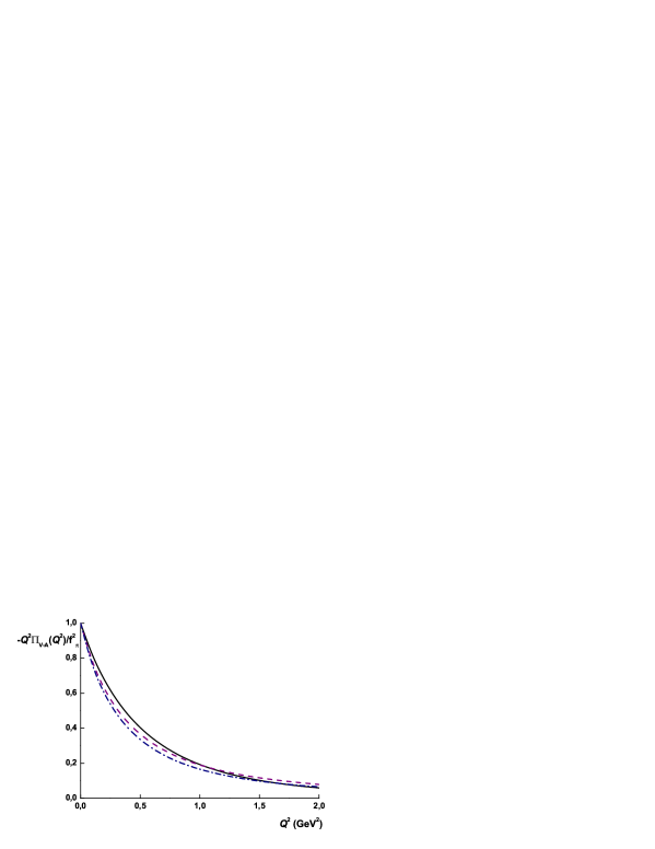
Figure 12: Euclidean-momentum correlation function, $-Q^{2}\Pi_{V-A}(Q^{2})/f^{2}_{\pi}$, constructed in the present model (solid line), in the model of Ref. deRafael:2002tj (dashed line), and reconstructed via Eq. (91) from the ALEPH experimental spectral function of Fig. 11 (dash-dotted line).

Next, we compare the model correlators with the ALEPH data, presented in Fig. 11. The ALEPH and OPAL data integrated up to the $\tau$ mass satisfy all chiral sum rules within the experimental uncertainty, but the central values differ significantly from the chiral model predictions. Following Ref. SHURYAK we use $s_{0}=2.5$ GeV² as an upper integration limit, the value at which all chiral sum rules are satisfied assuming that $v_{1}(s)-a_{1}(s)=0$ above $s_{0}$. Finally, a kinematic pole at $q^{2}=0$ is added to the axial-vector spectral function. The resulting unsubtracted dispersion relation between the measured spectral densities and the correlation functions becomes

$$\Pi_{V}^{T}\left(Q^{2}\right)-\Pi_{A}^{T}\left(Q^{2}\right)=\frac{1}{4\pi^{2}}\int_{0}^{s_{0}}ds\frac{v_{1}(s)-a_{1}(s)}{s+Q^{2}}-\frac{f_{\pi}^{2}}{Q^{2}},$$ (91)

where $f_{\pi}^{2}$ is given by the WSR I,

$$f_{\pi}^{2}=\frac{1}{4\pi^{2}}\int_{0}^{s_{0}}ds\left[v_{1}(s)-a_{1}(s)\right].$$ (92)

Having transformed the data into the Euclidean space, we may now proceed with the comparison to the model, which obviously applies to the Euclidean domain only. Admittedly, in the Euclidean presentation of the data the detailed resonance structure corresponding to the $\rho$ and $a_{1}$ mesons seen in the Minkowski region is smoothed out, hence the verification of model results is not as stringent as would be directly in the Minkowski space. In Fig. 12 we show the normalized curves corresponding to the experimental data and the model prediction. We also show the prediction of the model of Ref. deRafael:2002tj (minimal hadronic approximation, MHA DeRaf98 ; Anri01 )

$$\left[\Pi_{V-A}^{T}\left(Q^{2}\right)\right]_{MHA}=\frac{f_{\rho}^{2}M_{\rho}^{2}}{Q^{2}+M_{\rho}^{2}}-\frac{f_{a}^{2}M_{a}^{2}}{Q^{2}+M_{a}^{2}}-\frac{f_{\pi}^{2}}{Q^{2}},$$ (93)

where the contributions of the $\rho$ and $a_{1}$ mesons are taken into account with the model parameters $M_{\rho}=0.750$ GeV and $f_{a}=M_{\rho}^{2}/M_{a}^{2}=0.5$. Other parameters are constrained by the Weinberg sum rules. As demonstrated in Ref. deRafael:2002tj , the good agreement between the data and the model predictions is far from trivial, since many analytic approaches discussed in the literature meet definite difficulties in the description of the ALEPH data in the region of moderately large $Q^{2}$. In Fig. (13) we also present the ratio of the nonperturbative parts of the $V-A$ (V) to $V+A$ correlators in the nonsinglet channel.

To conclude this Section we wish to recall that quite similar calculations of the vector and isovector axial-vector correlators within a nonlocal model were done some time ago by Holdom and Lewis HoldLew95 . There are certain differences in the form of the nonlocal interaction and, as a consequence, the form of quark-current vertices is different. A more principal difference is that the authors of HoldLew95 have chosen a“two phase” strategy, describing the low-energy part of correlators by full nonperturbative vertices and propagators, while the high energy parts were computed in the approximation when one of the vertices is local. In this case the problem of matching of two regimes occurs already at rather low energy scales. In the present calculations one prolongs the applicability of the model up to moderately large energies, which inter alias results in a good description of the ALEPH data. On other side, we have to admit that one of the goals of both approaches, namely the finding of a direct correspondence between the effective model calculations and the OPE in QCD has not yet been reached (see Sect. VII). To make correspondence closer it is necessary to supply the model with a more detailed information on the soft quark-gluon interaction.

IX Current-current correlators (longitudinal parts)

In this Section we demonstrate explicitly the transverse character of the $V$ and isovector (IV) $A$ correlators (Figs. (9) and (10)). For the longitudinal component of the $V$ correlator we get

$$K_{L}^{V}\left(Q^{2}\right)=\frac{4N_{c}}{Q^{2}}\int\frac{d^{4}k}{\left(2\pi\right)^{4}}\frac{M\left(k\right)}{D\left(k\right)}\left[M\left(k+Q\right)-M\left(k\right)\right],\qquad S_{L}^{V}\left(Q^{2}\right)=-K_{L}^{V}\left(Q^{2}\right),$$ (94)

and therefore

$$-Q^{2}\Pi_{L}^{V}\left(Q^{2}\right)=0,$$ (95)

as it certainly should be by the requirement of the vector current conservation.

Further, we consider the longitudinal projection of the $A$ correlator. Then, we get contributions from the one-quark-loop diagram

$$K_{L,1}^{A}\left(Q^{2}\right)=-\frac{4N_{c}}{Q^{2}}\int\frac{d^{4}k}{\left(2\pi\right)^{4}}\frac{M\left(k\right)}{D\left(k\right)}\left[M\left(k+Q\right)+M\left(k\right)\right],$$ (96)

the two-loop diagram in the isovector channel

$$K_{L,2}^{A}\left(Q^{2}\right)=\frac{8N_{c}}{Q^{2}}\left[\int\frac{d^{4}k}{\left(2\pi\right)^{4}}\frac{M\left(k\right)}{D\left(k\right)}\sqrt{M\left(k+Q\right)M\left(k\right)}\right]^{2}\left[\int\frac{d^{4}k}{\left(2\pi\right)^{4}}\frac{M^{2}\left(k\right)}{D\left(k\right)}\right]^{-1},$$ (97)

the one-loop contact diagram

$$S_{L,1}^{A}\left(Q^{2}\right)=\frac{4N_{c}}{Q^{2}}\int\frac{d^{4}k}{\left(2\pi\right)^{4}}\frac{M\left(k\right)}{D\left(k\right)}\left[3M\left(k\right)+M\left(k+Q\right)-4\sqrt{M\left(k\right)M\left(k+Q\right)}\right],$$ (98)

and, finally, from the two-loop contact diagram in the isovector channel

$$S_{L,2}^{A}\left(Q^{2}\right)=-\frac{8N_{c}}{Q^{2}}\left[\int\frac{d^{4}k}{\left(2\pi\right)^{4}}\frac{M\left(k\right)}{D\left(k\right)}\left[M\left(k\right)-\sqrt{M\left(k+Q\right)M\left(k\right)}\right]\right]^{2}\left[\int\frac{d^{4}k}{\left(2\pi\right)^{4}}\frac{M^{2}\left(k\right)}{D\left(k\right)}\right]^{-1}.$$ (99)

The sum of all these contributions leads to the desired result

$$-Q^{2}\Pi_{L}^{A,\mathrm{IV}}\left(Q^{2}\right)=0$$ (100)

consistent with the isovector axial current conservation in the strict chiral limit.

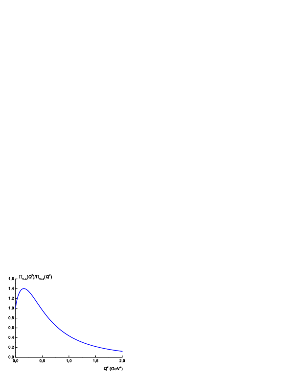
Figure 13: The ratio of the nonperturbative parts of the $V-A$ to $V+A$ correlators in the nonsinglet channel.

X Singlet axial vector current correlator and the topological susceptibility

The cancellations in the longitudinal channels are consequences of the current conservation and follow simply from the application of the nonanomalous Ward-Takahashi identities. We have explicitly demonstrated this in the previous Section in order to show the consistency of our calculations. The issue becomes important when we consider the longitudinal part of the isosinglet axial-vector current correlator which is not conserved due to the $U_{A}\left(1\right)$ axial Adler-Bell-Jackiw anomaly. This channel is dominated not by the pion, but by the $\eta^{\prime}$-meson intermediate state. Thus, in addition to the nonlocal interaction present in Eq. (18) we also need to include the interaction (21), where an exchange of the “$\eta$” singlet meson, the $SU(2)$ analog of the $\eta^{\prime}$ meson, occurs.

It is well known that due to the anomaly the singlet axial-vector current is not conserved even in the chiral limit,

$$\partial_{\mu}J_{\mu}^{50}\left(x\right)=2N_{f}Q_{5}\left(x\right),$$ (101)

where $Q_{5}\left(x\right)$ is the topological charge density. In QCD it is defined as $Q_{5}\left(x\right)=(\alpha_{s}/8\pi)G^{a}_{\mu\nu}(x)\tilde{G}^{a}_{\mu\nu}(x)$, where $G^{a}_{\mu\nu}$ is the gluonic field strength, and $\tilde{G}^{a}_{\mu\nu}$ is its dual, $\tilde{G}^{a}_{\mu\nu}=\varepsilon_{\mu\nu\lambda\sigma}G^{a}_{\lambda\sigma}$. The correlator of the singlet axial-vector currents has the same Lorentz structure as in Eq. (2), but without flavor indices and with $T^{a}\equiv 1$. In the chiral limit its longitudinal part is related to the topological susceptibility, the correlator of the topological charge densities $Q_{5}\left(x\right)$,

$$\chi\left(Q^{2}\right)=i\int d^{4}x~{}e^{iqx}\langle 0\left|T\left\{Q_{5}(x)Q_{5}(0)\right\}\right|0\rangle,$$ (102)

by the relation (see, e.g., IofSams00 )

$$\Pi_{L}^{A,0}\left(Q^{2}\right)=\frac{\left(2N_{f}\right)^{2}}{Q^{2}}\chi\left(Q^{2}\right).$$ (103)

At high $Q^{2}$ the OPE for $\chi\left(Q^{2}\right)$ predicts SVZeta

$$\chi\left(Q^{2}\rightarrow\infty\right)=-\frac{\alpha_{s}}{16\pi}\left\langle\frac{\alpha_{s}}{\pi}\left(G_{\mu\nu}^{a}\right)^{2}\right\rangle+\mathcal{O}(Q^{-2})+\mathcal{O}(e^{-Q\rho}),$$ (104)

where the perturbative contributions have been subtracted, and the exponential corrections are due to nonlocal instanton interactions IofSams00 .

At low $Q^{2}$ the topological susceptibility $\chi\left(Q^{2}\right)$ can be represented as a sum of contributions coming purely from QCD and from hadronic resonances, IofSams00 . Crewther proved the theorem Crew that $\chi\left(0\right)=0$ in any theory where at least one massless quark exists (the dependence of $\chi\left(0\right)$ on current quark masses has been found in Venez79 ). Also, the contributions of nonsinglet hadron resonances are absent in the chiral limit. Thus, in the low-$Q^{2}$ limit for massless current quarks one has

$$\left[\chi\left(Q^{2}\rightarrow 0\right)\right]_{\chi QCD}=-Q^{2}\chi^{\prime}(0)+\mathcal{O}(Q^{4}).$$ (105)

The estimates of $\chi^{\prime}(0)$ existing in the literature are rather controversial :

$$\chi^{\prime}(0)=\left(48\pm 6~{}\mathrm{MeV}\right)^{2}\qquad[69],\qquad\chi^{\prime}(0)=\left(26\pm 4~{}\mathrm{MeV}\right)^{2}\qquad[70].$$ (106)

This makes further model estimates valuable.

Now we turn to the model calculations. The bare isosinglet axial-vector current obtained from the interaction terms (19) and (21) by the rules described in Sect. IV becomes

$$\widetilde{\Gamma}_{\mu}^{50}(k,q,k^{\prime}=k+q) = \gamma_{\mu}\gamma_{5}-\gamma_{5}(k+k^{\prime})_{\mu}\frac{\left(\sqrt{M(k^{\prime})}-\sqrt{M(k)}\right)^{2}}{k^{\prime 2}-k^{2}}+$$

$$+ \gamma_{5}\frac{q_{\mu}}{q^{2}}2\sqrt{M(k^{\prime})M(k)}\left[\frac{G^{\prime}}{M_{q}^{2}}J_{AP}(q^{2})-\frac{G^{\prime}}{G}\right],$$

where $J_{AP}(q^{2})$is defined in Eq. (31). In order to get the full current we have to consider rescattering in the channel with the quantum numbers of the singlet pseudoscalar meson, “$\eta$”, which results in

$$\Gamma_{\mu}^{50}(k,q,k^{\prime}=k+q) = \gamma_{\mu}\gamma_{5}-\gamma_{5}(k+k^{\prime})_{\mu}\frac{\left(\sqrt{M(k^{\prime})}-\sqrt{M(k)}\right)^{2}}{k^{\prime 2}-k^{2}}$$

$$- \gamma_{5}\frac{q_{\mu}}{q^{2}}2\sqrt{M(k^{\prime})M(k)}\frac{G^{\prime}}{G}\frac{1-GJ_{PP}(q^{2})}{1-G^{\prime}J_{PP}(q^{2})}.$$

Because of the singlet axial anomaly this current does not contain the massless pole anymore, since according to Eq. (51) one has at zero momentum:

$$\frac{1-GJ_{PP}(q^{2})}{-q^{2}}=G\frac{f_{\pi}^{2}}{M_{q}^{2}}.$$ (109)

Instead, it develops a pole at the “$\eta$” meson mass. So, within the model considered the same mechanism is responsible for the sponteneous breaking of chiral symmetry and violation of the $U_{A}(1)$ symmetry.

The vertices satisfy the anomalous Ward-Takahashi identities:

$$q_{\mu}\widetilde{\Gamma}_{\mu}^{50}(k,q,k^{\prime}=k+q)=\widehat{q}\gamma_{5}-\gamma_{5}\left[M(k^{\prime})+M(k)\right]+\gamma_{5}2\sqrt{M(k^{\prime})M(k)}\left(1-\frac{G^{\prime}}{G}+G^{\prime}\frac{J_{AP}(q^{2})}{M_{q}^{2}}\right),$$ (110)

and

$$q_{\mu}\Gamma_{\mu}^{50}(k,q,k^{\prime}=k+q)=\widehat{q}\gamma_{5}-\gamma_{5}\left[M(k^{\prime})+M(k)\right]+\gamma_{5}\frac{2\sqrt{M(k^{\prime})M(k)}}{1-G^{\prime}J_{PP}(q^{2})}\left(1-\frac{G^{\prime}}{G}\right),$$ (111)

where the last term is due to the anomaly. Thus the QCD pseudoscalar gluonium operator is interpolated by the pseudoscalar effective quark field operator with coefficient expressed in terms of dynamical quark mass. In the effective quark model the connection between quark and integrated gluon degrees of freedom is fixed by the gap equation (23)DP85 . By considering the forward matrix element $(q=0)$ one deduces that the singlet axial constant is not renormalized within our scheme: $G_{A}^{(0)}(0)=1$. In order to get reduction of the singlet axial constant (“spin crisis”) we need to consider the effects of polarization of topologically neutral vacuum (see, e.g., Dorokhov:ym ).

It is instructive first to consider the longitudinal part of the correlator of the local vertex, $\gamma_{\mu}\gamma_{5}$, and the nonlocal vertex of Eq. (X), which is the construction of Pagels and Stokar pagsto79 . In this model the decay constant is defined by

$$f_{\pi,PS}^{2}=\frac{N_{c}}{8\pi^{2}}\int\limits_{0}^{\infty}du\ u\frac{2M(u)^{2}-uM(u)M^{\prime}(u)}{D^{2}\left(u\right)}.$$ (112)

Then, through the use of Eq. (103) we get for the topological susceptibility the result

$$\left(2N_{f}\right)^{2}\chi_{PS}\left(Q^{2}\right)=-\frac{G-G^{\prime}}{G\left[1-G^{\prime}J_{PP}(Q^{2})\right]}\frac{N_{c}N_{f}}{4\pi^{2}}\int d^{4}k\frac{\sqrt{M_{+}M_{-}}}{D_{+}D_{-}}\left[M_{+}\left(k_{-}q\right)-M_{-}\left(k_{+}q\right)\right],$$ (113)

with the coefficients of the low-$Q^{2}$ expansion given by

$$\chi_{PS}\left(0\right)=0,\qquad\chi_{PS}^{\prime}\left(0\right)=\frac{f_{\pi,PS}^{2}}{2N_{f}}.$$ (114)

Hence, the result is consistent with the Crewther theorem and it provides the estimate of $\chi_{PS}^{\prime}\left(0\right)\approx\left(39~{}\mathrm{MeV}\right)^{2}$ obtained for $N_{f}=3$. The second relation may be rewritten in the form resembling the generalized Goldberger-Treiman relation, as advocated by Veneziano and Shore NShVenez . Indeed, by using the standard Goldberger-Treiman relation, (48), valid in a given model, one finds

$$M_{q}=g_{\pi}^{PS}\sqrt{2N_{f}\chi_{PS}^{\prime}\left(0\right)},$$ (115)

which is just the quark-level relation from Ref. NShVenez . At large $Q^{2}$ the quantity $\chi_{PS}\left(Q^{2}\right)$ decreases according to the power of the dynamical quark form factor.

Now let us turn to the full model calculation. Proceeding in a similar manner as in the previous Sections we get the topological susceptibility in the form

$$-\left(2N_{f}\right)^{2}\chi\left(Q^{2}\right) = 2N_{f}\left(1-\frac{G^{\prime}}{G}\right)\left\{Q^{2}J_{\pi A}\left(Q^{2}\right)\left[1-\frac{G^{\prime}J_{AP}(Q^{2})}{M_{q}^{2}}+\frac{1}{1-G^{\prime}J_{PP}(Q^{2})}\right]\right.$$

$$+ M_{q}^{2}J_{PP}\left(Q^{2}\right)\left(1-\frac{G^{\prime}}{M_{q}^{2}}J_{AP}(Q^{2})\right)\left[\frac{GJ_{AP}(Q^{2})}{M_{q}^{2}}-\frac{G-G^{\prime}}{G\left[1-G^{\prime}J_{PP}(Q^{2})\right]}\right]$$

$$+ \left.\frac{G}{M_{q}^{2}}\left[4N_{c}N_{f}\int\frac{d^{4}k}{\left(2\pi\right)^{4}}\frac{M\left(k\right)}{D\left(k\right)}\left[M\left(k\right)-\sqrt{M\left(k+Q\right)M\left(k\right)}\right]\right]^{2}\right\},$$

where we have used the relation between the singlet current correlator and the topological susceptibility of Eq. (103). At large $Q^{2}$ one obtains the power-like behavior consistent with the OPE prediction (104), namely

$$-\left(2N_{f}\right)^{2}\chi\left(Q^{2}\rightarrow\infty\right)=\frac{2N_{f}M_{q}^{2}}{G}\left(1-\frac{G^{\prime}}{G}\right).$$ (117)

At zero momentum the topological susceptibility is zero

$$\chi\left(0\right)=0,$$ (118)

in accordance with the Crewther theorem. For the first moment of the topological susceptibility we obtain

$$\chi^{\prime}\left(0\right)=\frac{1}{2N_{f}}\left\{f_{\pi}^{2}\left(2-\frac{G^{\prime}}{G}\right)+\left(1-\frac{G^{\prime}}{G}\right)^{2}J_{AP}^{\prime}(0)\right\},$$ (119)

where $f_{\pi}^{2}$ and $J_{AP}^{\prime}(0)$ are defined in Eqs. (50) and (33), respectively.

In order to get numerical results we need to specify further the details of the model. We consider two possibilities. One involves the interaction with the exact symmetry as provided by the ’t Hooft determinant, $G^{\prime}=-G$. For the second possibility the constants $G$ and $G^{\prime}$ are considered as independent of each other, and their values are fixed with the help of the meson spectrum. In this more realistic scenario one has approximately the relation $G^{\prime}=0.1~{}G$ (for typical sets of parameters, c.f. Ref. Birse95 ). Then we get the following estimates for the first moment of the topological susceptibility:

$$\chi^{\prime}(0) = \left(55~{}\mathrm{MeV}\right)^{2}\qquad(G^{\prime}=-G),$$ (120)

$$\chi^{\prime}(0) = \left(50~{}\mathrm{MeV}\right)^{2}\qquad(G^{\prime}=0.1~{}G).$$ (121)

For the above estimates we have taken $N_{f}=3$. Since the flavor number enters only through the factor of $2N_{f}$ present in the definition (103), in this sense it is external to the model and its inclusion is very simple. We can see that the model gives the values of $\chi^{\prime}(0)$ which are close to the estimate of Ref. IoOg98 . In Fig. 3 we present the model predictions for the topological susceptibility at low and moderate values of $Q^{2}$ for the cases of the full (X) and Pagels-Stokar (113) model calculations.

We should note that the predictions of our model have a limited character because we have used the $SU_{f}\left(2\right)$ model in the chiral limit and have not considered mixing effects. However, our final result is formulated in terms of a physical observable, $f_{\pi}$, and thus we believe that the presented predictions may be not far from more realistic model calculations. In the region of small and intermediate momenta our results are quantitatively close to the predictions of the QCD sum rules with the instanton effects included IofSams00 . In our opinion, both the instanton-based calculations (our model with $\left(G^{\prime}=-G\right)$ and the interpolation of the model IofSams00 ) overestimate the instanton contributions in the region $Q^{2}\sim 0.5-2$ GeV². It would be interesting to verify the predictions given in Fig. 14 by the modern lattice simulations.

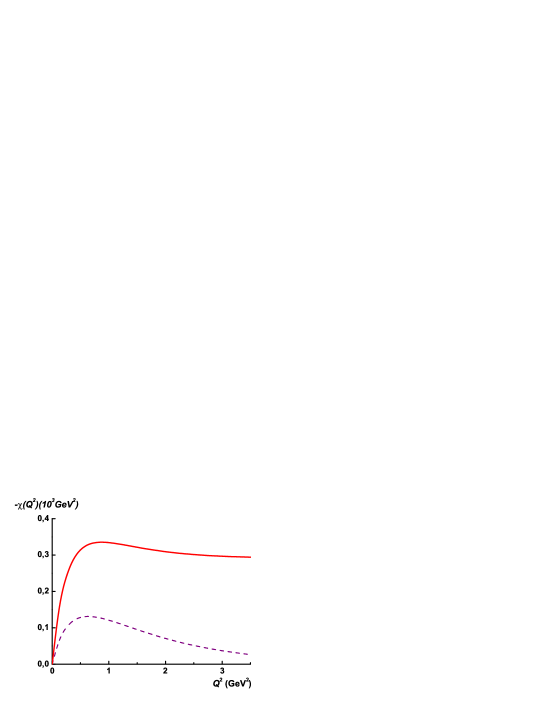
Figure 14: Topological susceptibility versus $Q^{2}$ predicted by the model with $G^{\prime}=0.1~{}G$, Eq. (X), (solid line), and by the Pagels-Stokar construction, Eq. (113) ,(dashed line).

XI Conclusions

In this work we have analyzed the nonperturbative parts of the Euclidean-momentum correlation functions of the vector and axial-vector currents within an effective nonlocal chiral quark model. To this end, we have derived the conserved vector and isotriplet axial-vector currents and demonstrated explicitly the absence of longitudinal parts in the $V$ and nonsinglet $A$ correlators, which is consequence of the gauge invariance of the present approach. On the other hand, the singlet $A$ correlator gains an anomalous contribution. From the properties of the $V-A$ correlator we have shown the fulfillment of the low-energy relations. The values of the $\pi^{\pm}-\pi^{0}$ electromagnetic mass difference and the electric pion polarizability are estimated and found to be remarkably close to the experimental values. In the high-energy region the relation to OPE has been discussed. In particular, the estimate of the $1/Q^{2}$ coefficient is in agreement with the recent lattice findings and the modified OPE phenomenology. We stress that the momentum dependence of the dynamical quark mass is crucial for the fulfillment of the second Weinberg sum rule. The combination $V-A$ receives no contribution from perturbative effects and provides a clean probe for chiral symmetry breaking and a test ground for model verification. We have found that our model describes well the transformed data of the ALEPH collaboration on the hadronic $\tau$ decay. The combination $V+A$, on the other hand, is dominated by perturbative contributions which are subtracted from our analysis. By considering the correlator of the singlet axial-vector currents the topological susceptibility has been found as a function of the momentum, and its first moment is predicted. In addition, the fulfillment of the Crewther theorem has been demonstrated.

- (1) R. Barate et al. [ALEPH Collaboration], Eur. Phys. J. C 4 (1998) 409; M. Davier, arXiv:hep-ex/0301035.
- (2) K. Ackerstaff et al. [OPAL Collaboration], Eur. Phys. J. C 7 (1999) 571.
- (3) S. Weinberg, Phys. Rev. Lett. 18 (1967) 507.
- (4) T. Das, V. S. Mathur and S. Okubo, Phys. Rev. Lett. 18 (1967) 761.
- (5) T. Das, G. S. Guralnik, V. S. Mathur, F. E. Low and J. E. Young, Phys. Rev. Lett. 18 (1967) 759.
- (6) J. Gasser and H. Leutwyler, Nucl. Phys. B 250 (1985) 465.
- (7) M. A. Shifman, A. I. Vainshtein and V. I. Zakharov, Nucl. Phys. B 147 (1979) 385.
- (8) K. G. Chetyrkin, S. Narison and V. I. Zakharov, Nucl. Phys. B 550 (1999) 353.
- (9) P. Boucaud, A. Le Yaouanc, J. P. Leroy, J. Micheli, O. Pene and J. Rodriguez-Quintero, Phys. Rev. D 63 (2001) 114003.
- (10) M. Davier, L. Girlanda, A. Hocker and J. Stern, Phys. Rev. D 58 (1998) 096014.
- (11) B. L. Ioffe and K. N. Zyablyuk, Nucl. Phys. A 687 (2001) 437; B. V. Geshkenbein, B. L. Ioffe and K. N. Zyablyuk, Phys. Rev. D 64 (2001) 093009.
- (12) B. V. Geshkenbein, “Hadronic tau decay, the renormalization group, analyticity of the polarization operators and QCD parameters,” arXiv:hep-ph/0206094.
- (13) T. Schafer and E. V. Shuryak, Phys. Rev. Lett. 86 (2001) 3973.
- (14) S. P. Klevansky and R. H. Lemmer, “Spectral density functions and their sum rules in an effective chiral field theory,” arXiv:hep-ph/9707206;
- (15) E. de Rafael, “Analytic approaches to kaon physics,” Plenary talk at 20th International Symposium on Lattice Field Theory (LATTICE 2002), Boston, Massachusetts, 24-29 Jun 2002, arXiv:hep-ph/0210317.
- (16) I. V. Anikin, A. E. Dorokhov and L. Tomio, Phys. Part. Nucl. 31 (2000) 509 [Fiz. Elem. Chast. Atom. Yadra 31 (2000) 1023].
- (17) S.V. Mikhailov, A.V. Radyushkin, Sov. J. Nucl. Phys. 49 (1989) 494 [Yad. Fiz. 49 (1988) 794]; Phys. Rev. D 45 (1992) 1754.
- (18) A. E. Dorokhov, S. V. Esaibegian and S. V. Mikhailov, Phys. Rev. D 56 (1997) 4062; Eur. Phys. J. C 13 (2000) 331.
- (19) D. Diakonov and V. Y. Petrov, Nucl. Phys. B 272 (1986) 457.
- (20) J. Terning, Phys. Rev. D 44 (1991) 887; B. Holdom, Phys. Rev. D 45 (1992) 2534.
- (21) H. Ito, W. Buck and F. Gross, Phys. Rev. C 43 (1991) 2483.
- (22) C. D. Roberts and A. G. Williams, Prog. Part. Nucl. Phys. 33 (1994) 477.
- (23) R. D. Bowler and M. C. Birse, Nucl. Phys. A 582 (1995) 655; R. S. Plant and M. C. Birse, Nucl. Phys. A 628 (1998) 607.
- (24) A. E. Dorokhov and L. Tomio, Phys. Rev. D 62 (2000) 014016.
- (25) W. Broniowski, “Mesons in non-local chiral quark models,” in Hadron Physics: Effective theories of low-energy QCD, Coimbra, Portugal, September 1999, AIP Conference Proceedings 508 (1999) 380, eds. A. H. Blin and B. Hiller and M. C. Ruivo and C. A. Sousa and E. van Beveren, AIP, Melville, New York, hep-ph/9911204.
- (26) W. Broniowski, Gauging non-local quark models, talk presented at the Mini-Workshop on Hadrons as Solitons, Bled, Slovenia, 6-17 July 1999, hep-ph/9909438.
- (27) B. Golli, W. Broniowski, and G. Ripka, Phys. Lett. B437 (1998) 24; W. Broniowski, B. Golli, and G. Ripka, Nucl. Phys. A703 (2002) 667.
- (28) M. Praszałowicz and A. Rostworowski, Phys. Rev. D64 (2001) 074003; Phys. Rev. D66 (2002) 054002.
- (29) I. V. Anikin, A. E. Dorokhov and L. Tomio, Phys. Lett. B 475 (2000) 361.
- (30) A. E. Dorokhov, JETP Letters, 77 (2003) 63 [Pisma ZHETF, 77 (2003) 68]; arXiv:hep-ph/0212156.
- (31) R. D. Ball and G. Ripka, in Many Body Physics (Coimbra 1993), edited by C. Fiolhais, M. Fiolhais, C. Sousa, and J. N. Urbano (World Scientific, Singapore, 1993).
- (32) E. R. Arriola and L. L. Salcedo, Phys. Lett. B450, 225 (1999).
- (33) D. Diakonov, Prog. Part. Nucl. Phys. 36, 1 (1996).
- (34) J. Bijnens, C. Bruno, and E. de Rafael, Nucl. Phys. B390, 501 (1993).
- (35) C. Christov, A. Blotz, H. Kim, P. Pobylitsa, T. Watabe, Th. Meissner, E. Ruiz Arriola, and K. Goeke, Prog. Part. Nucl. Phys. 37, 1 (1996).
- (36) E. Witten, Phys. Rev. Lett. 51 (1983) 2351.
- (37) C. Caso et al. [Particle Data Group Collaboration], Eur. Phys. J. C 3 (1998) 1.
- (38) S. R. Amendolia et al. [NA7 Collaboration], Nucl. Phys. B 277 (1986) 168.
- (39) S. Narison, QCD spectral sum rules, Lecture notes in physics, Vol. 26 (World Scientific, Singapore, 1989).
- (40) E. V. Shuryak, Nucl. Phys. B 203 (1982) 93.
- (41) E. V. Shuryak, Nucl. Phys. B 203 (1982) 116.
- (42) S. Narison and V. I. Zakharov, Phys. Lett. B 522 (2001) 266.
- (43) S. Mandelstam, Annals Phys. 19 (1962) 1.
- (44) D. Diakonov and V. Y. Petrov, Sov. Phys. JETP 62 (1985) 204 [Zh. Eksp. Teor. Fiz. 89 (1985) 361].
- (45) B. Holdom and R. Lewis, Phys. Rev. D 51 (1995) 6318.
- (46) K. Yamawaki and V.I. Zakharov, Extended Nambu-Jona-Lasinio model vs QCD sum rules.; hep-ph/9406373.
- (47) S. Peris and E. de Rafael, Nucl. Phys. B 500 (1997) 325.
- (48) H. Pagels and S. Stokar, Phys. Rev. D20 (1979) 2947.
- (49) J. S. Ball and T. W. Chiu, Phys. Rev. D 22 (1980) 2542.
- (50) L. Stodolsky, P. van Baal and V. I. Zakharov, Phys. Lett. B 552 (2003) 214.
- (51) D. Dudal, H. Verschelde, R. E. Browne and J. A. Gracey, arXiv:hep-th/0302128.
- (52) A. E. Dorokhov, N. I. Kochelev and Y. A. Zubov, Int. J. Mod. Phys. A 8 (1993) 603; A. E. Dorokhov, arXiv:hep-ph/0112332.
- (53) R. L. Jaffe and A. Manohar, Nucl. Phys. B 337 (1990) 509.
- (54) A. E. Dorokhov and W. Broniowski: Phys. Rev. D 65 (2002) 094007;
- (55) D. V. Shirkov and I. L. Solovtsov, Phys. Rev. Lett. 79 (1997) 1209.
- (56) S.B. Gerasimov, ”Meson structure constants in a model of the quark diagrams”, JINR-E2-11693, 1978; Yad. Fiz. 29 (1979) 513 [Sov. J. Nucl. Phys. 29, 259 (1979 ERRAT,32,156.1980)].
- (57) V.A. Petrunkin, Sov.J.Part.Nucl., 12 (1981) 278 [Fiz. Elem. Chast. Atom. Yadra 12 (1981) 692]
- (58) M.K. Volkov, Sov.J.Part.Nucl., 17 (1981) 185 [Fiz. Elem. Chast. Atom. Yadra 17 (1986) 433]; A. E. Dorokhov, M. K. Volkov, J. Hufner, S. P. Klevansky and P. Rehberg, Z. Phys. C 75 (1997) 127.
- (59) M.V. Terentev, Yad. Fiz. 16 (1972) 162 [Sov. J. Nucl. Phys., 16 (1972) 87].
- (60) U. Burgi, Nucl. Phys. B 479 (1996) 392.
- (61) S. P. Klevansky, R. H. Lemmer and C. A. Wilmot, Phys. Lett. B 457 (1999) 1.
- (62) M. Knecht, S. Peris and E. de Rafael, Phys. Lett. B 443 (1998) 255.
- (63) V. A. Andrianov and S. S. Afonin, Phys. Atom. Nucl. 65 (2002) 1862 [Yad. Fiz. 65 (2002) 1913].
- (64) B.L. Ioffe, arXiv:hep-ph/9811217; B.L. Ioffe, A.V. Samsonov, Phys. Atom. Nucl. 63 (2000) 1448 [Yad. Fiz. 63 (2000) 1527].
- (65) V.A. Novikov, M.A. Shifman, A.I. Vainshtein and V.I. Zakharov, Phys. Lett. B 86 (1979) 347.
- (66) G. Veneziano, Nucl. Phys. B 159 (1979) 213; P. Di Vecchia, G. Veneziano, Nucl. Phys. B 171 (1980) 253.
- (67) R.J. Crewther,Phys. Lett. B 70 (1977) 349.
- (68) K. Kawarabayashi and N. Ohta, Nucl. Phys. B 175 (1980) 477; Prog. Theor. Phys. 66 (1981) 1789.
- (69) B.L. Ioffe, A.G. Oganesian, Phys. Rev. D 57 (1998) 6590.
- (70) G.M. Shore, G. Veneziano, Phys. Lett. B 244 (1990) 75; S. Narison, G.M. Shore and G. Veneziano, Nucl. Phys. B 546 (1999) 235.
- (71) K. Fukushima, K. Ohnishi and K. Ohta, Phys. Rev. C 63 (2001) 045203; Phys. Lett. B 514 (2001) 200.