Heavy Baryonic Decays of $\Lambda_{b}\to\Lambda\eta^{(\prime)}$
and Nonspectator Contribution

Abstract

We calculate the branching ratios of the hadronic $\Lambda_{b}$ decays to $\eta$ and $\eta^{\prime}$ in the factorization approximation where the form factors are estimated via QCD sum rules and the pole model. Our results indicate that, contrary to $B\to K\eta^{(\prime)}$ decays, the branching ratios for $\Lambda_{b}\to\Lambda\eta$ and $\Lambda_{b}\to\Lambda\eta^{\prime}$ are more or less the same in the hadronic $\Lambda_{b}$ transitions. We estimate the branching ratio of $\Lambda_{b}\to\Lambda\eta^{(\prime)}$ to be $10.80(10.32)\times 10^{-6}$ in QCD sum rules, and $2.78(2.96)\times 10^{-6}$ in the pole model. We also estimate the nonfactorizable gluon fusion contribution to $\Lambda_{b}\to\Lambda\eta^{\prime}$ decay by dividing this process into strong and weak vertices. Our results point to an enhancement of more than an order of magnitude due to this mechanism.
PACS number(s): 13.30.Eg, 14.20.Mr, 14.40.Aq

I Introduction

For the last few years, different experimental groups have been accumulating plenty of data for the charmless hadronic $B$ decay modes. CLEO, Belle and BaBar Collaborations are providing us with the information on the branching ratio (BR) and the CP asymmetry for different decay modes. A clear picture is about to emerge from these information. Among the $B\to PP$ ($P$ denotes a pseudoscalar meson) decay modes, the BR for the decay $B^{+}\to K^{+}\eta^{\prime}$ is found to be larger than that expected within the standard model (SM). The observed BR for this mode in three different experiments are cleo ; belle ; babar

$${\mathcal{B}}(B^{\pm}\to K^{\pm}\eta^{\prime}) = (80^{+10}_{-9}\pm 7)\times 10^{-6}~{}~{}[{\rm CLEO}],$$ (1)

$$= (77.9^{+6.2+9.3}_{-5.9-8.7})\times 10^{-6}~{}~{}[{\rm Belle}],$$

$$= (67\pm 5\pm 5)\times 10^{-6}~{}~{}[{\rm BaBar}].$$

In order to explain the unexpectedly large branching ratio for $B\to K\eta^{\prime}$, different assumptions have been proposed, e.g., large form factors kagan , the QCD anomaly effect atwood ; ali1 , high charm content in $\eta^{\prime}$ halperin ; ali2 ; cheng1 , a new mechanism in the Standard Model du ; ahmady1 , the perturbative QCD approach kou , the QCD improved factorization approach beneke ; koy , or new physics like supersymmetry without R-parity choudhury ; dko1 ; dko2 . Even though some of these approaches turn out to be unsatisfactory, the other approaches are still waiting for being tested by experiment. Therefore, it would be much more desirable if besides using $B$ meson system, one can have an alternative way to test the proposed approaches in experiment.

Weak decays of the bottom baryon $\Lambda_{b}$ can provide a fertile testing ground for the SM. $\Lambda_{b}$ decays can also be used as an alternative and complimentary source of data to $B$ decays, because the underlying quark level processes are similar in both $\Lambda_{b}$ and $B$ decays. For example, $\Lambda_{b}\to\Lambda\eta^{(\prime)}$ decay involves similar quark level processes as $B\to K\eta^{(\prime)}$, i.e., $b\to q\bar{q}s$ ($q=u,~{}d,~{}s$). In the coming years, large number of $\Lambda_{b}$ baryons are expected to be produced in hadron machines, like Tevatron and LHC, and a high-luminosity linear collider running at the $Z$ resonance. For instance, the BTeV experiment, with a luminosity $2\times 10^{32}$ cm^-2 s^-1, is expected to produce $2\times 10^{11}$ $b\bar{b}$ hadrons per $10^{7}$ seconds stone , which would result in the production of $2\times 10^{10}$ $\Lambda_{b}$ baryons per year of running giri . One of peculiar properties of $\Lambda_{b}$ decays is that, unlike $B$ decays, these decays can provide valuable information about the polarization of the $b$ quark. Experimentally the polarization of $\Lambda_{b}$ has been measured aod .

In this work, we study $\Lambda_{b}\to\Lambda\eta^{(\prime)}$ decay. Our goal is two-fold: (i) The calculation of the BR for $\Lambda_{b}\to\Lambda\eta^{(\prime)}$ involves hadronic form factors which are highly model-dependent. Using different models for the form factors, we calculate the BR for $\Lambda_{b}\to\Lambda\eta^{(\prime)}$ and investigate the model-dependence of the theoretical prediction. (ii) As an alternative test for a possible mechanism explaining the large BR for $B^{+}\to K^{+}\eta^{\prime}$, we examine the same mechanism using $\Lambda_{b}\to\Lambda\eta^{\prime}$ decay. Among the mechanisms proposed for understanding the large ${\cal B}(B^{+}\to K^{+}\eta^{\prime})$, we focus on a nonspectator mechanism presented in Refs. du ; ahmady1 . In this mechanism, $\eta^{\prime}$ is produced via the fusion of two gluons: one from the QCD penguin diagram $b\to sg^{*}$ and the other one emitted by the light quark inside the $B$ meson. We calculate this nonspectator contribution to the BR for $\Lambda_{b}\to\Lambda\eta^{\prime}$ in order to examine its validity. If this nonspectator process is indeed the true mechanism responsible for the large ${\cal B}(B^{+}\to K^{+}\eta^{\prime})$, then the same mechanism would affect ${\cal B}(\Lambda_{b}\to\Lambda\eta^{\prime})$ as well. Thus, one can test the validity of this mechanism in the future experiments such as BTeV, LHC-b, etc., by comparing ${\cal B}(\Lambda_{b}\to\Lambda\eta^{\prime})$ calculated with/without the nonspectator contribution with the measured results.

We organize our work as follows. In Sec. II, we present the effective Hamiltonian for the usual $\Delta B=1$ transition and for the nonspectator process. We calculate the BR for $\Lambda_{b}\to\Lambda\eta^{(\prime)}$ decay without considering the nonspectator mechanism in Sec. III. The nonspectator contribution to $\Lambda_{b}\to\Lambda\eta^{\prime}$ is estimated in Sec. IV. We conclude in Sec. V.

II Effective Hamiltonian for $\Lambda_{b}\to\Lambda\eta^{(\prime)}$ decays

The effective Hamiltonian $H_{\rm eff}$ for the $\Delta B=1$ transition is

$$H_{\rm eff} = \frac{4G_{F}}{\sqrt{2}}\bigg{[}V_{ub}V^{\ast}_{uq}(c_{1}O_{1u}^{q}+c_{2}O_{2u}^{q})+V_{cb}V^{\ast}_{cq}(c_{1}O_{1c}^{q}+c_{2}O_{2c}^{q})$$ (2)

$$\hskip 28.45274pt-V_{tb}V^{\ast}_{tq}\sum_{i=3}^{12}c_{i}O_{i}^{q}\bigg{]}+h.c.,$$

where $q=d~{}{\rm or}~{}s$, and

$$O_{1f}^{q}=\bar{q}_{\alpha}\gamma_{\mu}Lf_{\alpha}\bar{f}_{\beta}\gamma^{\mu}Lb_{\beta},~{}~{}O_{2f}^{q}=\bar{q}_{\alpha}\gamma_{\mu}Lf_{\beta}\bar{f}_{\beta}\gamma^{\mu}Lb_{\alpha},$$

$$O_{3(5)}^{q}=\bar{q}_{\alpha}\gamma_{\mu}Lb_{\alpha}\sum_{q^{\prime}}\bar{q^{\prime}}_{\beta}\gamma^{\mu}L(R)q^{\prime}_{\beta},~{}~{}O_{4(6)}^{q}=\bar{q}_{\alpha}\gamma_{\mu}Lb_{\beta}\sum_{q^{\prime}}\bar{q^{\prime}}_{\beta}\gamma^{\mu}L(R)q^{\prime}_{\alpha},$$

$$O_{7(9)}^{q}=\frac{3}{2}\bar{q}_{\alpha}\gamma_{\mu}Lb_{\alpha}\sum_{q^{\prime}}e_{q^{\prime}}\bar{q^{\prime}}_{\beta}\gamma^{\mu}R(L)q^{\prime}_{\beta},~{}~{}O_{8(10)}^{q}=\frac{3}{2}\bar{q}_{\alpha}\gamma_{\mu}Lb_{\beta}\sum_{q^{\prime}}e_{q^{\prime}}\bar{q^{\prime}}_{\beta}\gamma^{\mu}R(L)q^{\prime}_{\alpha},$$

$$O_{11}=\frac{g_{s}}{32\pi^{2}}m_{b}\bar{q}\sigma^{\mu\nu}RT^{a}bG^{a}_{\mu\nu},~{}~{}O_{12}=\frac{e}{32\pi^{2}}m_{b}\bar{q}\sigma^{\mu\nu}RbF_{\mu\nu},$$ (3)

with $f=u~{}{\rm or}~{}c$ and $q^{\prime}=u,d,s,c$ and $L(R)=(1\mp\gamma_{5})/2$. The SU(3) generator $T^{a}$ is normalized as ${\rm Tr}(T^{a}T^{b})=\frac{1}{2}\delta^{ab}$. $\alpha$ and $\beta$ are the color indices. $G^{\mu\nu}_{a}$ and $F^{\mu\nu}$ are the gluon and photon field strength, and $c_{i}$’s are the Wilson coefficients (WCs). We use the improved effective WCs given in Refs. chen ; hou . The renormalization scale is taken to be $\mu=m_{b}$ ddo . The operators $O_{1}$, $O_{2}$ are the tree level and QCD corrected operators, $O_{3-6}$ are the gluon induced strong penguin operators, and finally $O_{7-10}$ are the electroweak penguin operators due to $\gamma$ and $Z$ exchange, and the box diagrams at loop level. In this work we shall take into account the chromomagnetic operator $O_{11}$, but neglect the extremely small contribution from $O_{12}$.

Considering the gluon splits into two quarks, the chomomagnetic operator is rewritten in the Fierz transformed form as

$$O_{11}=\frac{\alpha_{s}}{16\pi}\frac{m_{b}^{2}}{k^{2}}\frac{N_{c}^{2}-1}{N_{c}^{2}}\left[\delta_{\alpha\beta}\delta_{\alpha^{\prime}\beta^{\prime}}-\frac{2N_{c}}{N_{c}^{2}-1}T_{\alpha\beta}^{a}T_{\alpha^{\prime}\beta^{\prime}}^{a}\right]\sum_{i=1}^{4}T_{i},$$ (4)

where

$$T_{1} = 2\bar{s}_{\alpha}\gamma^{\mu}Lq^{\prime}_{\beta}\bar{q^{\prime}}_{\alpha^{\prime}}\gamma_{\mu}Lb_{\beta^{\prime}}-4\bar{s}_{\alpha}Rq^{\prime}_{\beta}\bar{q^{\prime}}_{\alpha^{\prime}}Lb_{\beta^{\prime}},$$

$$T_{2} = \frac{m_{s}}{m_{b}}(2\bar{s}_{\alpha}\gamma^{\mu}Rq^{\prime}_{\beta}\bar{q^{\prime}}_{\alpha^{\prime}}\gamma_{\mu}Rb_{\beta^{\prime}}-4\bar{s}_{\alpha}Lq^{\prime}_{\beta}\bar{q^{\prime}}_{\alpha^{\prime}}Rb_{\beta^{\prime}},$$

$$T_{3} = \frac{(p_{b}+p_{s})_{\mu}}{m_{b}}[\bar{s}_{\alpha}\gamma^{\mu}Lq^{\prime}_{\beta}\bar{q^{\prime}}_{\alpha^{\prime}}Rb_{\beta^{\prime}}+\bar{s}_{\alpha}Rq^{\prime}_{\beta}\bar{q^{\prime}}_{\alpha^{\prime}}\gamma^{\mu}Rb_{\beta^{\prime}}],$$

$$T_{4} = i\frac{(p_{b}+p_{s})_{\mu}}{m_{b}}[\bar{s}_{\alpha}\sigma^{\mu\nu}Rq^{\prime}_{\beta}\bar{q^{\prime}}_{\alpha^{\prime}}\gamma_{\nu}Rb_{\beta^{\prime}}-\bar{s}_{\alpha}\gamma_{\nu}Lq^{\prime}_{\beta}\bar{q^{\prime}}_{\alpha^{\prime}}\sigma^{\mu\nu}Rb_{\beta^{\prime}}].$$ (5)

Here $p_{b}$ and $p_{s}$ are the four-momenta of $b$- and $s$-quarks, respectively. $N_{c}$ denotes the effective number of colors and $k\equiv p_{b}-p_{s}$ is the gluon momentum. In the heavy quark limit, $k^{2}=m_{b}^{2}(1-x)$, where $x$ is the momentum fraction of $\eta^{(\prime)}$. The average gluon momentum can be estimated bensalem as

$$\left\langle\frac{m_{b}^{2}}{k^{2}}\right\rangle=\int_{0}^{1}(\phi_{\eta^{(\prime)}}(x)m_{b}^{2}/k^{2})dx,$$ (6)

where $\phi_{\eta^{(\prime)}}$ is the $\eta^{(\prime)}$ light-cone distribution and its asymptotic form is $\phi_{\eta^{(\prime)}}=6x(1-x)$.

The effective Hamiltonian for the nonspectator contribution can be obtained by considering the dominant chromo-electric component of the QCD penguin diagram ahmady1 ; ahmady2 :

$$H_{\rm nonsp}=iCH[\bar{s}\gamma^{\mu}(1-\gamma_{5})T^{a}b](\bar{q}\gamma^{\nu}T^{a}q){1\over p_{2}^{2}}\epsilon_{\mu\nu\rho\sigma}p_{1}^{\rho}p_{2}^{\sigma}~{},$$ (7)

where

$$C={G_{F}\over\sqrt{2}}{\alpha_{s}\over 2\pi}V_{tb}V^{*}_{ts}[E(x_{t})-E(x_{c})]~{},$$ (8)

$q$ denotes the spectator quark, and $p_{i}$ $(i=1,2)$ are the four-momenta of the two gluons relevant to the $g-g-\eta^{\prime}$ vertex. The coefficient function $E$ is defined as

$$E(x_{i})=-{2\over 3}{\rm ln}x_{i}+{x^{2}_{i}(15-16x_{i}+4x_{i}^{2})\over 6(1-x_{i})^{4}}{\rm ln}x_{i}+{x_{i}(18-11x_{i}-x_{i}^{2})\over 12(1-x_{i})^{3}}~{},$$ (9)

where $x_{i}=m_{i}^{2}/m_{W}^{2}$ with $m_{i}$ being the internal quark mass. $H$ is the form factor parametrizing the $g-g-\eta^{\prime}$ vertex

$$A_{\mu\nu}(gg\to\eta^{\prime})=iH(p_{1}^{2},p_{2}^{2},m_{\eta^{\prime}}^{2})\delta^{ab}\epsilon_{\mu\nu\rho\sigma}p_{1}^{\rho}p_{2}^{\sigma}~{}.$$ (10)

Using the decay mode $\psi\to\eta^{\prime}\gamma$, $H(0,0,m_{\eta^{\prime}}^{2})$ is estimated to be approximately 1.8 GeV^-1.

III $\Lambda_{b}\to\Lambda\eta^{(\prime)}$ Decay Process within Factorization Approach

In general, the vector and axial-vector matrix elements for the $\Lambda_{b}\to\Lambda$ transition can be parameterized as

$$\langle\Lambda|\bar{s}\gamma_{\mu}b|\Lambda_{b}\rangle = \bar{u}_{\Lambda}\left[f_{1}\gamma_{\mu}+i\frac{f_{2}}{m_{\Lambda_{b}}}\sigma_{\mu\nu}q^{\nu}+\frac{f_{3}}{m_{\Lambda_{b}}}q_{\mu}\right]u_{\Lambda_{b}},$$

$$\langle\Lambda|\bar{s}\gamma_{\mu}\gamma_{5}b|\Lambda_{b}\rangle = \bar{u}_{\Lambda}\left[g_{1}\gamma_{\mu}\gamma_{5}+i\frac{g_{2}}{m_{\Lambda_{b}}}\sigma_{\mu\nu}q^{\nu}\gamma_{5}+\frac{g_{3}}{m_{\Lambda_{b}}}q_{\mu}\gamma_{5}\right]u_{\Lambda_{b}},$$ (11)

where the momentum transfer $q^{\mu}=p^{\mu}_{\Lambda_{b}}-p^{\mu}_{\Lambda}$ and $f_{i}$ and $g_{i}(i=1,2,3)$ are Lorentz invariant form factors. Alternatively, with the HQET, the hadronic matrix elements for the $\Lambda_{b}\to\Lambda$ transition can be parameterized mannel as

$$\langle\Lambda|\bar{s}\Gamma b|\Lambda_{b}\rangle=\bar{u}_{\Lambda}\left[F_{1}(q^{2})+v/\hskip 0.85358ptF_{2}(q^{2})\right]\Gamma u_{\Lambda_{b}},$$ (12)

where $v=p_{\Lambda_{b}}/m_{\Lambda_{b}}$ is the four-velocity of $\Lambda_{b}$ and $\Gamma$ denotes the possible Dirac matrix. The relations between $f_{i},g_{i}$ and $F_{i}$ can be easily given by

$$f_{1}=g_{1}=F_{1}+rF_{2},~{}~{}f_{2}=f_{3}=g_{2}=g_{3}=F_{2},$$ (13)

where $r=m_{\Lambda}/m_{\Lambda_{b}}$.

The decay constants of the $\eta$ and $\eta^{\prime}$ mesons, $f^{q}_{\eta^{(\prime)}}$, are defined by

$$\langle 0|\bar{q}\gamma^{\mu}\gamma_{5}q|\eta^{(\prime)}\rangle=if^{q}_{\eta^{(\prime)}}p^{\mu}_{\eta^{(\prime)}}~{}~{}~{}(q=u,s).$$ (14)

Due to the $\eta-\eta^{\prime}$ mixing, the decay constants of the physical $\eta$ and $\eta^{\prime}$ are related to those of the flavor SU(3) singlet state $\eta_{0}$ and octet state $\eta_{8}$ through the relations leut ; feldmann

$$f^{u}_{\eta} = {f_{8}\over\sqrt{6}}\cos\theta_{8}-{f_{0}\over\sqrt{3}}\sin\theta_{0}~{},~{}~{}f^{s}_{\eta}=-2{f_{8}\over\sqrt{6}}\cos\theta_{8}-{f_{0}\over\sqrt{3}}\sin\theta_{0}~{},$$

$$f^{u}_{\eta^{\prime}} = {f_{8}\over\sqrt{6}}\sin\theta_{8}+{f_{0}\over\sqrt{3}}\cos\theta_{0}~{},~{}~{}f^{s}_{\eta^{\prime}}=-2{f_{8}\over\sqrt{6}}\sin\theta_{8}+{f_{0}\over\sqrt{3}}\cos\theta_{0}~{},$$ (15)

where $\theta_{8}$ and $\theta_{0}$ are the mixing angles and phenomenologically $\theta_{8}=-21.2^{0}$ and $\theta_{0}=-9.2^{0}$ feldmann . We use $f_{8}=166$ MeV and $f_{0}=154$ MeV chen .

The decay amplitude of $\Lambda_{b}\to\Lambda\eta^{\prime}$ is given bensalem by

$$\langle\Lambda\eta^{\prime}|H_{\rm eff}|\Lambda_{b}\rangle = \frac{4G_{F}}{\sqrt{2}}\bigg{[}V_{ub}V_{us}^{\ast}a_{2}\langle\eta^{\prime}|\bar{u}\gamma^{\mu}Lu|0\rangle\langle\Lambda|\bar{s}\gamma_{\mu}Lb|\Lambda_{b}\rangle$$ (16)

$$\hskip 14.22636pt-V_{tb}V_{ts}^{\ast}\left(2a_{3}-2a_{5}-\frac{1}{2}a_{7}+\frac{1}{2}a_{9}\right)\langle\eta^{\prime}|\bar{u}\gamma^{\mu}Lu|0\rangle\langle\Lambda|\bar{s}\gamma_{\mu}Lb|\Lambda_{b}\rangle$$

$$\hskip 14.22636pt-V_{tb}V_{ts}^{\ast}\left\{a_{3}+a_{4}-a_{5}+\frac{1}{2}a_{7}-\frac{1}{2}a_{9}+\left(1+\frac{2p_{b}\cdot q}{m_{b}^{2}}\right)a_{f}\right\}$$

$$\hskip 56.9055pt\times\langle\eta^{\prime}|\bar{s}\gamma^{\mu}Ls|0\rangle\langle\Lambda|\bar{s}\gamma_{\mu}Lb|\Lambda_{b}\rangle$$

$$\hskip 14.22636pt-V_{tb}V_{ts}^{\ast}\chi_{\eta^{\prime}}\left(-a_{6}+\frac{1}{2}a_{8}-\frac{5}{4}a_{f}\right)\langle\eta^{\prime}|\bar{u}\gamma^{\mu}Lu|0\rangle\langle\Lambda|\bar{s}\gamma_{\mu}Rb|\Lambda_{b}\rangle$$

$$\hskip 14.22636pt-V_{tb}V_{ts}^{\ast}\chi_{\eta^{\prime}}\left(a_{6}-\frac{1}{2}a_{8}+\frac{5}{4}a_{f}\right)\langle\eta^{\prime}|\bar{s}\gamma^{\mu}Ls|0\rangle\langle\Lambda|\bar{s}\gamma_{\mu}Rb|\Lambda_{b}\rangle\bigg{]},$$

where

$$a_{i} \equiv c_{i}^{\rm eff}+\frac{1}{N_{c}}c_{i+1}^{\rm eff}~{}~{}~{}({\rm for}~{}i={\rm odd}),$$

$$a_{i} \equiv c_{i}^{\rm eff}+\frac{1}{N_{c}}c_{i-1}^{\rm eff}~{}~{}~{}({\rm for}~{}i={\rm even}),$$

$$\chi_{\eta^{\prime}} = \frac{m_{\eta^{\prime}}^{2}}{m_{b}m_{s}},$$

$$a_{f} = \frac{\alpha_{s}}{16\pi k^{2}}m_{b}^{2}\frac{N_{c}^{2}-1}{N_{c}^{2}}c_{11}.$$ (17)

In the above amplitude, we have taken into account the anomaly contribution to the matrix element $\langle\eta^{\prime}|\bar{s}\gamma_{5}s|0\rangle$ ali2 ; ddo ; ball ; cheng2 , which leads to

$$\langle\eta^{\prime}|\bar{s}\gamma_{5}s|0\rangle=i{(f^{s}_{\eta^{\prime}}-f^{u}_{\eta^{\prime}})m^{2}_{\eta^{\prime}}\over 2m_{s}}~{}.$$ (18)

The similar expression for the decay amplitude of $\Lambda_{b}\to\Lambda\eta$ can be obtained by replacing $\eta^{\prime}$ by $\eta$ in the above Eq. (16).

The decay amplitude given in Eq. (16) can be rewritten in the general form

$${\cal M}\equiv\langle\Lambda\eta^{\prime}|H_{\rm eff}|\Lambda_{b}\rangle=i\bar{u}_{\Lambda}(a+b\gamma_{5})u_{\Lambda_{b}}.$$ (19)

The averaged square of the amplitude is

$$\overline{|{\cal M}|^{2}}=2(|a|^{2}-|b|^{2})m_{\Lambda}m_{\Lambda_{b}}+2(|a|^{2}+|b|^{2})p_{\Lambda}\cdot p_{\Lambda_{b}},$$ (20)

where

$$a = (X+Y)\left[(m_{\Lambda_{b}}-m_{\Lambda})f_{1}+\frac{m_{\eta^{\prime}}^{2}}{m_{\Lambda_{b}}}f_{3}\right],$$

$$b = (X-Y)\left[(m_{\Lambda_{b}}-m_{\Lambda})g_{1}-\frac{m_{\eta^{\prime}}^{2}}{m_{\Lambda_{b}}}g_{3}\right],$$

$$X = \frac{G_{F}}{\sqrt{2}}\bigg{[}\Big{\{}V_{ub}V_{us}^{\ast}a_{2}-V_{tb}V_{ts}^{\ast}\Big{(}2a_{3}-2a_{5}-\frac{1}{2}a_{7}+\frac{1}{2}a_{9}\Big{)}\Big{\}}f_{\eta^{\prime}}^{u}$$

$$\hskip 18.49428pt-V_{tb}V_{ts}^{\ast}\Big{\{}a_{3}+a_{4}-a_{5}+\frac{1}{2}a_{7}-\frac{1}{2}a_{9}+\Big{(}1+\frac{2p_{b}\cdot q}{m_{b}^{2}}\Big{)}a_{f}\Big{\}}f_{\eta^{\prime}}^{s}\bigg{]},$$

$$Y = \frac{G_{F}}{\sqrt{2}}V_{tb}V_{ts}^{\ast}\chi_{\eta^{\prime}}\Big{(}a_{6}-\frac{1}{2}a_{8}+\frac{5}{4}a_{f}\Big{)}(f_{\eta^{\prime}}^{u}-f_{\eta^{\prime}}^{s}).$$ (21)

Then the decay width of $\Lambda_{b}\to\Lambda\eta^{\prime}$ in the rest frame of $\Lambda_{b}$ is given by

$$\Gamma(\Lambda_{b}\to\Lambda\eta^{\prime})=\frac{1}{16\pi m_{\Lambda_{b}}}\lambda^{\frac{1}{2}}\bigg{(}1,\frac{m_{\Lambda}^{2}}{m_{\Lambda_{b}}^{2}},\frac{m_{\eta^{\prime}}^{2}}{m_{\Lambda_{b}}^{2}}\bigg{)}\sum|{\cal M}|^{2},$$ (22)

where

$$\lambda(1,a,b)=1+a^{2}+b^{2}-2a-2b-2ab.$$ (23)

For numerical calculations, we need specific values for the form factors in the $\Lambda_{b}\to\Lambda$ transition which are model-dependent. We use the values of the form factors from both the QCD sum rule approach huang and the pole model mannel ; geng . In the QCD sum rule approach, the form factors $F_{1}$ and $F_{2}$ are given by

$$F_{1} = -{e^{2\bar{\Lambda}/M+m_{\Lambda}^{2}/T}\over 2f_{\Lambda_{b}}f_{\Lambda}}\int^{\nu_{c}}_{0}d\nu\int^{2\nu z}_{0}ds\rho^{1}_{pert}e^{-s/T-\nu/M}-{1\over 3}\langle\bar{q}q\rangle^{2}$$

$$-{1\over 32\pi^{4}}\langle\alpha_{s}GG\rangle\int^{T/4}_{0}\left(1-{4\beta\over T}\right)e^{-4\beta(1-4\beta/T)/M^{2}-8\beta z/(TM)}d\beta,$$

$$F_{2} = -{e^{2\bar{\Lambda}/M+m_{\Lambda}^{2}/T}\over 2f_{\Lambda_{b}}f_{\Lambda}}\int^{\nu_{c}}_{0}d\nu\int^{2\nu z}_{0}ds\rho^{2}_{pert}e^{-s/T-\nu/M}$$ (24)

$$+{1\over 8\pi^{4}}\langle\alpha_{s}GG\rangle\int^{T/4}_{0}\left(1-{4\beta\over T}\right){\beta\over M}e^{-4\beta(1-4\beta/T)/M^{2}-8\beta z/(TM)}d\beta,$$

where

$$\rho^{1}_{pert} = {1\over 32\pi^{4}\sigma^{3}}\{-2z^{3}\sigma^{3}-[-s+z(\nu+2z)]^{3}+3z^{2}[-s+z(\nu+2z)]\sigma^{2}\},$$

$$\rho^{2}_{pert} = -{1\over 64\pi^{4}\sigma^{3}}[s-2z^{2}+z(-\nu+\sigma)]^{2}[\nu s+8z^{3}-4z^{2}(-2\nu+\sigma)-2z(-\nu^{2}+5s+\nu\sigma)],$$

$$\sigma = \sqrt{-4s+(\nu+2z)^{2}}~{}.$$ (25)

Here $z=\frac{p_{\Lambda}\cdot p_{\Lambda_{b}}}{m_{\Lambda_{b}}}=\frac{m_{\Lambda_{b}}^{2}+m_{\Lambda}^{2}-q^{2}}{2m_{\Lambda_{b}}}$ $(q^{\mu}=p_{\Lambda_{b}}^{\mu}-p_{\Lambda}^{\mu})$ and the Borel parameter $M=\frac{4T}{m_{b}}$. For the other relevant conventions and notation, we refer to Ref. huang . In Figs. 1 and 2 we show the form factors $F_{1}$ and $F_{2}$ as a function of the Borel parameter $M={4T\over m_{b}}$ for $\Lambda_{b}\to\Lambda\eta^{(^{\prime})}$, respectively. In $\Lambda_{b}\to\Lambda\eta^{(^{\prime})}$, $F_{1}=0.510(0.514)$ and $F_{2}=-0.058(-0.060)$ for $M=1.5$, $F_{1}=0.476(0.481)$ and $F_{2}=-0.084(-0.088)$ for $M=1.7$, and $F_{1}=0.473(0.479)$ and $F_{2}=-0.117(-0.122)$ for $M=1.9$ . The BRs of $\Lambda_{b}\to\Lambda\eta^{\prime}$ and $\Lambda_{b}\to\Lambda\eta$ versus $\xi\equiv{1\over N_{c}}$ for different values of the Borel parameter $M={4T\over m_{b}}$ are shown in Fig. 3 and Fig. 4, respectively. Our result shows

$${\cal B}(\Lambda_{b}\to\Lambda\eta^{\prime})=(5.0-14.5)\times 10^{-6}~{},$$ (26)

and

$${\cal B}(\Lambda_{b}\to\Lambda\eta)=(5.8-13.7)\times 10^{-6}~{}.$$ (27)

For $\xi=1/3~{}({\rm i.e.,}~{}N_{c}=3)$ and $M=1.7$ GeV, ${\cal B}(\Lambda_{b}\to\Lambda\eta^{\prime})=8.93\times 10^{-6}$ and ${\cal B}(\Lambda_{b}\to\Lambda\eta)=9.15\times 10^{-6}$. We recall that in the case of $B\to K\eta^{\prime}$ a small value of $\xi$ ($\xi\leq 0.1$) is favored to fit the experimental data on the BR in the framework of the generalized factorization ali2 ; chen ; ddo ; cheng2 . In the figures the shaded region denotes the case of $\xi\leq 0.1$ , favored from the analysis of $B\to K\eta^{\prime}$. For $\xi=0.1$, ${\cal B}(\Lambda_{b}\to\Lambda\eta^{\prime})=11.17\times 10^{-6}$ and ${\cal B}(\Lambda_{b}\to\Lambda\eta)=10.83\times 10^{-6}$.

Figure 1: The form factor $F_{1}$ for the transition $\Lambda_{b}\to\Lambda$ versus the Borel parameter $M~{}(={4T\over m_{b}})$. The dotted (solid) line corresponds to the case of $\Lambda_{b}\to\Lambda\eta^{(^{\prime})}$.

Figure 2: The form factor $F_{2}$ for the transition $\Lambda_{b}\to\Lambda$ versus the Borel parameter $M~{}(={4T\over m_{b}})$. The dotted (solid) line corresponds to the case of $\Lambda_{b}\to\Lambda\eta^{(^{\prime})}$.

We note that the BR of $\Lambda_{b}\to\Lambda\eta$ is similar to that of $\Lambda_{b}\to\Lambda\eta^{\prime}$, in contrast to the case of $B\to K\eta^{(^{\prime})}$ where the BR of $B\to K\eta$ is about an order of magnitude smaller than that of $B\to K\eta^{\prime}$. This difference mainly arises from the fact that in the factorization scheme, the decay amplitude for $\Lambda_{b}\to\Lambda\eta^{(^{\prime})}$ consists of terms proportional to $\langle\eta^{(^{\prime})}|O|0\rangle\langle\Lambda|O^{\prime}|\Lambda_{b}\rangle$ only (see Eq. (16)), while the decay amplitude for $B\to K\eta^{(^{\prime})}$ consists of terms proportional to $\langle K|\tilde{O}|0\rangle\langle\eta^{(^{\prime})}|\tilde{O}^{\prime}|B\rangle$ as well as terms proportional to $\langle\eta^{(^{\prime})}|O|0\rangle\langle K|O^{\prime}|B\rangle$ ali2 ; chen ; ddo . (Here $O^{(^{\prime})}$ and $\tilde{O}^{(^{\prime})}$ denote the relevant quark currents arising from the effective Hamiltonian (2).) In the case of $B\to K\eta^{(^{\prime})}$, the destructive (constructive) interference appears between the penguin amplitude proportional to $\langle K|\tilde{O}|0\rangle\langle\eta^{(^{\prime})}|\tilde{O}^{\prime}|B\rangle$ and that proportional to $\langle\eta^{(^{\prime})}|O|0\rangle\langle K|O^{\prime}|B\rangle$, due to the opposite (same) sign between $\langle K|\tilde{O}|0\rangle\propto f_{K}$ and $\langle\eta^{(^{\prime})}|O|0\rangle\propto f^{q}_{\eta^{(^{\prime})}}$: in particular, $f^{s}_{\eta}=-112$ MeV, while $f^{s}_{\eta^{\prime}}=+137$ MeV (see Eq. (15)). However, in the case of $\Lambda_{b}\to\Lambda\eta^{(^{\prime})}$, there is no such interference between terms in the amplitude because the amplitude contains terms proportional to $\langle\eta^{(^{\prime})}|O|0\rangle\propto f^{q}_{\eta^{(^{\prime})}}$ only.

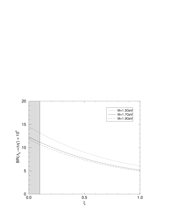
Figure 3: The BR for the decay $\Lambda_{b}\to\Lambda\eta^{\prime}$ versus $\xi={1\over N_{c}}$ for different values of the Borel parameter $M={4T\over m_{b}}$. The shaded region denotes the case of $\xi\leq 0.1$, which is favored from the analysis of $B\to K\eta^{\prime}$ decays.

Figure 4: The BR for the decay $\Lambda_{b}\to\Lambda\eta$ versus $\xi={1\over N_{c}}$ for different values of the Borel parameter $M={4T\over m_{b}}$. The shaded region denotes the case of $\xi\leq 0.1$, which is favored from the analysis of $B\to K\eta^{\prime}$ decays.

In the pole model mannel ; geng , the form factors are given by

$$F_{i}(q^{2})=N_{i}\left(\frac{\Lambda_{\rm QCD}}{\Lambda_{\rm QCD}+z}\right)^{2}~{},~{}~{}(i=1,2)$$ (28)

where $\Lambda_{\rm QCD}\sim$ 200 MeV and $z=\frac{p_{\Lambda}\cdot p_{\Lambda_{b}}}{m_{\Lambda_{b}}}$. Using $N_{1}=52.32$ and $N_{2}=-13.08$ , we obtain the values of the form factors: $F_{1}(q^{2})=0.225~{}(0.217)$ and $F_{2}(q^{2})=-0.056~{}(-0.054)$ for $q^{2}=m^{2}_{\eta^{\prime}}~{}(m^{2}_{\eta})$. We note that the magnitudes of these form factors are less than a half of those obtained in the QCD sum rule method. This would result in the fact that the BRs for $\Lambda_{b}\to\Lambda\eta^{(^{\prime})}$ predicted in the case of the pole model are quite smaller than those predicted in the case of the QCD sum rule approach. Indeed, the BRs for $\Lambda_{b}\to\Lambda\eta^{\prime}$ and $\Lambda_{b}\to\Lambda\eta$ are estimated to be

$${\cal B}(\Lambda_{b}\to\Lambda\eta^{\prime})=(1.7-4.0)\times 10^{-6}~{},$$ (29)

and

$${\cal B}(\Lambda_{b}\to\Lambda\eta)=(1.8-3.5)\times 10^{-6}~{},$$ (30)

which are about a quarter of those estimated in the QCD sum rule case. For $\xi=1/3$, ${\cal B}(\Lambda_{b}\to\Lambda\eta^{\prime})=2.56\times 10^{-6}$ and ${\cal B}(\Lambda_{b}\to\Lambda\eta)=2.36\times 10^{-6}$. For $\xi=0.1$, ${\cal B}(\Lambda_{b}\to\Lambda\eta^{\prime})=3.15\times 10^{-6}$ and ${\cal B}(\Lambda_{b}\to\Lambda\eta)=2.77\times 10^{-6}$.

IV Nonspectator Contribution to $\Lambda_{b}\to\Lambda\eta^{\prime}$ Decay

To simplify the relevant matrix element of the effective Hamiltonian (7) for the baryonic decay mode $\Lambda_{b}\to\Lambda\eta^{\prime}$, we use an approximation method where the strong and weak vertices are factorized. Therefore, the amplitude of this decay channel, which is depicted in Fig. 5, can be written as:

$$A(\Lambda_{b}\to\Lambda\eta^{\prime})=g_{\Lambda_{b}NB}A(B\to K\eta^{\prime})g_{\Lambda NK}\;,$$ (31)

where $g_{\Lambda_{b}NB}$ and $g_{\Lambda NK}$ parameterize the strong $\Lambda_{b}$-Nucleon-$B$ meson and $\Lambda$-Nucleon-$K$ meson vertices, respectively. In fact, an estimate of the product $g_{\Lambda_{b}NB}g_{\Lambda NK}$ can be obtained by applying the same approximation method to the experimentally measured $\Lambda_{b}\to\Lambda J/\psi$ decay mode where the decay amplitude has a similar form as Eq. (31):

$$A(\Lambda_{b}\to\Lambda J/\psi)=g_{\Lambda_{b}NB}A(B\to KJ/\psi)g_{\Lambda NK}\;.$$ (32)

Consequently, the ratio of the decay rates for $\Lambda_{b}\to\Lambda J/\psi$ and $B\to KJ/\psi$ can be expressed as

$$\frac{\Gamma(\Lambda_{b}\to\Lambda J/\psi)}{\Gamma(B\to KJ/\psi)}=(g_{\Lambda_{b}NB}g_{\Lambda NK})^{2}\frac{m_{B}g(m_{\Lambda_{b}},m_{\Lambda},m_{J/\psi})}{m_{\Lambda_{b}}g(m_{B},m_{K},m_{J/\psi})}\;,$$ (33)

where

$$g(x,y,z)=\left[\left(1-\left(\frac{y}{x}\right)^{2}-\left(\frac{z}{x}\right)^{2}\right)^{2}-4\left(\frac{y}{x}\right)^{2}\left(\frac{z}{x}\right)^{2}\right]^{1/2}\;\;,$$

and the second factor on the right hand side is the ratio of the phase space factors for the corresponding two-body decays. Inserting the experimental values ${\cal B}(\Lambda_{b}\to J/\psi\Lambda)=4.7\times 10^{-4}$ and ${\cal B}(B\to J/\psi K)=1.01\times 10^{-3}$ pdg2002 in the above ratio leads to the following estimate:

$$(g_{\Lambda_{b}NB}g_{\Lambda NK})^{2}\approx 0.55.$$ (34)

Figure 5: Schematic diagram for the decay $\Lambda_{b}\to\Lambda\eta^{\prime}(J/\psi)$ divided into weak and strong vertices.

On the other hand, the decay rate for $B\to K\eta^{\prime}$ via the nonspectator Hamiltonian (7) can be calculated as ahmady2

$$\Gamma(B\to K\eta^{\prime})=\frac{C^{2}H^{2}f_{B}^{2}f_{K}^{2}}{384\pi p^{4}}\left[\frac{(N_{c}^{2}-1)^{2}}{N_{c}^{4}}\right]|\vec{p}_{\eta^{\prime}}|^{3}\left[3p_{\circ}^{2}|\vec{p}_{\eta^{\prime}}|^{2}+(m_{\eta^{\prime}}^{2}+|\vec{p}_{\eta^{\prime}}|^{2})(p_{\circ}^{2}-p^{2})\right]\;,$$ (35)

where $|\vec{p}_{\eta^{\prime}}|$ is the three momentum of the $\eta^{\prime}$ meson, i.e.

$$|\vec{p}_{\eta^{\prime}}|=\left[\frac{(m_{B}^{2}+mK^{2}-m_{\eta^{\prime}}^{2})^{2}}{4m_{B}^{2}}-m_{K}^{2}\right]^{1/2}\;,$$ (36)

and $p_{\circ}$ is the energy transfer by the gluon emitted from the light quark in the $B$ meson rest frame. As a result, using Eq. (31), one can calculate the ratio of the decay rates for $\Lambda_{b}\to\Lambda\eta^{\prime}$ and $B\to K\eta^{\prime}$ in terms of the strong couplings $g_{\Lambda_{b}NB}$ and $g_{\Lambda NK}$:

$$\frac{\Gamma(\Lambda_{b}\to\Lambda\eta^{\prime})}{\Gamma(B\to K\eta^{\prime})}=0.91(g_{\Lambda_{b}NB}g_{\Lambda NK})^{2}\;.$$ (37)

The numerical factor in Eq. (37) is due to the phase space difference as $m_{B}$ and $m_{K}$ are replaced by $m_{\Lambda_{b}}$ and $m_{\Lambda}$ in Eq. (36) for the former decay mode. In fact, as long as the experimental data (the average of Eq. (1)) is used to constrain the model parameters $p_{0}$ and $p^{2}$ via Eq. (35), the ratio of the rates in Eq. (37) turns out to be quite insensitive to these parameters. As a result, the change in the numerical factor of Eq. (37) for the reasonable range of $0.1-0.5$ GeV is less than $1\%$. At the same time, the approximation which is depicted in Fig. 5 leads to the cancellation of all the multiplicative model parameters such as $N_{c}$. Inserting Eq. (34) in Eq. (37) and using the input ${\cal B}(B\to K\eta^{\prime})=(75\pm 8)\times 10^{-6}$, which is obtained from the experimental data (1), leads to our estimate of the $\eta^{\prime}$ production in the $\Lambda_{b}\to\Lambda$ transition:

$${\cal B}(\Lambda_{b}\to\Lambda\eta^{\prime})\approx(37.5\pm 4.0)\times 10^{-6}\;.$$ (38)

V Conclusions

In this work, we calculated the BRs for the two-body hadronic decays of $\Lambda_{b}$ to $\Lambda$ and $\eta$ or $\eta^{\prime}$ mesons. The form factors of the relevant hadronic matrix elements are evaluated by two methods: QCD sum rules and the pole model. In QCD sum rules, the sensitivity of the form factors to the Borel parameter is roughly the same for $\eta$ and $\eta^{\prime}$. The variation of $F_{1}$ is around $7\%$ for the Borel parameter in the range between 1.5 and 1.9. $F_{2}$ on the other hand, is quite sensitive to this parameter, changing by a factor 2 approximately, in the above range. Also, we have checked the variation of the BRs for $\Lambda_{b}\to\Lambda\eta^{(\prime)}$ with the effective number of colors $N_{c}$ in order to extend our results to $\xi=\frac{1}{N_{c}}\leq 0.1$ range, which is favored in fitting the experimental data on the ${\cal B}(B\to K\eta^{\prime})$ in the framework of generalized factorization. Our results indicate that the BRs for $\Lambda_{b}\to\Lambda\eta$ and $\Lambda_{b}\to\Lambda\eta^{\prime}$ are more or less the same in QCD sum rules, $9.15\times 10^{-6}$ and $8.93\times 10^{-6}$, respectively, for $M=1.7$ GeV and $N_{c}=3$.

In the pole model on the other hand, the form factor $F_{1}$ turns out to be smaller approximately by a factor 2. However, $F_{2}$ is roughly the same as in the sum rule case for the smaller values of the Borel parameter. As a result, the predicted branching ratios in this model, ${\cal B}(\Lambda_{b}\to\Lambda\eta)=2.36\times 10^{-6}$ and ${\cal B}(\Lambda_{b}\to\Lambda\eta^{\prime})=2.56\times 10^{-6}$ for $N_{c}=3$, are significantly smaller than those obtained via QCD sum rules.

We also made an estimate of the nonspectator gluon fusion mechanism to the hadronic $\Lambda_{b}\to\Lambda\eta^{\prime}$ decay. The purpose is to find the enhancement of the BR of this baryonic decay if the same underlying process that leads to an unexpectedly large BR for $B\to K\eta^{\prime}$ is operative in this case as well. We used a simple approach for this estimate where the amplitude is divided into strong and weak vertices. Our results point to a substantial increase in the BR, from more than a factor 3 to around an order of magnitude, compared to QCD sum rule and the pole model predictions, respectively. Future measurements of this $\Lambda_{b}$ decay mode will test the extent of the validity of these models.

ACKNOWLEDGEMENTS

The work of C.S.K. was supported by Grant No. 2001-042-D00022 of the KRF. The work of S.O. was supported in part by Grant No. R02-2002-000-00168-0 from BRP of the KOSEF, and by the Japan Society for the Promotion of Science (JSPS). The work of C.Y. was supported in part by CHEP-SRC Program, in part by Grant No. R02-2002-000-00168-0 from BRP of the KOSEF. M.R.A. is grateful to the Natural Sciences & Engineering Research Council of Canada (NSERC) for financial support.

References

• (1) S. J. Richichi et al.Β (CLEO Collaboration), Phys. Rev. Lett. 85, 520 (2000).
• (2) K. F. Chen (Belle Collaboration), talk at the 31th International Conference on High Energy Physics, Amsterdam, Netherlands, July, 2002.
• (3) A. Bevan (BaBar Collaboration), talk at the 31th International Conference on High Energy Physics, Amsterdam, Netherlands, July, 2002.
• (4) A. L. Kagan and A. A. Petrov, UCHEP-27, UMHEP-443, hep-ph/9707354; A. Datta, X.-G. He and S. Pakvasa, Phys. Lett. B 419, 369 (1998).
• (5) D. Atwood and A. Soni, Phys. Lett. B 405, 150 (1997); W. -S. Hou and B. Tseng, Phys. Rev. Lett. 80 434 (1998).
• (6) A. Ali, J. Chay, C. Greub and P. Ko, Phys. Lett. B 424, 161 (1998).
• (7) I. Halperin and A. Zhitnitsky, Phys. Rev. Lett. 80 438 (1998).
• (8) A. Ali and C. Greub, Phys. Rev. D 57, 2996 (1998) and references therein.
• (9) H.-Y. Cheng and B. Tseng, Phys. Lett. B 415, 263 (1997).
• (10) D. Du, C. S. Kim and Y. Yang, Phys. Lett. B 426, 133 (1998).
• (11) M. R. Ahmady, E. Kou and A. Sugamoto, Phys. Rev. D 58, 014015 (1998).
• (12) E. Kou and A. I. Sanda, Phys. Lett. B 525, 240 (2002).
• (13) M. Beneke and M. Neubert, Nucl. Phys. B 651, 225 (2003).
• (14) For determination of the flavor-singlet contribution, as proposed in Ref.Β beneke , whose unknown value prevents accurate theoretical estimates in analysis of $B\to\eta^{\prime}K$ decays in QCD factorization, please look at
C. S. Kim, Sechul Oh and Chaehyun Yu, [hep-ph/0305032].
• (15) D. Choudhury, B. Dutta and Anirban Kundu, Phys. Lett. B 456, 185 (1999).
• (16) B. Dutta, C. S. Kim and Sechul Oh, Phys. Lett. B 535, 249 (2002).
• (17) B. Dutta, C. S. Kim and Sechul Oh, Phys. Rev. Lett. 90, 011801 (2003).
• (18) S. Stone, in Proceedings of the Third International Conference on B Decays and CP Violation, edited by H.-Y. Cheng and W.-S. Hou (World Scientific, 2000), p. 450, [hep-ph/0002025].
• (19) A. K. Giri, R. Mohanta and M. P. Khanna, Phys. Rev. D 65, 073029 (2002).
• (20) D. Buskulic et al.(ALEPH Collaboration), Phys. Lett. B 365, 437 (1996); G. Abbiendi et al.(OPAL Collaboration), Phys. Lett. B 444, 539 (1998); P. Abreu et al.(DELPI Collaboration), Phys. Lett. B 474, 205 (2000).
• (21) Y.-H. Chen, H.-Y. Cheng, B. Tseng and K.-C. Yang, Phys. Rev. D 60, 094014 (1999).
• (22) W. S. Hou, Nucl. Phys. B 308, 561 (1988).
• (23) N. G. Deshpande, B. Dutta and Sechul Oh, Phys. Rev. D 57, 5723 (1998); N. G. Deshpande, B. Dutta and Sechul Oh, Phys. Lett. B 473, 141 (2000).
• (24) W. Bensalem, A. Datta and D. London, Phys. Lett. B 538, 309 (2002).
• (25) M. R. Ahmady and E. Kou, Phys. Rev. D 59, 054014 (1999).
• (26) H. Leutwyler, Nucl. Phys. B (Proc. Suppl.) 64, 223 (1998).
• (27) T. Feldmann, P. Kroll and B. Stech, Phys. Rev. D 58, 114006 (1998); Phys. Lett. B 449, 339 (1999).
• (28) P. Ball, J. M. Frere and M. Tytgat, Phys. Lett. B 365, 367 (1996).
• (29) H.-Y. Cheng and B. Tseng, Phys. Rev. D 58, 094005 (1998).
• (30) C.-S. Huang and H.-G. Yan, Phys. Rev. D 59, 114022 (1999); Erratum-ibid, D 61, 039901 (2000).
• (31) T. Mannel, W. Roberts and Z. Ryzak, Nucl. Phys. B 355, 38 (1991).
• (32) C.-H. Chen and C. Q. Geng, Phys. Lett. B 516, 327 (2001).
• (33) K. Hagiwara et al.Β (Particle Data Group), Phys. Rev. D 66, 010001 (2002).