hep-ph/0305027

CALT-68-2436

LMU-TPW 2003-02

May 2, 2003

Effective Field Theories
on
Non-Commutative Space-Time

Xavier Calmet

California Institute of Technology, Pasadena, California 91125, USA

Michael Wohlgenannt

Ludwig-Maximilians-Universität, Theresienstr. 37, D-80333 Munich, Germany

We consider Yang-Mills theories formulated on a non-commutative space-time described by a space-time dependent anti-symmetric field $\theta^{\mu\nu}(x)$. Using Seiberg-Witten map techniques we derive the leading order operators for the effective field theories that take into account the effects of such a background field. These effective theories are valid for a weakly non-commutative space-time. It is remarkable to note that already simple models for $\theta^{\mu\nu}(x)$ can help to loosen the bounds on space-time non-commutativity coming from low energy physics. Non-commutative geometry formulated in our framework is a potential candidate for new physics beyond the standard model.

to appear in Phys. Rev. D.

1 Introduction

In the past years a considerable progress towards a consistent formulation of field theories on a non-commutative space-time has been made. The idea that space-time coordinates might not commute at very short distances is nevertheless not new and can be traced back to Heisenberg [1], Pauli [2] and Snyder [3]. A nice historical introduction to non-commutative coordinates is given in [4]. At that time the main motivation was the hope that the introduction of a new fundamental length scale could help to get rid of the divergencies in quantum field theory. A more modern motivation to study a space-time that fulfills the non-commutative relation

$$[\hat{x}^{\mu},\hat{x}^{\nu}]\equiv\hat{x}^{\mu}\hat{x}^{\nu}-\hat{x}^{\nu}\hat{x}^{\mu}=i\theta^{\mu\nu},\qquad\theta^{\mu\nu}\in\mathbb{C}$$ (1)

is that it implies an uncertainty relation for space-time coordinates:

$$\Delta x^{\mu}\Delta x^{\nu}\geq\frac{1}{2}|\theta^{\mu\nu}|,$$ (2)

which is the analogue to the famous Heisenberg uncertainty relations for momentum and space coordinates. Note that $\theta^{\mu\nu}$ is a dimensional full quantity, dim($\theta^{\mu\nu}$)$=$mass^-2. If this mass scale is large enough, $\theta^{\mu\nu}$ can be used as an expansion parameter like $\hbar$ in quantum mechanics. We adopt the usual convention: a variable or function with a hat is a non-commutative one. It should be noted that relations of the type (1) also appear quite naturally in string theory models [5] or in models for quantum gravity [6]. It should also be clear that the canonical case (1) is not the most generic case and that other structures can be considered, see e.g.[7] for a review.

In order to consider field theories on a non-commutative space-time, we need to define the concept of non-commutative functions and fields. Non-commutative functions and fields are defined as elements of the non-commutative algebra

$$\hat{\mathcal{A}}=\frac{\mathbb{C}\langle\langle\hat{x}^{i}\dots\hat{x}^{n}\rangle\rangle}{\mathcal{R}},$$ (3)

where $\mathcal{R}$ are the relations defined in eq. (1). $\hat{\mathcal{A}}$ is the algebra of formal power series in the coordinates subject to the relations (1). We also need to introduce the concept of a star product. The Moyal-Weyl star product $\star$ [8] of two functions $f(x)$ and $g(x)$ with $f(x),g(x)\in\mathbb{R}^{4}$, is defined by a formal power series expansion:

$$(f\star g)(x)=\left.\exp\!\left(\frac{i}{2}\theta^{\mu\nu}\frac{\partial}{\partial x^{\mu}}\frac{\partial}{\partial y^{\nu}}\right)f(x)g(y)\right|_{y\to x}=f\cdot g+\frac{i}{2}\theta^{\mu\nu}\partial_{\mu}g\cdot\partial_{\nu}f+\mathcal{O}(\theta^{2}).$$ (4)

Intuitively, the star product can be seen as an expansion of the product in terms of the noncommutative parameter $\theta$. The star product has the following property

$$\int d^{4}x\,(f\star g)(x)=\int d^{4}x\,(g\star f)(x)=\int d^{4}x\,f(x)g(x),$$ (5)

as can be proven using partial integrations. This property is usually called the trace property. Here $f(x)$ and $g(x)$ are ordinary functions on $\mathbb{R}^{4}$.

Two different approaches to non-commutative field theories can be found in the literature. The first one is a non-perturbative approach (see e.g. [9] for a review), fields are considered to be Lie algebra valued and it turns out that only U(N) structure groups are conceivable because the commutator

$$[\hat{\Lambda}\stackrel{{\scriptstyle\star}}{{,}}\hat{\Lambda}^{\prime}]=\frac{1}{2}\{\hat{\Lambda}_{a}(x)\stackrel{{\scriptstyle\star}}{{,}}\hat{\Lambda}^{\prime}_{b}(x)\}[T^{a},T^{b}]+\frac{1}{2}[\hat{\Lambda}_{a}(x)\stackrel{{\scriptstyle\star}}{{,}}\hat{\Lambda}^{\prime}_{b}(x)]\{T^{a},T^{b}\}$$ (6)

of two Lie algebra valued non-commutative gauge parameters $\hat{\Lambda}=\Lambda_{a}(x)T^{a}$ and $\hat{\Lambda}^{\prime}=\Lambda^{\prime}_{a}(x)T^{a}$ only closes in the Lie algebra if the gauge group under consideration is U(N) and if the gauge transformations are in the fundamental representation of this group. But, this approach cannot be used to describe particle physics since we know that SU(N) groups are required to describe the weak and strong interactions. Or at least there is no obvious way known to date to derive the standard model as a low energy effective action coming from a U(N) group. Furthermore it turns out that even in the U(1) case, charges are quantized [10, 11] and it thus impossible to describe quarks. The other approach has been developed by Wess and his collaborators [12, 13, 14, 15], (see also [16, 17]). The goal of this approach is to consider field theories on non-commutative spaces as effective theories. The main difference to the more conventional approach is to consider fields and gauge transformations which are not Lie algebra valued but which are in the enveloping algebra:

$$\hat{\Lambda}=\Lambda^{0}_{a}(x)T^{a}+\Lambda^{1}_{ab}(x):T^{a}T^{b}:+\Lambda^{2}_{abc}(x):T^{a}T^{b}T^{c}:+\ldots$$ (7)

where $:\;:$ denotes some appropriate ordering of the Lie algebra generators. One can choose, for example, a symmetrically ordered basis of the enveloping algebra, one then has $:T^{a}:=T^{a}$ and $:T^{a}T^{b}=\frac{1}{2}\{T^{a},T^{b}\}$ and so on. The mapping between the non-commutative field theory and the effective field theory on a usual commutative space-time is derived by requiring that the theory is invariant under both non-commutative gauge transformations and under the usual (classical) commutative gauge transformations. These requirements lead to differential equations whose solutions correspond to the Seiberg-Witten map [18] that appeared originally in the context of string theory. It should be noted that the expansion which is performed in that approach is in a sense trivial since it corresponds to a variable change. But, it is well suited for a phenomenological approach since it generates in a constructive way the leading order operators that describe the non-commutative nature of space-time. It also makes clear that on the contrary to what one might expect [19, 20] the coupling constants are not deformed, but the currents themselves are deformed.

We want to emphasize that the two approaches are fundamentally different and lead to fundamentally different physical predictions. In the approach where the fields are taken to be Lie algebra valued, the Feynman rule for the photon, electron, positron interaction is given by

$$ig\gamma^{\mu}{\rm exp}(ip_{1\alpha}\theta^{\alpha\beta}p_{2{\beta}}),$$ (8)

where $p_{1\mu}$ is the four momentum of the incoming fermion and $p_{2{\nu}}$ is the four momentum of the outgoing fermion. One could hope to recover the Feynman rule obtained in the case where the fields are taken to be in the enveloping algebra:

$$\frac{i}{2}\theta^{\mu\nu}\left(p_{\nu}(\mathchoice{\ooalign{$\hfil\displaystyle\mkern 0.0mu/\hfil$\crcr$\displaystyle k$}}{\ooalign{$\hfil\textstyle\mkern 0.0mu/\hfil$\crcr$\textstyle k$}}{\ooalign{$\hfil\scriptstyle\mkern 0.0mu/\hfil$\crcr$\scriptstyle k$}}{\ooalign{$\hfil\scriptscriptstyle\mkern 0.0mu/\hfil$\crcr$\scriptscriptstyle k$}}-m)-k_{\nu}(\mathchoice{\ooalign{$\hfil\displaystyle\mkern 0.0mu/\hfil$\crcr$\displaystyle p$}}{\ooalign{$\hfil\textstyle\mkern 0.0mu/\hfil$\crcr$\textstyle p$}}{\ooalign{$\hfil\scriptstyle\mkern 0.0mu/\hfil$\crcr$\scriptstyle p$}}{\ooalign{$\hfil\scriptscriptstyle\mkern 0.0mu/\hfil$\crcr$\scriptscriptstyle p$}}-m)\right)-\frac{i}{2}k_{\alpha}\theta^{\alpha\beta}p_{\beta}\gamma^{\mu},$$ (25)

if an expansion of (8) in $\theta$ is performed. However this is not the case, because some new terms appear in the approach proposed in [12, 13, 14, 16, 17, 15] due to the expansion of the fields in the non-commutative parameter via the Seiberg-Witten map. It is thus clear that the observables calculated with these Feynman rules would be different from those obtained in [21]. Note that the two different approaches nevertheless yield the same observables if the diagrams involved only have on-shell particles.

Unfortunately it turns out that both approaches lead at the one loop level to operators that violate Lorentz invariance. Although it is not clear how to renormalize these models, these bounds might be the sign that non-commutative field theories are in conflict with experiments. If these calculations are taken seriously, one finds the bound $\Lambda^{2}\theta<10^{-29}$ [22] (see also [23]), where $\Lambda$ is the Pauli-Villars cutoff and $\theta$ is the typical inverse squared scale for the matrix elements of the matrix $\theta^{\mu\nu}$. In view of this potentially serious problem, it is desirable to formulate non-commutative theories that can avoid the bounds coming from low energy physics. It should nevertheless be noted that the operators discussed in [22], of the type $m_{\psi}\bar{\psi}\sigma_{\mu\nu}\psi\theta^{\mu\nu}$ are not generated by the theories developed in [12, 13, 14, 16, 17, 15] at tree level. On the other hand the operators generated by the Seiberg-Witten expansion are compatible with the classical gauge invariance and with the non-commutative gauge invariance. It remains to be proven that the operators discussed in [22] are compatible with the non-commutative gauge invariance. If this is not the case, as long as there are no anomalies in the theory, these operators cannot be physical and must be renormalized. It has been shown that in the approach proposed in [12, 13, 14, 16, 17, 15], anomalies might be under control [24]. There are nevertheless bounds in the literature on the operators $\theta^{\mu\nu}\bar{\psi}F_{\mu\nu}\mathchoice{\ooalign{$\hfil\displaystyle\mkern 0.0mu/\hfil$\crcr$\displaystyle D$}}{\ooalign{$\hfil\textstyle\mkern 0.0mu/\hfil$\crcr$\textstyle D$}}{\ooalign{$\hfil\scriptstyle\mkern 0.0mu/\hfil$\crcr$\scriptstyle D$}}{\ooalign{$\hfil\scriptscriptstyle\mkern 0.0mu/\hfil$\crcr$\scriptscriptstyle D$}}\psi$ which definitively appear at tree level. One finds the constraint $\Lambda_{NC}>10$ TeV for the scale where non-commutative physics become relevant [25]. This constraint comes again from experiments which are searching for Lorentz violating effects.

It is interesting to note that Snyder’s main point in his seminal paper [3] was that non-commuting coordinates can be compatible with Lorentz invariance. But, despite some interesting proposals [26, 27, 28], it is still not clear how to construct a Lorentz invariant gauge theory on a non-commutative space-time.

It is not a surprise that theories formulated on a constant background field that select special directions in space-time are severely constrained by experiments since those are basically ether type theories.

We will formulate an effective field theory for a field theory on a non-commutative space-time which is parameterized by an arbitrary space-time dependent $\theta(x)$ parameter. But, we will restrict ourselves to the leading order in the expansion in $\theta(x)$. In this case it is rather simple to use the results obtain in [12, 13, 14, 16, 17, 15] to generate the leading order operators. We want to emphasize that it is not obvious how to generalize our results to produce the operators appearing at higher order in the expansion in $\theta$. One has to define a new star product which resembles that obtained by Kontsevich in the case of a general Poisson structure on ${\mathbb{R}^{n}}$ [29, 30, 31]. We will then study different models for $\theta(x)$, which allow to relax the bounds coming from low energy physics experiments. The aim of this work is not to give a mathematically rigorous treatment of the problem. We will only derive the first order operators that take into account the effects of a space-time which is modified by a space-time dependent $\theta(x)$ parameter.

2 A space-time dependent $\theta$

The aim of this section is to derive an effective Lagrangian for a non-commutative field theory defined on a space-time fulfilling the following non-commutative relation

$$[\hat{x}^{\mu},\hat{x}^{\nu}]\equiv i\hat{\theta}^{\mu\nu}(\hat{x}),$$ (26)

where $\hat{\theta}(\hat{x})$ is a space-time dependent bivector field which depends on the non-commutative coordinates.

We first need to define the star-product $\star_{x}$. It should be noted that the $\star_{x}$-product is different from the canonical Weyl-Moyal product because $\hat{\theta}(\hat{x})$ is coordinate dependent. Let us consider the non-commutative algebra $\hat{\cal A}$ defined as

$$\hat{\mathcal{A}}=\frac{\mathbb{C}\langle\langle\hat{x}^{1},...,\hat{x}^{4}\rangle\rangle}{{\cal R}_{x}},$$ (27)

where ${\cal R}_{x}$ are the relations (26), and the usual commutative algebra ${\cal A}=\mathbb{C}\langle\langle x^{1},...,x^{4}\rangle\rangle$. We assume that $\hat{\theta}^{\mu\nu}(\hat{x})$ is such that the algebra $\hat{\mathcal{A}}$ possesses the Poincaré-Birkhoff-Witt property. Let $W:{\cal A}\to\hat{\cal A}$ be an isomorphism of vector spaces defined by the choice of a basis in $\hat{\mathcal{A}}$. The Poincaré-Birkhoff-Witt property insures that the isomorphism maps the algebra of non-commutative functions on the entire algebra of commutative functions. The $\star_{x}$-product extends this map to an algebra isomorphism. The $\star_{x}$-product is defined by

$$W(f\star_{x}g)\equiv W(f)\cdot W(g)=\hat{f}\cdot\hat{g}.$$ (28)

We first choose a symmetrically ordered basis in $\hat{\mathcal{A}}$ and express functions of commutative variables as power series in the coordinates $x^{\mu}$,

$$f(x)=\sum_{i}\alpha_{i_{1}\dots i_{4}}(x^{1})^{i_{1}}\dots(x^{4})^{i_{4}}.$$ (29)

By definition, the isomorphism $W$ identifies commutative monomials with symmetrically ordered polynomials in non-commutative coordinates,

$$W:\mathcal{A} \to \hat{\mathcal{A}},$$ (30)

$$x^{\mu} \mapsto \hat{x}^{\mu},$$

$$x^{\mu}x^{\nu} \mapsto :\hat{x}^{\mu}\hat{x}^{\nu}:\,\equiv\frac{\hat{x}^{\mu}\hat{x}^{\nu}+\hat{x}^{\nu}\hat{x}^{\mu}}{2!},$$

$$x^{\mu}x^{\nu}x^{\sigma} \mapsto :\hat{x}^{\mu}\hat{x}^{\nu}\hat{x}^{\sigma}:\equiv\frac{\hat{x}^{\mu}\hat{x}^{\nu}\hat{x}^{\sigma}+\hat{x}^{\nu}\hat{x}^{\mu}\hat{x}^{\sigma}+\hat{x}^{\mu}\hat{x}^{\sigma}\hat{x}^{\nu}+\hat{x}^{\nu}\hat{x}^{\sigma}\hat{x}^{\mu}+\hat{x}^{\sigma}\hat{x}^{\mu}\hat{x}^{\nu}+\hat{x}^{\sigma}\hat{x}^{\nu}\hat{x}^{\mu}}{3!}$$

$$\vdots$$

A function $f$ is thus mapped to

$$\hat{f}(\hat{x})=W(f(x))=\sum_{i}\alpha_{i_{1}\dots i_{4}}:(\hat{x}^{1})^{i_{1}}\dots(\hat{x}^{4})^{i_{4}}:$$ (31)

where the coefficients $\alpha_{I}$ have been defined in (29). Using the isomorphism $W$, we can also map $\hat{\theta}^{\mu\nu}(\hat{x})$ which appears in eq. (26) to commutative functions $\theta^{\mu\nu}(x)$. We have

$$\hat{\theta}(\hat{x})=\sum_{k}\beta_{k_{1}\dots k_{4}}:(\hat{x}^{1})^{k_{1}}\dots(\hat{x}^{4})^{k_{4}}:$$ (32)

and therefore

$$\theta(x)=W^{-1}(\hat{\theta}(\hat{x}))=\sum_{k}\beta_{k_{1}\dots k_{4}}(x^{1})^{k_{1}}\dots(x^{4})^{k_{4}}.$$ (33)

We want to assume that $\theta(x)$ defines a Poisson structure, i.e., satisfies the Jacobi identity

$$\theta^{\rho\sigma}\partial_{\sigma}\theta^{\mu\nu}+\theta^{\mu\sigma}\partial_{\sigma}\theta^{\nu\rho}+\theta^{\nu\sigma}\partial_{\sigma}\theta^{\rho\mu}=0.$$ (34)

The quantization of a general Poisson structure $\alpha$ has been solved by Kontsevich [29]. Kontsevich has shown that it is necessary for $\theta(x)$ to fulfill the Jacobi identity in order to have an associative star product. To first order, the $*_{K}$-product is given by the Poisson structure itself. The Kontsevich $*_{K}$-product is given by the formula

$$f*_{K}g=f\cdot g+{i\over 2}\alpha^{ij}\partial_{i}f\cdot\partial_{j}g+\mathcal{O}(\alpha^{2}).$$ (35)

A more detailed description can be found in [29] and explicit calculations of higher orders of the $*_{K}$-product can be found in [32, 33]. Up to first order, the Kontsevich $\star$-product can be motivated by the Weyl-Moyal product, which is of the same form (see the appendix). The difference arises in higher order terms where the $x$ dependence of $\theta$ is crucial. Derivatives will not only act on the functions $f$ and $g$ but also on $\theta(x)$.

We are interested in the $\star_{x}$-product to first order and in a symmetrically ordered basis of $\hat{\mathcal{A}}$ (30). As in (35), the first order $\star_{x}$-product is determined by $\theta^{\mu\nu}(x)$, which corresponds to a symmetrically ordered basis, cf. (28),

$$f\star_{x}g\,(x)=f\cdot g\,(x)+{i\over 2}\theta^{\mu\nu}(x)\,\partial_{\mu}f\cdot\partial_{\nu}g+\mathcal{O}(\theta^{2}).$$ (36)

The ordinary integral equipped with this new star product does not satisfy the trace property, since this identity is derived using partial integration, unless $\partial_{\mu}\theta^{\mu\nu}=0$. We need to introduce a weight function $w(x)$ to make sure that the trace operator defined as

$$Tr\hat{f}=\int d^{4}x\,w(x)\hat{f}(x)$$ (37)

has the following properties:

$$Tr\hat{f}\hat{f}^{\dagger} \geq 0$$ (38)

$$Tr\hat{f}\hat{g} = Tr\hat{g}\hat{f}$$

We shall not try to construct the function $w(x)$, but assume that it exists and has the following property

$$\int d^{4}x\,w(x)\,(f(x)\star_{x}g(x))=\int d^{4}x\,w(x)\,(g(x)\star_{x}f(x))=\int d^{4}xw(x)f(x)g(x).$$ (39)

This relation implies

$$-w(x)\partial_{i}\theta^{ij}(x)=\partial_{i}w(x)\theta^{ij}(x),$$ (40)

which is a partial differential equation for $w(x)$, that can be solved once $\theta^{ij}(x)$ has been specified. Furthermore we assume that it is positive and falls to zero quickly enough when $\theta^{\mu\nu}(x)$ is large, so that all integrals are well defined.

In the sequel we shall derive the consistency condition for a field theory on a space-time with the structure (26). We shall follow the construction proposed in [12, 13, 14] step by step.

2.1 Classical gauge transformations

We consider Yang-Mills gauge theories with the Lie algebra $[T^{a},T^{b}]=if^{ab}_{c}T^{c}$, where the $T^{a}$ are the generators of the gauge group. A field transforms as

$$\delta_{\alpha}\psi=i\alpha(x)\psi(x),\ \mbox{with}\ \alpha(x)=\alpha_{a}(x)T^{a},$$ (41)

under a classical gauge transformation. We can consider the commutator of two successive gauge transformations:

$$(\delta_{\alpha}\delta_{\beta}-\delta_{\beta}\delta_{\alpha})\psi(x)=i\alpha_{a}(x)\beta_{b}(x)f^{ab}_{c}\psi(x).$$ (42)

The Lie algebra valued gauge potential transforms as

$$\delta_{\alpha}A_{\mu}(x)=\partial_{\mu}\alpha(x)+i[\alpha(x),A_{\mu}].$$ (43)

The field strength is constructed using the gauge potential $F_{\mu\nu}(x)=\partial_{\mu}A_{\nu}-\partial_{\nu}A_{\mu}+g[A_{\mu},A_{\nu}]$ and the covariant derivative is given by $D_{\mu}=\partial_{\mu}-igA_{\mu}$. These are the well known results obtained by Yang-Mills already a long time ago [34]. This classical gauge invariance is imposed on the effective theory, which we will derive.

2.2 Non-commutative gauge transformations

This effective theory should also be invariant under non-commutative transformations defined by

$$\hat{\delta}_{\hat{\Lambda}}\hat{\Psi}=i\hat{\Lambda}(x)\star_{x}\hat{\Psi}(x).$$ (44)

Functions carrying a hat have to be expanded via a Seiberg-Witten map. We now consider the commutator of two non-commutative gauge transformations $\hat{\Lambda}(x)$ and $\hat{\Sigma}(x)$:

$$(\hat{\delta}_{\hat{\Lambda}}\hat{\delta}_{\hat{\Sigma}}-\hat{\delta}_{\hat{\Sigma}}\hat{\delta}_{\hat{\Lambda}})\hat{\Psi}(x) = \left(\hat{\Lambda}(x)\star_{x}\hat{\Sigma}(x)-\hat{\Sigma}(x)\star_{x}\hat{\Lambda}(x)\right)\star_{x}\hat{\Psi}(x)$$

$$= [\hat{\Lambda}(x)\stackrel{{\scriptstyle\star_{x}}}{{,}}\hat{\Sigma}(x)]\star_{x}\hat{\Psi}(x).$$

In order to fulfill the relation (2.2), the gauge transformations and thus the fields cannot be Lie algebra valued but must be enveloping algebra valued (see (7)). This is the main achievement of Wess’ approach [13]. This is also what allows to solve the charge quantization problem [15].

Since we restrict ourselves to the leading order expansion in $\theta(x)$, we can restrict ourselves to gauge transformations $\hat{\Lambda}_{\alpha(x)}[A_{\mu}]$ whose $x$-dependence is only coming from the gauge potential $A_{\mu}$ and from the $x$-dependence of the classical gauge transformation $\alpha(x)$

$$\hat{\delta}_{\hat{\Lambda}}\hat{\psi}=i\hat{\Lambda}[A_{\mu}]\star_{x}\hat{\Psi}(x).$$ (46)

Subtleties might appear at higher orders in $\theta(x)$. We assume that $\theta(x)$ is invariant under a gauge transformation. The operator $\hat{x}$ is invariant under a gauge transformation. One can as usual introduce covariant coordinates $\hat{X}^{\mu}=\hat{x}^{\mu}+\hat{A}^{\mu}$. The non-commutative field strength can be defined as $\hat{F}^{\mu\nu}=[\hat{X}^{\mu},\hat{X}^{\nu}]-\hat{\theta}^{\mu\nu}(\hat{X})$. These results are very similar to those obtained for the Poisson structure in [31].

2.3 Consistency condition and Seiberg-Witten map

As done in [12, 13, 14] we impose that our fields transform under the classical gauge transformations according to (41) and under non-commutative gauge transformation according to (44). We require that the non-commutative, enveloping algebra valued gauge parameters $\hat{\Lambda}$ and $\hat{\Sigma}$ fulfill the following relation:

$$\left(\hat{\delta}_{\hat{\Lambda}}\hat{\delta}_{\hat{\Sigma}}-\hat{\delta}_{\hat{\Sigma}}\hat{\delta}_{\hat{\Lambda}}\right)\star_{x}\hat{\Psi}(x) = \left(i\hat{\delta}_{\hat{\Lambda}}\hat{\Sigma}[A_{\mu}]-i\hat{\delta}_{\hat{\Sigma}}\hat{\Lambda}[A_{\mu}]+[\hat{\Lambda}[A_{\mu}]\stackrel{{\scriptstyle\star_{x}}}{{,}}\hat{\Sigma}[A_{\mu}]]\right)\star_{x}\hat{\Psi}(x)$$

$$\equiv \hat{\Upsilon}_{\widehat{\Lambda\times\Sigma}}[A_{\mu}]\star_{x}\hat{\Psi}(x)$$

which defines the non-commutative gauge transformation parameters $\Lambda$ and $\Sigma$.

The Seiberg-Witten maps [18] have the remarkable property that ordinary gauge transformations $\delta A_{\mu}=\partial_{\mu}\Lambda+i[\Lambda,A_{\mu}]$ and $\delta\Psi=i\Lambda\cdot\Psi$ induce non-commutative gauge transformations of the fields $\hat{A}$, $\hat{\Psi}$ with gauge parameter $\hat{\Lambda}$ as given above:

$$\delta\hat{A}_{\mu}=\hat{\delta}\hat{A}_{\mu},\qquad\delta\hat{\Psi}=\hat{\delta}\hat{\Psi}.$$ (48)

The gauge parameters $\hat{\Lambda}$, $\hat{\Sigma}$ and $\hat{\Upsilon}_{\widehat{\Lambda\times\Sigma}}$ are elements of the enveloping Lie algebra:

$$\hat{\Lambda} = \lambda_{a}(x)T^{a}+\Lambda^{1}_{ab}:T^{a}T^{b}:+{\cal O}(\theta^{2})$$ (49)

$$\hat{\Sigma} = \sigma_{a}(x)T^{a}+\Sigma^{1}_{ab}:T^{a}T^{b}:+{\cal O}(\theta^{2})$$

$$\hat{\Upsilon}_{\widehat{\Lambda\times\Sigma}} = \upsilon_{a}T^{a}+\Upsilon^{1}_{ab}:T^{a}T^{b}:+{\cal O}(\theta^{2})$$

with the understanding that $\lambda$, $\sigma$ and $\upsilon$ are independent of $\theta(x)$ and $\Lambda^{1}$, $\Sigma^{1}$ and $\Upsilon^{1}$ are proportional to $\theta(x)$. Again we restrict ourselves to the leading order terms in $\theta(x)$.

One finds

$$[\lambda,\sigma]=i\upsilon$$ (50)

in the zeroth order in $\theta(x)$ and

$$i\delta_{\lambda}\Sigma^{1}-i\delta_{\sigma}\Lambda^{1}+i\theta^{\mu\nu}(x)\{\partial_{\mu}\lambda,\partial_{\nu}\sigma\}+[\lambda,\Sigma^{1}]-[\sigma,\Lambda^{1}]\equiv\Upsilon^{1}$$ (51)

in the leading order. The ansätze

$$\Lambda^{1} = \frac{1}{4}\theta^{\mu\nu}(x)\{\partial_{\mu}\lambda,A_{\nu}\}$$ (52)

$$\Sigma^{1} = \frac{1}{4}\theta^{\mu\nu}(x)\{\partial_{\mu}\sigma,A_{\nu}\}$$

$$\Upsilon^{1} = \frac{1}{4}\theta^{\mu\nu}(x)\{\partial_{\mu}\left(-i[\lambda,\sigma]\right),A_{\nu}\}$$

solve equation (51), this is the usual Seiberg-Witten map in the leading order in $\theta(x)$.

The matter fields $\hat{\Psi}$ are also elements of the enveloping Lie algebra

$$\hat{\Psi}[A_{\mu}]=\psi+\psi^{1}[A_{\mu}]+{\cal O}(\theta^{2})$$ (53)

where $\psi$ is independent of $\theta(x)$ and $\psi^{1}$ is proportional to $\theta(x)$. Equation (46) becomes [12, 13, 14]

$$\delta_{\lambda}\psi(x)=i\lambda(x)\psi(x)$$ (54)

in the zeroth order in $\theta(x)$, and

$$\delta_{\lambda}\psi^{1}[A_{\mu}]=i\lambda\psi^{1}[A_{\mu}]+i\Lambda_{\lambda}^{1}\psi^{1}[A_{\mu}]-\frac{1}{2}\theta^{\mu\nu}(x)\partial_{\mu}\lambda\partial_{\nu}\psi$$ (55)

in the leading order in $\theta(x)$. The solution is

$$\psi^{1}[A_{\mu}]=-\frac{1}{2}\theta^{\mu\nu}(x)A_{\mu}\partial_{\nu}\psi+i\frac{1}{4}\theta^{\mu\nu}(x)A_{\mu}A_{\nu}\psi.$$ (56)

This solution is identical to the one in the case of constant $\theta$. The following relation is also useful to build actions:

$$\bar{\psi}^{1}[A_{\mu}]=(\psi^{1}[A_{\mu}])^{\dagger}\gamma_{0}=-\frac{1}{2}\theta^{\mu\nu}(x)\partial_{\nu}\bar{\psi}A_{\mu}+i\frac{1}{4}\theta^{\mu\nu}(x)\bar{\psi}A_{\mu}A_{\nu}.$$ (57)

We shall now consider the gauge potential. It turns out that things are much more complicated in that case than they are when $\theta$ is constant. We need to introduce the concept of covariant coordinates as it has been done in [12]. The non-commutative coordinates $\hat{x}^{i}$ are invariant under a gauge transformation:

$$\hat{\delta}\hat{x}^{i}=0,$$ (58)

this implies that $\hat{x}^{i}\hat{\Psi}$ is in general not covariant under a gauge transformation:

$$\hat{\delta}(\hat{x}^{i}\hat{\Psi})=i\hat{x}^{i}\hat{\Lambda}(\hat{x})\hat{\Psi}\neq i\hat{\Lambda}(\hat{x})\hat{x}^{i}\hat{\Psi}.$$ (59)

To solve this problem, one introduces covariant coordinates $\hat{X}^{i}$ [12] such that:

$$\hat{\delta}(\hat{X}^{i}\hat{\Psi})=i\hat{\Lambda}(\hat{x})\hat{X}^{i}\hat{\Psi}$$ (60)

with $\hat{\delta}\hat{X}^{i}=i[\hat{\Lambda}(\hat{x}),\hat{X}^{i}]$. The ansatz $\hat{X}^{i}=\hat{x}^{i}+\hat{B}^{i}(\hat{x})$ solves the problem if $\hat{B}^{i}(\hat{x})$ transforms as

$$\hat{\delta}\hat{B}^{i}(\hat{x})=i[\hat{\Lambda}(\hat{x}),\hat{B}^{i}(\hat{x})]-i[\hat{x}^{i},\hat{\Lambda}(\hat{x})]$$ (61)

under a gauge transformation. In our case $\hat{B}^{i}(\hat{x})$ is not the gauge potential. We need to recall two relations:

$$[\hat{f}\stackrel{{\scriptstyle\star_{x}}}{{,}}\hat{g}] = i\theta^{ij}(x)\partial_{i}f\partial_{j}g+{\cal O}(\theta^{3}),$$ (62)

$$[x^{i}\stackrel{{\scriptstyle\star_{x}}}{{,}}\hat{\Lambda}] = i\theta^{ij}(x)\partial_{j}\hat{\Lambda}+{\cal O}(\theta^{2}).$$

Equation (61) then becomes

$$\hat{\delta}\hat{B}^{i}(x)=\theta^{ij}(x)\partial_{j}\hat{\Lambda}(x)+i[\hat{\Lambda}(x)\stackrel{{\scriptstyle\star_{x}}}{{,}}\hat{B}^{i}(x)].$$ (63)

Following [12], we expand $\hat{B}^{i}$ as follows:

$$\hat{B}^{i}=\theta^{ij}(x)B_{j}+B^{1i}+{\cal O}(\theta^{3}).$$ (64)

We obtain the following consistency relation for $\hat{B}^{i}$:

$$\delta_{\lambda}B^{1i} = \theta^{ij}(x)\partial_{j}\Lambda^{1}\,-\,{1\over 2}\theta^{kl}(x)\left(\partial_{k}\lambda\,\partial_{l}(\theta^{ij}(x)B_{j})-\partial_{k}(\theta^{ij}(x)B_{j})\partial_{l}\lambda\right)$$

$$+i[\lambda,B^{1i}]+i[\Lambda^{1},\theta^{ij}(x)B_{j}].$$

These equations are fulfilled by the ansätze

$$B^{1i} = -{1\over 4}\theta^{kl}(x)\{B_{k},\partial_{l}(\theta^{ij}(x)B_{j})+\theta^{ij}(x)F^{B}_{lj}\},$$ (66)

$$\Lambda^{1} = {1\over 4}\theta^{lm}(x)\{\partial_{l}\lambda,B_{m}\},$$

where $F^{B}_{ij}=\partial_{i}B_{j}-\partial_{j}B_{i}-i[B_{i},B_{j}]$. The Jacobi identity (34) is required to show that these ansätze work.

The problem is to find the relation to the Yang-Mills gauge potential $A_{\mu}$. If $\theta$ is constant the relation is trivial: $\hat{B}^{i}=\theta^{i\mu}\hat{A}_{\mu}$. Our goal is to find a relation between $\hat{A}_{\mu}$, defined as $\hat{D}_{\mu}=\partial_{\mu}-i\hat{A}_{\mu}$, and $\hat{B}^{i}$ such that the covariant derivative $\hat{D}_{\mu}$ transforms covariantly under a gauge transformation.

Let us consider the product $\hat{X}^{i}\star_{x}\hat{\Psi}$ again. It transforms covariantly according to (60). Let us now consider the object $-i\hat{\theta}^{-1}_{\mu i}(\hat{X})\star_{x}(\hat{X}^{i}\star_{x}\hat{\Psi})$, with $\delta\hat{\theta}^{-1}_{\mu i}(\hat{X})=i[\hat{\Lambda}\stackrel{{\scriptstyle\star_{x}}}{{,}}\hat{\theta}^{-1}_{\mu i}(\hat{X})]$, i.e. $\hat{\theta}(\hat{X})$ is a covariant function of $\hat{X}$. The object under consideration transforms according to

$$\hat{\delta}(-i\hat{\theta}^{-1}_{\mu i}(\hat{X})\star_{x}(\hat{X}^{i}\star_{x}\hat{\Psi})) = -i\hat{\Lambda}\star_{x}\hat{\theta}^{-1}_{\mu i}(\hat{X})\star_{x}\hat{X}^{i}\star_{x}\hat{\Psi}.$$ (67)

We can thus define a covariant derivative $\hat{D}_{\mu}$

$$\hat{D}_{\mu}\star_{x}\hat{\Psi}=-i\hat{\theta}^{-1}_{\mu i}(\hat{X})\star_{x}\hat{X}^{i}\star_{x}\hat{\Psi}$$ (68)

which transforms covariantly.

There is one new subtlety appearing in our case. Note that $\theta^{-1}_{\mu i}(\hat{X})$ depends on the covariant coordinate $\hat{X}_{\mu}$. We need to expand $\theta^{-1}_{\mu i}(\hat{X})$ in $\theta$. This is done again via a Seiberg-Witten map. The transformation property of $\hat{\theta}^{-1}_{\mu\nu}$ implies

$$\delta\hat{\theta}^{-1}_{\mu\nu}(\hat{X}) = i[\hat{\Lambda}\stackrel{{\scriptstyle\star_{x}}}{{,}}\hat{\theta}^{-1}_{\mu\nu}(\hat{X})]=-\theta^{kl}(x)\partial_{k}\alpha\partial_{l}(\theta^{0}_{\mu\nu}(x))^{-1}+i[\lambda,(\theta^{1}_{\mu\nu}(\hat{x}))^{-1}]+...$$ (69)

where we have used the following expansion $\hat{\theta}^{-1}(\hat{X})=(\theta^{0}(\hat{x}))^{-1}+(\theta^{1}(\hat{x}))^{-1}+{\cal O}(\theta^{2})$ for $\hat{\theta}^{-1}(\hat{X})$. One finds:

$$\delta(\theta^{0}_{\mu\nu})^{-1} = 0$$ (70)

$$\delta(\theta^{1}_{\mu\nu})^{-1} = -\theta^{kl}\partial_{k}\lambda\partial_{l}(\theta^{0}_{\mu\nu}(\hat{x}))^{-1}+i[\lambda,(\theta^{1}_{\mu\nu}(\hat{x}))^{-1}].$$

This system is solved by:

$$(\theta^{0}_{\mu\nu})^{-1} = \theta^{-1}_{\mu\nu}(x)$$ (71)

$$(\theta^{1}_{\mu\nu})^{-1} = \theta^{ij}(x)A_{j}\partial_{i}\theta^{-1}_{\mu\nu}(x),$$

note that this expansion coincides with a Taylor expansion for $(\hat{\theta}^{-1}_{\mu\nu})(\hat{X})$.

The Yang-Mills gauge potential is then given by

$$\hat{A}_{\mu}(x)\star_{x}\hat{\Psi} = \hat{\theta}^{-1}_{\mu i}(\hat{X})\star_{x}\hat{B}^{i}(x)\star_{x}\hat{\Psi}$$

$$= \theta^{-1}_{\mu i}(x)\hat{B}^{i}(x)\star_{x}\hat{\Psi}+i\frac{1}{2}\theta^{\alpha\beta}(x)\partial_{\alpha}\theta^{-1}_{\mu i}(x)\partial_{\beta}(\hat{B}^{i}(x)\star_{x}\hat{\Psi})$$

$$+(\theta^{1}_{\mu i})^{-1}\hat{B}^{i}(x)\hat{\Psi}.$$

One finds:

$$A_{\mu}\star_{x}\hat{\Psi} = B_{\mu}\star_{x}\hat{\Psi}$$ (73)

$$A^{1}_{\mu}\star_{x}\hat{\Psi} = \theta^{-1}_{\mu i}(x)B^{1i}\star_{x}\hat{\Psi}+i\frac{1}{2}\theta^{\alpha\beta}(x)\partial_{\alpha}\theta^{-1}_{\mu\nu}(x)\partial_{\beta}(B^{\nu}(x)\hat{\Psi})$$

$$+(\theta^{1}_{\mu i}(x))^{-1}\theta^{i\alpha}(x)A_{\alpha}\star_{x}\hat{\Psi}$$

$$= -{1\over 4}\theta^{-1}_{\mu i}(x)\theta^{kl}(x)\partial_{l}\theta^{ij}(x)\{A_{k},A_{j}\}\hat{\Psi}-{1\over 4}\theta^{kl}(x)\{A_{k},\partial_{l}A_{\mu}+F_{l\mu}\}\hat{\Psi}$$

$$+i\frac{1}{2}\theta^{\alpha\beta}(x)\partial_{\alpha}\theta^{-1}_{\mu\nu}(x)\partial_{\beta}(\theta^{\nu\rho}(x)A_{\rho}\hat{\Psi})$$

$$+\theta^{kl}(x)A_{l}\partial_{k}\theta^{-1}_{\mu\nu}(x)\theta^{\nu\alpha}(x)A_{\alpha}\hat{\Psi}.$$

The derivative term is more complex than it is usually:

$$-i\hat{\theta}^{-1}_{\mu i}(\hat{X})\star_{x}x^{i}\star_{x}\hat{\Psi} = \partial_{\mu}\hat{\Psi}+(\theta^{1}_{\mu i}(x))^{-1}\theta^{ik}(x)\partial_{k}\hat{\Psi}$$

$$+\frac{i}{2}\theta^{\alpha\beta}(x)\partial_{\alpha}\theta^{-1}_{\mu\nu}(x)\partial_{\beta}(\theta^{\nu\rho}(x)\partial_{\rho}\hat{\Psi})+...$$

Note that $A^{1}_{\mu}\star\hat{\Psi}$ and the modified derivative are not hermitian, we will have to take this into account when we build the actions in the next section.

3 Actions

In this section, we shall concentrate on the actions of quantum electrodynamics and of the standard model on a background described by a $\theta$ which is space-time dependent. The main result is that the leading order operators are the same as in the constant $\theta$ case, if one substitutes $\theta$ by $\theta(x)$. New operators with a derivative acting on $\theta(x)$ also appear.

3.1 QED on an x-dependent space-time

An invariant action for the gauge potential is

$$S_{g}=-\frac{1}{4}\textrm{Tr}\int w(x)\hat{F}_{\mu\nu}\star_{x}\hat{F}^{\mu\nu}d^{4}x,$$ (76)

where $\hat{F}_{\mu\nu}$ is defined as

$$\hat{F}_{\mu\nu} = i[\hat{D}_{\mu}\stackrel{{\scriptstyle\star_{x}}}{{,}}\hat{D}_{\nu}]=i[-i\hat{\theta}^{-1}_{\mu i}(\hat{X})\star_{x}\hat{X}^{i}\stackrel{{\scriptstyle\star_{x}}}{{,}}-i\hat{\theta}^{-1}_{\nu i}(\hat{X})\star_{x}\hat{X}^{i}].$$ (77)

For the matter fields, we find

$$S_{m}=\int w(x)\bar{\hat{\Psi}}\star_{x}(i\gamma^{\mu}\hat{D}_{\mu}-m)\hat{\Psi}d^{4}x,$$ (78)

where $\hat{D}_{\mu}\hat{\Psi}=(\partial_{\mu}-i\hat{A}_{\mu})\star_{x}\hat{\Psi}$. We can now expand the non-commutative fields in $\theta(x)$ and insert the definition for the $\star_{x}$ product.

The Lagrangian for a Dirac field that is charged under a SU(N) or U(N) gauge group is given by

$$m\bar{\hat{\Psi}}\star_{x}\hat{\Psi} = m\bar{\psi}\psi+\frac{i}{2}m\theta^{\mu\nu}(x)D_{\mu}\bar{\psi}D_{\nu}\psi$$ (79)

$$\bar{\hat{\Psi}}\star_{x}i\gamma^{\mu}\hat{D}_{\mu}\hat{\Psi} = \bar{\psi}i\gamma^{\mu}D_{\mu}\psi-\frac{1}{2}\theta^{\mu\nu}(x)D_{\mu}\bar{\psi}\gamma^{\rho}D_{\nu}D_{\rho}\psi-\frac{i}{2}\theta^{\mu\nu}(x)\bar{\psi}\gamma^{\rho}F_{\rho\mu}D_{\nu}\psi$$

$$+\mbox{terms with derivatives acting on}\ \theta$$

and the gauge part is given by

$$\hat{F}_{\mu\nu}\star_{x}\hat{F}^{\mu\nu} = F_{\mu\nu}F^{\mu\nu}+\frac{i}{2}\theta^{\mu\nu}(x)D_{\mu}F_{\rho\sigma}D_{\nu}F^{\rho\sigma}+\frac{1}{2}\theta^{\mu\nu}(x)\{\{F_{\rho\mu},F_{\sigma\nu}\},F^{\rho\sigma}\}$$

$$-\frac{1}{4}\theta^{\mu\nu}(x)\{F_{\mu\nu},F_{\rho\sigma}F^{\rho\sigma}\}-\frac{i}{4}\theta^{\mu\nu}(x)[A_{\mu},\{A_{\nu},F_{\rho\sigma}F^{\rho\sigma}\}]$$

$$+\mbox{terms with derivatives acting on}\ \theta.$$

The terms involving a derivative acting on $\theta$ will be written explicitly in the action. They can be cast in a very compact way after partial integration and some algebraic manipulations. The following two relations can be useful in these algebraic manipulations:

$$\partial_{\mu}w(x) = \theta^{-1}_{\rho\mu}(x)\partial_{\alpha}\theta^{\alpha\rho}(x)w(x)$$ (82)

$$\partial_{\alpha}\theta^{-1}_{\mu\nu}(x) = -\theta^{-1}_{\mu\rho}(x)(\partial_{\alpha}\theta^{\rho\sigma}(x))\theta^{-1}_{\sigma\nu}(x).$$ (83)

One notices that some of the terms with derivative acting on $\theta$ are total derivatives:

$$\int w(x)\partial_{\mu}\left(\theta^{\mu\nu}(x)\Gamma_{\nu}\right)d^{4}x = -\int\partial_{\mu}\left(w(x)\right)\theta^{\mu\nu}(x)\Gamma_{\nu}d^{4}x$$

$$= \int w(x)\partial_{\mu}\left(\theta^{\mu\nu}(x)\right)\Gamma_{\nu}d^{4}x$$

using partial integration and where the last step follows from the property (40). These terms therefore do not contribute to the action.

For the action we use partial integration, the cyclicity of the trace and the property (3.1) and obtain to first order in $\theta(x)$

$$\int w(x)\bar{\hat{\Psi}}\star_{x}(i\gamma^{\mu}{\hat{D}}_{\mu}-m)\hat{\Psi}d^{4}x = \int w(x)\bar{\psi}(i\gamma^{\mu}D_{\mu}-m)\psi d^{4}x$$

$$-\frac{1}{4}\int w(x)\theta^{\mu\nu}(x)\bar{\psi}F_{\mu\nu}(i\gamma^{\mu}D_{\mu}-m)\psi d^{4}x$$

$$-\frac{1}{2}\int w(x)\theta^{\mu\nu}(x)\bar{\psi}\gamma^{\rho}F_{\rho\mu}iD_{\nu}\psi d^{4}x$$

$$+\frac{1}{4}\int w(x)\theta^{-1}_{\mu\alpha}(x)\theta^{\rho\beta}(x)\partial_{\beta}\theta^{\alpha\sigma}(x)D_{\rho}\bar{\psi}\gamma^{\mu}D_{\sigma}\psi d^{4}x+h.c.$$

$$-\frac{1}{4}\mbox{\bf Tr}\frac{1}{G^{2}}\int w(x)\hat{F}_{\mu\nu}\star_{x}\hat{F}^{\mu\nu}d^{4}x = -\frac{1}{4}\int w(x)F_{\mu\nu}F^{\mu\nu}d^{4}x$$

$$+\frac{1}{8}t_{1}\int w(x)\theta^{\sigma\rho}(x)F_{\sigma\rho}F_{\mu\nu}F^{\mu\nu}d^{4}x$$

$$-\frac{1}{2}t_{1}\int w(x)\theta^{\sigma\rho}(x)F_{\mu\sigma}F_{\nu\rho}F^{\mu\nu}d^{4}x$$

$$+\mbox{terms with derivatives acting on}\ \theta,$$

where $t_{1}$ is a free parameter that depends on the choice of the matrix $Y$ (see [15]). We have not calculated explicitly the terms with derivatives acting on $\theta$ for the gauge part of the action. These terms are model dependent as they depend on the choice of the matrix $Y$. These terms will be calculated explicitly in a forthcoming publication. We used the following notations:

$$G\hat{\Psi}^{(n)}\propto g_{n}\hat{\Psi}^{(n)}\qquad\mathrm{and}\qquad\mbox{\bf Tr}\frac{1}{G^{2}}\hat{F}_{\mu\nu}\star_{x}\hat{F}^{\mu\nu}=\frac{1}{N}\sum_{n=1}^{N}\frac{e^{2}}{g_{n}^{2}}(q^{(n)})^{2}\hat{F}^{(n)}_{\mu\nu}\star_{x}\hat{F}^{(n)}{}^{\mu\nu}$$ (87)

and

$$\hat{F}_{\mu\nu}\hat{\Psi}^{(n)}\equiv eq^{(n)}\hat{F}^{(n)}_{\mu\nu}\hat{\Psi}^{(n)}.$$ (88)

The usual coupling constant $e$ can be expressed in terms of the $g_{n}$ by

$$\mbox{\bf Tr}\frac{1}{G^{2}}Q^{2}=\sum_{n=1}^{N}\frac{1}{g_{n}^{2}}(q^{(n)})^{2}=\frac{1}{2e^{2}}.$$ (89)

3.2 The standard model on an x-dependent space-time

The non-commutative standard model can also be written in a very compact way following [15]:

$$S_{NCSM} = \int d^{4}xw(x)\sum_{i=1}^{3}\overline{\hat{\Psi}}^{(i)}_{L}\star_{x}i\hat{\mathchoice{\ooalign{$\hfil\displaystyle\mkern 0.0mu/\hfil$\crcr$\displaystyle D$}}{\ooalign{$\hfil\textstyle\mkern 0.0mu/\hfil$\crcr$\textstyle D$}}{\ooalign{$\hfil\scriptstyle\mkern 0.0mu/\hfil$\crcr$\scriptstyle D$}}{\ooalign{$\hfil\scriptscriptstyle\mkern 0.0mu/\hfil$\crcr$\scriptscriptstyle D$}}}\hat{\Psi}^{(i)}_{L}+\int d^{4}xw(x)\sum_{i=1}^{3}\overline{\hat{\Psi}}^{(i)}_{R}\star_{x}i\hat{\mathchoice{\ooalign{$\hfil\displaystyle\mkern 0.0mu/\hfil$\crcr$\displaystyle D$}}{\ooalign{$\hfil\textstyle\mkern 0.0mu/\hfil$\crcr$\textstyle D$}}{\ooalign{$\hfil\scriptstyle\mkern 0.0mu/\hfil$\crcr$\scriptstyle D$}}{\ooalign{$\hfil\scriptscriptstyle\mkern 0.0mu/\hfil$\crcr$\scriptscriptstyle D$}}}\hat{\Psi}^{(i)}_{R}$$

$$-\int d^{4}xw(x)\mbox{\bf Tr}\frac{1}{\mbox{\bf G}^{2}}\hat{F}_{\mu\nu}\star_{x}\hat{F}^{\mu\nu}+\int d^{4}xw(x)\bigg{(}\rho_{0}(\hat{D}_{\mu}\hat{\Phi})^{\dagger}\star_{x}\rho_{0}(\hat{D}^{\mu}\hat{\Phi})$$

$$-\mu^{2}\rho_{0}(\hat{\Phi})^{\dagger}\star_{x}\rho_{0}(\hat{\Phi})-\lambda\rho_{0}(\hat{\Phi})^{\dagger}\star_{x}\rho_{0}(\hat{\Phi})\star_{x}\rho_{0}(\hat{\Phi})^{\dagger}\star_{x}\rho_{0}(\hat{\Phi})\bigg{)}$$

$$+\int d^{4}xw(x)\Bigg{(}-\sum_{i,j=1}^{3}W^{ij}\bigg{(}(\bar{\hat{L}}^{(i)}_{L}\star_{x}\rho_{L}(\hat{\Phi}))\star_{x}\hat{e}^{(j)}_{R}\bigg{)}$$

$$-\sum_{i,j=1}^{3}(W^{\dagger})^{ij}\bigg{(}\bar{\hat{e}}^{(i)}_{R}\star_{x}(\rho_{L}(\hat{\Phi})^{\dagger}\star_{x}\hat{L}^{(j)}_{L})\bigg{)}$$

$$-\sum_{i,j=1}^{3}G_{u}^{ij}\bigg{(}(\bar{\hat{Q}}^{(i)}_{L}\star_{x}\rho_{\bar{Q}}(\hat{\bar{\Phi}}))\star_{x}\hat{u}^{(j)}_{R}\bigg{)}-\sum_{i,j=1}^{3}(G_{u}^{\dagger})^{ij}\bigg{(}\bar{\hat{u}}^{(i)}_{R}\star_{x}(\rho_{\bar{Q}}(\hat{\bar{\Phi}})^{\dagger}\star_{x}\hat{Q}^{(j)}_{L})\bigg{)}$$

$$-\sum_{i,j=1}^{3}G_{d}^{ij}\bigg{(}(\bar{\hat{Q}}^{(i)}_{L}\star_{x}\rho_{Q}(\hat{\Phi}))\star_{x}\hat{d}^{(j)}_{R}\bigg{)}-\sum_{i,j=1}^{3}(G_{d}^{\dagger})^{ij}\bigg{(}\bar{\hat{d}}^{(i)}_{R}\star_{x}(\rho_{Q}(\hat{\Phi})^{\dagger}\star_{x}\hat{Q}^{(j)}_{L})\bigg{)}\Bigg{)}.$$

The notations are same as those introduced in [15]. The only difference is the introduction of the weight function $w(x)$. The expansion is performed as described in [15]. There are new operators with derivatives acting on $\theta(x)$, but the terms suppressed by $\theta(x)$ that do not involve derivatives on $\theta$ are the same as those found in [15]. One basically has to replace $\theta$ by $\theta(x)$ in all the results obtained in [15].

3.3 Feynman rules

We shall concentrate on the vertex involving two fermions and a gauge boson which is modified by $\theta(x)$. One finds:

$$\int d^{4}xe^{(-ix^{\mu}(b_{\mu}-q_{\mu}-k_{\mu}+p_{\mu}))}\Bigg{(}\frac{i}{2}\tilde{\theta}^{\mu\nu}(b)\bigg{(}p_{\nu}(\mathchoice{\ooalign{$\hfil\displaystyle\mkern 0.0mu/\hfil$\crcr$\displaystyle k$}}{\ooalign{$\hfil\textstyle\mkern 0.0mu/\hfil$\crcr$\textstyle k$}}{\ooalign{$\hfil\scriptstyle\mkern 0.0mu/\hfil$\crcr$\scriptstyle k$}}{\ooalign{$\hfil\scriptscriptstyle\mkern 0.0mu/\hfil$\crcr$\scriptscriptstyle k$}}-m)-k_{\nu}(\mathchoice{\ooalign{$\hfil\displaystyle\mkern 0.0mu/\hfil$\crcr$\displaystyle p$}}{\ooalign{$\hfil\textstyle\mkern 0.0mu/\hfil$\crcr$\textstyle p$}}{\ooalign{$\hfil\scriptstyle\mkern 0.0mu/\hfil$\crcr$\scriptstyle p$}}{\ooalign{$\hfil\scriptscriptstyle\mkern 0.0mu/\hfil$\crcr$\scriptscriptstyle p$}}-m)\bigg{)}-\frac{i}{2}k_{\alpha}\tilde{\theta}^{\alpha\beta}(b)p_{\beta}\gamma^{\mu}\Bigg{)},$$ (123)

where $\tilde{\theta}$ is the Fourier transform of $\theta(x)$. This is the lowest order vertex in $g$ and $\theta(x)$ which is model independent, i.e. independent of $t_{1}$ (see Fig. 1).

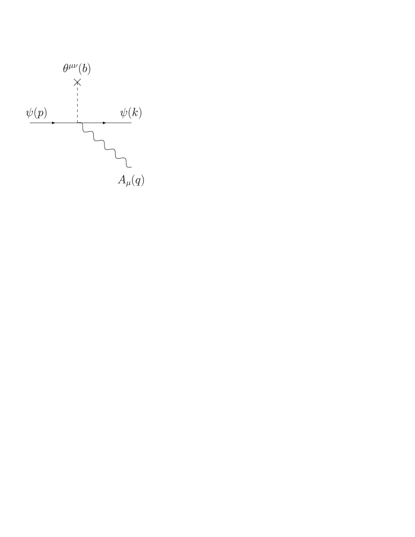
Figure 1: Correction to the two-fermion gauge boson vertex.

It is clear than the dominant signal is a violation of the energy-momentum conservation, as some energy can be absorbed in the background field or released from the background field. Similar effects will occur for the three-gauge-boson interaction and for the two-fermion two-gauge-boson interaction.

4 Models for $\theta(x)$

The function $\theta(x)$ is basically unknown. It depends on the details of the fundamental theory which is at the origin of the non-commutative nature of space-time. Recently non-commutative theories with a non-constant non-commutative parameter have been found in the framework of string theory [35, 36, 37, 38]. But, since we do not know what will eventually turn out to be the fundamental theory at the origin of space-time non-commutativity, we can consider different models for $\theta(x)$. One particularly interesting example for $\tilde{\theta}(b)$, is a Heaviside step function times a constant antisymmetric tensor $\tilde{\theta}^{\mu\nu}(b)=\theta(b_{0}-\Lambda_{R})\theta^{\mu\nu}$. The main motivation for such an ansatz is the as mentioned in [15], the non-commutative nature of space-time sets in only at short distances. A Heaviside function simply implies that there is an energy threshold for the effects of space-time non-commutativity. In that case the vertex studied in (123) becomes

$$\delta^{4}(b_{\mu}-q_{\mu}-k_{\mu}+p_{\mu})\theta(b_{0}-\Lambda_{R})\times$$ (124)

$$\Bigg{(}\frac{i}{2}\theta^{\mu\nu}\bigg{(}p_{\nu}(\mathchoice{\ooalign{$\hfil\displaystyle\mkern 0.0mu/\hfil$\crcr$\displaystyle k$}}{\ooalign{$\hfil\textstyle\mkern 0.0mu/\hfil$\crcr$\textstyle k$}}{\ooalign{$\hfil\scriptstyle\mkern 0.0mu/\hfil$\crcr$\scriptstyle k$}}{\ooalign{$\hfil\scriptscriptstyle\mkern 0.0mu/\hfil$\crcr$\scriptscriptstyle k$}}-m)-k_{\nu}(\mathchoice{\ooalign{$\hfil\displaystyle\mkern 0.0mu/\hfil$\crcr$\displaystyle p$}}{\ooalign{$\hfil\textstyle\mkern 0.0mu/\hfil$\crcr$\textstyle p$}}{\ooalign{$\hfil\scriptstyle\mkern 0.0mu/\hfil$\crcr$\scriptstyle p$}}{\ooalign{$\hfil\scriptscriptstyle\mkern 0.0mu/\hfil$\crcr$\scriptscriptstyle p$}}-m)\bigg{)}-\frac{i}{2}k_{\alpha}\theta^{\alpha\beta}p_{\beta}\gamma^{\mu}\Bigg{)},$$ (141)

where $\theta(b_{0}-\Lambda_{R})$ is the Heaviside step function. In other words, the energy of the decaying particle has to be above the energy $\Lambda_{R}$ corresponding to the distance $R$. Note that we now have two scales, the non-commutative scale $\Lambda_{NC}$ included in $\theta$ and the scale corresponding to the distance where the effects of non-commutative physics set in $\Lambda_{R}$. A small scale of e.g. 1 GeV for $\Lambda_{R}$ is sufficient to get rid of all the constraints coming from low energy experiments and in particular from experiment that are searching for violations of Lorentz invariance. This implies that heavy particles are more sensitive to the non-commutative nature of space-time than the light ones. It would be very interesting to search for a violation of energy conservation in the top quark decays since they are the heaviest particles currently accessible.

Clearly, there are certainly models that are more appropriate than a Heaviside step function. This issue is related to model building and is beyond the scope of the present paper. Our aim was to give a simple example of the type of model that can help to loosen the experimental constraints.

Another interesting possibility is that $\theta^{\mu\nu}$ transforms as a Lorentz tensor: $\theta^{\mu\nu}(x^{\prime})=\Lambda^{\mu}_{\rho}\Lambda^{\nu}_{\sigma}\theta^{\rho\sigma}(x)$ in which case the action we have obtained is Lorentz invariant. It is nevertheless not clear which symmetry acting on $\theta(\hat{x})$, i.e. at the non-commutative level, could reproduce the usual Lorentz symmetry once the expansion in $\theta$ is performed. There are nevertheless examples of quantum groups, where a deformed Lorentz invariance can be defined [39, 40]. Note that if $\theta(x)$ develops a vacuum expectation value, Lorentz invariance is spontaneously broken.

5 Conclusions

We have proposed a formulation of Yang-Mills field theory on a non-commutative space-time described by a space-time dependent anti-symmetric tensor $\theta(x)$. Our results are only valid in the leading order of the expansion in $\theta$. It is nevertheless not obvious that these results can easily be generalized. The basic assumption is that $\theta(x)$ fulfills the Jacobi identity, this insures that the star product is associative.

We have generalized the method developed by Wess and his collaborators to the case of a non-constant field $\theta$, we have derived the Seiberg-Witten maps for the gauge transformations, the gauge fields and the matter fields. The main difficulty is to find the relation between the gauge potential of the covariant coordinates and the Yang-Mills gauge potential.

As expected new operators with derivative acting on $\theta$ are generated in the leading order of the expansion in $\theta$. But, most of them drop out of the action because they correspond to total derivatives.

The main difference between the constant $\theta$ case is that the energy-momentum at each vertex is not conserved from the particles point of view, i.e. some energy can be absorbed or created by the background field. One can consider different models for the deformation $\theta$. It is interesting to note that already a simple model can help to avoid low energy physics constraints. This implies that non-commutative physics becomes relevant again as a candidate for new physics beyond the standard model in the TeV region.

References

• [1] Letter of Heisenberg to Peierls (1930), Wolfgang Pauli, Scientific Correspondence, Vol. II, p.15, Ed. Karl von Meyenn, Springer-Verlag, 1985.
• [2] Letter of Pauli to Oppenheimer (1946), Wolfgang Pauli, Scientific Correspondence, Vol. III, p.380, Ed. Karl von Meyenn, Springer-Verlag, 1993.
• [3] H. S. Snyder, Phys. Rev.  71 (1947) 38.
• [4] J. Wess, “Nonabelian Gauge Theories on Noncommutative Spaces”, talk given at 10th International Conference on Supersymmetry and Unification of Fundamental Interactions (SUSY02), Hamburg, Germany, 17-23 Jun 2002.
• [5] V. Schomerus, JHEP 9906, 030 (1999) [arXiv:hep-th/9903205].
• [6] L. J. Garay, Int. J. Mod. Phys. A 10, 145 (1995) [arXiv:gr-qc/9403008].
• [7] M. Wohlgenannt, arXiv:hep-th/0302070, Plenary talk at XIV International Hutsulian Workshop, Chernivtsi (Ukraine), Oct 28 - Nov 2, 2002.
• [8] J. E. Moyal, Proc. Cambridge Phil. Soc.  45, 99 (1949).
• [9] M. R. Douglas and N. A. Nekrasov, Rev. Mod. Phys.  73, 977 (2001) [arXiv:hep-th/0106048].
• [10] M. Hayakawa, Phys. Lett. B 478, 394 (2000) [arXiv:hep-th/9912094].
• [11] M. Hayakawa, arXiv:hep-th/9912167.
• [12] J. Madore, S. Schraml, P. Schupp and J. Wess, Eur. Phys. J. C 16, 161 (2000) [arXiv:hep-th/0001203].
• [13] B. Jurco, S. Schraml, P. Schupp and J. Wess, Eur. Phys. J. C 17, 521 (2000) [arXiv:hep-th/0006246].
• [14] B. Jurco, L. Moller, S. Schraml, P. Schupp and J. Wess, Eur. Phys. J. C 21, 383 (2001) [arXiv:hep-th/0104153].
• [15] X. Calmet, B. Jurco, P. Schupp, J. Wess and M. Wohlgenannt, Eur. Phys. J. C 23, 363 (2002) [arXiv:hep-ph/0111115].
• [16] A. Bichl, J. Grimstrup, H. Grosse, L. Popp, M. Schweda and R. Wulkenhaar, JHEP 0106, 013 (2001) [arXiv:hep-th/0104097].
• [17] A. A. Bichl, J. M. Grimstrup, L. Popp, M. Schweda and R. Wulkenhaar, arXiv:hep-th/0102103.
• [18] N. Seiberg and E. Witten, JHEP 9909, 032 (1999) [arXiv:hep-th/9908142].
• [19] I. Hinchliffe and N. Kersting, arXiv:hep-ph/0205040; I. Hinchliffe and N. Kersting, Phys. Rev. D 64, 116007 (2001) [arXiv:hep-ph/0104137].
• [20] Z. Chang and Z. z. Xing, Phys. Rev. D 66, 056009 (2002) [arXiv:hep-ph/0204255].
• [21] J. L. Hewett, F. J. Petriello and T. G. Rizzo, Phys. Rev. D 64, 075012 (2001) [arXiv:hep-ph/0010354].
• [22] C. E. Carlson, C. D. Carone and R. F. Lebed, Phys. Lett. B 518, 201 (2001) [arXiv:hep-ph/0107291].
• [23] I. Mocioiu, M. Pospelov and R. Roiban, Phys. Lett. B 489, 390 (2000) [arXiv:hep-ph/0005191]; A. Anisimov, T. Banks, M. Dine and M. Graesser, Phys. Rev. D 65, 085032 (2002) [arXiv:hep-ph/0106356].
• [24] C. P. Martin, Nucl. Phys. B 652, 72 (2003) [arXiv:hep-th/0211164].
• [25] S. M. Carroll, J. A. Harvey, V. A. Kostelecky, C. D. Lane and T. Okamoto, Phys. Rev. Lett.  87, 141601 (2001) [arXiv:hep-th/0105082].
• [26] C. E. Carlson, C. D. Carone and N. Zobin, Phys. Rev. D 66, 075001 (2002) [arXiv:hep-th/0206035].
• [27] K. Morita, Prog. Theor. Phys.  108, 1099 (2003) [arXiv:hep-th/0209234].
• [28] H. Kase, K. Morita, Y. Okumura and E. Umezawa, Prog. Theor. Phys.  109, 663 (2003) [arXiv:hep-th/0212176].
• [29] M. Kontsevich, arXiv:q-alg/9709040.
• [30] A. S. Cattaneo and G. Felder, Commun. Math. Phys.  212, 591 (2000) [arXiv:math.qa/9902090].
• [31] B. Jurco, P. Schupp and J. Wess, Nucl. Phys. B 584, 784 (2000) [arXiv:hep-th/0005005]; see also B. L. Cerchiai, arXiv:hep-th/0304030.
• [32] V. Kathotia, “Kontsevich’s universal formula for deformation quantization and the Campbell-Baker-Hausdorff formula, I,” arXiv:math.QA/9811174.
• [33] G. Dito, Lett. Math. Phys. 48, 307 (1999), [arXiv:math.QA/9905080].
• [34] C. N. Yang and R. L. Mills, Phys. Rev.  96, 191 (1954).
• [35] L. Cornalba and R. Schiappa, Commun. Math. Phys.  225, 33 (2002) [arXiv:hep-th/0101219].
• [36] A. Hashimoto and S. Sethi, Phys. Rev. Lett.  89, 261601 (2002) [arXiv:hep-th/0208126].
• [37] L. Dolan and C. R. Nappi, Phys. Lett. B 551, 369 (2003) [arXiv:hep-th/0210030].
• [38] D. A. Lowe, H. Nastase and S. Ramgoolam, arXiv:hep-th/0303173.
• [39] J. Lukierski, H. Ruegg, A. Nowicki and V. N. Tolstoi, Phys. Lett. B 264, 331 (1991).
• [40] S. Majid and H. Ruegg, Phys. Lett. B 334, 348 (1994) [arXiv:hep-th/9405107].
• [41] H. Weyl, Z. Phys.  46, 1 (1927).