Meson masses in large $N_{f}$ QCD
from the Bethe-Salpeter equation

Abstract

We solve the homogeneous Bethe-Salpeter (HBS) equation for the scalar, pseudoscalar, vector, and axial-vector bound states of quark and anti-quark in large $N_{f}$ QCD with the improved ladder approximation in the Landau gauge. The quark mass function in the HBS equation is obtained from the Schwinger-Dyson (SD) equation in the same approximation for consistency with the chiral symmetry. Amazingly, due to the fact that the two-loop running coupling of large $N_{f}$ QCD is explicitly written in terms of an analytic function, large $N_{f}$ QCD turns out to be the first example in which the SD equation can be solved in the complex plane and hence the HBS equation directly in the time-like region. We find that approaching the chiral phase transition point from the broken phase, the scalar, vector, and axial-vector meson masses vanish to zero with the same scaling behavior, all degenerate with the massless pseudoscalar meson. This may suggest a new type of manifestation of the chiral symmetry restoration in large $N_{f}$ QCD.

1 Introduction

Spontaneous chiral symmetry breaking is one of the most important properties to understand the low-energy phenomena of QCD in the real world. This chiral symmetry is expected to be restored in QCD at several extreme conditions such as QCD with a large number of massless quarks, large $N_{f}$ QCD (see, e.g., Refs. [1, 2, 3, 4, 5, 6, 7]) and QCD in hot and/or dense matter (see, e.g., Ref. [8]). In Ref. [2], based on the infrared (IR) fixed point existing at a two-loop beta function for a large number of massless quarks ($N_{f}\mathrel{\mathchoice{\lower 3.0pt\vbox{\halign{$\m@th\displaystyle\hfill#\hfil$\cr<\crcr\sim\crcr}}}{\lower 3.0pt\vbox{\halign{$\m@th\textstyle\hfill#\hfil$\cr<\crcr\sim\crcr}}}{\lower 3.0pt\vbox{\halign{$\m@th\scriptstyle\hfill#\hfil$\cr<\crcr\sim\crcr}}}{\lower 3.0pt\vbox{\halign{$\m@th\scriptscriptstyle\hfill#\hfil$\cr<\crcr\sim\crcr}}}}\frac{11}{2}N_{c}$) [1], it was found through the improved ladder Schwinger-Dyson (SD) equation that chiral symmetry restoration takes place for $N_{f}$ such that $N_{f}^{\rm crit}<N_{f}<\frac{11}{2}N_{c}$, where $N_{f}^{\rm crit}\simeq 4N_{c}$($=12$ for $N_{c}=3$). Then, in Ref. [3] this chiral restoration at $N_{f}^{\rm crit}$ was further identified with “conformal phase transition” which was characterized by the essential singularity scaling. Moreover, such chiral restoration is also observed by other various methods such as lattice simulation [5], dispersion relation [6], instanton calculus [7], effective field theoretical approach [9], etc..

More attention has been paid to the property of the phase transition. Especially, it is interesting to ask what are the light degrees of freedom near the phase transition point in the large $N_{f}$ QCD: For example, in the manifestation of the chiral symmetry restoration á la the linear sigma model, the scalar bound state becomes a chiral partner of the pseudoscalar bound state and becomes massless at the phase transition point. On the contrary, in the vector manifestation (VM) [10, 11] obtained by the effective field theoretical approach based on the hidden local symmetry model [12], it is the vector bound state which becomes massless as a chiral partner of the pseudoscalar bound state. Besides, from the viewpoint of the conformal phase transition [3], it is natural to suppose that all the existing bound states become massless near the phase transition point when approached from the broken phase (see Ref. [13]).

Then, it is quite interesting to study which types of the bound states actually exist near the phase transition point, and investigate the critical behavior of their masses directly from QCD. Such studies from the first principle will give us a clue to understand the nature of the chiral phase transition in large $N_{f}$ QCD.

A powerful tool to study the bound states of quark and anti-quark directly from QCD is the homogeneous Bethe-Salpeter (HBS) equation in the (improved) ladder approximation (see, for reviews, Refs. [14, 15, 16]). When the mass of the quark is regarded as a constant, we can easily solve the HBS equation by using a so-called fictitious eigenvalue method [14]. However, for consistency with the chiral symmetry, the quark propagator in the HBS equation must be obtained by solving the SD equation with the same kernel as that used in the HBS equation [17, 18, 19, 20], and as a result, the quark mass becomes a certain momentum dependent function. Then, in order to obtain the masses and the wave functions of the bound states, it is necessary to solve the HBS equation and the SD equation simultaneously.

When we try to solve these two equations in real-life ($N_{f}=3$) QCD, however, we encounter difficulties. First of all, for the consistency of the solution of the SD equation with QCD in a high energy region, we need to use the running coupling which obeys the evolution determined from QCD $\beta$-function in the high energy region (see, for reviews, Refs. [15, 16]). Since the running coupling diverges at some infrared scale, $\Lambda_{\rm QCD}$, we have to regularize the running coupling in the low energy region, for which there exist several ways (see, e.g., Refs. [21, 22, 23, 24, 25]). Even if we fix the infrared regularization in such a way that we can solve the SD equation on the real (space-like) axis, another problem arises when we try to solve the HBS equation. Since the argument of the quark mass function in the HBS equations for the massive bound states becomes a complex quantity after the Wick rotation has been made, we have to solve the SD equation on the complex plane, which requires an analytic continuation of the running coupling. Several works such as in Refs. [26, 27] proposed models of running couplings for a general complex variable which are consistent with perturbative QCD for large space-like momentum. However, they still have branch cuts on the complex plane, and it is a complicated task to obtain the solution of the SD equation for a general complex variable. One way to avoide a such complication is solving the inhomogeneous BS equation for vertex functions to obtain the current correlators in the space-like region which we can fit the mass of the relevant bound state to (see, e.g., Refs. [28, 29]). Another way might be replacing the entire running coupling with an ad hoc analytic function (see, e.g., Ref. [30]). Anyway, it is impossible to solve the SD equation on the complex plane without modeling the running coupling.

In this paper, we point out that the situation dramatically changes when we increase the number of massless quarks. When $N_{f}$ becomes larger than $\ N_{f}^{\ast}\simeq 8.05$, the running coupling obtained from the renormalization group equation (RGE) with two-loop approximation takes a finite value for all the range of the energy region due to the emergence of the non-trivial IR fixed point. Then, we need no infrared regularization, and we do not have any ambiguities coming from the regularization scheme which do exist in the case of small $N_{f}$. Moreover, an explicit solution of the two-loop RGE can be written in terms of the Lambert $W$ function [4, 31], and when $N_{f}$ is close to $N_{f}^{\rm crit}$ the solution of the RGE has no singularity on the complex plane except for the time-like axis [31]. Consequently, we can solve the SD equation on the complex plane without introducing any models for the running coupling.

Based on these facts, we solve the HBS equations for the bound states of quark and anti-quark in large $N_{f}$ QCD with the improved ladder approximation in the Landau gauge. The mass function for complex arguments needed in the HBS equation is obtained by solving the SD equation with the same kernel as that used in the HBS equation. We find the solution of the HBS equation in each of the scalar, vector, and axial-vector channels, which implies that the scalar, vector, and axial-vector bound states are actually formed near the phase transition point. Our results show that the masses of the scalar, vector, and axial-vector bound states go to zero as the number of quarks $N_{f}$ approaches to its critical value $N_{f}^{\rm crit}$ where the chiral symmetry restoration takes place. This may suggest the existence of a new type of manifestation of chiral symmetry restoration in large $N_{f}$ QCD other than the linear sigma model like manifestation and a simple version of the vector manifestation proposed in Ref. [10].

This paper is organized as follows. In section 2 we numerically solve the SD equation with an approximate form of the running coupling, and study the critical behavior of the Nambu-Goldstone boson decay constant. In section 3 we solve the SD equation for complex arguments. Section 4 is devoted to summarizing the numerical method for solving the HBS equation. Section 5 is the main part of this paper. We first solve the HBS equation for the pseudoscalar bound state to show that the approximation adopted in the present analysis is consistent with the chiral symmetry. We next solve the HBS equation for the scalar, vector, and axial-vector bound states to obtain their masses. Finally we give a summary and discussion in section 6. In Appendix A we solve the HBS equation for the ortho-positronium with a constant electron mass to show the validity of the fictitious eigenvalue method. The bispinor bases for the bound states are listed in Appendix B. In Appendix C we calculate the coupling constants $F_{V}$, $F_{A}$, and $G_{S}$ of the vector, axial-vector, and scalar bound states to the vector current, axial-vector current, and scalar density. We briefly study numerical uncertainties in the present analysis in Appendix D.

2 Schwinger-Dyson equation in large $N_{f}$ QCD

In this section we numerically solve the Schwinger-Dyson (SD) equation for the quark propagator with the improved ladder approximation in the Landau gauge, and show the critical behaviors of the dynamical mass and the decay constant of the Nambu-Goldstone boson. We also show the behavior of the fermion-antifermion pair condensate $\ \langle\bar{\psi}\psi\rangle\$ near the phase transition point.

2.1 SD equation in the (improved) ladder approximation

Schwinger-Dyson (SD) equation is a powerful tool to study the dynamical generation of the fermion mass directly from QCD (for reviews, see, e.g., Refs. [15, 16]). The SD equation for the full fermion propagator $\ iS_{F}^{-1}=A(p^{2})\hbox to0.0pt{\hbox to5.03125pt{\hfil/\hfil}\hss}p-B(p^{2})\$ in the improved ladder approximation [22, 21] is given by (see Fig. 1 for a graphical expression)

$$iS_{F}^{-1}(p)-\hbox to0.0pt{\hbox to5.03125pt{\hfil/\hfil}\hss}p\ =\ C_{2}\int\frac{d^{4}q}{i(2\pi)^{4}}\ \bar{g}^{2}(p,q)\ \frac{1}{(p-q)^{2}}\left(g_{\mu\nu}-\frac{(p-q)_{\mu}(p-q)_{\nu}}{(p-q)^{2}}\right)\gamma^{\mu}\ iS_{F}(q)\ \gamma^{\nu},$$ (2.1)

where $\ C_{2}\left(=\frac{N^{2}_{c}-1}{2N_{c}}\right)\$ is the second casimir invariant, and $\ \bar{g}(p,q)\$ is the running coupling. The Landau gauge is adopted for the gauge boson propagator.

Figure 1: A graphical expression of the SD equation in the (improved) ladder approximation.

The SD equation provides coupled equations for two functions $A$ and $B$ in the full fermion propagator $S_{F}$. When we use a simple ansatz for the running coupling, $\bar{g}^{2}(p,q)=\bar{g}^{2}(\max(p_{E}^{2},q_{E}^{2}))$ [22, 21], with $(p_{E}^{2},q_{E}^{2})$ being the Euclidean momenta, we can carry out the angular integration and get $A(p^{2})\equiv 1$ in the Landau gauge. Then the SD equation becomes a self-consistent equation for the mass function $\Sigma(p^{2})\equiv B(p^{2})$. The resultant asymptotic behavior of the dynamical mass $\Sigma(p^{2})$ is shown to coincide with that obtained by the operator product expansion technique [15, 16].

However, it was shown in Ref. [18] that the axial Ward-Takahashi identity is violated in the improved ladder approximation unless the gluon momentum is used as the argument of the running coupling as $\bar{g}^{2}((p_{E}-q_{E})^{2})$. In this choice we cannot carry out the angle integration analytically since the running coupling depends on the angle factor $\cos{\theta}=p_{E}\cdot q_{E}/|p_{E}||q_{E}|$. Furthermore, we would need to introduce a nonlocal gauge fixing [18] to preserve the condition $A=1$.

In Ref. [24], however, it was shown that an angle averaged form $\bar{g}^{2}(p_{E}^{2}+q_{E}^{2})$ gives a good approximation. Then, in the present analysis we take the argument of the running coupling as

$$\bar{g}^{2}(p_{E},q_{E})\ \Rightarrow\ \bar{g}^{2}(p_{E}^{2}+q_{E}^{2}).$$ (2.2)

After applying this angle approximation and carrying out the angular integration, we can show (see, e.g., Refs. [32, 33, 15, 16]) that $A$ always satisfies $A(p^{2})=1$ in the Landau gauge. Then the SD equation becomes

$$\Sigma(x)=C_{2}\ \frac{3}{16\pi^{2}}\int dy\ \frac{y\ \Sigma(y)}{y+\Sigma^{2}(y)}\ \frac{\bar{g}^{2}(x+y)}{\max(x,y)}\ ,$$ (2.3)

where $\ x=p_{E}^{2}\$ and $\ y=q_{E}^{2}\$. Although the choice of arguments in Eq. (2.2) explicitly breaks the chiral symmetry as mentioned above, it will be shown later that the magnitude of the breaking is negligible.

2.2 Running coupling in large $N_{f}$ QCD

In QCD with $N_{f}$ flavors of massless quarks, the renormalization group equation (RGE) for the running coupling $\alpha(\mu)\ \Big{(}=\frac{\bar{g}^{2}(\mu)}{4\pi}\,\Big{)}$ in the two-loop approximation is given by

$$\mu\frac{d}{d\mu}\alpha(\mu)=-b\alpha^{2}(\mu)-c\alpha^{3}(\mu),$$ (2.4)

where

$$b=\frac{1}{6\pi}\left(11N_{c}-2N_{f}\right)\ ,\quad c=\frac{1}{24\pi^{2}}\left(34N_{c}^{2}-10N_{c}N_{f}-3\frac{N_{c}^{2}-1}{N_{c}}N_{f}\right)\ .$$ (2.5)

From the above beta function we can easily see that, when $b>0$ and $c<0$, i.e., $N_{f}$ takes a value in the range of $N_{f}^{*}<N_{f}<\frac{11}{2}N_{c}$ ($N_{f}^{\ast}\simeq 8.05$ for $N_{c}=3$), the theory is asymptotically free and the beta function has a zero, corresponding to an infrared stable fixed point [1, 2], at

$$\alpha_{\ast}=-\ \frac{\ b\ }{\ c\ }\ .$$ (2.6)

Existence of the infrared fixed point implies that the running coupling takes a finite value even in the low energy region. Actually, the solution of the two loop RGE in Eq. (2.4) can be explicitly written [31, 34] in all the energy region as

$$\alpha(\mu)=\alpha_{\ast}\left[\ W(\mu^{\,b\alpha_{\ast}}/e\Lambda^{b\alpha_{\ast}})+1\ \right]^{-1},$$ (2.7)

where $W(x)=F^{-1}(x)$ with $F(x)=xe^{x}$ is the Lambert $W$ function, and $\Lambda$ is a renormalization group invariant scale defined by [2]

$$\Lambda\ \equiv\ \mu\ \exp\left[-\frac{1}{b\ \alpha_{\ast}}\log\left(\frac{\alpha_{\ast}-\alpha(\mu)}{\alpha(\mu)}\right)-\frac{1}{b\ \alpha(\mu)}\right].$$ (2.8)

We note that, in the present analysis, we fix the value of $\Lambda$ to compare the theories with a different number of flavors, and that we have no adjustable parameters in the running coupling in Eq. (2.7), accordingly (see discussion below). We show an example of $\alpha(\mu)$ for $N_{f}=9$ by the solid line in Fig. 2.

Figure 2: Two-loop running coupling (solid line) compared with the approximate form in Eq. (2.9) (dashed line) for $N_{f}=9$.

The fact that the running coupling is expressed by a certain function as in Eq. (2.7) implies that, in the case of large $N_{f}$ QCD, we do not need to introduce any infrared regularizations such as the ones adopted in Refs. [21, 22, 23] for studying real-life QCD with small $N_{f}$ in which the infrared regularization parameter must be chosen in such a way that the running coupling in the infrared region becomes larger than the critical value $\alpha_{\rm cr}=\pi/4$ for realizing the dynamical chiral symmetry breaking [21]. The running coupling in large $N_{f}$ QCD takes a certain value in the infrared region for given $N_{f}$, so that we can definitely determine, within the framework of the SD equation, whether or not the dynamical chiral symmetry breaking is realized. Actually, the value of $\alpha_{\ast}$ decreases monotonically with increasing $N_{f}$, and the chiral symmetry restores when $N_{f}$ becomes large enough. In Refs. [2, 4], it was shown that the phase transition occurs at $N_{f}^{\rm crit}\simeq 11.9$ for $N_{c}=3$ (corresponding to $\alpha_{\ast}=\alpha_{\rm cr}=\pi/4$).

In order to reduce the task of numerical calculations in solving the HBS equation, we modify the shape of the running coupling. Since the dynamics in the infrared region governs the chiral symmetry breaking, we adopt the following approximation for the running coupling  [3, 4]:

$$\frac{\bar{g}^{2}(x+y)}{4\pi}=\alpha_{\ast}\ \theta(\Lambda^{2}-(x+y))\ .$$ (2.9)

In this approximation the coupling takes the constant value $\alpha_{\ast}$ (the value at the IR fixed point) below the scale $\Lambda$ and entirely vanishes in the energy region above this scale. The dashed line In Fig. 2 represents the approximated form of the running coupling for $N_{f}=9$.

2.3 Numerical solution for the SD equation

In this subsection we briefly explain how we solve the SD equation numerically.

We first introduce the infrared (IR) cutoff $\lambda_{SD}$ and ultraviolet (UV) cutoff $\Lambda_{SD}$ as

$$\Lambda^{2}\ e^{\lambda_{SD}/\Lambda}\ \leq\ x\,,\ y\ \leq\ \Lambda^{2}\ e^{\Lambda_{SD}/\Lambda}\ .$$ (2.10)

Then, we discretize the momentum variable $x$ and $y$ into $N_{SD}$ points as

$$x_{i}=\Lambda^{2}\ \exp\Big{[}\lambda_{SD}/\Lambda+D_{SD}\cdot i\,\Big{]}\ ,\ \ \ \Big{(}i=0,1,2,\cdots,(N_{SD}-1)\Big{)}\ ,$$ (2.11)

where

$$D_{SD}=\frac{\ (\Lambda_{SD}-\lambda_{SD})/\Lambda\ }{N_{SD}-1}\ .$$ (2.12)

Accordingly, the integration over $y$ is replaced with a summation as

$$\int dy\ \Rightarrow\ D_{SD}\sum_{j}y_{j}\ .$$ (2.13)

Then, the SD equation in Eq. (2.3) with the running coupling in Eq. (2.9) is rewritten as

$$\Sigma(x_{i})\ =\ \frac{1}{4\pi^{2}}\ D_{SD}\sum_{j}\ \bar{g}^{2}(x_{i}+y_{j})\ \frac{y_{j}^{2}}{\max(x_{i},\ y_{j})}\ \frac{\Sigma(y_{j})}{y_{j}+\Sigma^{2}(y_{j})}.$$ (2.14)

This discretized version of the SD equation is solved by the recursion relation:

$$\Sigma_{(n+1)}(x_{i})=\frac{1}{4\pi^{2}}D_{SD}\sum_{j}\bar{g}^{2}(x_{i}+y_{j})\ \frac{y_{j}^{2}}{\max(x_{i},\ y_{j})}\ \frac{\Sigma_{(n)}(y_{j})}{y_{j}+\Sigma_{(n)}^{2}(y_{j})}\ .$$ (2.15)

Starting from a suitable initial condition (we choose $\Sigma_{(0)}(x_{i})=1$), we update the mass function by the above recursion relation. Then, we stop the iteration when the convergence condition

$$D_{SD}\sum_{i}\frac{x^{2}_{i}}{16\pi^{2}}\,\Big{[}\,\Sigma_{(n+1)}(x_{i})-\Sigma_{(n)}(x_{i})\,\Big{]}^{2}\ <\ \varepsilon^{2}\Lambda^{6}$$ (2.16)

is satisfied for sufficiently small $\varepsilon$, and regard this $\Sigma_{(n)}$ as a solution of Eq. (2.14). In Fig. 3, we show the numerical solution for the mass function $\Sigma(x)$.

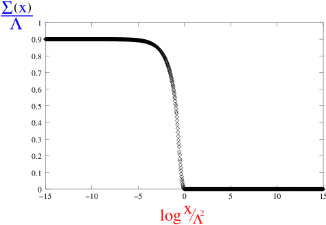
Figure 3: A solution of the discretized SD equation in Eq. (2.14) for $N_{f}=9$.

Here, we took $N_{f}=9\$ ($\alpha_{\ast}\simeq 5.2$) as an example and used the following parameters:

$$\Lambda_{SD}/\Lambda=+15\ \ ,\ \ \lambda_{SD}/\Lambda=-15\ \ ,\ \ N_{SD}=1000\ \ ,\ \ \varepsilon=10^{-15}.$$ (2.17)

Now, let us study the critical behavior of the fermion mass as $N_{f}$ is varied. Note that we can use $\alpha_{\ast}$ instead of $N_{f}$ as an input parameter, because once we choose a value of $N_{f}$, the value of $\alpha_{\ast}$ is uniquely determined from Eq. (2.6). For example, $\alpha_{\ast}=1$ implies $N_{f}=11.42$ and $\alpha_{\ast}=\alpha_{\rm cr}$ implies $N_{f}=11.91$. We solve Eq. (2.14) for various values of $\alpha_{\ast}$ and plot the values of $\ \Sigma(m^{2})\$ in Fig. 4.

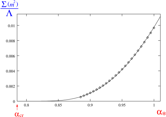
Figure 4: Numerical solutions of $\Sigma(x=m^{2})$ for several values of $\alpha_{\ast}$ (indicated by $\Diamond$). Solid line shows the function in Eq. (2.19) with the best fitted value $d=4.0$.

Here, $\ m\$ represents the dynamical mass defied by $\ m=\Sigma(m^{2})\$. It should be noticed that $m$ is defined in the space-like region which does not represent the pole mass of fermion. As we will show in section 3, the present fermion propagator does not have any poles and then there are no pole masses of fermion.

We compare this result with the analytic solution [3, 4]:

$$\Sigma(m^{2}) \approx \Lambda\ \exp\left(-\frac{\pi}{\sqrt{\frac{\alpha\ast}{\alpha_{\rm cr}}-1\ }}\right)\hskip 32.43611pt\mbox{for}\ \ \alpha_{\ast}>\alpha_{\rm cr}\ .$$ (2.18)

In the above form there is an ambiguity in the prefactor. Then, we introduce the function

$$h(\alpha_{\ast})=d\,\Lambda\,\exp\left(-\frac{\pi}{\sqrt{\frac{\alpha\ast}{\alpha_{\rm cr}}-1\ }}\right)\ ,$$ (2.19)

and fit the value of the pre-factor $d$ by minimizing

$$\sum_{\alpha_{\ast}}\left|\,\Sigma(x=m^{2};\alpha_{\ast})-h(\alpha_{\ast})\,\right|^{2}\ ,$$ (2.20)

in the range of $\alpha_{\ast}\in[0.885:1]$. The resultant best fitted value of $d$ is

$$d\simeq 4.0\ .$$ (2.21)

We plot the function in Eq. (2.19) with the best fitted value $d=4.0$ in Fig. 4 (solid line). This clearly shows that the $\alpha_{\ast}$-dependence of the resultant $\Sigma(m^{2})$ from our numerical calculation is consistent with the analytic result: The dynamical mass function vanishes when $\alpha_{\ast}$ reaches the critical value $\alpha_{\rm cr}=\pi/4$. Noting that decreasing $\alpha_{\ast}$ corresponds to increasing $N_{f}$ for fixed $N_{c}$ as we discussed in the previous subsection, we see that the chiral symmetry restoration actually occurs at $N_{f}=N_{f}^{\rm crit}\simeq 12\,(N_{c}/3)$ [2, 4].

2.4 Pseudoscalar meson decay constant in large $N_{f}$ QCD

So far we have solved the SD equation and obtained the mass functions for the various values of $\alpha_{\ast}$. Now we can calculate the pseudoscalar meson decay constant $F_{P}$ at each $\alpha_{\ast}$ by using the Pagels-Stokar formula [35]:

$$F_{P}^{2}\ =\ \frac{N_{c}}{4\pi^{2}}\int dx\ \frac{\ x\ \Sigma^{2}(x)\ -\ \frac{\ x^{2}}{4}\ \frac{d}{dx}\left[\ \Sigma^{2}(x)\ \right]\ }{\left(\ x\ +\ \Sigma^{2}(x)\ \right)^{2}}.$$ (2.22)

In Fig. 5, we plot the values of $F_{P}$ for several values of $\alpha_{\ast}$ (indicated by $\Diamond$). To study the critical behavior of the pseudoscalar meson decay constant we use the function of the form in Eq. (2.19) and fit the value of $d$ by minimizing

$$\sum_{\alpha_{\ast}}\left|F_{P}(\alpha_{\ast})-h(\alpha_{\ast})\right|^{2}\ ,$$ (2.23)

for $\alpha_{\ast}\in[0.885:1]$. The resultant best fitted value of $d$ is

$$d\simeq 1.5\ (\equiv d_{F_{P}})\ .$$ (2.24)

We plot the fitting function with $d=1.5$ in Fig. 5 (dotted line). This shows that the results of the numerical calculations for $F_{P}$ are well fitted by the function of the form in Eq. (2.19), and that the pseudoscalar meson decay constant has the same critical behavior as the mass function has.

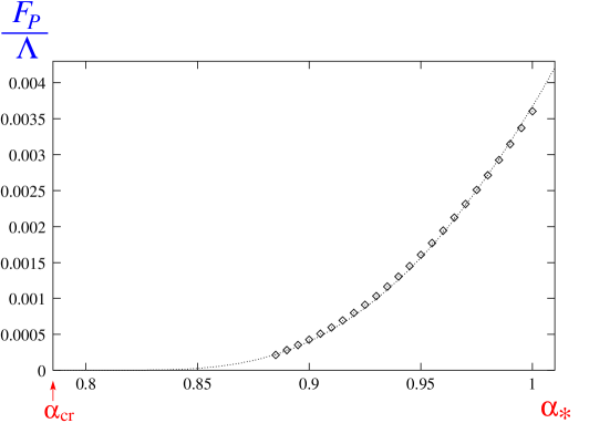
Figure 5: Values of $F_{P}$ calculated from the Pagels-Stokar formula for several values of $\alpha_{\ast}$ (indicated by $\Diamond$). The dotted line shows the function of the form in Eq. (2.19) with the best fitted value $d=1.5$.

2.5 Fermion-antifermion pair condensate

In this subsection, we calculate the fermion-antifermion pair condensate $\langle\bar{\psi}\psi\rangle$ in large $N_{f}$ QCD, and show that the system in the present analysis has the large anomalous dimension $\gamma_{m}$ for the operator $\bar{\psi}\psi$. We also show that the values of $\gamma_{m}$ are not affected so much by the approximation for the running coupling used in the present analysis.

The condensate $\langle\bar{\psi}\psi\rangle$ is calculated from the following equation:

$$\langle\bar{\psi}\psi\rangle_{\Lambda_{UV}}\ =\ -\frac{N_{c}}{4\pi^{2}}\int_{0}^{\Lambda_{UV}^{2}}dx\ \frac{x\ \Sigma(x)}{\ x+\Sigma^{2}(x)\ },$$ (2.25)

where $\Sigma(x)$ is the mass function obtained from the SD equation and $\Lambda_{UV}$ represents UV cutoff introduced to regularize the UV divergence. In the improved ladder approximation, the high-energy behavior of the mass function is consistent with that derived using the operator product expansion (OPE). The chiral condensate calculated using the mass function was shown to obey the renormalization group equation derived with the OPE (see, e.g., Refs. [15, 16]). Then, as was adopted in Refs.[2, 3, 4], we identify the condensate, which is calculated with UV cutoff $\Lambda_{UV}$, with that renormalized at the scale $\Lambda_{UV}$ in QCD.

We expect that infrared dynamics in large $N_{f}$ QCD is similar to that of strong coupling QED or walking gauge theories [36] since the running coupling in large $N_{f}$ QCD is well approximated by the constant coupling (see Fig. 2)  [4]. Then, we also expect that the value of the anomalous dimension in large $N_{f}$ QCD becomes $\gamma_{m}\simeq 1$ since the walking gauge theories have $\gamma_{m}\simeq 1$  [36].

When a considering system has the anomalous dimension $\gamma_{m}$, scaling properties of $F_{P}$ and $-\langle\bar{\psi}\psi\rangle$ with respect to $\alpha_{\ast}$ near the critical point are expressed as follows [36] :

$$F_{P}\sim m,$$ (2.26)

$$-\langle\bar{\psi}\psi\rangle\sim m^{3-\gamma_{m}},$$ (2.27)

where $m$ represents the dynamical fermion mass. These equations mean that the relation between $\langle\bar{\psi}\psi\rangle$ and $F_{P}$ can be written as

$$-\langle\bar{\psi}\psi\rangle=c\cdot F_{P}^{3-\gamma_{m}},$$ (2.28)

where $c$ is a certain positive constant. From this equation, we can express the anomalous dimension as

$$\gamma_{m}\ =\ \gamma^{\prime}_{m}\ -\ \varepsilon,$$ (2.29)

where

$$\gamma^{\prime}_{m} = 3-\frac{\log(-\langle\bar{\psi}\psi\rangle)}{\log F_{P}},$$ (2.30)

$$\varepsilon = \frac{\log c}{-\log F_{P}}.$$ (2.31)

Here, we note that $\gamma^{\prime}_{m}$ approaches $\gamma_{m}$ for $\alpha_{\ast}\rightarrow\alpha_{\rm cr}$ since $F_{P}$ becomes small, i.e., $\ (-\log F_{P})\gg 1$, near the critical point (see Fig. 5):

$$\varepsilon\rightarrow 0\ \ \ \ \ \ \mbox{for}\ \ \alpha_{\ast}\rightarrow\alpha_{\rm cr}.$$ (2.32)

In Fig. 6, we plot the values of $\gamma^{\prime}_{m}$ for several values of $\alpha_{\ast}$ as an estimation of the anomalous dimension.

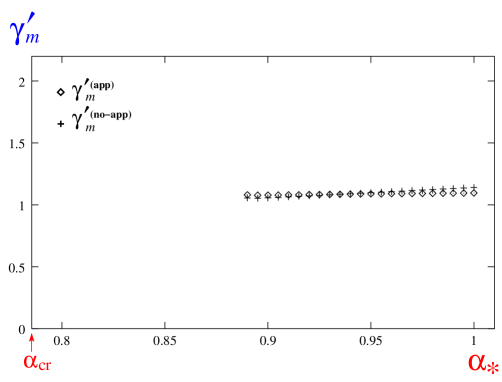
Figure 6: Values of $\gamma^{\prime}_{m}$ for several values of $\alpha_{\ast}$. $\Diamond$ and $+$ represent the values of $\gamma^{\prime}_{m}$ calculated from Eq. (2.30) with and without approximation for the running coupling. (We call them $\ {\gamma^{\prime}}_{m}^{{\bf(app)}}\$ and $\ {\gamma^{\prime}}_{m}^{{\bf(no-app)}}\$ respectively.)

The data indicated by $\Diamond$ in Fig. 6 is obtained with the approximated running coupling (dashed line in Fig. 2) in the SD equation. (We call this kind of data ${\gamma^{\prime}}_{m}^{\bf(app)}$.) On the other hand, the data indicated by $+$ is the result from the calculation with the two-loop running coupling given in Eq. (2.7). (We call this kind of data $\ {\gamma}_{m}^{{\bf(no-app)}}\$.) From these results, we conclude that large $N_{f}$ QCD with two-loop running coupling as well as with approximated running coupling actually possesses

$$\gamma_{m}\simeq\gamma^{\prime}_{m}\simeq 1.$$ (2.33)

Moreover, Fig. 6 shows that the data of $\ {\gamma^{\prime}}_{m}^{{\bf(app)}}\$ is in good agreement with that of $\ {\gamma^{\prime}}_{m}^{{\bf(no-app)}}\$, which implies that the approximation for the running coupling used in the present analysis works well. We also expect that the approximation does not affect the results so much when we calculate the HBS equations for the bound states.

3 SD equation on the complex plane

As we will discuss in section 4, we need the mass function for complex arguments when we solve the HBS equation for the massive bound state. In this section, we first introduce the SD equation for the complex argument following Ref. [37] (see also Ref. [38]), and then solve it in the case of large $N_{f}$ QCD.

The SD equation for the complex argument is expressed as [37]

$$\Sigma(x)=C_{2}\frac{3}{16\pi^{2}}\left[\int_{C(0,x)}dy\frac{y}{x}+\int_{C(x,\infty)}dy\right]\frac{\bar{g}^{2}(x+y)\,\Sigma(y)}{y+{\Sigma^{2}(y)}}\ ,$$ (3.34)

where $C(a,b)$ is the integral path on the complex plane. Here, we took the same argument of the running coupling as that in Eq. (2.2), and carried out the angle integration. Note that the integral path $C(a,b)$ must be taken so as to avoid the branch cut appearing in the integral.

We first study the structure of the running coupling appearing in the SD equation (3.34) to clarify the branch cut. In the improved ladder approximation it is essential to use the running coupling determined from the $\beta$-function in the high energy (space-like) region for consistency with perturbative QCD. In QCD with small $N_{f}$, however, the running coupling obtained from the perturbative $\beta$-function diverges at some infrared scale, $\Lambda_{\rm QCD}$. In the ordinary SD equation in the space-like region, the infrared singularity is avoided by introducing infrared regularization such as the so-called Higashijima-Miransky approximation [21, 22] and its extension as in Ref. [23]. However, since the running coupling in Eq. (3.34) is a complex function which has the complex argument, we need an extension with analyticity satisfied. Several works such as in Refs. [26, 27] proposed models of running coupling which are consistent with perturbative QCD in the high energy region. But they still have branch cuts on the complex plane, and it is a burdensome task to evade all the branch cuts by carefully selecting the integral path in Eq. (3.34). One way to avoide such a complication might be to give up the consistency with perturbative QCD and use models of running coupling with analyticity such as the one used in Ref. [30].

Here we point out that the situation dramatically changes in the large $N_{f}$ QCD. In the case of large $N_{f}$ QCD, as we explained in subsection 2.2, the running coupling, as well as the two-loop $\beta$-function, is finite for any space-like momentum. This implies that we may be able to construct the running coupling by analytic continuation using the $\beta$-function. Actually, an explicit solution of the two-loop renormalization group equation (RGE) can be written in terms of the Lambert $W$ function [4, 31]. When $N_{f}$ is close to $N_{f}^{\rm crit}$, the solution of the RGE has no singularity on the complex plane except for the time-like axis [31].

As a result, for general complex $x$ except on the time-like axis ($x<0$), we can take the integral path $C(a,b)$ in such a way that it just avoids the branch cut coming from the angle integration. In Fig. 7 we show the branch cut together with a simple choice of the integral path [37].

Figure 7: Integral path of the SD equation (3.34). Here, the branch cut appears from the four-dimensional angle integration.

We stress again that the reason why we can take this simple integral path is that the running coupling has no singularity on the complex plane except for the time-like axis.

For solving the SD equation on the complex plane, we here study the explicit form of the running coupling. In Fig. 8 we show the real part of the running coupling on the complex plane which is obtained by performing the analytic continuation from the running coupling on the real axis determined from the two-loop $\beta$-function.

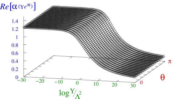
Figure 8: Real part of the two-loop running coupling for $N_{f}=11$ on the complex plane obtained by the analytic continuation from the running coupling on the real axis (we use the Cauchy-Rieman relation). The complex argument of $\alpha$ is expressed as $y=Ye^{i\theta}$, where $Y$ and $\theta$ are real. Note that $y$ is in the space-like region for $\theta=0$ and in the time-like region for $\theta=\pi$.

This figure shows that $\mbox{Re}\alpha\simeq\alpha_{\ast}$, i.e., $\mbox{Im}\alpha\simeq 0$, in the range of $Y=|y|<\Lambda^{2}$, and that $\mbox{Re}\alpha\ll\alpha_{\ast}$ in the range of $Y>\Lambda^{2}$. Thus we take the following approximation for the running coupling on the complex plane:

$$\alpha(y)\ =\ \alpha_{\ast}\ \theta(\Lambda^{2}-Y)\ ,$$ (3.35)

which is smoothly connected to the approximation adopted in Eq. (2.9) for the running coupling on the space-like axis.

Now, let us solve the SD equation (3.34) to obtain the mass function for complex variable $x$. Along the integral path shown in Fig. 7, the variables $x$ and $y$ are parametrized as

$$x=Xe^{i\theta},\ \ y=Ye^{i\theta},$$ (3.36)

where $X$, $Y$, and $\theta$ are real. Then the SD equation (3.34) is rewritten as

$$\Sigma(Xe^{i\theta})=C_{2}\frac{3}{16\pi^{2}}\left[\int_{0}^{X}dY\frac{Y}{X}+\int_{X}^{\infty}dY\right]\frac{\bar{g}^{2}(X+Y)\,\Sigma(Ye^{i\theta})}{Y+e^{-i\theta}\,\Sigma^{2}(Ye^{i\theta})}\ .$$ (3.37)

From this we can easily see that the solution is expressed as

$$\Sigma(x)=e^{i\frac{\theta}{2}}\,\bar{\Sigma}(X)\ ,$$ (3.38)

where $\bar{\Sigma}(X)$ is real and satisfies the original SD equation on the real axis:

$$\bar{\Sigma}(X)=C_{2}\frac{3}{16\pi^{2}}\left[\int_{0}^{X}dY\frac{Y}{X}+\int_{X}^{\infty}dY\right]\frac{\bar{g}^{2}(X+Y)\,\bar{\Sigma}(Y)}{Y+{\bar{\Sigma}(Y)}^{2}}\ .$$ (3.39)

Note that the fermion propagator $S_{F}$ does not have any poles since the kinetic part $x$ and the mass part $\Sigma^{2}(x)$ have the same phases as $x+\Sigma^{2}(x)=e^{i\theta}(X+\bar{\Sigma}^{2}(X))$ [see Eq. (3.38)] and the mass function in the space-like region satisfies $X+\bar{\Sigma}^{2}(X)>0$.

We should note that the above solution in Eq. (3.38) is a double-valued function on the complex plane: The variable $x=Xe^{i\theta}$ can be parametrized as $x=Xe^{i(\theta+2\pi)}$ for which the solution takes $\Sigma(x)=e^{i(\theta/2+\pi)}\bar{\Sigma}(X)=-e^{i\theta/2}\bar{\Sigma}(X)$. This corresponds to the fact that the SD equation has two solutions: When $\Sigma(x)$ is a solution, $-\Sigma(x)$ also satisfies the equation. When we choose the range of $\theta$ as $\theta\in[-\pi:\pi]$, the branch cut emerges on the time-like axis. This choice is natural because the appearance of the branch cut in the time-like region seems consistent with the analytic structure of the running coupling. We will see that this branch cut does not matter in calculating the bound state masses.

4 Homogeneous Bethe-Salpeter equation

In this section we briefly review the homogeneous Bethe-Salpeter (HBS) equation for the bound states of quark and antiquark and show how to solve it numerically.

4.1 Bethe-Salpeter amplitude

In this paper, we consider the scalar, pseudoscalar, vector, and axial-vector bound states of quark and antiquark, and we write these bound states as $|S(q)\rangle$, $|P(q)\rangle$, $|V(q,\epsilon)\rangle$, and $|A(q,\epsilon)\rangle$, respectively. Here, $q^{\mu}$ represents the momentum of the bound states and $\epsilon^{\mu}$ represents the polarization vector satisfying $\epsilon\cdot q=0$ and $\epsilon^{2}=-1$.

Now, we introduce the Bethe-Salpeter (BS) amplitudes $\chi$ for the bound states of quark and anti-quark as follows :

$$\langle 0|\ T\ \psi_{\alpha fi}(x_{+})\ \bar{\psi}_{\beta}^{f^{\prime}j}(x_{-})\ |S_{a}(q)\rangle\ =\ \delta_{i}^{j}\frac{(\lambda_{a})_{f}^{f^{\prime}}}{\sqrt{2}}\,e^{-iqX}\int\frac{d^{4}p}{(2\pi)^{4}}e^{-ipr}[\chi_{(S)}(p;q)]_{\alpha\beta},$$ (4.40)

$$\langle 0|\ T\ \psi_{\alpha fi}(x_{+})\ \bar{\psi}_{\beta}^{f^{\prime}j}(x_{-})\ |P_{a}(q)\rangle\ =\ \delta_{i}^{j}\frac{(\lambda_{a})_{f}^{f^{\prime}}}{\sqrt{2}}\,e^{-iqX}\int\frac{d^{4}p}{(2\pi)^{4}}e^{-ipr}[\chi_{(P)}(p;q)]_{\alpha\beta},$$ (4.41)

$$\langle 0|\ T\ \psi_{\alpha fi}(x_{+})\ \bar{\psi}_{\beta}^{f^{\prime}j}(x_{-})\ |V_{a}(q,\epsilon)\rangle\ =\ \delta_{i}^{j}\frac{(\lambda_{a})_{f}^{f^{\prime}}}{\sqrt{2}}\,e^{-iqX}\int\frac{d^{4}p}{(2\pi)^{4}}e^{-ipr}[\chi_{(V)}(p;q,\epsilon)]_{\alpha\beta},$$ (4.42)

$$\langle 0|\ T\ \psi_{\alpha fi}(x_{+})\ \bar{\psi}_{\beta}^{f^{\prime}j}(x_{-})\ |A_{a}(q,\epsilon)\rangle\ =\ \delta_{i}^{j}\frac{(\lambda_{a})_{f}^{f^{\prime}}}{\sqrt{2}}\,e^{-iqX}\int\frac{d^{4}p}{(2\pi)^{4}}e^{-ipr}[\chi_{(A)}(p;q,\epsilon)]_{\alpha\beta},$$ (4.43)

where $x_{\pm}=X\pm r/2$, $\lambda_{a}$ is the generator of $\mbox{SU}(N_{f})$ normalized as $\mbox{tr}[\lambda_{a}\lambda_{b}]=2\delta_{ab}$, and ($\alpha$, $\beta$), ($f$, $f^{\prime}$), and ($i$, $j$) denote the spinor, flavor, and color indices, respectively.

We can expand the BS amplitude $\chi$ in terms of the bispinor bases $\Gamma^{i}$ and the invariant amplitudes $\chi^{i}$ as follows :

$$\left[\chi_{(S,P)}(p;q)\right]_{\alpha\beta}=\ \sum_{i=1}^{4}\left[\Gamma^{i}_{(S,P)}(p;q)\right]_{\alpha\beta}\chi_{(S,P)}^{i}(p;q),$$ (4.44)

$$\left[\chi_{(V,A)}(p;q,\epsilon)\right]_{\alpha\beta}=\ \sum_{i=1}^{8}\left[\Gamma^{i}_{(V,A)}(p;q,\epsilon)\right]_{\alpha\beta}\chi_{(V,A)}^{i}(p;q).$$ (4.45)

The bispinor bases can be determined from spin, parity, and charge conjugation properties of the bound states. The explicit forms of $\Gamma_{(S)}^{i}$, $\Gamma_{(P)}^{i}$, $\Gamma_{(V)}^{i}$, and $\Gamma_{(A)}^{i}$ are summarized in Appendix B.

We take the rest frame of the bound state as a frame of reference:

$$q^{\mu}=(M_{B},0,0,0),$$ (4.46)

where $M_{B}$ represents the bound state mass. After the Wick rotation, we parametrize $p^{\mu}$ by the real variables $u$ and $x$ as

$$p\cdot q=iM_{B}u\ ,\ p^{2}=-u^{2}-x^{2}.$$ (4.47)

Consequently, the invariant amplitudes $\chi^{i}$ become functions in $u$ and $x$:

$$\chi^{i}_{(S,P,V,A)}=\chi^{i}_{(S,P,V,A)}(u,x).$$ (4.48)

From the charge conjugation properties for the BS amplitude $\chi$ and the bispinor bases defined in Appendix B, the invariant amplitudes $\chi^{i}(u,x)$ are shown to satisfy the following relation:

$$\chi^{i}_{(S,P,V,A)}(u,x)=\chi^{i}_{(S,P,V,A)}(-u,x)\ .$$ (4.49)

4.2 HBS equation

The HBS equation is the self-consistent equation for the BS amplitude (see, for a review, Ref. [14]), and it is expressed as (see Fig. 9)

Figure 9: A graphical representation of the HBS equation in the (improved) ladder approximation

$$T\chi=K\chi\ .$$ (4.50)

The kinetic part $T$ is given by

$$T(p;q)=iS_{F}^{-1}(p+q/2)\otimes iS_{F}^{-1}(p-q/2)\ ,$$ (4.51)

where $S_{F}$ is the full fermion propagator $(\,iS_{F}^{-1}(p)=\hbox to0.0pt{\hbox to5.03125pt{\hfil/\hfil}\hss}p-\Sigma\,)$, and the BS kernel $K$ in the improved ladder approximation is expressed as

$$K(p;k)\ =\ \frac{N_{c}^{2}-1}{2N_{c}}\ \frac{\bar{g}^{2}(p,k)}{(p-k)^{2}}\ \left(g_{\mu\nu}-\frac{(p-k)_{\mu}(p-k)_{\nu}}{(p-k)^{2}}\right)\cdot\gamma^{\mu}\otimes\gamma^{\nu}.$$ (4.52)

In the above expressions we used the tensor product notation

$$(A\otimes B)\,\chi=A\,\chi\,B\ ,$$ (4.53)

and the inner product notation

$$K\chi\ (p;q)=\int\frac{d^{4}k}{i(2\pi)^{4}}\ K(p,k)\ \chi(k;q)\ .$$ (4.54)

It should be noticed that the fermion propagators included in $T$ in Eq. (4.51) have complex-valued arguments after the Wick rotation. The arguments of the mass functions appearing in two legs of the BS amplitude are expressed as

$$-(p\pm q/2)^{2}=u^{2}+x^{2}-\left(\frac{M_{B}}{2}\right)^{2}\mp iuM_{B}.$$ (4.55)

In general, it is difficult to obtain mass functions for complex arguments. However, as we have shown in section 3, it is easy to obtain them in the case of large $N_{f}$ QCD.

We now modify Eq. (4.50) so that we can solve it numerically. It is convenient to introduce the conjugate bispinor bases defined by

$$\bar{\Gamma}^{i}(p;q,\epsilon)\equiv\gamma_{0}\Gamma^{i}(p^{\ast};q,\epsilon)^{\dagger}\gamma_{0}\ .$$ (4.56)

Multiplying these conjugate bispinor bases from the left, taking the trace of spinor indices, and summing over the polarizations, we rewrite Eq. (4.50) into the following form:

$$T_{ij}(u,x)\chi^{j}(u,x)=\int\frac{y^{2}\ dy\ dv}{8\pi^{3}}K_{ij}(u,x;v,y)\chi^{j}(v,y),$$ (4.57)

where the summation over the index $j$ is understood, and

$$T_{ij}(u,x) = \sum_{\epsilon}\frac{1}{3}\mbox{tr}\left[\bar{\Gamma}^{i}(p;q,\epsilon)T(p;q)\Gamma^{j}(p;q,\epsilon)\right],$$ (4.58)

$$K_{ij}(u,x;v,y) = \int_{-1}^{1}d\cos\theta\ \sum_{\epsilon}\frac{1}{3}\mbox{tr}\left[\bar{\Gamma}^{i}(p;q,\epsilon)K(p,k)\Gamma^{j}(k;q,\epsilon)\right]\ ,$$ (4.59)

with the real variables $v$ and $y$ introduced as $k\cdot q=ivM_{B}$ and $k\cdot p=-uv-xy\cos\theta$. Here, we note that although the mass function $\Sigma(x)$ has the branch cut on the time-like axis as mentioned in section 3, $T_{ij}$ has no singularity and becomes a continuous function for all the range of $u$ and $x$. As for $K_{ij}$, the branch cut of running coupling $\bar{g}$ does not matter since its argument $(p_{E}^{2}+k_{E}^{2})$ never takes a negative value.

Using the property of $\chi^{i}$ in Eq. (4.49), we restrict the integration range as $v>0$:

$$\int dvK_{ij}(u,x;v,y)\chi^{j}(v,y)=\int_{v>0}dv\left[K_{ij}(u,x;v,y)+K_{ij}(u,x;-v,y)\right]\chi^{j}(v,y).$$ (4.60)

Then, all the variables $u$, $x$, $v$, and $y$ can be treated as positive values.

To discretize the variables $u$, $x$, $v$, and $y$ we introduce new variables $U$, $X$, $V$, and $Y$ as

$$u=\Lambda\ e^{U/\Lambda}\ , x=\Lambda\ e^{X/\Lambda}\ ,$$

$$v=\Lambda\ e^{V/\Lambda}\ , y=\Lambda\ e^{Y/\Lambda}\ ,$$ (4.61)

and set UV and IR cutoffs as

$$U,V\ \in\ [\lambda_{U},\Lambda_{U}],\ \ X,Y\ \in\ [\lambda_{X},\Lambda_{X}].$$ (4.62)

We discretize the variables $U$ and $V$ into $N_{BS,U}$ points evenly, and $X$ and $Y$ into $N_{BS,X}$ points. Then, the original variables are labeled as

$$u_{[I_{U}]}=\Lambda\exp\left[\lambda_{U}/\Lambda+D_{U}I_{U}\right],\ \ x_{[I_{X}]}=\Lambda\exp\left[\lambda_{X}/\Lambda+D_{X}I_{X}\right],$$

$$v_{[I_{V}]}=\Lambda\exp\left[\lambda_{U}/\Lambda+D_{U}I_{V}\right],\ \ y_{[I_{Y}]}=\Lambda\exp\left[\lambda_{X}/\Lambda+D_{X}I_{Y}\right],$$

where $I_{U},I_{V}=0,1,2,\cdots(N_{BS,U}-1)$ and $I_{X},I_{Y}=0,1,2,\cdots(N_{BS,X}-1)$. The measures $D_{U}$ and $D_{X}$ are defined as

$$D_{U}=\frac{(\Lambda_{U}-\lambda_{U})/\Lambda}{N_{BS,U}-1}\ ,\ \ D_{X}=\frac{(\Lambda_{X}-\lambda_{X})/\Lambda}{N_{BS,X}-1}\ .$$ (4.63)

As a result, the integration is converted into the summation:

$$\int_{v>0}y^{2}\ dy\ dv\ \cdots\ \ \ \Longrightarrow\ \ \ D_{U}D_{V}\sum_{I_{V},I_{Y}}vy^{3}\ \cdots.$$ (4.64)

In order to avoid integrable singularities in the kernel $K(u,x;v,y)$ at $(u,x)=(v,y)$, we adopt the following four-splitting prescription [28]:

$$K_{ij}(u,x,v,y)\ \ \Longrightarrow \ \ \frac{1}{4}\ [\ K_{ij}(u,x,v_{+},y_{+})+K_{ij}(u,x,v_{+},y_{-})$$ (4.65)

$$\ \ \ \ +\ K_{ij}(u,x,v_{-},y_{+})+K_{ij}(u,x,v_{-},y_{-})\ ],$$

where

$$v_{\pm}=\exp\left[V\pm\frac{D_{U}}{4}\right],\ \ y_{\pm}=\exp\left[Y\pm\frac{D_{X}}{4}\right].$$ (4.66)

4.3 Fictitious eigenvalue method

Now that all the variables have become discrete and the original integral equation (4.50) turned into a linear algebraic one, we are able to deal it numerically. However, it is difficult to find the bound state mass $M_{B}$ and the corresponding BS amplitude $\chi$ directly since the HBS equation depends on $M_{B}$ nonlinearly. A way which enables us to solve the nonlinear eigenvalue problem is the fictitious eigenvalue method [14]. In this method we introduce a fictitious eigenvalue $\lambda$ and interpret the HBS equation (4.50) as a linear eigenvalue equation for a given bound state mass $M_{B}$:

$$T\chi=\lambda\cdot K\chi.$$ (4.67)

Consequently, the HBS equation turns into an ordinary eigenvalue problem which we can solve by standard algebraic techniques. By adjusting an input mass $M_{B}$ such that an eigenvalue $\lambda$ equals unity, we obtain the bound state mass and the corresponding BS amplitude as a solution of the original HBS equation (4.50). In Appendix A, to show the validity of this method, we calculate the mass of the positronium using this method.

5 Numerical Analysis

In this section we show the results of our numerical analysis.

5.1 Pseudoscalar bound state

As discussed in subsection 2.1, the approximation to the argument of the running coupling in Eq. (2.2) breaks the chiral symmetry explicitly [18]. So, before solving the HBS equation for the massive bound states, we solve that for the pseudoscalar bound state and see how much the chiral symmetry is explicitly broken by this approximation.

The mass of the lowest-lying pseudoscalar bound state should become zero because it appears as a Nambu-Goldstone boson when the chiral symmetry is spontaneously broken. So, we substitute zero for the bound state mass and check whether the fictitious eigenvalue $\lambda$ becomes unity.

We use the following parameters for the calculations:

$$[\ \lambda_{U},\ \Lambda_{U}\ ]=[\ -18.0,\ 0\ ],\ \ [\ \lambda_{X},\ \Lambda_{X}\ ]=[\ -8.5,\ 0\ ],$$ (5.68)

$$N_{BS,U}\,=\,N_{BS,X}\,=\,30\ .$$ (5.69)

We calculate the fictitious eigenvalues for several values of $\alpha_{\ast}$ and show them in Table 1.

$\alpha_{\ast}$	$\lambda$	$\alpha_{\ast}$	$\lambda$
0.89	1.00121	0.95	1.00262
0.90	1.00205	0.96	1.00267
0.91	1.00230	0.97	1.00273
0.92	1.00241	0.98	1.00279
0.93	1.00249	0.99	1.00284
0.94	1.00255	1.00	1.00290

Table 1: Fictitious eigenvalues obtained by solving Eq. (4.67) for the pseudoscalar bound state with zero mass used as an input.

We can see that $\lambda=1$ is satisfied within $0.3\%$ uncertainty. This implies that our calculations actually reproduce the massless Nambu-Goldstone boson within the numerical error, and that the effect of explicit chiral symmetry breaking caused by the approximation for the running coupling is negligible.

5.2 Vector, axial-vector, and scalar bound states

In this subsection we show the results of the numerical calculations for the masses of the vector, axial-vector, and scalar bound states. For the UV and IR cutoffs we adjust the values of them in such a way that the dominant supports of the integrands of the decay constant in Eq. (C.104) and the normalization condition in Eq. (C.105) lie in the energy region between the UV and IR cutoffs. As an example, we show the integrands of the decay constant and the normalization condition for the vector bound states in Appendix D. From these figures, the dominant supports lie in the lower energy region for smaller value of $\alpha_{\ast}$. Then, we use the following $\alpha_{\ast}$-dependent UV and IR cutoffs for the vector and the axial-vector bound states:

$$\left[\ \lambda_{U},\ \Lambda_{U}\ \right] = [\ -12.0+22.0\times(\alpha_{\ast}-1.0)\ ,\ -1.0+35.0\times(\alpha_{\ast}-1.0)\ ],$$ (5.70)

$$\left[\ \lambda_{X},\ \Lambda_{X}\ \right] = [\ -5.0+22.0\times(\alpha_{\ast}-1.0)\ ,\ -2.0+20.0\times(\alpha_{\ast}-1.0)\ ].$$ (5.71)

For the scalar bound state, on the other hand, we use the following fixed UV and IR cutoffs:

$$[\ \lambda_{U},\ \Lambda_{U}\ ]=[\ -18.0,\ 0\ ],\ \ [\ \lambda_{X},\ \Lambda_{X}\ ]=[\ -10.0,\ 0\ ].$$ (5.72)

Although the integrands of the normalization conditions are shown in Appendix D only for the vector bound states, we have checked that the dominant supports always lie within the energy region between UV and IR cutoffs for all kinds of bound states and for all values of $\alpha_{\ast}$. As for the numbers of the discretization, we use

$$N_{BS,U}=20\ ,\quad N_{BS,X}=55,$$ (5.73)

for the vector and the axial-vector bound states, and

$$N_{BS,U}\,=\,N_{BS,X}\,=\,30,$$ (5.74)

for the scalar bound states. In Appendix D, we show that these numbers of discretization are large enough for the present analysis.

We should stress that we actually found a solution for Eq. (4.67) reproducing $\ \lambda=1$ for all the types of the bound states in the range of $\alpha_{\ast}\in[0.885:1]$. This means that there do exist the vector, axial-vector, and scalar bound states near the phase transition point in the broken phase.

Now, let us show the critical behavior of the masses of the existing bound states. In Fig. 10, we plot all the bound state masses calculated for several values of $\alpha_{\ast}$ together with the pseudoscalar meson masses obtained in the previous subsection.

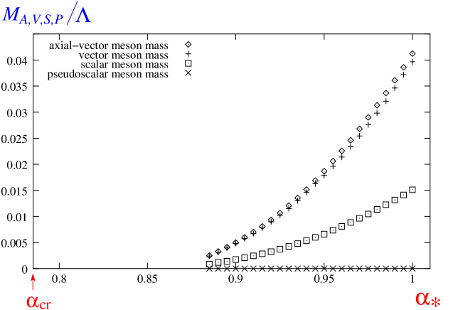
Figure 10: Values of the scalar, pseudoscalar, vector, and axial-vector meson masses for several values of $\alpha_{\ast}$.

This figure shows that the masses of the vector, axial-vector, and scalar bound states go to zero simultaneously as the coupling approaches its critical value (or, equivalently, $N_{f}\rightarrow N_{f}^{\rm crit}$) :

$$M_{S},M_{V},M_{A}\ \rightarrow\ 0\ \quad\mbox{for}\ \ \alpha_{\ast}\ \rightarrow\ \alpha_{\rm cr}\ .$$ (5.75)

Next, to study the critical behavior of $M_{S}$, $M_{V}$, and $M_{A}$ we use the function of the form in Eq. (2.19) and fit the value of $d$ by minimizing

$$\sum_{\alpha_{\ast}}\left|M_{S,V,A}(\alpha_{\ast})-h(\alpha_{\ast})\right|^{2}\ .$$ (5.76)

The resultant best fitted values of $d$ for the scalar, vector, and axial-vector bound states are

$$d_{M_{S}}\simeq 6.2\ ,\ \ d_{M_{V}}\simeq 16.5\ ,\ \ d_{M_{A}}\simeq 17.2\ ,$$ (5.77)

respectively. We also plot (the square of) the ratio of the bound state masses to $F_{P}$ for several values of $\alpha_{\ast}$ in Fig. 11.

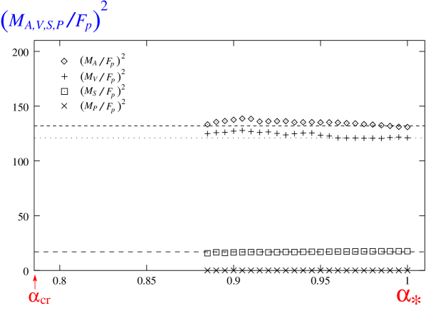
Figure 11: Values of $(M_{A}/F_{P})^{2}$, $(M_{V}/F_{P})^{2}$, $(M_{S}/F_{P})^{2}$ and $(M_{P}/F_{P})^{2}$ for several values of $\alpha_{\ast}$ (indicated by $\Diamond$, $+$, $\Box$, and $\times$, respectively). Dotted lines represent the values of $(M_{A}/F_{P})^{2}=17$, $(M_{V}/F_{P})^{2}=121$, and $(M_{S}/F_{P})^{2}=132$ obtained from Eqs. (5.77) and (2.24).

The dotted lines plotted together with the data in this figure represent the values of the following ratios obtained from Eqs. (5.77) and (2.24) :

$$\left(M_{S}/F_{P}\right)^{2}=17\ ,\ \ \left(M_{V}/F_{P}\right)^{2}=121\ ,\ \ \left(M_{A}/F_{P}\right)^{2}=132\ .$$ (5.78)

This figure clearly shows that all the masses of the scalar, vector, and axial-vector bound states have the same scaling property as that of $F_{P}$ :

$$\frac{M_{S,V,A}}{F_{P}}\ \sim\ {\rm constant}.$$ (5.79)

We can also say that these masses have the same scaling property as that of $\Sigma(m^{2})$ since $F_{P}$ and $\Sigma(m^{2})$ have the same scaling property. Their ratios are summarized as follows:

$$\Sigma^{2}(m^{2}):M_{S}^{2}:M_{V}^{2}:M_{A}^{2}\ \ =\ \ 1\ :\ 2.4\ :\ 17.0\ :\ 18.5\ .$$ (5.80)

One might think that the vector and axial-vector boundstates decay into a fermion and an antifermion since $\ M_{V}^{2}>4\Sigma^{2}(m^{2})\$ and $\ M_{A}^{2}>4\Sigma^{2}(m^{2})$. However, this does not happen: As we noticed above Eq. (2.18), $\ \Sigma(m^{2})\$ is not the pole mass but the dynamical mass defined in the space-like region. Furthermore, as we have shown in section 3, the fermion propagators do not have any poles in the entire complex plane including the time-like axis where the pole mass of fermion should be defined. Thus the vector and axial-vector boundstates do not decay into a fermion and an antifermion.

6 Conclusion and Discussion

In this paper we first pointed out that, when we solve the Schwinger-Dyson (SD) equation in large $N_{f}$ QCD, we do not need to introduce any infrared regularizations for the running coupling since it takes a finite value for all the range of the energy region due to the existence of the IR fixed point. In the case of small $N_{f}$, we have to regularize the infrared divergence of the running coupling, and different schemes of regularizations would give different results. Furthermore, it is difficult to find the regularization which makes the analytic structure of the running coupling simple enough. On the contrary, the solution of the two-loop RGE in large $N_{f}$ QCD is explicitly written in terms of the Lambert $W$ function, and the running coupling does not have any singularities on the complex plane except for the time-like axis when $N_{f}$ is close to $N_{f}^{\rm crit}$. This significant feature of the running coupling in large $N_{f}$ QCD enabled us to solve the SD equation on the complex plane.

Then, we solved the homogeneous Bethe-Salpeter (HBS) equations for the scalar, pseudoscalar, vector, and axial-vector bound states of quark and anti-quark in large $N_{f}$ QCD with the improved ladder approximation in the Landau gauge. In the quark propagator included in the HBS equation, we used the quark mass function obtained from the SD equation with the same approximation, which is needed for the consistency with the chiral symmetry.

We first showed that the HBS equation provides the massless pseudoscalar bound state in the broken phase which is identified with the Nambu-Goldstone boson associated with the spontaneous breaking of the chiral symmetry. Next, we showed that there actually exist vector, axial-vector, and scalar bound states even near the phase transition point in the broken phase, and that their masses decreases as the number of massless quarks $N_{f}$ increases. At the critical point all the masses go to zero, showing the same scaling property as that of the pseudoscalar meson decay constant $F_{P}$ consistently with the picture expected from the conformal phase transition [3, 13].

Let us discuss the pattern of the chiral symmetry restoration by considering the representation of chiral $\mbox{SU}(N_{f})_{\rm L}\times\mbox{SU}(N_{f})_{\rm R}$ of the low-lying mesons extending the analyses done in Refs. [39, 40].

For $N_{f}=3$ the pseudoscalar meson denoted by $\pi$ and the longitudinal axial-vector meson denoted by $A_{1}$ are an admixture of $(8\,,\,1)\oplus(1\,,\,8)$ and $(3\,,\,3^{*})\oplus(3^{*}\,,\,3)$, since the chiral symmetry is spontaneously broken [39, 40]

$$|\pi\rangle = |(3\,,\,3^{*})\oplus(3^{*}\,,\,3)\rangle\sin\psi+|(8\,,\,1)\oplus(1\,,\,8)\rangle\cos\psi\ ,$$

$$|A_{1}(\lambda=0)\rangle = |(3\,,\,3^{*})\oplus(3^{*}\,,\,3)\rangle\cos\psi-|(8\,,\,1)\oplus(1\,,\,8)\rangle\sin\psi\ ,$$ (6.81)

where $\lambda$ denotes the helicity in the collinear frame, and the experimental value of the mixing angle $\psi$ is given by approximately $\psi=\pi/4$ [40]. On the other hand, the longitudinal vector meson denoted by $\rho$ belongs to pure $(8\,,\,1)\oplus(1\,,\,8)$ and the scalar meson denoted by $S$ to pure $(3\,,\,3^{*})\oplus(3^{*}\,,\,3)$:

$$|\rho(\lambda=0)\rangle = |(8\,,\,1)\oplus(1\,,\,8)\rangle\ ,$$

$$|S\rangle = |(3\,,\,3^{*})\oplus(3^{*}\,,\,3)\rangle\ .$$ (6.82)

When the chiral symmetry is restored at the phase transition point, it is natural that the chiral representations coincide with the mass eigenstates: The representation mixing is dissolved. From Eq. (6.81) one can easily see that there are two ways to express the representations in the Wigner phase of the chiral symmetry: The conventional manifestation á la the linear sigma model (called the GL manifestation in Ref. [11]) corresponds to the limit $\psi\rightarrow\pi/2$ in which $\pi$ is in the representation of pure $\ (N_{f}\,,\,N_{f}^{\ast})\oplus(N_{f}^{\ast}\,,\,N_{f})\$ of $\ \mbox{SU}(N_{f})_{\rm L}\times\mbox{SU}(N_{f})_{\rm R}\$ together with the scalar meson, both being the chiral partners:

$$\mbox{(GL)}\qquad\left\{\begin{array}[]{rcl}|\pi\rangle\,,|S\rangle&\rightarrow&|(N_{f}\,,\,N_{f}^{\ast})\oplus(N_{f}^{\ast}\,,\,N_{f})\rangle\ ,\\ |A_{1}(\lambda=0)\rangle\,,|\rho(\lambda=0)\rangle&\rightarrow&|(N_{f}^{2}-1\,,\,1)\oplus(1\,,\,N_{f}^{2}-1)\rangle\ .\end{array}\right.$$ (6.85)

On the other hand, the vector manifestation (VM) [10] corresponds to the limit $\psi\rightarrow 0$ in which the $A_{1}$ goes to a pure $(N_{f}\,,\,N_{f}^{\ast})\oplus(N_{f}^{\ast}\,,\,N_{f})$, now degenerate with the scalar meson in the same representation, but not with $\rho$ in $(N_{f}^{2}-1\,,\,1)\oplus(1\,,\,N_{f}^{2}-1)$:

$$\mbox{(VM)}\qquad\left\{\begin{array}[]{rcl}|\pi\rangle\,,|\rho(\lambda=0)\rangle&\rightarrow&|(N_{f}^{2}-1\,,\,1)\oplus(1\,,\,N_{f}^{2}-1)\rangle\ ,\\ |A_{1}(\lambda=0)\rangle\,,|S\rangle&\rightarrow&|(N_{f}\,,\,N_{f}^{\ast})\oplus(N_{f}^{\ast}\,,\,N_{f})\rangle\ .\end{array}\right.$$ (6.88)

Namely, the degenerate massless $\pi$ and (longitudinal) $\rho$ at the phase transition point are the chiral partners in the representation of $(N_{f}^{2}-1\,,\,1)\oplus(1\,,\,N_{f}^{2}-1)$.

Now, what does our result say on the chiral representation of low-lying mesons? As can be seen from Fig. 11, the resultant values of the masses obtained from the HBS equation roughly satisfies the following relation [40]:

$$M_{A}^{2}+M_{P}^{2}=M_{V}^{2}+M_{S}^{2},$$ (6.89)

for all values of $\alpha_{\ast}$. This relation holds independently of the mixing angle $\psi$ given in Eq. (6.81) when the low-lying mesons saturate the chiral algebra shown in Ref. [40]. Then, it is reasonable to discuss the chiral representation without worrying about the influence of the excited states of the bound states. By using the relation $\tan{\psi}=M_{V}/M_{S}$ [40] and the values of $M_{V}$ and $M_{S}$ obtained from the HBS equation in subsection 5.2, the value of the mixing angle $\psi$ is roughly determined as

$$\ \tan{\psi}=M_{V}/M_{S}\sim 3.$$ (6.90)

This implies that $\pi$ and the longitudinal $A_{1}$ are still admixtures of the pure chiral representation even at the chiral restoration point:

$$|\pi\rangle \rightarrow |(N_{f},N_{f}^{\ast})\oplus(N_{f}^{\ast},N_{f})\ \rangle\sin{\psi}\ +\ |(N_{f}^{2}-1,1)\oplus(1,N_{f}^{2}-1)\ \rangle\cos{\psi},$$

$$|A_{1}\rangle \rightarrow |(N_{f},N_{f}^{\ast})\oplus(N_{f}^{\ast},N_{f})\ \rangle\cos{\psi}\ -\ |(N_{f}^{2}-1,1)\oplus(1,N_{f}^{2}-1)\ \rangle\sin{\psi}.$$

This may suggest the existence of a new type of manifestation of chiral symmetry restoration in large $N_{f}$ QCD which is neither of the GL manifestation nor the simple version of the vector manifestation (VM).

Several comments are in order

In Appendix C, we show the calculations of the coupling constants $F_{V}$, $F_{A}$, and $G_{S}$ of the vector, axial-vector, and scalar bound states to the vector current, axial-vector current, and scalar density. The results shows that they also have the same scaling properties as $F_{P}$. These results indicate that all the dimension-full quantities determined by the infrared dynamics have the same scaling properties, as far as the (improved) ladder approximation is concerned.

Although the masses obtained from the HBS equation satisfy the condition (6.89) needed for the saturation of the chiral algebra, the couplings $F_{P}$, $F_{V}$, and $F_{A}$ do not seem to satisfy the first Weinberg’s sum rule [41]: $F_{P}^{2}+F_{A}^{2}=F_{V}^{2}$. We have not fully understood what this means for the pattern of chiral symmetry restoration. Apparently, reducing the numerical uncertainty will help us to reach the final understanding.

In the present analysis we did not include the effect from the four-fermion interaction which is induced in the case of $\gamma_{m}\simeq 1$ as was conjectured in strong coupling QED [32] and was demonstrated in walking gauge theories [42, 43]. It is not clear at this moment whether or not the qualitative results in the present analysis will be changed when we include such an effect.

In the present analysis we stressed that the running coupling in large $N_{f}$ QCD determined from a two-loop $\beta$-function is expressed as the Lambert $W$ function which enables us to solve the HBS and SD equations with mutual consistency near the critical point. Apparently, this Lambert $W$ function can be used as an infrared regularization to solve the HBS and SD equations with mutual consistency in the case of QCD with small $N_{f}$. It will be very interesting to study meson masses near the chiral phase transition in hot and/or dense QCD by using such an infrared regularization.

We think that it is important to clarify which effective field theory (EFT) describes the new pattern of the chiral symmetry restoration expressed in Eq. (LABEL:new_pattern). Especially, it is very interesting to see how the matching between the EFT and the underlying QCD with large $N_{f}$ can be done to determine bare parameters of the Lagrangian of the EFT.

Appendix A Positronium

In this appendix, to show the validity of the fictitious eigenvalue method for solving the HBS equation explained in subsection 4.3, we calculate the mass of the ortho-positronium which is the vector bound state of the electron and the positron. The same analysis was done in Ref. [38], and here we follow the analysis.

In the weak coupling limit the HBS equation for the ortho-positronium can be solved analytically, and the energy spectrum takes the following form [44]:

$$M_{V}^{(n)}\ =\ 2\,m_{e}\ -\ \frac{m_{e}\,\alpha^{2}}{4\,n^{2}},$$ (A.92)

where $m_{e}$ is the mass of the electron and the positron, and $\alpha=1/137$ is the coupling constant of QED.

We use following parameters in our calculation:

$$[\ \lambda_{U},\ \Lambda_{U}\ ]=[\ -18.5,\ -2.9\ ]\ ,\ \ [\ \lambda_{X},\ \Lambda_{X}\ ]=[\ -10.8,\ 2.2\ ]\ ,$$ (A.93)

$$N_{BS,U}\,=\,N_{BS,X}\,=\,28\ ,\ \ m_{e}=137.0\ .$$ (A.94)

(We used the energy scale which satisfies the relation $m_{e}\alpha=1$ following Ref. [38].) In Fig. 12, we show the resultant values of the fictitious eigenvalue $\lambda$ for several values of the input parameter $M_{V}$.

Figure 12: Fictitious eigenvalues for the positronium.

Finding the point where the smallest $\lambda$ becomes unity, we determine the value of the mass of the ground state $M_{V}^{(1)}$ as the solution of the original HBS equation:

$$M_{V}^{(1)}\ =\ 273.99842.$$ (A.95)

From this the binding energy is calculated as

$$E^{(1)}\ =\ 0.00158.$$ (A.96)

These values are in good agreement with the values $\ M_{V}^{(1)}=273.99817\$ and $E^{(1)}=0.00183$ derived from Eq. (A.92). This shows that our numerical method works well to obtain the mass of the ground state.

Appendix B Bispinor bases for scalar, pseudoscalar, vector, and axial-vector bound states

In this appendix we show the explicit forms of the bispinor bases for the scalar, pseudoscalar, vector, and axial-vector bound states. Here, we use the notation $\hat{q}_{\mu}=q_{\mu}/M_{B}$ with $M_{B}$ being the mass of the bound states, and $[a,b,c]\equiv a[b,c]+b[c,a]+c[a,b]$.

Bispinor base for the scalar bound state ($J^{PC}=0^{++}$) is given by

$$\Gamma_{(S)}^{1}={\bf 1},\ \ \Gamma_{(S)}^{2}=\hbox to0.0pt{\hbox to5.03125pt{\hfil/\hfil}\hss}p,\ \ \Gamma_{(S)}^{3}=\hbox to0.0pt{\hbox to5.55557pt{\hfil/\hfil}\hss}\hat{q}(p\cdot\hat{q}),\ \ \Gamma_{(S)}^{4}=\frac{1}{2}\ [\hbox to0.0pt{\hbox to5.03125pt{\hfil/\hfil}\hss}p,\hbox to0.0pt{\hbox to5.55557pt{\hfil/\hfil}\hss}\hat{q}],$$ (B.97)

and that for the pseudoscalar bound state ($J^{PC}=0^{-+}$) is given by

$$\Gamma_{(P)}^{1}=\gamma_{5},\ \ \Gamma_{(P)}^{2}=\hbox to0.0pt{\hbox to5.03125pt{\hfil/\hfil}\hss}p\ (p\cdot\hat{q})\ \gamma_{5},\ \ \Gamma_{(P)}^{3}=\hbox to0.0pt{\hbox to5.55557pt{\hfil/\hfil}\hss}\hat{q}\ \gamma_{5},\ \ \Gamma_{(P)}^{4}=\frac{1}{2}\ [\hbox to0.0pt{\hbox to5.03125pt{\hfil/\hfil}\hss}p,\hbox to0.0pt{\hbox to5.55557pt{\hfil/\hfil}\hss}\hat{q}]\ \gamma_{5}\ .$$ (B.98)

Furthermore, for the vector bound state ($J^{PC}=1^{--}$) we use

$$\Gamma_{(V)}^{1}=\hbox to0.0pt{\hbox to5.00002pt{\hfil$\epsilon$\hfil}\hss}/,\ \ \Gamma_{(V)}^{2}=\frac{1}{2}[\hbox to0.0pt{\hbox to5.00002pt{\hfil$\epsilon$\hfil}\hss}/,\hbox to0.0pt{\hbox to5.03125pt{\hfil/\hfil}\hss}p](p\cdot\hat{q}),\ \ \Gamma_{(V)}^{3}=\frac{1}{2}[\hbox to0.0pt{\hbox to5.00002pt{\hfil$\epsilon$\hfil}\hss}/,\hbox to0.0pt{\hbox to5.55557pt{\hfil/\hfil}\hss}\hat{q}],\ \ \Gamma_{(V)}^{4}=\frac{1}{3!}[\hbox to0.0pt{\hbox to5.00002pt{\hfil$\epsilon$\hfil}\hss}/,\hbox to0.0pt{\hbox to5.03125pt{\hfil/\hfil}\hss}p,\hbox to0.0pt{\hbox to5.55557pt{\hfil/\hfil}\hss}\hat{q}],$$ (B.99)

$$\Gamma_{(V)}^{5}=(\epsilon\cdot p),\ \ \Gamma_{(V)}^{6}=\hbox to0.0pt{\hbox to5.03125pt{\hfil/\hfil}\hss}p(\epsilon\cdot p),\ \ \Gamma_{(V)}^{7}=\hbox to0.0pt{\hbox to5.55557pt{\hfil/\hfil}\hss}\hat{q}(p\cdot\hat{q})(\epsilon\cdot p),\ \ \Gamma_{(V)}^{8}=\frac{1}{2}[\hbox to0.0pt{\hbox to5.03125pt{\hfil/\hfil}\hss}p,\hbox to0.0pt{\hbox to5.55557pt{\hfil/\hfil}\hss}\hat{q}](\epsilon\cdot p),$$

and for the axial-vector bound state ($J^{PC}=1^{++}$)

$$\Gamma_{(A)}^{1} = \hbox to0.0pt{\hbox to5.00002pt{\hfil$\epsilon$\hfil}\hss}/\ \gamma_{5},\ \ \ \Gamma_{(A)}^{2}=\frac{1}{2}[\hbox to0.0pt{\hbox to5.00002pt{\hfil$\epsilon$\hfil}\hss}/,\hbox to0.0pt{\hbox to5.03125pt{\hfil/\hfil}\hss}p]\gamma_{5},\ \ \ \Gamma_{(A)}^{3}=\frac{1}{2}[\hbox to0.0pt{\hbox to5.00002pt{\hfil$\epsilon$\hfil}\hss}/,\hbox to0.0pt{\hbox to5.55557pt{\hfil/\hfil}\hss}\hat{q}]\ (p\cdot\hat{q})\ \gamma_{5},$$

$$\Gamma_{(A)}^{4} = \frac{1}{3!}[\hbox to0.0pt{\hbox to5.00002pt{\hfil$\epsilon$\hfil}\hss}/,\hbox to0.0pt{\hbox to5.03125pt{\hfil/\hfil}\hss}p,\hbox to0.0pt{\hbox to5.55557pt{\hfil/\hfil}\hss}\hat{q}]\ \gamma_{5},\ \ \ \Gamma_{(A)}^{5}=(\epsilon\cdot p)\ (p\cdot\hat{q})\ \gamma_{5},\ \ \ \Gamma_{(A)}^{6}=\hbox to0.0pt{\hbox to5.03125pt{\hfil/\hfil}\hss}p(\epsilon\cdot p)\ \gamma_{5},$$

$$\Gamma_{(A)}^{7} = \hbox to0.0pt{\hbox to5.55557pt{\hfil/\hfil}\hss}\hat{q}\ (\epsilon\cdot p)\ (p\cdot\hat{q})\ \gamma_{5},\ \ \ \Gamma_{(A)}^{8}=\frac{1}{2}[\hbox to0.0pt{\hbox to5.03125pt{\hfil/\hfil}\hss}p,\hbox to0.0pt{\hbox to5.55557pt{\hfil/\hfil}\hss}\hat{q}](\epsilon\cdot p)\ (p\cdot\hat{q})\ \gamma_{5}.$$ (B.100)

Appendix C Coupling constants to currents and scalar density

In this subsection we calculate coupling constants $F_{V}$, $F_{A}$, and $G_{S}$ of the vector, axial-vector, and scalar bound states to the vector current, axial-vector current, and scalar density. They are defined by

$$\langle\ 0\ |\ \bar{\psi}(0)\ \gamma^{\mu}\ \frac{\lambda_{a}}{2}\ \psi(0)\ |\ V_{b}(q,\epsilon)\ \rangle\ = \ \delta_{ab}\ F_{V}\ M_{V}\ \epsilon^{\mu},$$ (C.101)

$$\langle\ 0\ |\ \bar{\psi}(0)\ \gamma^{\mu}\ \gamma_{5}\ \frac{\lambda_{a}}{2}\ \psi(0)\ |\ A_{b}(q,\epsilon)\ \rangle\ = \ \delta_{ab}\ F_{A}\ M_{A}\ \epsilon^{\mu},$$ (C.102)

$$\langle\ 0\ |\ \bar{\psi}(0)\ \frac{\lambda_{a}}{2}\ \psi(0)\ |\ S_{b}(q,\epsilon)\ \rangle\ = \ \delta_{ab}\ G_{S},$$ (C.103)

where $\lambda_{a}$ is the flavor matrix normalized as $\mbox{tr}[\lambda_{a}\lambda_{b}]=2\delta_{ab}$.

By using the BS amplitudes for the vector bound state, $F_{V}$ is expressed as

$$F_{V}M_{V}\ =\ -\ \frac{\sqrt{2}\,i\,N_{c}}{\pi^{3}}\ \int_{0}^{\infty}du\int_{0}^{\infty}dx\Bigg{[}\ x^{2}\,\chi^{1}(u,x)\ -\ \frac{x^{4}}{3}\,\chi^{6}(u,x)\ \Bigg{]}\ .$$ (C.104)

In the above expression, the normalization of the BS amplitudes $\chi^{i}$ are determined by the following normalization condition [14]:

$$2M_{V}\,\delta_{\epsilon\epsilon^{\prime}}=iN_{c}\int\frac{d^{4}p}{(2\pi)^{4}}\Bigg{[}\,\bar{\chi}(p;q,\epsilon)\,\frac{\partial T(p;q)}{\partial M_{V}}\,\chi(p;q,\epsilon^{\prime})\,\Bigg{]}\ .$$ (C.105)

Here, we notice again that $T(p;q)$ has no singularity although the fermion propagator $S_{F}$ has a branch cut in the time-like region. So the integral in Eq. (C.105) is well-defined. Once we have obtained $M_{V}$ and the corresponding BS amplitudes by solving the HBS equation, we can calculate $F_{V}$ from Eq. (C.104). We can also calculate $F_{A}$ and $G_{S}$ in a similar way. In Fig. 13 (a) we show the values of $F_{V}$, $F_{A}$, and $G_{S}$ together with $F_{P}$ for several values of $\alpha_{\ast}$.

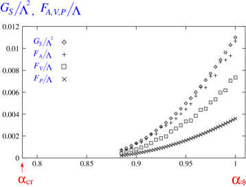
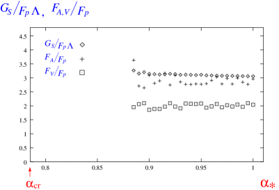
(a)                                                               (b)

Figure 13: Values of  (a) $F_{V}$, $F_{A}$, $G_{S}$, and $F_{P}$ and  (b) $G_{S}/F_{P}$, $F_{V}/F_{P}$, and $F_{A}/F_{P}$ for several values of $\alpha_{\ast}$.

To see the scaling properties, we plot the ratio of $F_{V}$, $F_{A}$, and $G_{S}$ to $F_{P}$ in Fig. 13 (b). This figure shows that $F_{V}$, $F_{A}$, and $G_{S}$ have the same scaling properties as that of $F_{P}$.

Appendix D Uncertainties for numerical calculations

To solve the HBS equation for the bound states numerically, we introduced the UV and IR cutoffs and converted the HBS equation into a linear eigenvalue equation by discretizing the integral. As we have discussed in subsection 5.2, we adjust the values of the UV and IR cutoffs in such a way that the dominant supports of the integrands of the decay constant in Eq. (C.104) and the normalization condition in Eq. (C.105) lie in the energy region between the UV and IR cutoffs. In Figs. 14 and 15 we show those integrands for $\alpha_{\ast}=0.885$ and $1.0$ in the case of the vector bound state.

(a)                                                        (b)

Figure 14: Integrands of (a) the decay constant in Eq. (C.104) and (b) the normalization condition in Eq. (C.105) for $\alpha_{\ast}=0.885$.

(a)                                                        (b)

Figure 15: Integrands of  (a)  the decay constant in Eq. (C.104) and  (b)  the normalization condition in Eq. (C.105) for $\alpha_{\ast}=1.0$.

These figures show that the dominant supports lie in the lower energy region for smaller value of $\alpha_{\ast}$, and that the present choices in Eqs. (5.70) and (5.71) covers the supports. For other values of $\alpha_{\ast}$ used in the present analysis we have checked that the dominant supports always lie within the energy region between the UV and IR cutoffs chosen as in Eqs. (5.70) and (5.71).

As for the numbers of the discretization, due to the limitation of the computer resources we used $N_{BS,U}=20$ and $N_{BS,X}=55$ as shown in Eq. (5.73). Here we study the dependences of the mass and the decay constant of the vector bound state on the size of discretization. We show the typical values of the mass in Fig. 16 (a) and those of the decay constant in Fig. 16 (b) for five choices of the size of the discretization, $(N_{BS,U},N_{BS,X})=(14,28)$, $(16,32)$, $(18,36)$, $(20,40)$, and $(20,55)$.

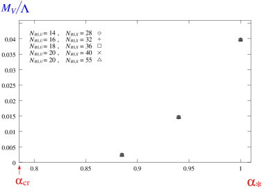
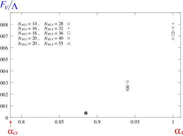
(a)                                                                  (b)

Figure 16: Typical values of  (a)  $M_{V}/\Lambda$ and  (b) $F_{V}/\Lambda$ for five choices of the size of discretization, $(N_{BS,U},N_{BS,X})=(14,28)$, $(16,32)$, $(18,36)$, $(20,40)$, and $(20,55)$.

Figure 16 (a) clearly shows that the choice $(N_{BS,U},N_{BS,X})=(20,55)$ is large enough to obtain the mass of the vector bound state. On the other hand, Fig. 16 (b) shows that there are still uncertainties in the value of the decay constant which come from the size of the discretization. Apparently, this uncertainty from the size of discretization is the dominant part of the numerical uncertainties in the present analysis.

References

- [1] T. Banks and A. Zaks, Nucl. Phys. B 196, 189 (1982).
- [2] T. Appelquist, J. Terning and L. C. Wijewardhana, Phys. Rev. Lett. 77, 1214 (1996) [arXiv:hep-ph/9602385].
- [3] V. A. Miransky and K. Yamawaki, Phys. Rev. D 55, 5051 (1997) [Erratum-ibid. D 56, 3768 (1997)] [arXiv:hep-th/9611142].
- [4] T. Appelquist, A. Ratnaweera, J. Terning and L. C. Wijewardhana, Phys. Rev. D 58, 105017 (1998) [arXiv:hep-ph/9806472].
- [5] J. B. Kogut and D. K. Sinclair, Nucl. Phys. B 295, 465 (1988); F. R. Brown, H. Chen, N. H. Christ, Z. Dong, R. D. Mawhinney, W. Schaffer and A. Vaccarino, Phys. Rev. D 46, 5655 (1992); Y. Iwasaki, K. Kanaya, S. Sakai and T. Yoshie, Phys. Rev. Lett. 69, 21 (1992); Y. Iwasaki, K. Kanaya, S. Kaya, S. Sakai and T. Yoshie, Nucl. Phys. Proc. Suppl. 53, 449 (1997); Prog. Theor. Phys. Suppl. 131, 415 (1998).
- [6] R. Oehme and W. Zimmermann, Phys. Rev. D 21, 471 (1980).
- [7] M. Velkovsky and E. Shuryak, Phys. Lett. B 437, 398 (1998).
- [8] T. Hatsuda and T. Kunihiro, Phys. Rept. 247, 221 (1994); R. D. Pisarski, hep-ph/9503330; G.E. Brown and M. Rho, Phys. Rept. 269, 333 (1996); F. Wilczek, hep-ph/0003183; G. E. Brown and M. Rho, Phys. Rept. 363, 85 (2002) [arXiv:hep-ph/0103102].
- [9] M. Harada and K. Yamawaki, Phys. Rev. Lett. 83, 3374 (1999) [arXiv:hep-ph/9906445].
- [10] M. Harada and K. Yamawaki, Phys. Rev. Lett. 86, 757 (2001) [arXiv:hep-ph/0010207].
- [11] M. Harada and K. Yamawaki, to appear in Phys. Rept. [arXiv:hep-ph/0302103].
- [12] M. Bando, T. Kugo, S. Uehara, K. Yamawaki and T. Yanagida, Phys. Rev. Lett. 54, 1215 (1985); M. Bando, T. Kugo and K. Yamawaki, Phys. Rept. 164, 217 (1988).
- [13] R. S. Chivukula, Phys. Rev. D 55, 5238 (1997) [arXiv:hep-ph/9612267].
- [14] N. Nakanishi, Prog. Theor. Phys. Suppl. 43, 1 (1969).
- [15] T. Kugo, in Proc. of 1991 Nagoya Spring School on Dynamical Symmetry Breaking, Nakatsugawa, Japan, 1991, ed. K. Yamawaki (World Scientific, Singapore, 1992).
- [16] V. A. Miransky, “Dynamical symmetry breaking in quantum field theories,” Singapore, Singapore: World Scientific (1993) 533 p.
- [17] T. Maskawa and H. Nakajima, Prog. Theor. Phys. 52, 1326 (1974); T. Maskawa and H. Nakajima, Prog. Theor. Phys. 54, 860 (1975); M. Bando, M. Harada and T. Kugo, Prog. Theor. Phys. 91, 927 (1994) [arXiv:hep-ph/9312343].
- [18] T. Kugo and M. G. Mitchard, Phys. Lett. B 282, 162 (1992).
- [19] T. Kugo and M. G. Mitchard, Phys. Lett. B 286, 355 (1992).
- [20] M. Bando, M. Harada and T. Kugo, Prog. Theor. Phys. 91, 927 (1994) [arXiv:hep-ph/9312343].
- [21] K. Higashijima, Phys. Rev. D 29, 1228 (1984).
- [22] V. A. Miransky, Sov. J. Nucl. Phys. 38, 280 (1983) [Yad. Fiz. 38, 468 (1983)].
- [23] K. I. Aoki, M. Bando, T. Kugo, M. G. Mitchard and H. Nakatani, Prog. Theor. Phys. 84, 683 (1990).
- [24] K. I. Aoki, M. Bando, T. Kugo and M. G. Mitchard, Prog. Theor. Phys. 85, 355 (1991).
- [25] C. D. Roberts and S. M. Schmidt, Prog. Part. Nucl. Phys. 45, S1 (2000) [arXiv:nucl-th/0005064].
- [26] T. Kugo, M. G. Mitchard and Y. Yoshida, Prog. Theor. Phys. 91, 521 (1994) [arXiv:hep-ph/9312267].
- [27] P. Maris, C. D. Roberts and P. C. Tandy, Phys. Lett. B 420, 267 (1998) [arXiv:nucl-th/9707003].
- [28] K. I. Aoki, T. Kugo and M. G. Mitchard, Phys. Lett. B 266, 467 (1991).
- [29] K. Naito, K. Yoshida, Y. Nemoto, M. Oka and M. Takizawa, Phys. Rev. C 59, 1095 (1999) [arXiv:hep-ph/9805243]; K. Naito and M. Oka, Phys. Rev. C 59, 542 (1999) [arXiv:hep-ph/9805258].
- [30] R. Alkofer, P. Watson and H. Weigel, Phys. Rev. D 65, 094026 (2002) [arXiv:hep-ph/0202053].
- [31] E. Gardi and M. Karliner, Nucl. Phys. B 529, 383 (1998) [arXiv:hep-ph/9802218]; E. Gardi, G. Grunberg and M. Karliner, JHEP 9807, 007 (1998) [arXiv:hep-ph/9806462].
- [32] C. N. Leung, S. T. Love and W. A. Bardeen, Nucl. Phys. B 273, 649 (1986); Nucl. Phys. B 323, 493 (1989).
- [33] T. Appelquist, K. D. Lane and U. Mahanta, Phys. Rev. Lett. 61, 1553 (1988); H. Georgi, E. H. Simmons and A. G. Cohen, Phys. Lett. B 236, 183 (1990).
- [34] R. M. Corless, G. H. Gonnet, D. G. E. Hare, D. J. Jeffrey and D. E. Knuth, Adv. Comput. Math. 5, 329 (1996).
- [35] H. Pagels and S. Stokar, Phys. Rev. D 20, 2947 (1979).
- [36] B. Holdom, Phys. Lett. B 150, 301 (1985); K. Yamawaki, M. Bando and K. Matumoto, Phys. Rev. Lett. 56, 1335 (1986); T. Akiba and T. Yanagida, Phys. Lett. B 169, 432 (1986); T.W. Appelquist, D. Karabali and L.C.R. Wijewardhana, Phys. Rev. Lett. 57, 957 (1986).
- [37] T. Kugo and Y. Yoshida, Soryushiron Kenkyu 91, B26 (1995); Y. Yoshida, Ph.D thesis, Kyoto University (1995)
- [38] M. Harada and Y. Yoshida, Phys. Rev. D 53, 1482 (1996) [arXiv:hep-ph/9505206].
- [39] F. J. Gilman and H. Harari, Phys. Rev. 165, 1803 (1968).
- [40] S. Weinberg, Phys. Rev. 177, 2604 (1969).
- [41] S. Weinberg, Phys. Rev. Lett. 18, 507 (1967).
- [42] K.-I. Kondo, S. Shuto and K. Yamawaki, Mod. Phys. Lett. A 6, 3385 (1991).
- [43] K. I. Aoki, K. Morikawa, J. I. Sumi, H. Terao and M. Tomoyose, Prog. Theor. Phys. 102, 1151 (1999) [arXiv:hep-th/9908042].
- [44] See, for example, C. Itzykson and J. B. Zuber, Quantum Field Theory (McGraw-Hill, New York, 1980).