Spin-Orbit and Tensor Forces in Heavy-quark Light-quark Mesons: Implications of the New $D_{s}$ State at 2.32 GeV

Abstract

We consider the spectroscopy of heavy-quark light-quark mesons with a simple model based on the non-relativistic reduction of vector and scalar exchange between fermions. Four forces are induced: the spin-orbit forces on the light and heavy quark spins, the tensor force, and a spin-spin force. If the vector force is Coulombic, the spin-spin force is a contact interaction, and the tensor force and spin-orbit force on the heavy quark to order $1/m_{1}m_{2}$ are directly proportional. As a result, just two independent parameters characterize these perturbations. The measurement of the masses of three p-wave states suffices to predict the mass of the fourth. This technique is applied to the $D_{s}$ system, where the newly discovered state at 2.32 GeV provides the third measured level, and to the $D$ system. The mixing of the two $J^{P}=1^{+}$ p-wave states is reflected in their widths and provides additional constraints. The resulting picture is at odds with previous expectations and raises new puzzles.

I Introduction

Mesons composed of one light quark and one heavy quark are quite analogous to the hydrogen atom dgg and can be analyzed using the traditional methods bethe-salpeter . The fine and hyperfine structures have direct analogues in meson spectroscopy, but the confinement of quarks requires that potential cannot be purely Coulombic. A convenient phenomenological approach is to postulate that there are two separate static potentials, one arising as the zeroth component of a vector potential and the other as a Lorentz scalar. Asymptotic freedom suggests that the vector potential be Coulombic, while confinement suggests that the scalar be a linear potential. Such models have had reasonable success in describing the spectroscopy of the $D$, $D_{s}$, $B$, and $B_{s}$ systems godfrey-isgur ; godfrey-kokoski ; isgur-wise ; eichten-hill-quigg ; dipierro-eichten .

The recently discovered state with a mass of 2.32 GeV decaying to $D_{s}\pi^{0}$ babar appears to be a $c{\overline{s}}$ p-wave meson with $J^{P}=0^{+}$. Typical predictions for its mass were near 2.5 GeV, above the threshold for the strong decay to $DK$. Here we analyze the p-wave $c{\overline{s}}$ and $c{\overline{u}}/{\overline{d}}$ mesons in a simple model that is more general, though less predictive, than the models described above. It is more general in that we do not specialize to a scalar potential that is linear.

Our concern here is restricted to the p-wave states. While our primary interest is in the $D_{s}$ system, we consider as well the analogous non-strange $D$ mesons. It is not only the mass spectrum that needs to be addressed, but also the pattern of decay widths. The early studies, which predicted a much higher mass for the $J^{P}=0^{+}$ $c{\overline{s}}$, were successful in explaining the narrow width of the observed $J^{P}=1^{+}$ states in both the $D$ and $D_{s}$ systems. We find that the combined constraints of the mass spectrum as now known (though lacunae remain) and the decay patterns make it difficult to find a consistent picture of the p-wave charmed strange and non-strange mesons.

By analogy with the hydrogen atom, a convenient classification of states is given in terms of ${\bm{j}}={\bm{\ell}}+{\bm{s}}_{1}$, where ${\bm{\ell}}$ is the orbital angular momentum and ${\bm{s}}_{1}$ is the spin of the light quark. The light-quark angular momentum ${\bm{j}}$ is conserved in the limit in which the heavy-quark mass, $m_{2}$, goes to infinity. For p-wave states, the values of $j$ are $3/2$ and $1/2$. These levels are split by the ordinary spin-orbit force. The hyperfine structure is proportional to $1/m_{1}m_{2}$ and includes the spin-orbit coupling of the heavy quark, a spin-spin interaction, and the tensor force. All these contribute to further reducing the degeneracy so that ${\bm{J}}={\bm{j}}+{\bm{s}}_{2}$ is conserved, but not ${\bm{j}}$ alone. The result is four distinct states with $J^{P}=0^{+},1^{+},1^{+},$ and $2^{+}$. The two $J^{P}=1^{+}$ states are mixtures of $j=3/2$ and $j=1/2$. The $J=2$ and $J=0$ states are pure $S=1$ states, where ${\bm{S}}={\bm{s}}_{1}+{\bm{s}}_{2}$ is the total spin. The $J=1$ eigenstates are mixtures of spin-triplet and spin-singlet.

The p-wave $D$ mesons decay by pion emission. The $2^{+}$ state decays through d-wave emission to the ground state $0^{-}$, $D$ or to the $1^{-}$, $D^{*}$. The $1^{+}$ states can decay, in principle, either by d-wave or s-wave pion emission. The limited phases space favors the s-wave decay. However, the decay of $j=3/2$ state to the $D^{*}$, which has $j=1/2$, is forbidden to the extent that ${\bm{j}}$ is conserved. Indeed, the $J^{P}=1^{+}$ state at 2.422 GeV is narrow.

For p-wave $D_{s}$ mesons, decay by pion emission is forbidden by isospin invariance. The $D_{s}$ states at 2.572 GeV and 2.536 GeV decay to $DK$ and $D^{*}K$. In a fashion analogous to the pattern in the $D$ system, the $J^{P}=1^{+}$ state at 2.536 GeV is also narrow.

II Spectrum for P States

We base our analysis on the quasi-static potential, including the spin-dependent forces, which computed from the Lorentz-invariant fermion-antifermion scattering amplitude using Feynman diagrams, replacing the vector or scalar propagators by the Fourier transforms of the postulated potentials, $S(r)$ and $V(r)$. In this way, neglecting velocity-dependent, but spin-independent terms, we find

$${\cal V}_{quasi-static} = V+S+\left({V^{\prime}-S^{\prime}\over r}\right){\bm{\ell}}\!\cdot\!\left({\bm{\sigma}_{1}\over 4m_{1}^{2}}+{\bm{\sigma}_{2}\over 4m_{2}^{2}}\right)+\left({V^{\prime}\over r}\right){\bm{\ell}}\!\cdot\!\left({\bm{\sigma}_{1}+\bm{\sigma}_{2}\over 2m_{1}m_{2}}\right)$$ (1)

$$\qquad\qquad\qquad\qquad+{1\over 12m_{1}m_{2}}\left({V^{\prime}\over r}-V^{\prime\prime}\right)S_{12}+{1\over 6m_{1}m_{2}}\nabla^{2}V\,\bm{\sigma}_{1}\!\cdot\!\bm{\sigma}_{2}$$

where the tensor force operator is

$$S_{12}=3\,\bm{\sigma}_{1}\!\cdot\!\hat{\bm{r}}\,\bm{\sigma}_{2}\!\cdot\!\hat{\bm{r}}-\bm{\sigma}_{1}\!\cdot\!\bm{\sigma}_{2}.$$ (2)

We imagine solving the corresponding differential equation with the potential $V+S$, then computing the fine structure and hyperfine structure perturbatively. We work consistently only to order $1/m_{2}$. In general, there are four independent matrix elements to consider, $\langle(V^{\prime}-S^{\prime})/r\rangle$, $\langle V^{\prime}/r\rangle$, $\langle-V^{\prime\prime}+V^{\prime}/r\rangle$, and $\langle\nabla^{2}V\rangle$. However, if $V$ is Coulombic, $-V^{\prime\prime}+V^{\prime}/r=3V^{\prime}/r$ and $\langle\nabla^{2}V\rangle$ vanishes except for s waves, where it gives a contact interaction. It follows that for Coulombic $V$ and for $\ell>0$, there are only two independent matrix elements. Three measured p-wave masses will give two splittings, which will determine the matrix elements and allow us to predict the mass of the fourth p-wave state.

The mass operator for the splittings of the four states of any multiplet of orbital angular momentum different from zero can be written (to order $1/m_{2}$)rosner

$$M=\lambda{\bm{\ell}}\cdot{\bm{s}}_{1}+4\tau{\bm{\ell}}\cdot{\bm{s}}_{2}+\tau S_{12}$$ (3)

with the notation

$$\lambda = {1\over 2m_{1}^{2}}\left[{V^{\prime}\over r}\left(1+{2m_{1}\over m_{2}}\right)-{S^{\prime}\over r}\right]$$

$$\tau = {1\over 4m_{1}m_{2}}{V^{\prime}\over r}.$$ (4)

In practice, we shall apply this operator to p-wave states for the $D$ or $D_{s}$ system. Henceforth, we will use $\lambda$ and $\tau$ to indicate the expectation values of the quantities in Eq. (4). The values of $\lambda$ and $\tau$ will be different for the $D$ and $D_{s}$ systems. For the assumed attractive, Coulombic $V$, the tensor-force energy $\tau$ is manifestly positive. However, the spin-orbit energy $\lambda$ can be either positive or negative, depending on the relation between the potentials $V$ and $S$.

Because there is no single basis that diagonalizes all the interactions, we need to fix one basis, then calculate the mixing between the two $J=1$ states. We choose the basis in which $j^{2}$ is diagonal. The eigenstates $|J,\,j,\,m\rangle$ of $J^{2}$, $j^{2}$ and $J_{z}$ can be written in terms of eigenstates of $J^{2}$, $S^{2}$, and $J_{z}$, or in terms of eigenstates of $J^{2}$, $(\bm{j}^{\prime})^{2}=(\bm{\ell}+\bm{s}_{2})^{2}$ and $J_{z}$. The details are given in the Appendix.

Up to an additive constant common to the four p-wave states, the masses of the $J=2$ and $J=0$ states are

$$M_{2}={\lambda\over 2}+{8\over 5}\tau;\qquad M_{0}=-\lambda-8\tau$$ (5)

while the masses of the two $J=1$ state are obtained by diagonalizing the matrix in the $|J,\,j,\,m\rangle$ basis

$$\left(\begin{array}[]{cc}{\lambda\over 2}-\frac{8}{3}\tau&-\frac{2\sqrt{2}}{3}\tau\\[14.45377pt] -\frac{2\sqrt{2}}{3}\tau&-\lambda+\frac{8}{3}\tau\end{array}\right)$$ (6)

The two eigenmasses for $J=1$ are then

$$M_{1\pm} = -\frac{\lambda}{4}\pm\sqrt{\frac{\lambda^{2}}{16}+\frac{1}{2}(\lambda-4\tau)^{2}}$$ (7)

The eigenmasses are shown as functions of $\lambda/\tau$ in Fig. 1. Also shown is the $j=1/2$ fraction of the higher mass $J^{P}=1^{+}$ state. The vertical bands correspond to theoretical models and to data, as explained in the next section.

If we define the mass splittings among three of the four states,

$$D_{2} = M_{2}-M_{0}$$

$$D_{1} = M_{1}-M_{0}$$ (8)

we find

$$\tau = \frac{10}{87}D_{2}-\frac{2}{29}D_{1}$$

$$\qquad\pm\sqrt{\left(\frac{10}{87}D_{2}-\frac{2}{29}D_{1}\right)^{2}+\frac{5}{232}(D_{1}^{2}-D_{1}D_{2})}$$

$$\lambda = \frac{2}{3}D_{2}-\frac{32}{5}\tau$$ (9)

A very strong scalar potential $S$ leads to “inversion,” namely the $j=1/2$ states lying above the $j=3/2$ states.

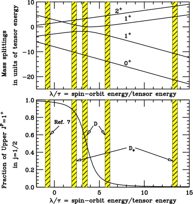
Figure 1: Upper: the energy-levels for the four p-wave states as a function of the ratio of the spin-orbit to tensor energies, in units of the tensor energy. Lower: the percentage of the more massive $J^{P}=1^{+}$ state that comes from the $j=1/2$ state. The $D$ masses are from rpp ; belle and the $D_{s}$ masses from rpp ; babar .

III Application to the $D$ and $D_{s}$ Systems

Using the formulae of the preceding Section, we can use the measured masses of three p-wave states to predict the fourth. Alternatively, we can take three masses that are predicted theoretically and confirm that we find the fourth predicted mass. Applying this to the $D$ and $D_{s}$ systems as given in Ref. dipierro-eichten we indeed find congruence and determine the values of $\lambda$ and $\tau$ shown in Table 1. The leftmost vertical bar in Fig. 1 indicates the range found in Ref. dipierro-eichten . The negative value of $\lambda$ is indicative of inversion.

The result of inversion is that the higher-mass $J^{P}=1^{+}$ state actually lies above the $2^{+}$ state. This prediction is contradicted by the reports from Belle belle of $J^{P}=1^{+}$ state at 2.400 GeV. Using the well established $D$ states at 2.459 GeV and 2.422 GeV, and the reported $J^{P}=0^{+}$ at 2.290 GeV in our Eq. (3) leads to two solutions, labeled A and B in Table 1. Both give masses near the observed state at 2.400 GeV. From the lower graph in Fig. 1 we see that the solution with the higher value of $\lambda/\tau$ results in the higher-mass $J^{P}=1^{+}$ state (2.422 GeV) being nearly entirely $j=3/2$, while the lower value (Solution A), would give it nearly equal contributions from $j=1/2$ and $j=3/2$.

Table 1: Masses of the various p-wave states in the $D$ and $D_{s}$ systems and the spin-orbit and tensor energies. The experimental masses for the $D$ states at 2.400 GeV and 2.290 GeV are from Ref. belle . The mass of the $D_{s}$ state at 2.317 GeV is from Ref. babar . The values of $\lambda$ and $\tau$ for Ref. dipierro-eichten were obtained by fitting their mass spectrum with the ansatz of Eq. 3. The square brackets indicate values that were used as inputs to the fits that determined the remaining mass and the values of $\lambda$ and $\tau$. At the time of Ref. dipierro-eichten only the masses of the $2^{+}$ states and the $D_{1}(2420)$ and $D_{s1}(2535)$ were known.

	Exp.	Theory
	Ref. rpp ; belle ; babar	Sol. A	Sol. B	Ref. dipierro-eichten
$D$ mesons
$M(2^{+})$(GeV)	2.459	[2.459]	[2.459]	2.460
$M(1^{+})$(GeV)	2.400	2.400	2.385	2.490
$M(1^{+})$(GeV)	2.422	[2.422]	[2.422]	2.417
$M(0^{+})$(GeV)	2.290	[2.290]	[2.290]	2.377
$\lambda$ (MeV)		39	54	$-11$
$\tau$ (MeV)		11	9	11
$D_{s}$ mesons
$M(2^{+})$(GeV)	2.572	[2.572]	[2.572]	2.581
$M(1^{+})$(GeV)		2.480	2.408	2.605
$M(1^{+})$(GeV)	2.536	[2.536]	[2.536]	2.535
$M(0^{+})$(GeV)	2.317	[2.317]	[2.317]	2.487
$\lambda$ (MeV)		43	115	$-7$
$\tau$ (MeV)		20	9	11

We can differentiate between the two solutions, both for $D$ and $D_{s}$ by considering the widths. The experimental widths and theoretical estimates are shown in Table 2. The theoretical estimates are obtained from dipierro-eichten after making phase-space corrections. The widths for s-wave and d-wave decay are shown separately for the $J^{P}=1^{+}$ states. The proper combination depends on the mixing of the $j=3/2$ and $j=1/2$ states.

Table 2: Decay widths of p-wave $D$ and $D_{s}$ states in MeV. The theoretical values are derived from dipierro-eichten using phase-space corrections to adjust for the masses known now. The widths shown for the $D_{2}^{*}(2460)$ states are obtained from the total width of $23\pm 5$ $0^{-}$ and the measured rpp ratio $\Gamma(D^{+}\pi^{-})/\Gamma(D^{*+}\pi^{-})=2.3\pm 0.6$. For the $D_{sJ}(2573)$ we have assigned the entire width to the decay to $D(1865)K$ since the decay to $D^{*}(2007)K$ has not been seen.

	Exp.	Theory:
	rpp ; belle	s-wave	d-wave
$D$ mesons
$D_{2}^{*}(2460)\to D(1865)\pi$	$16\pm 4$		16
$D_{2}^{*}(2460)\to D^{*}(2007)\pi$	$7\pm 3$		9
$D_{1}(2422)\to D^{*}(2007)\pi$	$18.9{+4.6\atop-3.5}$	90	10
$D_{1}(2400)\to D^{*}(2007)\pi$	$380\pm 100\pm 100$	100
$D_{0}^{*}(2290)$	$305\pm 30\pm 25$	100
$D_{s}$ mesons
$D_{2}^{*}(2573)\to D(1865)K$	$15{+5\atop-4}$		9
$D_{2}^{*}(2573)\to D^{*}(2007)K$	$-$		1.4
$D_{1}(2535)\to D^{*}(2007)K$	$<2.3$	100	0.3

Referring to Fig. 1 and Table 1, we see that the model of dipierro-eichten , which has $\lambda<0$, has the $J=1$ state that is nearly pure $j=1/2$ above the $J=2$ state. The lower $J=1$ state is identified with the $D_{1}(2420)$. Because it is nearly entirely $j=3/2$ its decay by pion emission must be d-wave. This causes a suppression that conforms to the measured width. However, the mass spectrum predicted by Ref. dipierro-eichten is not in good agreement with the data. Of our two solutions for the $D$ data, only one has a large value of $\lambda/\tau$ as needed to make the lower mass $J=1$ state broad, as required by the data.

Turning to the $D_{s}$ system, we find a similar situation. While Ref. dipierro-eichten would have $\lambda<0$, the known masses, which now include the $0^{+}$ state at 2.32 GeV, require $\lambda>0$. Indeed, to suppress the width of the $D_{s}(2535)$, a large $\lambda$ is needed. This is the case for Solution A, where the mass predicted for the fourth p-wave state is 2408 MeV. One of us (JDJ) notes that in Ref. babar , there is an apparent signal in the invariant mass of $D_{s}\pi^{0}\gamma$ 2.46 GeV. This would be consistent with a $J^{P}=1^{+}$ state decaying through $D_{sJ}^{*}(2317)\gamma$ or through $D^{*}_{s}(2112)\pi^{0}$. The mass fits better with Solution A of Table 1, but the narrow width of the $D_{s1}(2535)$ favors Solution B.

Both the $D$ and $D_{s}$ systems show deviations from the pattern anticipated by potential models. While “inversion”, i.e. $\lambda<0$, has been a favored prediction, it is not in agreement with the data. This suggests that the ansatz taken for the potentials $V$ and $S$ may not be as simple as assumed. We have allowed $S$ to be any potential, while requiring that $V$ be Coulombic; Ref. dipierro-eichten required that $S$ be linear. Relaxing that restriction might lead to improved agreement with the data for this highly predictive approach, which actually uses the solutions to the Dirac equation. On the other hand, even with the flexibility allowed in our approach, the resulting picture is not entirely attractive. We expect the confining potential to be quite important since the p-wave states are not concentrated at the origin. This would lead to a suppression of $\lambda$ through the contribution of the $-S^{\prime}/r$ term. This is not borne out by the values of $\lambda$ we deduce.

The discovery of the $D_{sJ}^{*}(2317)$ has provided an important clue to heavy-quark light-quark spectroscopy by nailing down a p-wave state with $j=1/2$. Puzzles remain. The anticipated discovery of the accompanying $j=1/2$ state with $J=1$ should add important new information, but it is not likely to resolve all the questions we have described.

IV Appendix

The relations betweeen the three bases that diagonalize $j^{2}$, $j^{\prime 2}$, and $S^{2}$ are

$$\begin{array}[]{l@{\ =\ }l}|J=\ell+1,\,j=\ell+1/2,\,m\rangle&|J=\ell+1,\,S=1,\,m\rangle\\[7.22743pt] |J=\ell,\,j=\ell-1/2,\,m\rangle&\sqrt{{J+1\over 2J+1}}\,|J=\ell,\,S=1,\,m\rangle-\sqrt{{J\over 2J+1}}\,|J=\ell,\,S=0,\,m\rangle\\[7.22743pt] |J=\ell,\,j=\ell+1/2,\,m\rangle&\sqrt{{J\over 2J+1}}\,|J=\ell,\,S=1,\,m\rangle+\sqrt{{J+1\over 2J+1}}\,|J=\ell,\,S=0,\,m\rangle\\[7.22743pt] |J=\ell-1,\,j=\ell-1/2,\,m\rangle&|J=\ell-1,\,S=1,\,m\rangle\\[10.84006pt] |J=\ell+1,\,j^{\prime}=\ell+1/2,\,m\rangle&|J=\ell+1,\,S=1,\,m\rangle\\[7.22743pt] |J=\ell,\,j^{\prime}=\ell-1/2,\,m\rangle&\sqrt{{J+1\over 2J+1}}\,|J=\ell,\,S=1,\,m\rangle+\sqrt{{J\over 2J+1}}\,|J=\ell,\,S=0,\,m\rangle\\[7.22743pt] |J=\ell,\,j^{\prime}=\ell+1/2,\,m\rangle&\sqrt{{J\over 2J+1}}\,|J=\ell,\,S=1,\,m\rangle-\sqrt{{J+1\over 2J+1}}\,|J=\ell,\,S=0,\,m\rangle\\[7.22743pt] |J=\ell-1,\,j^{\prime}=\ell-1/2,\,m\rangle&|J=\ell-1,\,S=1,\,m\rangle\\[10.84006pt] |J=\ell+1,\,j=\ell+1/2,\,m\rangle&|J=\ell+1,\,j^{\prime}=\ell+1/2,\,m\rangle\\[7.22743pt] |J=\ell,\,j=\ell-1/2,\,m\rangle&{1\over 2J+1}|J=\ell,\,j^{\prime}=\ell-1/2,\,m\rangle+{2\sqrt{J(J+1)}\over 2J+1}|J=\ell,\,j^{\prime}=\ell+1/2,\,m\rangle\\[7.22743pt] |J=\ell,\,j=\ell+1/2,\,m\rangle&{2\sqrt{J(J+1)}\over 2J+1}|J=\ell,\,j^{\prime}=\ell-1/2,\,m\rangle-{1\over 2J+1}|J=\ell,\,j^{\prime}=\ell+1/2,\,m\rangle\\[7.22743pt] |J=\ell-1,\,j=\ell-1/2,\,m\rangle&|J=\ell-1,\,j^{\prime}=\ell-1/2,\,m\rangle\\[7.22743pt] \end{array}$$

In these three bases it is easy to evaluate the matrix elements of ${\bm{\ell}}\!\cdot\!{\bm{s}}_{1}$, ${\bm{\ell}}\!\cdot\!{\bm{s}}_{2}$

$$\begin{array}[]{@{\langle} l@{|\,}c@{\,|}r@{\rangle\ = \ } l}Jjm&2{\bm{\ell}}\!\cdot\!{\bm{s}}_{1}&Jjm&j(j+1)-\ell(\ell+1)-3/4\\[7.22743pt] J{j^{\prime}}m&2{\bm{\ell}}\!\cdot\!{\bm{s}}_{2}&J{j^{\prime}}m&j^{\prime}(j^{\prime}+1)-\ell(\ell+1)-3/4\end{array}$$

and of $S_{12}$ (all of whose matrix elements vanish if the initial or final state has $S=0$)

$$\begin{array}[]{@{\langle}l@{|S_{12}|}l@{\rangle\ = \ }l}{J=\ell-1},{S=1},m&{J=\ell-1},{S=1},m&-2{J+2\over 2J+1}\\[7.22743pt] {J=\ell},{S=1},m&{J=\ell},{S=1},m&+2\\[7.22743pt] {J=\ell+1},{S=1},m&{J=\ell+1},{S=1},m&-2{J-1\over 2J+1}\\[7.22743pt] \end{array}$$

from which we find

$$\begin{array}[]{@{\langle} l@{|\,}c@{\,|}r@{\rangle\ = \ } l}J=\ell+1,\,j=\ell+1/2,m&2{\bm{\ell}}\!\cdot\!{\bm{s}}_{2}&J=\ell+1,\,j=\ell+1/2,m&J-1\\[7.22743pt] J=\ell,\,j=\ell+1/2,m&2{\bm{\ell}}\!\cdot\!{\bm{s}}_{2}&J=\ell,\,j=\ell+1/2,m&-{J(2J+3)\over 2J+1}\\[7.22743pt] J=\ell,\,j=\ell-1/2,m&2{\bm{\ell}}\!\cdot\!{\bm{s}}_{2}&J=\ell,\,j=\ell-1/2,m&{(2J-1)(J+1)\over 2J+1}\\[7.22743pt] J=\ell,\,j=\ell-1/2,m&2{\bm{\ell}}\!\cdot\!{\bm{s}}_{2}&J=\ell,\,j=\ell+1/2,m&-{2\sqrt{J(J+1)}\over 2J+1}\\[7.22743pt] J=\ell-1,\,j=\ell-1/2,m&2{\bm{\ell}}\!\cdot\!{\bm{s}}_{2}&J=\ell-1,\,j=\ell-1/2,m&-J-2\\ \end{array}$$

and

$$\begin{array}[]{@{\langle} l@{|\,S_{12}\,|}r@{\rangle\ = \ } l}J=\ell+1,\,j=\ell+1/2,m&J=\ell+1,\,j=\ell+1/2,m&-2{J-1\over 2J+1}\\[7.22743pt] J=\ell,\,j=\ell+1/2,m&J=\ell,\,j=\ell+1/2,m&{2J\over 2J+1}\\[7.22743pt] J=\ell,\,j=\ell-1/2,m&J=\ell,\,j=\ell-1/2,m&{2(J+1)\over 2J+1}\\[7.22743pt] J=\ell,\,j=\ell-1/2,m&J=\ell,\,j=\ell+1/2,m&{2\sqrt{J(J+1)}\over 2J+1}\\[7.22743pt] J=\ell-1,\,j=\ell-1/2,m&J=\ell-1,\,j=\ell-1/2,m&-2{J+2\over 2J+1}\\ \end{array}$$

References

• (1) A. De RΓΊjula, H. Georgi, and S. L. Glashow, Phys. Rev. D12, 147 (1975).
• (2) H. Bethe and E. Salpeter, Quantum Mechanics of One- and Two-Electron Atoms, Springer-Verlag, Berlin, 1957.
• (3) S. Godfrey and N. Isgur, Phys. Rev. D32, 1889 (1985)
• (4) S. Godfrey and R. Kokoski, Phys. Rev. D43, 1679 (1990)
• (5) N. Isgur and M. B. Wise, Phys. Rev. Lett. 66, 1130 (1991)
• (6) E. Eichten, C. Hill, and C. Quigg, Phys. Rev. Lett. 71, 4116 (1993)
• (7) M. DiPierro and E. Eichten Phys. Rev. D64, 114004 (2001)
• (8) Our approach is essentially that of J. Rosner, Comments Nucl. Part. Phys. 16, 109 (1986). See also N. Isgur, Phys. Rev. D57, 4041 (1998).
• (9) B. Aubert, et al. (BaBar Collaboration), hep-ex/0304021
• (10) Review of Particle Physics
• (11) Belle Collaboration, K. Abe, et al., ICHEP02 abstract 724, BELLE-CONF-0235
• (12) T. Bergfeld et al., CLEO Collaboration, Phys. Lett. B340, 194 (1994)