An operator representation for Matsubara sums

Abstract

In the context of the imaginary-time formalism for a scalar thermal field theory, it is shown that the result of performing the sums over Matsubara frequencies associated with loop Feynman diagrams can be written, for some classes of diagrams, in terms of the action of a simple linear operator on the corresponding energy integrals of the Euclidean theory at $T=0$. In its simplest form the referred operator depends only on the number of internal propagators of the graph.

More precisely, it is shown explicitly that this thermal operator representation holds for two generic classes of diagrams, namely, the two-vertex diagram with an arbitrary number of internal propagators, and the one-loop diagram with an arbitrary number of vertices.

The validity of the thermal operator representation for diagrams of more complicated topologies remains an open problem. Its correctness is shown to be equivalent to the correctness of some diagrammatic rules proposed a few years ago.

I Introduction

In the imaginary-time formalism, the calculation of a loop diagram in quantum field theory at finite temperature necessarily involves sums over Matsubara frequenciesbooks-on-FTQFT , an operation that we shall generically call the Matsubara sum associated with the graph. Although this sum can be computed in a number of ways, usually in a systematic fashion, such computations can become quite tedious for higher loop diagramssaclay-method ; Guerin .

In reference DES-97 a set of simple diagrammatic rules were postulated to write down an explicit expression for the result of performing the Matsubara sum associated with any finite-temperature Euclidean Feynman graph (in a scalar theory). Because of the similitude of the diagrammatic expansion with the one associated with the non-covariant old-fashioned perturbation theory formalism (at zero temperature), these diagrammatic rules will be referred to as the OFPT-rules.

Although in reference DES-97 the OFPT-rules were explicitly verified to hold for a few nontrivial diagrams, they were presented as a sort of empirical discovery, with no rigorous proof given.

In this paper we restate the diagrammatic analysis of reference DES-97 in an algebraic rather than diagrammatic fashion, and extend its validity to two particular classes of diagrams, to be described below. For these diagrams we establish that the full result of performing the Matsubara sum associated with a given Feynman graph can be completely determined from its zero-temperature counterpart, by means of a simple linear operator, as shown in (1) below. We have termed this result the thermal operator representation (TOR) of the Matsubara sum.

The two classes of diagrams for which we have been able to prove the correctness of the TOR are: (a) diagrams with two vertices and an arbitrary number of scalar internal propagators; and (b) one-loop diagrams with $I$ vertices and $I$ scalar internal propagators, with $I\geq 1$. In what follows, whenever we refer to a Feynman diagram we implicitly assume that the diagram actually belongs to one of the classes just described, except when specifically qualified otherwise.

The precise mathematical formulation of the thermal operator representation is presented in the next section. Leaving out many of the technicalities, its contents is as follows. Consider the Matsubara sum of a (amputated) scalar loop Feynman graph with $I$ internal lines and external Euclidean 4-momenta $P_{\alpha}=(p_{\alpha},{\bf p}_{\alpha})$. [A word about the notation: in order to avoid clutter, we will omit the customary $0$ superscript on Euclidean energy variables. Since we shall not denote in this paper the modulus of a 3-momentum vector $\bf p$ with the corresponding italic symbol $p$, there should be no danger of confusion]. Instead of following the usual practice of parameterizing all internal line 4-momenta in terms of a few independent loop 4-momenta, by explicitly requiring 4-momentum conservation at each vertex, we choose to assign each internal line independent 3-momentum ${\bf k}_{i}$ and Matsubara frequency $k_{i}$ and impose 4-momentum conservation by means of an appropriate number of delta functions. In this form, the Matsubara sum will depend only on the external Euclidean energies $p_{\alpha}$ (which enter through Kronecker delta functions enforcing energy conservation at each vertex), on the kinematic energies of the internal lines, $E_{i}:=({\bf k}_{i}^{2}+m_{i}^{2})^{1/2}$ appearing in the propagators and, of course, the temperature $T$. Since there is no explicit dependence of the Matsubara sum on spatial 3-momenta, external or internal, we shall suppress all reference to these in this paper, whenever possible.

Let the unsubscripted symbols $p$ and $E$ denote, respectively, the full set of Euclidean external and kinematic internal energies, $p:=\left\{p_{1},p_{2},\dots,p_{n}\right\}$ and $E:=\left\{E_{1},E_{2},\dots,E_{I}\right\}$. Now, if we introduce the Matsubara $D$-function of the graph, $D(p,E,T)$, essentially as the Matsubara sum multiplied by the product of all internal kinematic energies, then we claim that

$$D(p,E,T)=\hat{O}(E,T)D_{0}(p,E),$$ (1)

where $\hat{O}(E,T)$ (whose explicit form we give in the next section) is a linear operator that depends on the topology of the diagram but is independent of the external Euclidean energies $p$. The object acted upon by this operator, $D_{0}(p,E)$, is simply the corresponding $D$-function for the Euclidean zero-temperature graph, $D_{0}(\omega,E)$, defined for real and continuous external energies $\omega:=\left\{\omega_{1},\omega_{2},\ldots,\omega_{n}\right\}$, evaluated at $\omega=p$:

$$D_{0}(p,E)=D_{0}(\omega,E)\Big{|}_{\omega=p}.$$ (2)

We shall call $\hat{O}(E,T)$ the (Euclidean) thermal operator.

As we shall see in the next section, the thermal operator has a form that can be readily and naturally extrapolated to diagrams of arbitrary topologies. Although this makes it tempting to conjecture that the thermal operator representation holds for completely arbitrary diagrams, this remains an open problem and more work is needed to settle the issue.

However, if true in general, the representation (1) would have several immediate important consequences: (a) it would show that the full finite temperature result is encoded in the zero-temperature function $D_{0}(p,E)$, rendering the actual computations of the Matsubara sums completely unnecessary; (b) since all dependence on external energies $p$ is contained into the zero-temperature function $D_{0}$, any analytic continuation of $D(p,E,T)$ to complex values of the external energies, physically meaningful or not, would need only be carried out on $D_{0}$. By the same token, the study of imaginary parts of analytically continued Euclidean Green functions, i.e., the subject of cutting rules, would need only be done at the level of the zero-temperature function $D_{0}$, since the thermal operator is real (we give an example of this in the last section of this paper). (c) since the thermal operator is bounded as the internal energies $E_{i}$ tend to infinity, it would be enough to renormalize $D_{0}$ in order to renormalize the full finite temperature result. This is consistent with a well-known result in renormalization of thermal field theories.

Although there have appeared in the literature several works that touch upon the relationship between the full calculation of finite-temperature Feynman graphs and their zero-temperature counterparts (usually interpreted in terms of forward scattering amplitudes in vacuum), both in the Euclidean imaginary-time Frenkel et.al. and in the real-time formalismsBrandt et.al. , we are unaware of any discussion of a representation of the simple form (1), as given here.

We emphasize that all the results presented in this paper are formulated in the context of the Euclidean imaginary-time formalism, and we will have nothing to say here about their relationship to or consequences for the real-time formalism, except for the remark made above about the possible analytic continuations of the Euclidean Green functions to complex values of the Euclidean external energies. The latter subject has been studied at great length in the literatureanalytic continuations , along with the connection between different analytically continued Euclidean Green functions and the retarded, advanced or time-ordered Green functions of the real-time formalism, and the subject of cutting rules in the real-time formalismcutting rules .

The structure of the paper is as follows: In section II we shall present the general form of the thermal operator representation (TOR) for the Matsubara sum of a general scalar graph, in two alternative forms. In sections III, IV and V we prove that the TOR holds, respectively, for a one-loop single-propagator tadpole-like graph, for a generic graph with two vertices, and for a generic one-loop graph; the number of internal propagators is allowed to be arbitrary (but at least equal to two) in the last two cases. Additional supporting evidence for the validity of the TOR for graphs of arbitrary topologies and our conclusions are given in section VI. The reformulation of the old-fashioned perturbation theory rules of reference DES-97 in the form of the present representation has been relegated to an appendix.

II A representation for the Matsubara sum

In a scalar field theory, the mathematical expression corresponding to an amputated graph with $n+1$ vertices ($n\geq 1$), $I$ internal lines, and external 4-momenta $P_{\alpha}=(p_{\alpha},{\bf p}_{\alpha})$ has the form

$$\frac{(-\lambda)^{n+1}}{S}\int[\prod\limits_{i=1}^{I}\frac{d^{3}k_{i}}{\left(2\pi\right)^{3}2E_{i}}\prod\limits_{V=1}^{n}(2\pi)^{3}\delta^{(3)}({\bf k}_{V})]\;D(p,E,T),$$ (3)

where $\lambda$ represents the coupling constant and $S$ is the symmetry factor of the graph; ${\bf k}_{i}$ is the spatial 3-momentum of the $i$-th internal line and $E_{i}:=({\bf k}_{i}^{2}+m_{i}^{2})^{1/2}$ is its associated kinematic energy; ${\bf k}_{V}$ denotes the total 3-momentum entering vertex $V$; the unsubscripted symbols $p$ and $E$ denote, respectively, the full set of Euclidean external and kinematic internal energies, $p:=\left\{p_{1},p_{2},\dots,p_{n}\right\}$ and $E:=\left\{E_{1},E_{2},\dots,E_{I}\right\}$; and $T$ is the temperature. The delta functions ensure conservation of spatial 3-momentum at each vertex, so that the integration measure reduces essentially to an integration over the 3-momenta of the $L=I-n$ independent loops. In the finite temperature Euclidean formalism all lines, external and internal, carry discrete Euclidean energies which are integer multiples of $2\pi T$. Each internal line has an associated Matsubara frequency, denoted by $k_{j}=2\pi Tn_{j}$. The $D$-function is given by the normalized Matsubara sum

$$D(p,E,T)=\gamma_{E}\,T^{L}\sum_{n_{1},n_{2},\dots,n_{I}}\prod_{j=1}^{I}\Delta(k_{j},E_{j})\delta(p,k),$$ (4)

where

$$\gamma_{E}:=\prod_{i=1}^{I}2E_{i},$$ (5)

$L$ is the number of independent loops in the graph, and $\Delta(k_{j},E_{j})$ is the scalar propagator associated with the $j$-th internal line, with

$$\Delta(k,E):=\frac{1}{k^{2}+E^{2}}.$$ (6)

The sums over each $n_{j}$ run from $-\infty$ to $+\infty$. The $\delta$-function, with $k=\left\{k_{1},\dots,k_{I}\right\}$, is a generalized Kronecker delta which ensures conservation of energy at each vertex. The topology of the diagram is totally contained in this generalized delta.

The OFPT-rules given in DES-97 , which are reproduced in appendix VIII.1, were conjectured to allow us to write down the complete result for (4) by a simple diagrammatic analysis. But as shown in appendix VIII.2, there exists a simple algebraic representation for the diagrammatic OFPT-rules, so that the conjecture of reference DES-97 can be recast in the following terms:

Statement 1.

[Thermal Operator Representation] The $D$-function defined in (4) for an amputated Feynman graph can be expressed in the form

$$D(p,E,T)=\hat{O}(E,T)D_{0}(\omega,E)\Big{|}_{\omega=p},$$ (7)

where $D_{0}(\omega,E)$ is the $D$-function of the Euclidean zero-temperature graph and $\hat{O}(E,T)$, the thermal operator, is the following linear operator:

$$\begin{split}\hat{O}(E,T):=1+&\sum_{i=1}^{I}n_{i}(1+\mathcal{S}_{i})+\sideset{}{{}^{\prime}}{\sum}_{\langle i_{1},i_{2}\rangle}n_{i_{1}}n_{i_{2}}(1+\mathcal{S}_{i_{1}})(1+\mathcal{S}_{i_{2}})\\ +&\dots+\sideset{}{{}^{\prime}}{\sum}_{\langle i_{1},\dots,i_{L}\rangle}\prod_{l=1}^{L}n_{i_{l}}(1+\mathcal{S}_{i_{l}}).\end{split}$$ (8)

Here $n_{i}\equiv n(E_{i})$, where $n(E)=\left(e^{\beta E}-1\right)^{-1}$ is the Bose-Einstein thermal occupation factor; $S_{i}:=S_{E_{i}}$ is a reflection operator, $S_{x}f(x):=f(-x)$; the indices $i_{1},i_{2},\ldots$ run from 1 to $I$ (the number of internal propagators) and the symbol $\langle i_{1},\dots,i_{k}\rangle$ stands for an unordered $k$-tuple with no repeated indices, representing a particular set of internal lines. The primes on the summation symbols imply that certain tuples $\langle i_{1},\dots,i_{k}\rangle$ are to be excluded from the sums: those such that if we snip all the lines $i_{1},\dots,i_{k}$ then the graph becomes disconnected.

Note that the operator $\hat{O}(E,T)$ contains products of at most $L$ thermal occupation factors $n(E_{i})$, since for a $L$-loop graph the maximum number of lines that can be snipped without disconnecting the graph is precisely $L$. This generic feature of the thermal graph in the imaginary-time formalism is of course well known. However, as discussed in sections IV and V, there exists a simpler algebraic form for the thermal operator:

Statement 2.

[Simpler form of the Thermal Operator] When acting on the zero-temperature $D$-function, $D_{0}(p,E)$, the thermal operator $\hat{O}(E,T)$ can be replaced by the the simpler

$$\hat{O}_{\star}(E,T)=\prod_{i=1}^{I}[1+n_{i}(1+\mathcal{S}_{i})].$$ (9)

Note that the operator $\hat{O}_{\star}(E,T)$ in (9) can be expanded as in (8), except that the summation symbols carry no primes, that is, all tuples $\langle i_{1},\dots,i_{k}\rangle$ ($1\leq k\leq I$) are allowed in the sum. Clearly, the form (9) will follow from (8) if we can somehow show that tuples associated with disconnected graphs (the ones excluded from the summations in (8)) give rise to operators that produce a vanishing contribution to the $D$-function in (7). So, the simpler representation will follow from (8) if the following statement is true:

Statement 3.

[Cut sets do not contribute] The zero-temperature $D$-function, $D_{0}(\omega,E)$, is annihilated by the operators

$$\mathcal{A}(C):=\prod_{i_{l}\in C}(1+\mathcal{S}_{i_{l}}),$$ (10)

where $C$ stands for a cut set of the graph, that is, any set of indices $i_{1},\ldots,i_{k}$ such that the graph becomes disconnected if the corresponding lines are snipped.

We make clear at this point that, although we make reference to cut sets, we imply no connection to the concepts of cuts and cut diagrams as they are usually understood in diagrammatic quantum field theory. Cut sets are determined solely by the topology of the diagram, and have no further mathematical or physical meaning.

The goal of the next three sections is to prove that these statements are indeed true for the two generic types of graphs described in the introduction. The strategy of the proof will be to evaluate the Matsubara sums contained in $D(p,E,T)$ by conventional means, namely the contour integration method or the Saclay method, and then show that the result can be written as in the right-hand side of (7).

III The simplest loop diagram

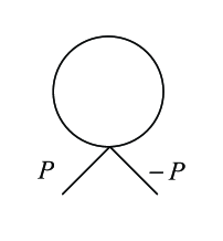
Figure 1: A one-loop single-propagator diagram.

We begin by considering a one-loop graph with only one internal propagator, as the one shown in figure 1. This particular graph contributes at first order to the self-energy in the $\lambda\phi^{4}$ theory. The actual number of external legs of the graph is unimportant, since we are only interested in the Matsubara sum associated with the loop. Although we could have considered this graph as the simplest case of the generic one-loop graph considered in section V, we prefer to analyze it separately, since the proof given in section V applies more naturally to the case of two or more internal propagators.

According to (4) the $D$-function for the graph of figure 1 is simply given by

$$D(p,E,T)=(2E)\,T\sum\limits_{n=-\infty}^{+\infty}\frac{1}{(2\pi Tn)^{2}+E^{2}}.$$ (11)

The sum above can be computed in a variety of ways and the result is well knownbooks-on-FTQFT . One obtains

$$D(p,E,T)=1+2n(E),$$ (12)

where $n(E)=\left(e^{\beta E}-1\right)^{-1}$ is the Bose-Einstein thermal occupation factor. The zero-temperature $D$-function, $D_{0}(\omega,E)$ can be computed directly from its definition,

$$D_{0}(\omega,E)=(2E)\int\limits_{-\infty}^{\infty}{\frac{{dk_{0}}}{{2\pi}}}\frac{1}{{k_{0}^{2}+E^{2}}},$$ (13)

or simply by taking the limit $T\to 0$ of $D(p,E,T)$ in (12). The result is

$$D_{0}(\omega,E)=1.$$ (14)

Since a constant function is unchanged by the reflection operator $\mathcal{S}_{E}$ defined by

$$\mathcal{S}_{E}f(E):=f(-E),$$ (15)

where $f$ is any regular function in the variable $E$, we certainly have the identity

$$D(p,E,T)=\big{[}1+n(E)(1+\mathcal{S}_{E})\big{]}D_{0}(p,E),$$ (16)

which proves that the thermal operator representation given by (7) and (8) does hold for the simple graph we are considering.

IV The two-vertex diagram

IV.1 Calculation

The Matsubara sum for the two-vertex diagram with $I$ internal propagators shown in figure 2 is most conveniently calculated using the Saclay methodsaclay-method , which we now briefly review.

Let $K:=(k,\mathbf{k})$ be the Euclidean 4-momentum vector associated with a given internal line; $k$ is a Matsubara frequency to be summed over.

Then each scalar propagator,

$$\Delta(K):=\frac{1}{K^{2}+m^{2}}=\frac{1}{k^{2}+E^{2}}:=\Delta(k,E),$$ (17)

where $E:=E_{\mathbf{k}}=\sqrt{\mathbf{k}^{2}+m^{2}}$, is represented as

$$\Delta(k,E)=\int_{0}^{\beta}d\tau\,e^{ik\tau}\Delta(\tau,E),$$ (18)

where $\beta=1/T$, as usual. The mixed propagator $\Delta(\tau,E)$, $0\leq\tau\leq\beta$, is given by

$$\Delta(\tau,E)=\frac{1}{2E}\left[\left(1+n(E)\right)e^{-E\tau}+n(E)e^{E\tau}\right],$$ (19)

where $n(E)=\left(e^{\beta E}-1\right)^{-1}$. For our purposes, it will be convenient to use the following representations for the mixed propagator (19):

$$\Delta(\tau,E) = \frac{1}{2E}\left[1+n(E)(1+\mathcal{S}_{E})\right]e^{-E\tau},$$ (20)

$$= \frac{n(E)e^{\beta E}}{2E}\left[1+e^{-\beta E}\mathcal{S}_{E}\right]e^{-E\tau},$$ (21)

where $\mathcal{S}_{E}$ is the reflection operator defined in (15). Substituting the representation (20) back into (18) and using the fact that the operator $(1/2E)[1+n(E)(1+\mathcal{S}_{E})]$ is linear, we obtain the following equivalent Saclay representation for the scalar propagator:

$$\Delta(k,E)=\frac{1}{2E}\left[1+n(E)(1+\mathcal{S}_{E})\right]\int_{0}^{\beta}d\tau\,e^{(ik-E)\tau}.$$ (22)

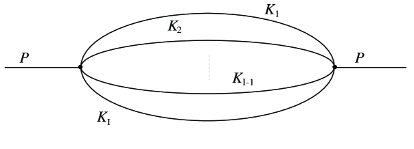
Figure 2: A two-vertex diagram with $I$ internal lines.

Consider now the two-vertex diagram with $I$ internal lines of figure 2. Let $P=(p,\mathbf{p})$ its external (incoming) 4-momentum (note that here $p$ stands for a single Euclidean energy variable) and let $K_{j}=(k_{j}=2\pi Tn_{j},\mathbf{k}_{j}),j=1,\ldots,I$, be the 4-momenta of the internal lines, flowing from the left to the right vertex. The Matsubara $D$-function corresponding to this graph is given by

$$\begin{split}D(p,{E},T)=&\gamma_{E}\,T^{I-1}\sum_{n_{1},n_{2},\dots,n_{I}}\prod_{j=1}^{I}\Delta(k_{j},E_{j})\delta_{k_{1}+\cdots+k_{I}\!,p},\end{split}$$ (23)

where the delta function is a Kronecker delta enforcing conservation of energy at both vertices, $\sum_{j=1}^{I}k_{j}=p$, and $\gamma_{E}$ was defined in (5).

Now, because the variables $p$ and $k_{j}$ are quantized in units of $2\pi T$, the Kronecker delta in (23) can be represented as

$$\delta_{k_{1}+\cdots+k_{I}\!,p}=T\int_{0}^{\beta}d\tau e^{-i\tau\left(k_{1}+\cdots+k_{I}\!-p\right)},$$ (24)

so that the sums over the integers $n_{j}$ decouple:

$$D(p,{E},T)=\gamma_{E}\,T^{I}\int_{0}^{\beta}d\tau e^{ip\tau}\prod_{j=1}^{I}\left[\sum_{n_{j}}\Delta(k_{j},E_{j})e^{-i\tau k_{j}}\right].$$ (25)

Using now the Saclay representation (22) for each propagator $\Delta(k_{j},E_{j})$ (with integration variable $\tau_{j}$) we find

$$\begin{split}D(p,{E},T)=&\;T^{I}\prod_{j=1}^{I}\left[1+n(E_{j})(1+\mathcal{S}_{E_{j}})\right]\\ &\times\int_{0}^{\beta}d\tau e^{ip\tau}\prod_{j=1}^{I}\left[\int_{0}^{\beta}d\tau_{j}\,e^{-E\tau_{j}}\sum_{n_{j}}e^{i(\tau_{j}-\tau)k_{j}}\right].\end{split}$$ (26)

But

$$T\sum_{n_{j}}e^{i(\tau_{j}-\tau)k_{j}} = \sum_{n}\delta(\tau_{j}-\tau+n\beta)$$ (27)

$$= \delta(\tau_{j}-\tau),\quad\text{for }0<\tau_{j},\tau<\beta,$$

so that the final result for the Matsubara $D$-function for the graph of figure 2 is:

$$D(p,{E},T) = \prod_{j=1}^{I}\left[1+n(E_{j})(1+\mathcal{S}_{j})\right]\int_{0}^{\beta}d\tau e^{(ip-E_{\rm tot})\tau}$$ (28)

$$= \prod_{j=1}^{I}\left[1+n(E_{j})(1+\mathcal{S}_{j})\right]\frac{e^{-\beta E_{\rm tot}}-1}{ip-E_{\rm tot}},$$

where $\mathcal{S}_{j}:=\mathcal{S}_{E_{j}}$, $E_{\rm tot}:=\sum_{j=1}^{I}E_{j}$ and we have used the fact that $\exp(i\beta p)\equiv 1$.

IV.2 Proof of the Thermal Operator Representation

We will now show that the result (28) can be put into the form (7), where the zero-temperature $D$-function for the graph of figure 2 is given by

$$D_{0}(p,{E})=-\left(\frac{1}{ip-E_{\rm tot}}-\frac{1}{ip+E_{\rm tot}}\right),$$ (29)

as can be easily be obtained from a calculation in the old-fashioned perturbation theory formalism. First, we observe that this function satisfies statement 3. In fact, since the only cut set of the two-vertex diagram is the set of all lines, we only need to show that the function (29) is annihilated by the operator

$$\mathcal{A}:=\prod_{j=1}^{I}(1+\mathcal{S}_{j}).$$ (30)

But since $\mathcal{S}_{x}$ is a reflection operator ($\mathcal{S}_{x}^{2}\equiv 1$) we have

$$\left[\prod_{j=1}^{I}(1+\mathcal{S}_{j})\right]\frac{1}{ip-E_{\rm tot}} = \left[\prod_{j=1}^{I}(1+\mathcal{S}_{j})\right]\left(\prod_{j=1}^{I}\mathcal{S}_{j}\frac{1}{ip+E_{\rm tot}}\right),$$ (31)

$$= \left[\prod_{j=1}^{I}(1+\mathcal{S}_{j})\right]\frac{1}{ip+E_{\rm tot}},$$

so that indeed $\mathcal{A}D_{0}(p,{E})\equiv 0$. Therefore it is enough to show that (7) holds with the thermal operator in the form (9). But this follows immediately from the following identity:

$$\left[\prod_{j=1}^{I}\left[1+n(E_{j})(1+\mathcal{S}_{j})\right]\right]\frac{e^{-\beta E_{\rm tot}}}{ip-E_{\rm tot}} = \left[\prod_{j=1}^{I}n(E_{j})e^{\beta E_{j}}\left[1+e^{-\beta E_{j}}\mathcal{S}_{j}\right]\right]\frac{e^{-\beta E_{\rm tot}}}{ip-E_{\rm tot}}$$

$$= \left[\prod_{j=1}^{I}n(E_{j})e^{\beta E_{j}}\left[1+e^{-\beta E_{j}}\mathcal{S}_{j}\right]e^{-\beta E_{j}}\mathcal{S}_{j}\right]\frac{1}{ip+E_{\rm tot}}$$

$$= \left[\prod_{j=1}^{I}\left[1+n(E_{j})(1+\mathcal{S}_{j})\right]\right]\frac{1}{ip+E_{\rm tot}},$$

where we have used the property $\left(e^{-\beta E_{j}}\mathcal{S}_{j}\right)^{2}\equiv 1$.

V The one-loop diagram

V.1 Calculation

The calculation of the Matsubara sum for the one-loop diagram with $I$ vertices and $I$ internal propagators shown in figure 3 is most conveniently done using the standard contour integration methodbooks-on-FTQFT . If a meromorphic function $f$ has no singularities along the imaginary axis and $k$ stands for the Matsubara frequency $k=2\pi Tn$, then

$$T\sum_{n=-\infty}^{\infty}f(ik)=\frac{1}{2\pi i}\oint_{C}f(z)n(z)dz,$$ (32)

where $n(z)=\left(e^{\beta z}-1\right)^{-1}$ and $C$ is the positive contour that runs vertically upwards the complex $z$-plane, infinitesimally to the right of the imaginary axis, from $\varepsilon-i\infty$ to $\varepsilon+i\infty$, and then comes back vertically and infinitesimally to the left of the imaginary axis, from $-\varepsilon+i\infty$ to $-\varepsilon-i\infty$, with $\varepsilon=0^{+}$.

If $|n(z)f(z)|$ goes fast enough to zero when $|z|$ goes to infinity we can change the contour of integration to two negatively oriented semicircumferences, one on each side of the imaginary axis, with radii tending to infinity. Thus, by Cauchy’s integral theorem,

$$T\sum_{n=-\infty}^{\infty}f(ik)=-\sum_{l}{\rm Res}_{z=z_{l}}[f(z)n(z)],$$ (33)

where $z_{l}$ are the poles of the function $f(z)$.

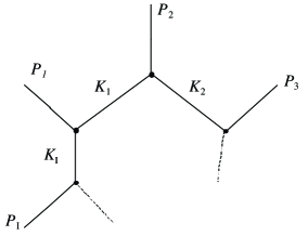
Figure 3: A one-loop diagram with $I$ vertices.

Consider now the one loop graph of figure 3. Let $P_{i}=(p_{i},\mathbf{p}_{i})$ be the external incoming momenta at each vertex. Letting $k=2\pi nT$ be the Matsubara frequency of line $1$, the Matsubara $D$-function in this case can be reduced to the form

$$D(p,E,T)=\gamma_{E}\,T\sum_{n}\Delta(k,E_{1})\Delta(k+p_{2},E_{2})\cdots\Delta(k+\sum_{j=2}^{I}p_{j},E_{I}),$$ (34)

where the energies $E_{i}$ are defined as before. Introducing a new set of variables $u_{j}:=\sum_{l=1}^{j}p_{l}-p_{1}\;\;(j=2,\ldots,I)$ and letting $u_{1}:=0$, we can write (34) as

$$D(p,E,T)=\gamma_{E}\,T\sum_{n}\prod_{j=1}^{I}\Delta(k+u_{j},E_{j}).$$ (35)

Next using the identity

$$\frac{1}{k^{2}+E^{2}}=-\frac{1}{2E}\left(\frac{-1}{ik+E}+\frac{1}{ik-E}\right)=-\frac{1}{2E}\sum_{\sigma=\pm 1}\frac{\sigma}{ik-\sigma E},$$ (36)

we get

$$\begin{split}D(p,E,T)=&(-1)^{I}\,T\sum_{n}\left\{\prod_{j=1}^{I}\left[\sum_{\sigma_{j}=\pm 1}\frac{\sigma_{j}}{ik+iu_{j}-\sigma_{j}E_{j}}\right]\right\},\\ =&(-1)^{I}\,T\sum_{n}\left\{\sum_{\sigma}\prod_{j=1}^{I}\frac{\sigma_{j}}{ik+iu_{j}-\sigma_{j}E_{j}}\right\},\end{split}$$ (37)

where now $\sigma:=\{\sigma_{1},\sigma_{2},\dots,\sigma_{I}\}$. If the function between brackets in (37) is called $f(ik)$, then we see that the poles of $f(z)$ are located at $z_{l}=-iu_{l}+\sigma_{l}E_{l}$, so that the application of (33) gives us

$$D(p,E,T)=(-1)^{I+1}\,\sum_{\sigma}\sum_{l=1}^{I}n(\sigma_{l}E_{l})\sigma_{l}\prod_{j\not{=}l}^{I}\frac{\sigma_{j}}{i(u_{j}-u_{l})+\sigma_{l}E_{l}-\sigma_{j}E_{j}}.$$ (38)

In order to express the result for the $D$-function in terms of Bose-Einstein factors of positive argument only, we will perform the summation over $\sigma_{l}$ explicitly. Introducing the notation $\sigma_{\!\!\not{\;l}}:=(\sigma_{1},\dots,\sigma_{l-1},\sigma_{l+1},\dots,\sigma_{I})$ and using the identity $n(-E_{l})=-(1+n(E_{l}))$ we find

$$\begin{split}D(p,&E,T)=(-1)^{I+1}\sum_{l=1}^{I}\sum_{\sigma_{\!\!\not{\;l}}}\left\{\prod_{j\neq l}^{I}\frac{\sigma_{j}}{i(u_{j}-u_{l})-E_{l}-\sigma_{j}E_{j}}+\right.\\ &\phantom{xxxxxxxxxxxxxxxxxxxx}\left.+n(E_{l})\left[\prod_{j\neq l}^{I}\frac{\sigma_{j}}{i(u_{j}-u_{l})-E_{l}-\sigma_{j}E_{j}}+\prod_{j\neq l}^{I}\frac{\sigma_{j}}{i(u_{j}-u_{l})+E_{l}-\sigma_{j}E_{j}}\right]\right\}.\end{split}$$ (39)

In terms of the auxiliary function

$$\begin{split}d_{l}(p,E):=&\sum_{\sigma_{\!\!\not{\;l}}}\prod_{j\neq l}^{I}\frac{\sigma_{j}}{i(u_{j}-u_{l})-E_{l}-\sigma_{j}E_{j}}\\ =&\prod_{j\neq l}^{I}\sum_{\sigma_{j}}\frac{\sigma_{j}}{i(u_{j}-u_{l})-E_{l}-\sigma_{j}E_{j}},\end{split}$$ (40)

and the reflection operator, $\mathcal{S}_{i}:=\mathcal{S}_{E_{i}}$, defined in (15) we have

$$D(p,E,T)=(-1)^{I+1}\sum_{l=1}^{I}\left[d_{l}(p,E)+n(E_{l})(1+\mathcal{S}_{E_{l}})d_{l}(p,E)\right].$$ (41)

V.2 Proof of the Thermal Operator Representation

We shall prove now that the $D$-function (41) for the one-loop graph of figure 3 can be written in the form (7), as

$$D(p,E,T)=\left[1+\sum_{j=1}^{I}n(E_{j})(1+\mathcal{S}_{j})\right]D_{0}(p,E),$$ (42)

with

$$D_{0}(p,E)=(-1)^{I+1}\sum_{l=1}^{I}d_{l}(p,E).$$ (43)

Since the graph of figure 3 gets disconnected if two or more lines are snipped, the thermal operator has terms no higher than linear in the Bose-Einstein factors $n(E)$. But equation (42) will reduce to eqn. (41) if the operator $(1+\mathcal{S}_{j})$ annihilates the auxiliary function $d_{l}(p,E)$ when $j\neq l$. This is indeed the case: from equation (40) we see that when $j\neq l$

$$\begin{split}d_{l}(p,E)=&\sum_{\sigma_{j}}\frac{\sigma_{j}}{i(u_{j}-u_{l})-E_{l}-\sigma_{j}E_{j}}\prod_{k\neq l\!,\,j}^{I}\sum_{\sigma_{k}}\frac{\sigma_{k}}{i(u_{k}-u_{l})-E_{l}-\sigma_{k}E_{k}},\\ =&\sum_{\sigma_{j}}\frac{-\sigma_{j}}{i(u_{j}-u_{l})-E_{l}+\sigma_{j}E_{j}}\prod_{k\neq l\!,\,j}^{I}\sum_{\sigma_{k}}\frac{\sigma_{k}}{i(u_{k}-u_{l})-E_{l}-\sigma_{k}E_{k}}\\ =&-\mathcal{S}_{j}d_{l}(p,E),\end{split}$$ (44)

which means that

$$(1+\mathcal{S}_{j})d_{l}(p,E)\equiv 0,\quad\text{if }j\neq l.$$ (45)

Statement 1 is then valid for the one-loop graph of figure 3.

Furthermore, statement 3 is also true for this graph. In fact, any cut set will at least contain two lines, say lines $i$ and $j$. But then

$$(1+\mathcal{S}_{i})(1+\mathcal{S}_{j})d_{l}(p,E)\equiv 0,$$ (46)

since, for any given $l$, either $i$ or $j$ will be different from $l$ (since $i\neq j$), leading to a vanishing contribution because of (45).

VI Further evidence and conclusions

One piece of evidence in favor of the general validity of the representation (7) is provided by a comparison with a well known result of thermal field theory, first formulated by Weldonweldon , concerning the interpretation of the imaginary part of the retarded self-energy $\Pi_{R}$ in terms of the direct and inverse decay rates of a particle propagating in the thermal medium. A well-known result of quantum statistical mechanicsBaym and Mermin is that the full retarded self-energy $\Pi_{R}$ can be obtained from the Euclidean self-energy $\Pi_{\beta}$ by analytic continuation as

$$\Pi_{R}(\omega,{\mathbf{p}})=-\Pi_{\beta}(i(\omega+i\varepsilon),{\mathbf{p}}),$$ (47)

where $\omega$ stands for a real continuous variable. In the context of perturbative quantum field theory, the imaginary part of $\Pi_{R}$ is given in the form of integrals over phase space of amplitudes squared, weighted by certain statistical factors that account for the possibility of particle absorption from the medium or particle emission into the mediumweldon . For example, for the one-loop 2-vertex diagram corresponding to figure 4 in the appendix that follows, the result for the imaginary part of the retarded self- energy is (we have set $g\equiv 1$)

$$\operatorname{Im}\Pi_{R}(\omega,{\mathbf{p}}) = -\pi\int{\frac{{d^{3}k}}{{(2\pi)^{3}}}\frac{1}{{4E_{1}E_{2}}}}\Big{[}{(1+n_{1}+n_{2})}\big{(}{\delta(\omega-E_{1}-E_{2})-\delta(\omega+E_{1}+E_{2})}\big{)}$$ (48)

$$\phantom{xxxxxxxxxxxxxxxx}{-(n_{1}-n_{2})\big{(}{\delta(\omega-E_{1}+E_{2})-\delta(\omega+E_{1}-E_{2})}\big{)}}\Big{]}.$$

where $n_{i}\equiv n(E_{i})$. But from the general form (3) for a diagram in the Euclidean formalism, it is clear that the imaginary part of the analytically continued diagram is determined by the analytic continuation of its $D$-function. The general validity of our main representation in the form (7) would imply that the latter is in turn completely determined in terms of the analytic continuation of the zero-temperature $D$-function, $D_{0}$, since the thermal operator $\hat{O}$ is real and does not involve the external momenta.

For the particular simple diagram we are considering, which is actually a special case of the general 2-vertex graph considered in section IV, the Thermal Operator Representation has been proven to hold. Hence

$$\operatorname{Im}D\left({i(\omega+i\varepsilon),E_{1},E_{2},T}\right)=\hat{O}\left({E_{1},E_{2},T}\right)\operatorname{Im}D_{0}\left({i(\omega+i\varepsilon),E_{1},E_{2}}\right).$$ (49)

The last imaginary part could in principle be obtained from the standard cutting rules that apply in zero-temperature field theory, without having to compute $D_{0}$ itself. In this case, however, we have the closed result (29) for $D_{0}$, which allows us to compute directly

$$\operatorname{Im}D_{0}\left({i(\omega+i\varepsilon),E_{1},E_{2}}\right) = \operatorname{Im}\left[{\frac{1}{{\omega+E_{1}+E_{2}+i\varepsilon}}-\frac{1}{{\omega-E_{1}-E_{2}+i\varepsilon}}}\right]$$ (50)

$$= -\pi\left[{\delta(\omega+E_{1}+E_{2})-\delta(\omega-E_{1}-E_{2})}\right].$$

Now in this case the thermal operator is given by

$$\hat{O}\left({E_{1},E_{2},T}\right)=1+n_{1}(1+\mathcal{S}_{1})+n_{2}(1+\mathcal{S}_{2})=1+n_{1}+n_{2}+n_{1}\mathcal{S}_{1}+n_{2}\mathcal{S}_{2}.$$ (51)

Since

$$n_{1}\mathcal{S}_{1}\left[{\delta(\omega+E_{1}+E_{2})-\delta(\omega-E_{1}-E_{2})}\right]=n_{1}\left[{\delta(\omega-E_{1}+E_{2})-\delta(\omega+E_{1}-E_{2})}\right],$$

etc., we readily obtain

$$\hat{O}\operatorname{Im}D_{0} = \pi\Big{[}{(1+n_{1}+n_{2})}\big{(}{\delta(\omega-E_{1}-E_{2})-\delta(\omega+E_{1}+E_{2})}\big{)}$$ (52)

$$\quad{-(n_{1}-n_{2})\big{(}{\delta(\omega-E_{1}+E_{2})-\delta(\omega+E_{1}-E_{2})}\big{)}}\Big{]},$$

thereby reproducing (48), with all the correct signs and thermal factors.

In this paper we have restricted our attention to some simple diagrams in the finite-temperature imaginary-time formalism for a scalar relativistic field theory. We have shown that the full result of performing the Matsubara sum associated to any given Feynman graph can be obtained from its zero-temperature counterpart, by means of a simple linear operator. Given the general form (8) of the thermal operator, which can be readily and naturally extrapolated to diagrams of arbitrary topologies, it is not at all implausible that the representation (7) be actually valid in complete generality. This generalization remains an open problem however, and work in this direction is in progress.

An analysis similar to the one presented here should apply in a theory containing fermions; the algebra will be slightly more complicated because of the spin structure. We have deferred this analysis, as well as the extension of our results to gauge theories, until we have been able to prove or disprove that the Thermal Operator Representation put forward in this paper does indeed hold for an arbitrary loop graph in a scalar field theory.

VII Acknowledgement

The authors would like to thank C. Dib and I. Schmidt for suggestions, O. Orellana for interesting insights, and the first referee for helpful criticisms and comments to the original version of this work. This work was supported by CONICYT, under grant Fondecyt 8000017. E.S. would also like to thank the Physics Department of Universidad Santa María for its hospitality and the partial financial support of the Millennium Scientific Nucleus ICM P99-135F.

VIII Appendix

VIII.1 The OFPT-rules

The rules originally put forward in reference DES-97 to write down an explicit expression for the Matsubara $D$-function corresponding to the general scalar graph considered in section II are given by the following statements (it might be useful to refer to figure 4 at this point):

• For each external line, characterized by a real Euclidean 4-vector $(p_{l},{\bf p}_{l})$, define its energy as $ip_{l}$. For each internal line define its energy as $E_{i}=({\bf k}_{i}^{2}+m_{i}^{2})^{1/2}$, where ${\bf k}_{i}$ is the 3-momentum carried by the line and $m_{i}$ is the mass of the propagating particle.

• Define a direction of time or energy flow (which we shall take conventionally from left to right) and consider all possible orderings of the vertices along this direction (see, e.g., Figs. 4.a and 4.b. For a graph with $n+1$ vertices there will be $(n+1)!$ such orderings).

• For each time-ordered graph generated in (b) consider, in addition to itself, all possible connected graphs that can be obtained by snipping any number of internal lines. Each line that is snipped becomes a pair of legs we shall call thermal legs. Attach a cross to their ends to distinguish them from the original external lines of the graph. Both legs of a given pair inherit the energy $E_{i}$ of the internal line that originated them. However, one leg must be oriented as incoming with energy $E_{i}$ and the other as outgoing with energy $E_{i}$. Both possible orientations have to be considered, each one generating a different diagram (see, e.g., Figs. 4.c and 4.d).

• For each graph in (c), define its total incoming energy, $E_{inc}$, as the sum of all incoming external energies plus the energies of all incoming thermal legs that join the diagram before their outgoing partner (e.g. as in Figs. 4.d and 4.f). Thermal leg pairs that satisfy this property shall be referred to as external, and those that do not as internal (e.g. as in Figs. 4.c and 4.e). Then, associate to this graph an expression equal to the product of the following factors:

  • draw a full vertical division (a “cut”) between each pair of consecutive time-ordered vertices (there are $n$ such cuts in a graph with $n+1$ vertices); for each cut include a factor

    $$\frac{1}{E_{inc}-E_{cut}}$$ (53)

    where $E_{cut}$ is the total energy of the intermediate state associated with the cut, defined as the sum of the energies of all the lines that cross the cut in question (as in zero-temperature time-ordered perturbation theory), plus the energies of all internal thermal pairs whose originating internal line would have crossed the cut.

  • include a thermal occupation factor $n_{i}\equiv n(E_{i})$ for each thermal pair (of energy $E_{i}$) in the diagram (if any).

  • include an overall factor of $(-1)^{n}$, where $n+1$ is the number of vertices.

• The integrand $D(p,E,T)$ in (3), i.e., the Matsubara $D$-function of the graph, is the sum of the expressions computed according to rule (d), over all the graphs in (c).

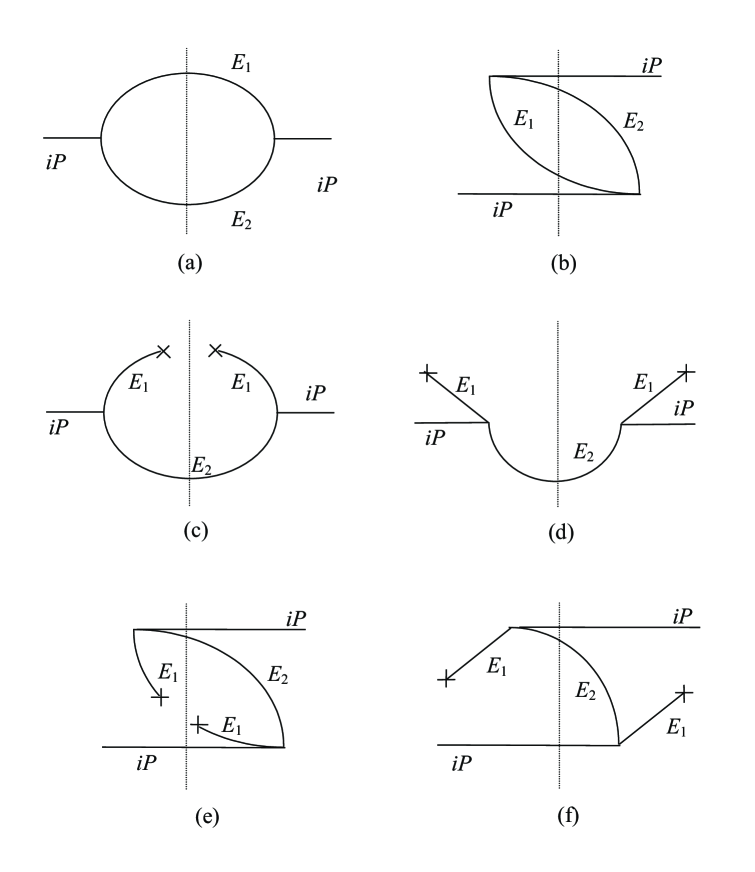
Figure 4: An example of the diagrams which appear in the OPFT-rules.

VIII.2 An algebraic approach to the OFPT-rules

Let us call $D_{R}(p,E,T)$ the expression for the $D$-function generated according to the OFPT-rules. A trivial check the OFPT-rules do satisfy is that they yield the known correct result in the limit $T\to 0$, keeping the external Euclidean energies $p$ fixed. In fact, in the limit $T\to 0$ all the thermal factors $n(E)$ vanish, so that according to the rules $D_{R}(p,E,0)$ is just given by all possible time ordered diagrams with no snipped lines, calculated according to rule (d) above. But this is precisely the result one would obtain calculating the $T=0$ Euclidean graph (with external momenta $(p_{l},\mathbf{p}_{l})$) using old-fashioned perturbation theoryOFPT . We have therefore:

$$D_{0}(p,E)=D_{R}(p,E,0),$$ (54)

where $D_{0}(p,E)$ is the $D$-function associated with the zero-temperature Euclidean Feynman graph. Hence, the rules hold at $T=0$.

At finite temperature, we get extra contributions according to rules (c) and (d) above. Now, instead of considering, as commanded by rule (c), all possible connected graphs that can be obtained by snipping any number of internal lines of a given “un-snipped” time-ordered graph, let us rather group the snipped diagrams according to which lines are snipped, regardless of the time-ordering. Take for instance all the diagrams which have only the $i$-th line snipped ($i$ is fixed). A set of this type is conformed, for instance, by the diagrams (c) to (f) of Fig.4. It follows directly from rule (d.1) that a diagram in which the snipped line forms an internal thermal leg pair (i.e., we have a “closed” snipping, as in Figs. 4.c and 4.e) has exactly the same mathematical weight as the zero-temperature “un-snipped” diagram, except of course for the extra thermal factor $n(E_{i})$. Thus the sum of all these diagrams, i.e., the diagrams that have only the $i$-th line snipped closed, adds up to $n(E_{i})D_{0}(p,E)$. On the other hand, if the snipped line forms an external thermal leg pair (i.e., we have a “open” snipping, as in Figs. 4.d and 4.f), we again have an extra thermal factor $n(E_{i})$, but now the rest of the expression differs from that for the “un-snipped” graph in the sign of the energy $E_{i}$. This is so because, for an open snipping, the energy $E_{i}$ moves from $E_{cut}$ to $E_{inc}$, as can be gathered from rule (d).

Let $x$ symbolize a variable, and let $\mathcal{S}_{x}$ be the operator that acts on functions of $x$, changing the sign of the argument $x$, according to:

$$\mathcal{S}_{x}f(x):=f(-x).$$

In terms of the reflection operator $\mathcal{S}_{x}$, we can write the sum of all the time-ordered diagrams with only the $i$-th line snipped open as

$$n(E_{i})\mathcal{S}_{i}D_{0}(p,E),$$

where we have written $\mathcal{S}_{i}:=\mathcal{S}_{E_{i}}$ to avoid cluttering the notation. So the full contributions of the diagrams in which only the $i$-th line is snipped can be written as

$$n(E_{i})\left(1+\mathcal{S}_{i}\right)D_{0}(p,E).$$

The analysis above can clearly be generalized to add up the contribution of the graphs with more than one snipped line. Taking into account that only connected graphs are allowed by the OFPT-rules (so that one is allowed to snip at most $L$ internal lines, where $L$ is the number of independent loops), we arrive at the following result:

Theorem 1.

The OFPT-rules admit the following mathematical representation:

$$D_{R}(p,E,T)=\hat{O}(E,T)D_{0}(p,E),$$ (55)

where $\hat{O}(E,T)$, the thermal operator, is given by

$$\begin{split}\hat{O}(E,T):=1+&\sum_{i=1}^{I}n(E_{i})(1+\mathcal{S}_{i})+\sideset{}{{}^{\prime}}{\sum}_{\langle i_{1},i_{2}\rangle}n(E_{i_{1}})n(E_{i_{2}})(1+\mathcal{S}_{i_{1}})(1+\mathcal{S}_{i_{2}})\\ +&\dots+\sideset{}{{}^{\prime}}{\sum}_{\langle i_{1},\dots,i_{L}\rangle}\prod_{l=1}^{L}n(E_{i_{l}})(1+\mathcal{S}_{i_{l}}).\end{split}$$ (56)

Here the indices $i_{1},i_{2},\ldots$ run from 1 to $I$ (the number of internal propagators) and the symbol $\langle i_{1},\dots,i_{k}\rangle$ stands for an unordered $k$-tuple with no repeated indices. The primes on the summation symbols imply that we are to exclude from the sums those tuples $\langle i_{1},\dots,i_{k}\rangle$ such that if we snip all the corresponding lines $i_{1},\dots,i_{k}$ then the graph becomes disconnected.

References

- (1) For a review of the early literature on the subject see, for example, N.P. Landsman and Ch.G. van Weert, Phys. Rep. 145, 141 (1987). For more modern introductions to the subject see, for instance, J. Kapusta, Finite-temperature field theory (Cambridge, 1993); M. Le Bellac, Thermal field theory (Cambridge, 1996); A. Das, Finite temperature field theory (World Scientific, 1997).
- (2) R. Balian and C. de Dominicus, Nucl. Phys. 16, 502 (1960); G. Baym and A.M. Sessler, Phys. Rev. 131, 2345 (1963); I.E. Dzyaloshinski, Sov. Phys. JEPT 15, 778 (1962); R.P. Pisarski, Nucl. Phys. B309, 476 (1988); E. Braaten and R.D. Pisarski, Nucl. Phys. B337, 569 (1990).
- (3) F. Guerin, Phys. Rev. D49, 4182 (1994).
- (4) C. Dib, O. Espinosa and I. Schmidt,Phys. Lett. B402, 147 (1997).
- (5) J. Frenkel and J.C. Taylor, Nucl. Phys. B374, 156 (1992); F.T. Brandt and J. Frenkel, Phys. Rev. D56, 2453 (1997).
- (6) F.T. Brandt, A. Das, J. Frenkel and A.J. da Silva, Phys. Rev. D59, 065004 (1999).
- (7) R. Kobes, Phys. Rev. D42, 562 (1990); Phys. Rev. Lett. 67, 1384 (1991); T.S. Evans, Phys. Lett. B249, 286 (1990); Phys. Lett. B252, 108 (1990); Nucl. Phys. B374, 340 (1992); P. Aurenche and T. Becherrawy, Nucl. Phys B379, 259 (1992); R. Baier and A. Niégawa, Phys. Rev D49, 4107 (1994); M.A. van Eijck, R. Kobes and Ch. G. van Weert, Phys. Rev. D50, 4097 (1994).
- (8) R.L. Kobes and G.W. Semenoff, Nucl. Phys B260, 714 (1985); B272, 329 (1986); R. Kobes, Phys. Rev. D43, 1269 (1991); P.V. Landshoff, Phys. Lett. B386, 291 (1996); P. F. Bedaque, A. Das, and S. Naik, Mod. Phys. Lett. A12, 2481 (1997); A. Niégawa, Phys. Rev. D57, 1379 (1998); M.E. Carrington, Hou Defu, and R. Kobes, Phys. Rev. D67, 025021 (2003);
- (9) See, for example, S. Weinberg, Phys. Rev. 150, 1313 (1966); or S.S. Schweber, An Introduction to Relativistic Quantum Field Theory, Harper and Row, New York, 1961.
- (10) H.A. Weldon Phys. Rev. D28, 2007 (1983).
- (11) G. Baym and N.D. Mermin, Jour. Math. Phys. 2, 232 (1961).