FT-UM-TH-03-02

FIS-UM-03-10

hep-ph/0304297

KamLAND, solar antineutrinos and the solar magnetic field

Bhag C. Chauhan^a, João Pulido^a, E. Torrente-Lujan^b
a Centro de Física das Interacções Fundamentais (CFIF)
Departamento de Física, Instituto Superior Técnico
Av. Rovisco Pais, P-1049-001 Lisboa, Portugal
^b Departamento de Fisica, Grupo de Fisica Teorica,
Universidad de Murcia, Murcia, Spain

In this work the possibility of detecting solar electron antineutrinos produced by a solar core magnetic field from the KamLAND recent observations is investigated. We find a scaling of the antineutrino probability with respect to the magnetic field profile in the sense that the same probability function can be reproduced by any profile with a suitable peak field value. In this way the solar electron antineutrino spectrum can be unambiguosly predicted. We use this scaling and the negative results indicated by the KamLAND experiment to obtain upper bounds on the solar electron antineutrino flux. We get $\phi_{\bar{\nu}}<3.8\times 10^{-3}\phi(^{8}B)$ at 95% CL. For 90% CL this becomes $\phi_{\bar{\nu}}<3.4\times 10^{-3}\phi(^{8}B)$, an improvement by a factor of 3-5 with respect to existing bounds. These limits are independent of the detailed structure of the magnetic field in the solar interior. We also derive upper bounds on the peak field value which are uniquely determined for a fixed solar field profile. In the most efficient antineutrino producing case, we get (95% CL) an upper limit on the product of the neutrino magnetic moment by the solar field $\mu B<2.8\times 10^{-19}$ MeV or $B_{0}\leq 4.9\times 10^{7}G$ for $\mu_{\nu}=10^{-12}\mu_{B}$.

1 Introduction

The recent results from the KamLAND experiment [1] have asserted that the large mixing angle solution (LMA) is the dominant one for the 34 year old solar neutrino problem SNP [2]. Although neutrinos were known, before KamLAND data, to oscillate [3, 4], it was not clear if neutrino oscillations were the major effect underlying the solar neutrino deficit or whether they played any role at all. It had been clear however that this deficit had to rely on ’non-standard’ neutrino properties. To this end, the spin flavor precession (SFP) [5, 6, 7], based on the interaction of the neutrino magnetic moment with the solar magnetic field was, second to oscillations, the most attractive scenario [8].

SFP, although certainly not playing the major role in the solar neutrino deficit, may still be present as a subdominant process, provided neutrinos have a sizeable transition magnetic moment. Its signature will be the appearance of solar antineutrinos [6, 9, 10] which result from the combined effect of the vacuum mixing angle $\theta$ and the transition magnetic moment $\mu_{\nu}$ converting neutrinos into antineutrinos of a different flavor. This can be schematically shown as

$${\nu_{e}}_{L}\rightarrow{\nu_{\mu_{L}}}\rightarrow{\bar{\nu}_{e_{R}}},$$ (1)

$${\nu_{e}}_{L}\rightarrow{\bar{\nu}_{\mu_{R}}}\rightarrow{\bar{\nu}_{e_{R}}}$$ (2)

with oscillations acting first and SFP second in sequence (1) and in reverse order in sequence (2). Oscillations and SFP can either take place in the same spatial region, or be spatially separated. Independently of their origin, antineutrinos with energies above 1.8 MeV can be detected in KamLAND via the observation of positrons from the inverse $\beta$-decay reaction $\bar{\nu}_{e}+p\rightarrow n+e^{+}$ and must all be originated from ${}^{8}B$ neutrinos.

The purpose of this work is to relate the solar magnetic field profile to the solar antineutrino event rate in KamLAND which is a component of the total positron event rate in the reaction above. In a previous paper [11] the question of what can be learned about the strength and coordinate dependence of the solar magnetic field in relation to the current upper limits on the solar $\bar{\nu}_{e}$ flux was addressed. The system of equations describing neutrino evolution in the sun was solved analytically in perturbation theory for small $\mu_{\nu}{B}$, the product of the neutrino magnetic moment by the solar field. The three oscillation scenarios with the best fits were considered, namely LMA, LOW and vacuum solutions. In particular for LMA it was found that the antineutrino probability depends only on the magnitude of the magnetic field in the neutrino production zone. Neutrinos were, in the approximation used, considered to be all produced at the same point ($x=0.05R_{S}$), where ${}^{8}B$ neutrino production is peaked. In this work we will consider the more realistic case of a convolution of the production distribution spectrum with the field profile in that region. It will be seen that this convolution leads to an insensitiveness of the antineutrino probability with respect to the solar magnetic field profile, in the sense that different profiles can correspond to the same probability function, provided the peak field values are conveniently scaled. As a consequence, an upper bound on the solar antineutrino flux can be derived which is independent of the field profile and the energy spectrum of this flux will also be seen to be profile independent.

Up to now, in their published data from a 145 day run, the KamLAND [1] experiment has observed a total antineutrino flux compatible with the expectations coming from the nearby nuclear reactors. Given this fact, and evaluating the positron event rate for the above reaction for different solar field profiles, we will derive upper bounds for the peak field value in each profile. In our study we will assume the astrophysical upper bounds on the neutrino magnetic moment $\mu_{\nu}<(1-3)\times 10^{-12}\mu_{B}$ [12] to be all satisfied and take $\mu_{\nu}=10^{-12}\mu_{B}$.

Upper limits on the solar antineutrino flux, the intrinsic magnetic moment and the magnetic field at the bottom of the convective zone were recently obtained [10] from the published KamLAND data. Here we address however a different antineutrino production model where the magnetic field at the solar core is the relevant one.

2 The solar antineutrino probability

We start with the probability that a ${\nu_{e}}_{L}$ produced inside the sun will reach the earth as a $\bar{\nu}_{e_{R}}$

$$P(\nu_{e_{L}}\rightarrow\bar{\nu}_{e_{R}})=P(\nu_{e_{L}}\rightarrow\bar{\nu}_{\mu_{R}};R_{S})\times P(\bar{\nu}_{\mu_{R}}\rightarrow\bar{\nu}_{e_{R}};R_{es})$$ (3)

in which the first term is the SFP probability, $R_{S}$ is the solar radius and the second term is given by the well known formula for vacuum oscillations

$$P(\bar{\nu}_{\mu_{R}}\rightarrow\bar{\nu}_{e_{R}};R_{es})={\sin}^{2}2\theta~{}~{}{\sin}^{2}\!\left(\frac{\Delta m^{2}}{4E}R_{es}\right)=\frac{1}{2}.$$ (4)

Here $R_{es}$ is the distance between the sun and the earth and the rest of the notation is standard. Since $1.8MeV<E<15MeV$ and, for LMA, $\Delta m^{2}=6.9\times 10^{-5}eV^{2}$, $\sin^{2}2\theta=1$ [1], we take the $\bar{\nu}_{\mu_{R}}\rightarrow\bar{\nu}_{e_{R}}$ vacuum oscillations to be in the averaging regime.

The SFP amplitude in perturbation theory for small $\mu B$ is [11]

$$A(\nu_{e_{L}}\rightarrow\bar{\nu}_{\mu_{R}})=\frac{\mu B(r_{i})\sin^{2}\theta(r_{i})}{g^{{}^{\prime}}_{2}(r_{i})}.$$ (5)

A key observation is that the antineutrino appearance probability is dependent on the production point of its parent neutrino so that the overall antineutrino probability is

$$P(\nu_{e_{L}}\rightarrow\bar{\nu}_{e_{R}})=\frac{1}{2}\int|A(\nu_{e_{L}}\rightarrow\bar{\nu}_{\mu_{R}})|^{2}f_{B}(r_{i})dr_{i}$$ (6)

where $f_{B}$ represents the neutrino production distribution function for Boron neutrinos [13] and the integral extends over the whole production region. As shall be seen, owing to this integration, the energy shape of probability (6) is largely insensitive to the magnetic field profile.

The positron event rate in the KamLAND experiment originated from solar antineutrinos is then

$$S=Q_{0}\int_{E_{e}^{0}}^{\infty}dE_{e}\int_{E_{m}}^{E_{M}}\epsilon(E^{{}^{\prime}}_{e})R(E_{e},E^{{}^{\prime}}_{e})\phi_{\bar{\nu}}(E)\sigma(E)dE.$$ (7)

In this expression $Q_{0}$ is a normalization factor which takes into account the number of atoms of the detector and its live time exposure [1] and $E$ is the antineutrino energy, related to the physical positron energy by $E^{{}^{\prime}}_{e}=E-(m_{N}-m_{P})$ to zero order in $1/M$, the nucleon mass. We thus have $E_{m}=1.804MeV$, while the KamLAND energy cut is $E_{e}^{0}=2.6MeV$. The functions $\epsilon$ and $R$ denote the detector efficiency and the Gaussian energy resolution function of the detector

$$R(E_{e},E^{{}^{\prime}}_{e})=\frac{1}{s\sqrt{2\pi}}\exp\left[\frac{-(E_{e}-E^{{}^{\prime}}_{e})^{2}}{2s^{2}}\right].$$ (8)

In our analysis we use for the energy resolution in the prompt positron detection the expression $s(E_{e})=0.0062+0.065\surd E_{e}$ with all energy units in MeV. This is obtained from the raw calibration data presented in Ref.[14]. Moreover, we assume a 408 ton fiducial mass and the detection efficiency is taken independent of the energy [14], $\epsilon\simeq 80\%$, which amounts to 162 ton. yr of antineutrino data. The antineutrino cross section $\sigma(E)$ was taken from ref.[15] and we considered energy bins of size $E_{e}=0.425\ MeV$ in the KamLAND observation range $(2.6-8.125)~{}MeV$ [1]. The antineutrino spectral flux $\phi_{\bar{\nu}}(E)$ in eq. 7 can be written as $\phi_{\bar{\nu}}(E)=\phi_{\bar{\nu}}^{0}\times f(E)$ where $\phi_{\bar{\nu}}^{0}$ is the total antineutrino flux and $f(E)$ is some function of the energy normalized to one. The function $\phi_{\bar{\nu}}(E)$ is on the other hand a simple product of the Boron neutrino spectral flux $\phi_{B}(E)$ which can be found in Bahcall’s homepage [13] and the antineutrino appearance probability we obtained above: $\phi_{\bar{\nu}}(E)=\phi_{B}(E)\times P(E)$. The almost insensitivity of the shape of $P(E)$ to the shape of the magnetic field profile is thus necessarily reflected in $\phi_{\bar{\nu}}(E)$. The only significant dependence appears on the normalization constant $\phi_{\bar{\nu}}^{0}$ which is essentially proportional to the square of the magnetic field at the solar core. We make use of this behavior to obtain, for each given profile, upper limits on the core magnetic field, the total antineutrino flux and the intrinsic neutrino magnetic moment.

As mentioned above, for the LMA solution only the solar field profile in the neutrino production region [11] can affect the antineutrino flux. Hence we will discuss three profiles which span a whole spectrum of possibilities at this region. We study from a vanishing field (profile 1) to a maximum field at the solar center, with, in this second case, either a fast decreasing field intensity (profile 2) or a nearly flat one (profile 3) in the solar core (see fig. 1, lower panel). Thus, we consider respectively the following three profiles

Profile 1

$$B(r)=B_{0}[\cosh(9r)-1]~{}~{},~{}~{}|r|\leq r_{c}$$ (9)

$$B(r)=B_{0}/\cosh[25(r-r_{R})]~{}~{},~{}~{}|r|>r_{c},$$ (10)

with $r_{c}=0.08$, $r_{R}=0.16$,

Profile 2

$$B(r)=B_{0}/\cosh(15r)~{}~{},~{}~{}|r|\geq 0,$$ (11)

Profile 3

$$B(r)=B_{0}[1-(r/r_{c})^{2}]~{}~{},~{}~{}|r|\leq r_{c},$$ (12)

with $r_{c}=0.713$.

We also show in fig. 1 (upper panel) the ${}^{8}B$ production distribution spectrum, so that a comparison between the strength of the field and the production intensity can be directly made.

The antineutrino production probabilities as a function of energy for each of these profiles are given in fig. 2. In the first panel, the values of the peak field are chosen so as to produce a fixed number of events. In this case the probability curves differ only slightly in their shapes while their normalizations are the same. The curves are in any case similar to the SFP survival probability ones [16] in the same energy range. In the second panel of fig. 2 the antineutrino probabilities for a common value of the peak field and these three different profiles are shown. It is hence apparent from these two graphs how the distribution of the magnetic field intensity is determinant for the magnitude of the antineutrino probability, but not for its shape. One important reason for this behavior is that we have integrated the antineutrino probability over the Boron production region.

3 Results and discussion

The antineutrino signal for any magnetic field profile $B(r)$ can be written, taking into account the previous formulas and the near invariance of the probability shape (see fig. 2), as

$$S_{\overline{\nu}}[{B(r)}] = \alpha S_{\overline{\nu}}^{0}$$ (13)

where $S_{\overline{\nu}}^{0}$ is the antineutrino signal taken at some nominal reference value $B_{0}^{0}$ for the field at the solar core for a certain reference profile $B^{0}$. This profile dependent parameter $\alpha$, being a ratio of two event rates given by eq.(7) for different profiles, can thus be simplified to

$$\alpha=\frac{\int\left(\frac{B(r_{i})\sin^{2}\theta(r_{i})}{g^{{}^{\prime}}_{2}(r_{i})}\right)^{2}f_{B}(r_{i})dr_{i}}{\int\left(\frac{B^{0}(r_{i})\sin^{2}\theta(r_{i})}{g^{{}^{\prime}}_{2}(r_{i})}\right)^{2}f_{B}(r_{i})dr_{i}}$$ (14)

where the integrals extend over the production region. As we mentioned before, for concreteness we have fixed along this discussion the neutrino magnetic moment $\mu_{\nu}=10^{-12}\mu_{B}$.

We will now obtain bounds on parameter $\alpha$ and the peak field $B_{0}$ for each profile derived from KamLAND data, applying Gaussian probabilistic considerations to the global rate in the whole energy range, $E_{\nu}=(2.6-8.125)~{}MeV$, and Poissonian considerations to the event content in the highest energy bins ($E_{e}>6$ MeV) where KamLAND observes zero events. We denote by $S^{0}_{\bar{\nu}}$ the event rate with $B_{0}=10^{7}G$ for each given profile ($S^{0}_{\bar{\nu}}=S_{\bar{\nu}}(10^{7}G)$). Taking the number of observed events and subtracting the number of events expected from the best-fit oscillation solution [($\Delta m^{2},\sin^{2}2\theta)_{LMA}=(6.9\times 10^{-5}\ eV^{2},1)$] and interpreting this difference as a hypothetical signal coming from solar antineutrinos, we have

$$S^{sun}_{\overline{\nu}} = S_{obs}-S_{react}(LMA).$$ (15)

Inserting [14] $S_{obs}=54.3\pm 7.5$ and $S_{react}(LMA)=49\pm 1.3$, we obtain $S_{obs}-S_{react}=\alpha S^{0}_{\bar{\nu}}<17.8\ (20.2)$ at 90 (95)% CL. Within each specific profile it is seen from (14) that the quantity $\alpha$ is simplified to $\alpha=(B_{0}/10^{7}G)^{2}$, so that the previous inequality becomes

$$B_{0}^{2}<\frac{S^{sun}_{\overline{\nu}}}{S^{0}_{\bar{\nu}}}(10^{7}G)^{2}.$$ (16)

In this way we can derive for each given profile an upper bound on $B_{0}$. The quantity $S^{0}_{\bar{\nu}}$ for profiles 1, 2 and 3 and the respective upper bounds on $B_{0}$ are shown in table 1. These upper limits can be cast in a more general way if do not fix the neutrino magnetic moment. To this end we will consider an arbitrary reference value $\mu^{0}_{\nu}=10^{-12}\mu_{B}$. Then within each profile, $\alpha=(\mu_{\nu}B_{0}/\mu^{0}_{\nu}~{}10^{7}G)^{2}$, where in the numerator and denominator we have respectively the peak field value and some reference peak field value of the same profile. In the same manner as before we can derive the upper bounds on $\mu_{\nu}B_{0}$ which are also shown in table 1.

From the definition of $\alpha$ (14) it follows that the upper bounds on the antineutrino flux are independent of the field profile. These turn out to be $\phi_{\bar{\nu}}<0.0034\phi(^{8}B)$ and $\phi_{\bar{\nu}}<0.0038\phi(^{8}B)$ for 90 and 95% CL respectively.

We can similarly and independently apply Poisson statistics to the five highest energy bins of the KamLAND experiment. No events are observed in this region and the expected signal from oscillating neutrinos with LMA parameters is negligibly small. We use the fact that the sum of Poisson variables of mean $\mu_{i}$ is itself a Poisson variable of mean $\sum\mu_{i}$. The background (here the reactor antineutrinos) and the signal (the solar antineutrinos) are assumed to be independent Poisson random variables with known means. If no events are observed and in particular no background is observed, the unified intervals [17, 18] $[0,\epsilon_{CL}]$ are $[0,2.44]$ at 90% CL and $[0,3.09]$ at 95% CL.

From here, we obtain $\alpha S_{\bar{\nu}}^{0}<\epsilon_{CL}$ or $\alpha<\epsilon_{CL}/S_{\bar{\nu}}^{0}$. Hence, as in the previous case, we have

$$B_{0}^{2}<\frac{\epsilon_{CL}}{S^{0}_{\bar{\nu}}}(10^{7}G)^{2}.$$ (17)

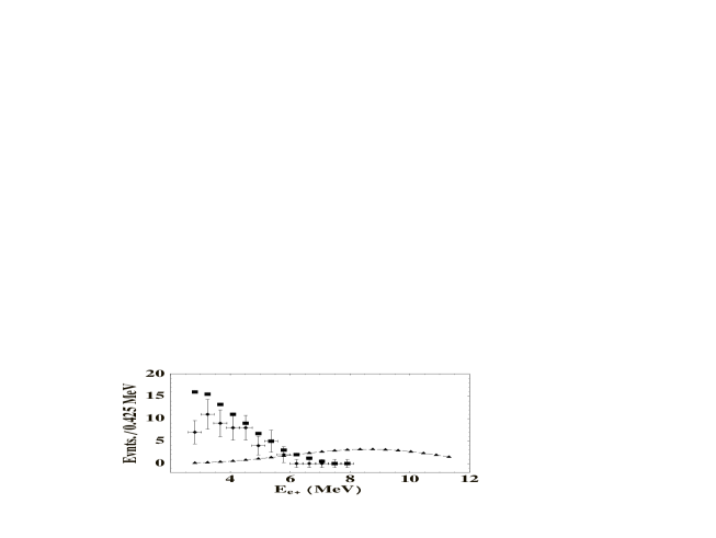
Figure 3: The solid squares represent the MC expectation of the KamLAND positron spectrum from reactor antineutrinos with no oscillations and the points with error bars represent the measured spectrum (from Fig.5 in Ref.[1]). Solid triangles represent the positron spectrum from solar antineutrinos (multiplied by 5) assuming profile 3 with peak field given by its 95% CL upper limit ($B_{0}=4.88\times 10^{7}G$). All curves refer to the same time exposure of 145 days.

Using the expected number of events in the first 145 days of data taking and in this energy range $(6-8.125)~{}MeV$, we have derived upper bounds on $B_{0}$ (90 and 95% CL) for all three profiles. They are shown in table 2 along with the upper bounds on $\mu_{\nu}B_{0}$ taking $\mu_{\nu}$ as a free parameter. The antineutrino flux upper bounds are now $\phi_{\bar{\nu}}<0.0049\phi(^{8}B)$ $\phi_{\bar{\nu}}<0.0055\phi(^{8}B)$ at 90 and 95% CL respectively. The KamLAND expected signal for an arbitrary field profile corresponding to 95% CL is shown in fig. 3.

The differences in magnitude among the bounds on $B_{0}$ and $\mu_{\nu}B_{0}$ presented in tables 1 and 2 for the different profiles are easy to understand. In fact, recalling that the ${}^{8}B$ production zone peaks at 5% of the solar radius and becomes negligible at approximately 15% (fig. 1), then in order to generate a sizeable antineutrino flux, the magnetic field intensity should lie relatively close to its maximum in the range where the neutrino production is peaked. Thus for profile 1 the value of $B_{0}$ required to produce the same signal is considerably larger than for the other two, while profile 3 is the most efficient one for antineutrino production.

As referred to above, for different field profiles the probability curves will differ only slightly in their shape if they lead to the same number of events. In other words, for a given number of events the probability curves are essentially the same, regardless of the field profile, a fact illustrated in fig. 2. As a consequence, the energy spectrum of the expected solar antineutrino flux will be nearly the same for any profile. In fig. 4 we plot this profile independent spectrum together with the ${}^{8}B$ one [13], so that a comparison can be made showing the shift in the peak and the distortion introduced.

4 Conclusions

To conclude, now that SFP is ruled out as a dominant effect for the solar neutrino deficit, it is important to investigate its still remaining possible signature in the solar neutrino signal, namely an observable $\bar{\nu}_{e}$ flux. Our main conclusion is that, from the antineutrino production model expound here, an upper bound on the solar antineutrino flux can be derived, namely $\phi_{\bar{\nu}}<3.8\times 10^{-3}\phi(^{8}B)$ and $\phi_{\bar{\nu}}<5.5\times 10^{-3}\phi(^{8}B)$ at 95% CL, assuming respectively Gaussian or Poissonian statistics. For 90% CL we found $\phi_{\bar{\nu}}<3.4\times 10^{-3}\phi(^{8}B)$ and $\phi_{\bar{\nu}}<4.9\times 10^{-3}\phi(^{8}B)$ which shows an improvement relative to previously existing bounds from LSD [19] by a factor of 3-5. These are independent of the detailed magnetic field profile in the core and radiative zone and the energy spectrum of this flux is also found to be profile independent. We also derive upper bounds on the peak field value which are uniquely determined for a fixed solar field profile. In the most efficient antineutrino producing case (profile 3), we get (95% CL) an upper limit on the product of the neutrino magnetic moment by the solar field $\mu_{\nu}B\leq 2.8\times 10^{-19}$ MeV or $B_{0}\leq 4.9\times 10^{7}G$ for $\mu_{\nu}=10^{-12}\mu_{B}$. A recent study of the magnetic field in the radiative zone of the sun has provided upper bounds of (3-7) MG [20] in that region in the vicinity of $0.2~{}R_{S}$ which are independent of any neutrino magnetic moment. Therefore we can use them in conjunction with our results to obtain a limit on $\mu_{\nu}$. Using $B_{0}\sim 3-7MG$, we get from the results for profiles 1-3: $\mu~{}\mbox{$\leq$}~{}0.7-9.6\times 10^{-12}\mu_{B}$. Moreover, from the limits obtained in this work, if the ’true’ solar profile resembles either a profile like 1 or 3, this criterion implies that SFP cannot be experimentally traced in the next few years, since the peak field value must be substantially reduced in order to comply with this upper bound, thus leading to a much too small antineutrino probability to provide an observable event rate . On the other hand, for a profile like 2 or in general any one resembling a dipole field, SFP could possibly be visible.

Acknowledgements. The work of BCC was supported by Fundação para a Ciência e a Tecnologia through the grant SFRH/BPD/5719/2001. E.T-L acknowledges many useful conversations with P. Aliani, M. Picariello and V. Antonelli, the hospitality of the CFIF (Lisboa) and the financial support of the Spanish CYCIT funding agency.

Profile	$S^{0}_{\bar{\nu}}(10^{7}G)$	$B_{0}(90\%CL)$	$B_{0}(95\%CL)$	$\mu_{\nu}B_{0}(90\%CL)$	$\mu_{\nu}B_{0}(95\%CL)$
		$G$	$G$	$MeV$	$MeV$
1.	$0.006$	$5.27\times 10^{8}$	$5.62\times 10^{8}$	$3.05\times 10^{-18}$	$3.25\times 10^{-18}$
2.	$0.137$	$1.14\times 10^{8}$	$1.21\times 10^{8}$	$6.60\times 10^{-19}$	$7.04\times 10^{-19}$
3.	$0.224$	$8.92\times 10^{7}$	$9.50\times 10^{7}$	$5.16\times 10^{-19}$	$5.50\times 10^{-19}$

Table 1: Solar antineutrino event rates, upper bounds on the peak field value for $\mu_{\nu}=10^{-12}\mu_{B}$ and on $\mu_{\nu}B_{0}$ for arbitrary $\mu_{\nu}$ and $B_{0}$, assuming Gaussian statistics in the whole KamLAND spectrum.

Profile	$S^{0}_{\bar{\nu}}(10^{7}G)$	$B_{0}(90\%CL)$	$B_{0}(95\%CL)$	$\mu_{\nu}B_{0}(90\%CL)$	$\mu_{\nu}B_{0}(95\%CL)$
		$G$	$G$	$MeV$	$MeV$
1.	$0.004$	$2.53\times 10^{8}$	$2.85\times 10^{8}$	$1.47\times 10^{-18}$	$1.65\times 10^{-18}$
2.	$0.079$	$5.56\times 10^{7}$	$6.25\times 10^{7}$	$3.22\times 10^{-19}$	$3.62\times 10^{-19}$
3.	$0.130$	$4.34\times 10^{7}$	$4.88\times 10^{7}$	$2.51\times 10^{-19}$	$2.82\times 10^{-19}$

Table 2: Same as table 1 assuming Poissonian statitics in the KamLAND energy range $E_{e}=(6-8.125)~{}MeV$.

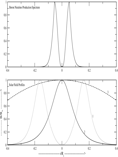
Figure 1: Upper panel: ${}^{8}B$ neutrino production spectrum (in arbitrary units) as a function of the radial coordinate. Lower panel: the three solar field profiles considered in the main text normalized to $B_{0}$, the peak field value.

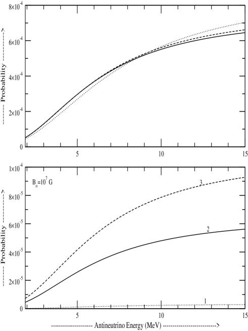
Figure 2: Antineutrino probabilities for solar field profiles 1, 2 and 3. Upper panel: the peak field is chosen in each case so as to produce the same event rate in KamLAND, (see the main text). Lower panel: the same value of the peak field ($B_{0}=10^{7}G$) is seen in each case to lead to probabilities of quite different magnitudes.

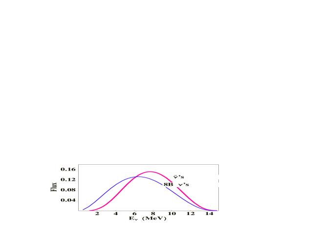
Figure 4: The expected solar antineutrino spectrum and the ${}^{8}B$ neutrino one [13], both normalized to unity, showing the peak shift and the distortion introduced by the antineutrino probability.

References

- [1] K. Eguchi et al. [KamLAND Collaboration], Phys. Rev. Lett. 90, 021802 (2003) [arXiv:hep-ex/0212021].
- [2] For reviews see e. g. Lino Miramonti and Franco Reseghetti, arXiv:hep-ex/0302035. E. K. Akhmedov, arXiv:hep-ph/9705451; J. Pulido, Phys. Rept. 211, 167 (1992). P. Aliani, V. Antonelli, R. Ferrari, M. Picariello and E. Torrente-Lujan, arXiv:hep-ph/0206308. S. Khalil and E. Torrente-Lujan, J. Egyptian Math. Soc. 9, 91 (2001) [arXiv:hep-ph/0012203]. E. Torrente-Lujan, arXiv:hep-ph/9902339.
- [3] P. Aliani, V. Antonelli, R. Ferrari, M. Picariello and E. Torrente-Lujan, Phys. Rev. D 67 (2003) 013006. P. Aliani, V. Antonelli, M. Picariello and E. Torrente-Lujan, Nucl. Phys. B634 (2002) 393-409. P. Aliani, V. Antonelli, M. Picariello and E. Torrente-Lujan, Nucl. Phys. Proc. Suppl. 110, 361 (2002). P. Aliani, V. Antonelli, R. Ferrari, M. Picariello and E. Torrente-Lujan, arXiv:hep-ph/0205061.
- [4] J. N. Bahcall, M. C. Gonzalez-Garcia and C. Pena-Garay, arXiv:hep-ph/0212147. P. Aliani, V. Antonelli, M. Picariello and E. Torrente-Lujan, arXiv:hep-ph/0212212. P. Aliani, V. Antonelli, M. Picariello and E. Torrente-Lujan, New J. Phys. 5 (2003) 2 [arXiv:hep-ph/0207348]. P. Aliani, V. Antonelli, R. Ferrari, M. Picariello and E. Torrente-Lujan, arXiv:hep-ph/0211062. A. Bandyopadhyay, S. Choubey, R. Gandhi, S. Goswami and D. P. Roy, arXiv:hep-ph/0212146. M. Maltoni, T. Schwetz and J. W. Valle, arXiv:hep-ph/0212129. G. L. Fogli, E. Lisi, A. Marrone, D. Montanino, A. Palazzo and A. M. Rotunno, arXiv:hep-ph/0212127. V. Barger and D. Marfatia, arXiv:hep-ph/0212126.
- [5] J. Schechter, J. W. F. Valle, Phys. Rev. D 24 (1981) 1883. J. Schechter, J. W. F. Valle, Phys. Rev. D 25 (1981) 283, Erratum.
- [6] C. S. Lim, W. J. Marciano, Phys. Rev. D 37 (1988) 1368.
- [7] E. Kh. Akhmedov, Sov. J. Nucl. Phys. 48 (1988) 382, Yad. Fiz. 48 (1988) 599 (in Russian). E. Kh. Akhmedov, Phys. Lett. B 213 (1988) 64.
- [8] B. C. Chauhan and J. Pulido, Phys. Rev. D 66, 053006 (2002) [arXiv:hep-ph/0206193]. E. Torrente-Lujan, arXiv:hep-ph/9912225. E. Torrente-Lujan, Phys. Rev. D 59, 093006 (1999). E. Torrente-Lujan, Phys. Rev. D 59, 073001 (1999). E. Torrente-Lujan, arXiv:hep-ph/9602398. V. B. Semikoz and E. Torrente-Lujan, Nucl. Phys. B 556, 353 (1999). E. Torrente-Lujan, arXiv:hep-ph/0210037. E. Torrente Lujan, Phys. Rev. D 53, 4030 (1996). B. C. Chauhan, arXiv:hep-ph/0204160. B. C. Chauhan, S. Dev and U. C. Pandey, Phys. Rev. D 59, 083002 (1999) [Erratum-ibid. D 60, 109901 (1999)]. E. K. Akhmedov and J. Pulido, Phys. Lett. B 529, 193 (2002). J. Pulido, Astropart. Phys. 18, 173 (2002). E. K. Akhmedov and J. Pulido, Phys. Lett. B 485, 178 (2000).
- [9] E. Kh. Akhmedov, Sov. J. JETP 68 (1989) 690, Zh. Eksp. Teor. Fiz. 95 (1989) 1195 (in Russian). R. S. Raghavan, et al., Phys. Rev. D 44 (1991) 3786. C. S. Lim et al., Phys. Lett B 243 (1990) 389. E. Kh. Akhmedov, S. T. Petcov, A. Yu. Smirnov, Phys. Rev. D 48 (1993) 2167, hep-ph/9301211.
- [10] E. Torrente-Lujan, arXiv:hep-ph/0302082. E. Torrente-Lujan, Phys. Lett. B 441, 305 (1998). P. Aliani, V. Antonelli, M. Picariello and E. Torrente-Lujan, JHEP 0302:025,2003. E. Torrente-Lujan, Nucl. Phys. Proc. Suppl. 87, 504 (2000). E. Torrente-Lujan, Phys. Lett. B 494, 255 (2000) [arXiv:hep-ph/9911458].
- [11] E. K. Akhmedov and J. Pulido, Phys. Lett. B 553, 7 (2003) [arXiv:hep-ph/0209192].
- [12] See, e.g., G. G. Raffelt, Phys. Rev. Lett. 64, 2856 (1990); G. G. Raffelt, Phys. Rept. 320, 319 (1999). V. Castellani and S. Degl’Innocenti, Astrophys. J. 402, 574 (1993).
- [13] J.N.Bahcall’s homepage, http://www.sns.ias.edu/jnb/.
- [14] G.Horton-Smith, Neutrinos and Implications for Physics Beyond the Standard Model, Stony Brook, Oct. 11-13, 2002. http://insti.physics.sunysb.edu/itp/conf/neutrino.html A.Suzuki. Texas in Tuscany, XXI Symposium on Relativistic Astrophysics Florence, Italy, December 9-13, 2002. http://www.arcetri.astro.it/ texaflor/.
- [15] P. Vogel and J. F. Beacom, Phys. Rev. D 60, 053003 (1999) [arXiv:hep-ph/9903554].
- [16] J. Pulido and E. K. Akhmedov, Astropart. Phys. 13, 227 (2000) [arXiv:hep-ph/9907399].
- [17] G. J. Feldman and R. D. Cousins, Phys. Rev. D 57, 3873 (1998) [arXiv:physics/9711021].
- [18] K. Hagiwara et al. [Particle Data Group Collaboration], Phys. Rev. D 66, 010001 (2002).
- [19] M. Aglietta et al., JETP Lett. 63 (1996) 791, Pisma Zh. Eksp. Teor. Fiz. 63 (1996) 753 (in Russian).
- [20] A. Friedland and A. Gruzinov, arXiv:astro-ph/0211377.