Baryogenesis at the electroweak phase transition

Abstract

A possible solution to the observed baryon asymmetry in the universe is described, based on the physics of the standard model of electroweak interactions. At temperatures high enough electroweak physics provides violation of baryon number, while $C$ and $CP$ symmetries are not exactly conserved, although in the context of the minimal electroweak model with one Higgs doublet the rate of $CP$ violation is not sufficient enough to generate the observed asymmetry. The condition that the universe must be out of thermal equilibrium requires the electroweak phase transition (EWPT) to be first order. The dynamics of the phase transition in the minimal model is investigated through the effective potential, which is calculated at the one loop order. Finite temperature effects on the effective potential are treated numerically and within the high temperature approximation, which is found to be in good agreement with the exact calculation. At the one loop level the phase transition was found to be of the first order, while the strength of the transition depends on the unknown parameters of the theory which are the Higgs boson and top quark masses top  .

“Why does the whole world have $<\phi>=+v$? Why doesn’t it have $<\phi>=-v$ somewhere? Suppose that God created the universe in the state $<\phi>=0$ and then the universe discovered that it could lower its energy; Where it puts its energy is none of my business, but it gets rid of it – gives it back to God or something;”

R. Feynman Feynman:1976

I The Baryogenesis Problem

I.1 Overview

Recently the connection between particle physics and cosmology has received much attention. The classical cosmological model of the expanding universe provides a powerful framework where particle physics can test its predictions about matter genesis. The expansion of the universe can be considered as an enormous particle accelerator, which although ran billions of years ago in the far past, can still be used to check the validity of theories concerning the elementary particles. Cosmology on the other hand can use the predictions of particle physics about the nature and behaviour of the elementary particles in order to cure unsolved up to now cosmological problems which are involved in the theories concerned with the evolution of the universe.

The baryogenesis problem, that is the observed excess of matter over antimatter today in the universe, is one of these problems. As pointed out by Sakharov in 1967 Sakharov:dj , the universe began in a baryon symmetric state but particle interactions produced a net asymmetry. He postulated three conditions to be satisfied in order to explain the observed baryon excess. These are: (a) baryon number non–conservation, (b) $C$ and $CP$ violation and (c) that the universe must be out of thermal equilibrium. Our aim is to explore how these conditions are satisfied in the framework of the standard model of electroweak interactions. We will focus our attention on the third condition and provide a careful study of the electroweak phase transition. Our main goal is to examine the order of this transition when temperature is introduced in the model via the so–called one loop approximation.

This work is organized as follows: In order to establish the basic principles for the baryogenesis problem the remainder of this section is devoted to a brief account on the development of the big bang model, the standard cosmological model, from its beginning up to the present days. The most important stages in the development of the big bang model are given in Section I.2. In Section I.3 we present how the baryogenesis problem appears in the framework of the standard big bang cosmology. The necessity to satisfy the Sakharov conditions and relevant comments are outlined in Section I.4. A recent development in the standard hot big bang model, the inflation model, is discussed briefly in Section I.5.

According to recent investigations it is possible that the necessary conditions for the solution of the baryogenesis problem can be satisfied in the standard model of the electroweak interactions, so we find very useful to provide an introduction to the standard model of these interactions and its connection with cosmology. This is the subject of Section II, where phase transitions in gauge theories are also discussed briefly through well known examples.

The standard electroweak model satisfies the first two conditions, so we sketch in Section III how baryon number and $CP$ symmetry are violated in the model. In the standard model, due to the non–trivial structure of the $SU(2)$ gauge vacuum and as a consequence of anomalous processes, baryon number is not conserved. On the other hand $CP$ symmetry is violated in the standard model because of relative phases between the electroweak gauge interactions and the Higgs interactions of the quarks.

The third condition is satisfied if the electroweak phase transition (EWPT) is of the first order. The basic tool for the investigation of the electroweak phase transition is the finite temperature effective potential, the quantity which has the meaning of the free energy density of the system under consideration, and the relevant theory is given in some detail in Section IV.

The evolution and the order of the electroweak phase transition will be determined in the so–called one loop approximation in Section V. Finite temperature effects are treated exactly and within the high temperature limiting case.

The last section is devoted to a discussion concerning our investigation of the electroweak phase transition in connection with the baryogenesis problem and we also present there a summary of our results and conclusions.

I.2 The Hot Big Bang

Modern cosmological theories started to develop within the framework of Einstein’s general theory of relativity early this century. The development of particle physics in the recent years has infused new ideas in cosmology, which can be applied to the study of the earliest moments of the universe and the evolution to its present state. The most accepted up to date cosmological theory is the hot big bang model. This theory is based upon general relativity and the Friedmann model for an expanding universe. According to this model the universe starts its life from a state of enormous matter density and temperature and after its expansion results in what we observe today. The evolution and the most important stages in the development of this cosmological theory up to the present days have been explored in an elegant way by many authors Hawking:1988 ; Weinberg:1976 ; Parker:1988 .

A detailed discussion on the formulation of this theory is given by Weinberg Weinberg:1972 and Kolb and Turner Kolb:1990 , while a brief account can be found in Linde Linde:1990 . The beginning of the theory and the first important stage goes back in 1922 when Friedmann based on Einstein’s cosmological principle, which is the hypothesis that the universe is spatially homogeneous and isotropic, and created a model for an expanding universe. A few years later, Hubble’s and Slipher’s observations of the galactic redshift supported experimentally the idea of the expansion from an initial state and very soon this theory became the cornerstone of modern cosmology.

In Friedmann’s model the radius of the universe $R=R(t)$, or more explicitly its scale factor, is a function of time and has an evolution which is described by the equations of general relativity. Einstein’s equations imply an evolution for the scale factor given by the first order differential equation

$$\dot{R}+k=\frac{8\pi G}{3}\rho R^{2}~{}.$$ (1)

The constant $k$ in the above equation describes the curvature of space and takes the values $k=-1,\;0,\;1$, which correspond to open, flat and close universe models respectively and $G$ is the gravitational constant. In addition we have an energy conservation law which can be expressed by

$$\dot{\rho}R^{3}+3(\rho+p)R^{2}\dot{R}=0~{},$$ (2)

where $\rho$ is the energy density of matter in the universe and $p$ its pressure. In order to solve these equations and find out how the universe evolves in time, we need a state equation which relates the energy density of the universe to its pressure. We may assume $p=\omega\rho$ so the above equations give the result

$$\rho\sim R^{-3(1+\omega)}~{}.$$ (3)

We can consider two possibilities, in order to interpret this solution. If we suppose that the universe was filled with nonrelativistic cold matter with negligible pressure $p=0$, we find that $\rho\sim R^{-3}$. If the universe was a hot ultrarelativistic gas of noninteracting particles with $p=\rho/3$, we then find that $\rho\sim R^{-4}$. When $R$ is small one finds that for nonrelativistic cold matter the radius of the universe evolves in time as $R\sim t^{2/3}$, while in the case of the hot ultrarelativistic gas it goes as $R\sim t^{1/2}$. Thus regardless the model used, as the time $t$ tends to zero, the scale factor vanishes and the density of matter becomes infinite. The point $t=0$ is known as the initial cosmological singularity. It is the initial point when the universe starts its life and then expands to what it is today. The expansion rate of the universe is given by the quantity $H=\dot{R}/R$ which is known as the Hubble constant, although it is not really a constant but it varies with time.

Up to the mid–sixties it was not clear if the universe had started its life from a hot or a cold initial state. The new era in cosmology opened when Penzias and Wilson discovered the $2.7^{0}K$ microwave background radiation in 1964–65, which had been predicted by the hot universe theory. If we suppose that the universe expanded adiabatically, then during the expansion the quantity $RT$ remained approximately constant, and the temperature of the universe dropped off as $T\sim R^{-1}(t)$. The radiation which was detected by Penzias and Wilson were the relic photons of the initially hot photon gas which cooled down during the expansion of the universe. This was the second stage in the development of modern cosmology and was decisive in the establishment of the hot big bang model as the standard cosmological model.

I.3 Baryon Asymmetry in the Universe

Although the standard hot big bang model is successful in accounting for Hubble expansion, the residual microwave background radiation and the abundances of light atomic nuclei there remain some serious difficulties and one of these open questions is the observed baryon asymmetry in the universe today. The essence of the baryon asymmetry problem is to understand why in the observable part of the universe the density of baryons is many orders greater than the density of antibaryons and why on the other hand the density of baryons is much less than the density of photons Kolb:1990 . The baryon asymmetry can be quantified by a quantity known as the baryon number $B$ of the universe and is defined as the ratio of the baryon number density $n_{B}$ to the entropy density $s$. The baryon number density $n_{B}$ is defined as the number density of baryons $n_{b}$ minus the number density of antibaryons $n_{\overline{b}}$, so $n_{B}=n_{b}-n_{\overline{b}}$. The baryon number of the universe today, is estimated in the range Kolb:1990 ; Kolb:ni [See however in Section VI.3]

$$B=\frac{n_{B}}{s}\sim(6-10)\times 10^{-11}~{}.$$ (4)

There is a strong evidence of the asymmetry since it is well known that the earth as well as all the objects on it consist of matter rather than antimatter. It is an experimental fact that there is no antimatter on the earth and the outer space. Measurements of the cosmic rays emitted from the sun have proven the absence of antimatter in the solar system. Only an insignificant positron flux is contained in solar cosmic rays and it is mainly due to interactions of the primary solar cosmic rays with matter.

Astronomical observations show that at least our galaxy consists of usual matter, while an inconsiderable amount of antimatter is observed and does not seem to indicate the presence of antimatter in the galaxy. For clusters of galaxies and their intergalactic gas one can derive limits for the amount of antimatter present from the $\gamma$ flow expected from the $\pi{{}^{0}}$ decay, since matter–antimatter annihilation would produce $\pi^{0}$ mesons and those decay into $\gamma$–rays. These hard photons have never been observed. It is not definite if there are in our universe islands of antimatter separated by empty space of regions containing normal matter. Electromagnetic radiation which is the main source of informations from the outer space cannot give a signal about its matter or antimatter origin.

I.4 Three Cornerstones of Baryogenesis

In Friedman’s cosmology the excess of matter over antimatter is considered as one of the initial conditions and the baryonic asymmetry as one of the fundamental cosmological constants. This philosophy changed in early seventies when Sakharov and others suggested that the observed asymmetry could be generated dynamically even though the universe had started in an initially symmetric state. Sakharov postulated three necessary conditions for this to happen:

(a) There must be baryon number violating processes.
(b) Breaking of charge $(C)$ and combined $(CP)$ symmetries.
(c) These processes must go out of equilibrium sometime during the history of the universe.

The first condition is obvious since it is clear that the baryon number must be violated if the universe started its life in a baryon symmetric state and then evolved into an asymmetric one. Many models predict baryonic asymmetry Dolgov:1991fr , although baryon number violation has never been verified experimentally. In Grand Unified Theories (GUT) baryon number violation occurs in the equations of motion of the theory. It proceeds with the exchange of very massive particles and takes place at an energy scale of the order of magnitude about ${10}^{16}\,\textrm{GeV}$. Supersymmetric models also predict baryon non conserving processes in the energy range $10^{16}\,\textrm{GeV}$– $10^{2}\,\textrm{GeV}$ depending upon the concrete model.

In order to understand the necessity of the second condition we note that the baryon number of a state is odd under $C$ and combined $CP$ symmetries. That is, the baryon number of a state changes sign under charge conjugation $C$ and charge conjugation combined with parity $CP$. Thus if a state is either $C$ or $CP$ invariant, then the baryon number of this state should be zero. If the universe begins its life with equal amounts of matter and antimatter, and without a preferred direction, then its initial state is both $C$ and $CP$ invariant. Unless both $C$ and $CP$ are violated, the universe will remain $C$ and $CP$ invariant as it evolves to its final state, and thus cannot develop a net baryon number even if the baryon number is not conserved. Therefore both $C$ and $CP$ violations are needed if a net excess of matter over antimatter is to be produced. In contrast to baryon number violation, which has only been predicted in various theoretical models but with no experimental evidence for it, $C$ and $CP$ violation have been verified experimentally in neutral Kaon decays.

The necessity to satisfy the last Sakharov condition, that the universe must be out of thermal equilibrium, is very important, since if an initially baryonic symmetric universe is in thermal equilibrium, then particle number densities are given by

$$n_{eq}=\frac{1}{\exp[(E-\mu)/T]\pm 1}~{},$$ (5)

where $E$ is the particle energy and $\mu$ its chemical potential. If the charge is not conserved the corresponding chemical potential vanishes in equilibrium. $CPT$ invariance guarantees that particles and antiparticles have the same mass, therefore their number remains equal during the expansion and so no asymmetry occurs, regardless of $B$, $C$, or $CP$ violating processes.

I.5 The Inflation Model

The development of gauge theories and their influence to the cosmological questions led to the development of a new version of the standard big bang model. The inflation model which was introduced by Guth in 1981 Guth:1980zm came to cure some of the pathological problems of the hot universe theory. According to this model, soon after the beginning of the big bang the expansion rate of the universe increases exponentially, and due to this expansion the universe supercools and all the physical processes are interrupted. Then the universe reheats again and continues its expansion with a slower rate.

A detailed analysis of the inflation model is given by Linde Linde:1990 ; Linde:ir , while important papers relevant to this model (and not only) are collected by Abbott and Pi Abbott:kb . Although the inflation model is not the subject of this work, we should note here that it has already solved many of the problems that the hot big bang model possesses. On the other hand the inflation model imposes the constraint that the baryon generation should have occurred after the exponential expansion, since the creation of a large amount of entropy during the inflation epoch would dilute any pre–existing baryon asymmetry. If one believes the inflation model then baryogenesis should happen at rather lower scale energies than those of the GUT’s scale. This is especially gratifying for present day investigations, since our technology makes only electroweak energy scales, not GUT’s scales, accessible to experimental tests.

II Gauge Theories and Cosmology

II.1 Introduction

The experimental success of the model of unified electroweak interactions and the development of unified gauge theories of all the interactions at the beginning of the seventies opened a new era for the theories of the elementary particles. The creation and evolution of these theories have their roots on symmetry principles. Generalization of the ideas about symmetries generated the gauge principle and the present belief that all particle interactions are dictated by the so–called local gauge symmetries. This principle arises from the requirement that all quantities which are conserved, are conserved locally and not merely globally.

Gauge invariant Lagrangians describing particle interactions remain invariant under a set of local gauge transformations. But invariance of the Lagrangian demands for the particles to be massless. The particles become massive due to the appearance of constant classical scalar fields $\phi$ over all space, through the so–called mechanism of symmetry breaking.

The rapid development of particle physics not only led to a better understanding of particle interactions, but also to a significant progress in the theories of superdense matter, matter more than 80 orders of magnitude denser than the nuclear matter. It was Kirzhnits and Linde Kirzhnits:ut and very soon others Dolan:qd ; Weinberg:hy who showed that the scalar fields which are responsible for the breaking of symmetry, could disappear at high enough temperatures. This means that at temperatures high enough phase transitions take place and after they have been completed, the symmetry is restored.

These theories are applicable in cosmology since superdense matter at very high energies and temperatures should appear at very early stages of the evolution of the universe. According to the standard hot big bang model for an expanding universe, as the universe cools down these phase transitions could take place. Cosmological problems, as the baryon excess for example, could find an answer in the framework of gauge theories. Recent development in this area suggest that the baryogenesis problem could find its answer in the standard model of electroweak interactions. This model possesses baryon number violation as it was proved by t’Hooft 'tHooft:up ; 'tHooft:fv , although the violation rate at zero temperatures seems to be too small. Violation of the $CP$ symmetry is provided by the Cabbibo–Kobayashi–Maskawa mixing between the quark families. The condition that the system must be out of equilibrium demands the electroweak phase transition to be of the first order.

The remainder of this section is devoted on the formulation of the electroweak theory and an introduction to the theory of phase transitions in gauge theories. In the next section we discuss the formulation of the standard electroweak model as a gauge theory. The mechanism of symmetry breaking and the generation of particle masses are presented in Sections II.3 and II.4 respectively. The idea of symmetry restoration at high temperatures and a brief discussion of the cosmological phase transitions are contained in the last two Sections II.5 and II.6 .

II.2 Electroweak Gauge Theory

The successful formulation of Quantum Electrodynamics (QED) as a gauge theory led to the idea of extending the gauge principle to the description of other interactions. Constructing a gauge theory we demand the Lagrangian to be locally invariant under a group of internal symmetries. Thus we introduce into the Lagrangian a number of vector fields equal to the number of the symmetry group generators. The gauge bosons self–interactions as well as the way they couple to matter fields is completely determined by the gauge couplings. The QED Lagrangian for example is invariant under a set of local $U(1)$ transformations with generator $Q$, the electric charge operator. Invariant interactions are mediated by one vector field, the photon field. In Quantum Chromodynamics (QCD), the gauge theory of strong interactions, we introduce eight vector fields (the gluon fields) into the Lagrangian and the theory is based on the group $SU(3)$, which has eight generators the Gell–Mann matrices.

The Glashow–Salam–Weinberg model which unifies the weak and electromagnetic interactions, known as the standard model of electroweak interactions, is based on the non–Abelian group $SU(2)_{L}\times U(1)_{Y}$ and has four generators. The weak interactions are mediated by three vector bosons $A^{a}_{\mu},\;a=1,2,3$ which are accommodated in the adjoint representation of an $SU(2)$ group denoted by $SU(2)_{L}$ with generators $T_{a}=\tau_{a}/{2}$, where the $\tau_{a}$, $a=1,2,3$ are the Pauli matrices and the $T_{a}$ are referred as the weak isospin generators. The subscript $L$ signifies that the $A_{\mu}^{a}$ couple in a parity violating way to the left handed parts of the lepton matter fields, which transform as a doublet again under the same $SU(2)_{L}$.

To accomodate the electromagnetic interactions we need another gauge boson $B_{\mu}$ and another group denoted by $U(1)_{Y}$. The generator of the $U(1)_{Y}$ group is $Y/2$, where $Y$ is the weak hypercharge defined through the so–called Gell–Mann–Nishijima relation as

$$Q=T_{3}+Y/2$$ (6)

and $T_{3}$ is the third component of the weak isospin. The gauge coupling for the weak isospin group $SU(2)_{L}$ is denoted by $g$ and that for weak hypercharge group $U(1)_{Y}$ as $g^{\prime}/2$. The kinetic terms into the Lagrangian for the two gauge fields are

$$\mathcal{L}_{gauge}=-\frac{1}{4}F^{a}_{\mu\nu}F^{a\mu\nu}-\frac{1}{4}B_{\mu\nu}B^{\mu\nu}~{},$$ (7)

where the field strength tensor for the $SU(2)_{L}$ gauge field is given by

$$F^{a}_{\mu\nu}=\partial_{\mu}A^{a}_{\nu}-\partial_{\nu}A^{a}_{\mu}+g\epsilon^{abc}A^{b}_{\mu}A_{\nu}^{c}~{},$$ (8)

while the field strength tensor of the $U(1)_{Y}$ gauge field has the form

$$B_{\mu\nu}=\partial_{\mu}B_{\nu}-\partial_{\nu}B_{\mu}~{}.$$ (9)

The physical particles which mediate the weak and electromagnetic interactions, the two charged $W^{+}$ and $W^{-}$, the neutral $Z^{0}$ and the photon $\gamma$ result as linear combinations of the fields $A^{a}_{\mu}$ and $B_{\mu}$.

The fermionic matter fields are present in the model grouped in three families or generations which include the $e,\;\nu_{e},\;u,\;d$ known as first generation and other two replications the $\mu,\;\nu_{\mu},\;c,\;s$ family and the $\tau,\;\nu_{\tau},\;t,\;b$ family. Violation of the parity is introduced into the model by putting the left–handed and right–handed fermions into different group representations. All the left–handed fields are taken to transform as doublets under $SU(2)_{L}$, while the right–handed fermions transform as singlets.

The left–handed quarks are introduced into the model grouped into $SU(2)$ doublets of the form

$$Q_{u}=\left(\begin{array}[]{l}u\\ d^{\prime}\end{array}\right)\qquad Q_{c}=\left(\begin{array}[]{c}c\\ s^{\prime}\end{array}\right)\qquad Q_{t}=\left(\begin{array}[]{r}t\\ b^{\prime}\end{array}\right)~{}.$$ (10)

The prime means that these are weak eigenstates, which are constructed as linear combinations of the mass eigenstates. The matrix which connects the two sets of eigenstates is referred as the Cabbibo–Kobayashi–Maskawa (CKM) matrix. By convention the charge 2/3 quarks are unmixed, but the eigenstates of the charge $-1/3$ quarks are related through the CKM matrix as

$$\left(\begin{array}[]{c}d^{{}^{\prime}}\\ s^{{}^{\prime}}\\ b^{{}^{\prime}}\end{array}\right)=K\left(\begin{array}[]{c}d\\ s\\ b\end{array}\right)~{}.$$ (11)

This mixing is very significant for violation of the $CP$ symmetry in the the standard electroweak model which we discuss in the next chapter. The right–handed quarks are $SU(2)$ singlets with hypercharge $Y=4/3$ for the charge $Q=2/3$ quarks $u_{R},c_{R}$ and $t_{R}$ since the charge $Q=-1/3$ quarks $d^{\prime}_{R},s^{\prime}_{R}$ and $b^{\prime}_{R}$ have hypercharge $Y=-2/3$.

In a similar way the left-handed leptons are present in the model grouped in $SU(2)$ doublets of the form

$$L_{e}=\left(\begin{array}[]{l}\nu_{e}\\ e\end{array}\right)\qquad L_{\mu}=\left(\begin{array}[]{c}\nu_{\mu}\\ \mu\end{array}\right)\qquad L_{\tau}=\left(\begin{array}[]{r}\nu_{\tau}\\ \tau\end{array}\right)$$ (12)

where the left–handed lepton states are $l_{L}=\frac{1}{2}(1-\gamma^{5})l$ and $l$ stands for $e,\;\mu,\;\tau$ and the corresponding neutrinos. The right–handed leptons are weak isospin singlets of the form $l_{R}=\frac{1}{2}(1+\gamma^{5})l$. The $l$ now stands for the $e,\;\mu,\;\tau$, since it is convenient to idealize the neutrinos as massless and in this case right–handed neutrinos do not exist. In order to satisfy the Gell–Mann–Nishijima relation for the lepton charge the left–handed leptons have hypercharge $Y_{L}=-1$, whilst to the right–handed we assign hypercharge $Y_{R}=-2$ .

As a conclusion to the above discussion, the fermion part of the Lagrangian can be written as

$$\mathcal{L}_{f}= \sum_{f_{L}}\overline{f}_{L}\gamma^{\mu}\left(i\partial_{\mu}-g\frac{\tau_{a}}{2}A^{a}_{\mu}-g^{\prime}\frac{Y}{2}B_{\mu}\right)f_{L}$$ (13)

$$+\sum_{f_{R}}\overline{f}_{R}\gamma^{\mu}\left(i\partial_{\mu}-g^{\prime}\frac{Y}{2}B_{\mu}\right)f_{R}~{},$$

where the sum runs over all left– and right–handed fermion fields. Addition of the gauge and fermion parts results in a Lagrangian density which describes massless gauge boson fields interacting with massless fermionic matter fields.

Gauge boson mass terms which should be of the form $\frac{1}{2}M_{B}^{2}B_{\mu}B^{\mu}$ plus similar terms for the $A^{i}_{\mu}$ are clearly not gauge invariant. In addition a fermion mass term should be of the form

$$-m\overline{f}f=-m(\overline{f}_{R}f_{L}+\overline{f}_{L}f_{R})~{}.$$ (14)

Such a term manifestly breaks the gauge chiral invariance, since $f_{L}$ is a member of a $SU(2)_{L}$ doublet whilst $f_{R}$ is a singlet. Thus addition of mass terms by hand into the Lagrangian destroys the gauge invariance and the resulting theory is not renormalisable. However, it is an experimental fact that the vector bosons which mediate the weak interactions and the fermions are massive particles. The answer to the crucial problem of the mass generation without loosing the renormalisability of the theory is the Higgs mechanism, which is discussed in the next section.

II.3 Spontaneous Symmetry Breaking

The only known renormalisable theories involving vector bosons are gauge theories, but since mass terms in the Lagrangian spoil the gauge invariance it is impossible to find a renormalisable theory of massive vector bosons. However, it is possible for the Lagrangian and the equations of motion of a system to have a symmetry but the solutions of the equations to violate this symmetry. This phenomenon, where the solutions violate the symmetry of the equations, is known as spontaneous symmetry breaking (SSB). A well known example is the case of a ferromagnet, where the Hamiltonian of the system is rotationally invariant, but the ground state of the system has a non zero magnetization and it is clearly not invariant under rotations. The analogous of the ground state of the ferromagnet in particles physics is of course the vacuum. The Lagrangian of the theory is taken to be invariant under an internal symmetry, but the vacuum state is not. The ground state is characterised by some scalar fields which are not invariant under the symmetry transformations and develop a non zero vacuum expectation value.

Consider the case of one scalar field with quartic self interaction. The Lagrangian of the theory is given by

$$\mathcal{L}=\frac{1}{2}(\partial_{\mu}\phi)^{2}-\frac{1}{2}m^{2}\phi^{2}-\frac{1}{4}\lambda\phi^{4}~{},$$ (15)

where $m$ is the field mass and $\lambda$ its coupling constant. The potential energy density of this field at the classical level, which is called the classical potential is given by

$$V_{0}=\frac{1}{2}m^{2}\phi^{2}+\frac{1}{4}\lambda\phi^{4}~{}.$$ (16)

The Lagrangian remains invariant under the the symmetry operation which replaces $\phi$ by $-\phi$.

Let us consider now two cases and first suppose that the mass squared of the field is positive, $m^{2}=\mu^{2}>0$. From Eq. (16) it is clear that the potential has a minimum, which is the most favourable state of the system, for $\phi=0$. The minimum of the potential is shown in Fig. 1 .

Figure 1: The classical potential $V_{0}(\phi)$ before symmetry breaking.

But in the case when the mass squared is negative, that is $m^{2}=-\mu^{2}<0$, we observe a very different situation . The potential energy has two minima which occur at $\phi=\sigma=\pm\mu/\sqrt{\lambda}$ and now there are two degenerate ground states. Once we choose one of them, the ground state does not share the symmetry with the Lagrangian.This situation is illustrated in Fig. 2.

Figure 2: The classical potential $V_{0}(\phi)$ after symmetry breaking.

The value of the curvature of the potential near the extrema describes the effective mass squared of the scalar fluctuations. Prior the symmetry breaking the mass term of the field is negative. After breaking of symmetry the mass term becomes positive

$$m^{2}(\phi=\sigma)=\frac{d^{2}V}{d\phi^{2}}\bigg{|}_{\phi=\sigma}=3\lambda\sigma^{2}-\mu^{2}=2\mu^{2}>0~{}.$$ (17)

In determining masses and interactions one must perturb about the stable vacuum by shifting the field $\phi$ as $\phi(x)=\sigma+\eta(x)$ . Inserting that into the Lagrangian, the mass term appears with the correct sign. The above example serves as a useful introduction to symmetry restoration at high temperatures, which we discuss in Section II.5.

II.4 Boson and Fermion Masses

In order to understand the problem of mass generation for fermions and vector bosons we review here the well known Higgs model. In the simple scalar model, which we examined earlier, the mass term after symmetry breaking appeared with the correct sign. In the Higgs model insertion of the scalar field into the Lagrangian results in the generation of masses for the particles which interact with. The Lagrangian of this model exhibits a $U(1)$ gauge symmetry and is given by

$$\mathcal{L} = (\partial^{\mu}+igA^{\mu})\phi^{*}(\partial_{\mu}-igA_{\mu})\phi-\frac{1}{4}F_{\mu\nu}F^{\mu\nu}$$ (18)

$$-\mu^{2}\phi^{*}\phi-\lambda(\phi^{*}\phi)^{2}~{}.$$

For $\mu^{2}>0$ the Lagrangian, apart from the scalar self interaction term, is that of scalar QED. However, in the case where $\mu^{2}<0$, shifting the field to its true ground state as

$$\phi(x)=\frac{1}{\sqrt{2}}[\sigma+\eta(x)+i\xi(x)]$$ (19)

and inserting that into the Lagrangian, the latter becomes

$$\mathcal{L}^{\prime} = \frac{1}{2}(\partial_{\mu}\xi)^{2}+\frac{1}{2}(\partial_{\mu}\eta)^{2}-\frac{1}{4}F_{\mu\nu}F^{\mu\nu}$$ (20)

$$-\lambda\sigma^{2}\eta^{2}+\frac{1}{2}g^{2}\sigma^{2}(A_{\mu})^{2}-g\sigma A_{\mu}\partial_{\mu}\xi$$

where for simplicity we have omitted the interaction terms. The particle spectrum in the new Lagrangian appears to be composed by a massless scalar, the so-called Goldstone boson, a massive scalar particle $\eta$ with mass $m_{\eta}=\sqrt{2\lambda\sigma^{2}}$ and a massive vector $A^{\mu}$ with mass $m_{A}=g\sigma$.

One can use the freedom of a gauge transformation to eliminate the unphysical Goldstone mode. Then the Lagrangian looks like

$$\mathcal{L}^{\prime\prime} = \frac{1}{2}(\partial_{\mu}h)^{2}-\lambda\sigma^{2}h^{2}+\frac{1}{2}g^{2}\sigma^{2}A_{\mu}^{2}-\lambda\sigma h^{3}-\frac{1}{4}\lambda h^{4}$$ (21)

$$+\mbox{}\frac{1}{2}g^{2}A_{\mu}^{2}h^{2}+\sigma g^{2}A_{\mu}^{2}h-\frac{1}{4}F_{\mu\nu}F^{\mu\nu}.$$

The Goldstone boson no longer appears in the theory and the Lagrangian describes just two interacting massive particles. The particle spectrum consists of a massive vector boson $A_{\mu}$ and a massive scalar $h$, which is known as a Higgs particle.

The mechanism we have presented above, is known as the Higgs mechanism. An overview of the model can be found for example in Halzen and Martin Halzen:mc or Cheng and Li Cheng:bj . The Higgs mechanism can be generalized to non Abelian gauge theories and in particular to the case of the standard model of electroweak interactions. We present how, due to spontaneous breaking of symmetry, the fermions and vector bosons acquire their masses. In the case of the so–called minimal standard model, one complex $SU(2)$ doublet of scalar fields, with hypercharge $Y=1$ is introduced,

$$\Phi=\left(\begin{array}[]{c}\phi^{+}\\ \phi^{0}\end{array}\right)=\frac{1}{\sqrt{2}}\left(\begin{array}[]{c}\phi_{1}+i\phi_{2}\\ \phi_{3}+i\phi_{4}\end{array}\right)~{},$$ (22)

where $\phi,\;\;i=1,2,3,4$ are real fields. The building block of the Lagrangian containing the scalar doublet looks like

$$\mathcal{L}_{\phi}=(D^{\mu}\Phi)^{{\dagger}}(D_{\mu}\Phi)-V(\Phi)~{},$$ (23)

where the covariant derivative is given by

$$D_{\mu}=\partial_{\mu}-i\frac{g}{2}\tau^{a}A^{a}_{\mu}-i\frac{g^{\prime}}{2}B_{\mu}$$ (24)

and the most general gauge–invariant renormalisable potential is of the form

$$V(\Phi)=-\mu^{2}\Phi^{{\dagger}}\Phi+\lambda(\Phi^{{\dagger}}\Phi)^{2}~{},$$ (25)

with the mass $\mu^{2}$ being positive. Without loss of generality the minimum of the field $\Phi$ can be chosen at

$$\Phi=\frac{1}{\sqrt{2}}\left(\begin{array}[]{c}0\\ \sigma\end{array}\right)~{},$$ (26)

where $\sigma^{2}=\mu^{2}/\lambda$ and since we are interested in the physical particle spectrum the unitary gauge is an appropriate choice. Just as in the case of the Higgs model, after spontaneous breaking of symmetry the kinetic term of the scalar part of the Lagrangian $(D^{\mu}\Phi)^{{\dagger}}(D_{\mu}\Phi)$ gives rise to the vector boson masses. The two charged vector bosons are defined by the combination

$$W^{\pm}_{\mu}=\frac{1}{\sqrt{2}}(A^{1}_{\mu}\pm iA^{2}_{\mu})$$ (27)

with a classical mass

$$m_{W}=\frac{1}{2}g\sigma~{},$$ (28)

where $\sigma$ is the vacuum expectation value of the Higgs field. The neutral vector boson field appears as the combination

$$Z_{\mu}=\frac{g^{\prime}B_{\mu}-gA^{3}_{\mu}}{\sqrt{g^{2}+g^{\prime^{2}}}}$$ (29)

and its classical mass is given by

$$m_{Z}=\frac{1}{2}(g^{2}+g^{\prime^{2}})^{1/2}\sigma.$$ (30)

The photon field remain massless $m_{A}=0$ and is given by the combination

$$A_{\mu}=\frac{g^{\prime}B_{\mu}+gA^{3}_{\mu}}{\sqrt{g^{2}+g^{\prime^{2}}}}~{}.$$ (31)

The generation of the fermion masses can be done in a similar way. For this we introduce into the Lagrangian Yukawa coupling terms between scalars and fermions of the general form

$$\mathcal{L}_{Y}=g_{e}\overline{L}_{e}\Phi e_{R}+g_{d}\overline{Q}_{u}\Phi d_{R}+g_{u}\overline{Q}_{u}\tilde{\Phi}u_{R}+h.c~{}.$$ (32)

for all the fermion doublets. In order to generate the quark masses for the upper components of a quark doublet we have constructed a new Higgs doublet from $\Phi$

$$\tilde{\Phi}=-i\tau_{2}\Phi^{\dagger}=\left(\begin{array}[]{c}-\overline{\phi}^{0}\\ \phi^{-}\end{array}\right)~{},$$ (33)

which transforms identically to $\Phi$, but has opposite weak hypercharge $Y=-1$. After symmetry breaking the neutrinos remain massless, while the quarks and the lower components of the lepton families acquire masses of the form

$$m_{f}=\frac{g_{f}\sigma}{\sqrt{2}}~{},$$ (34)

where $g_{f}$ is the Yukawa coupling of fermion $f$ to the scalar doublet $\Phi$.

The final Lagrangian of the standard electroweak model appears as a sum of the gauge boson term Eq. (7), the fermion term Eq. (13), the above given scalar part Eq. (23) and the Yukawa interaction terms Eq. (32). In addition to those terms a gauge fixing term must be included into the Lagrangian. The unitary gauge which we had chosen earlier is convenient and displays clearly the particle spectrum, but it is not the most appropriate when one calculates quantities involving the propagators of the vector bosons. Instead of the unitary gauge, a class of gauges like the so–called $R_{\xi}$ gauges can be chosen. In this case the gauge fixing term has the form

$$\mathcal{L}_{GF}=\frac{1}{2\xi}(\partial^{\mu}A^{a}_{\mu}-\frac{1}{2}\xi gv\chi^{a})^{2}-\frac{1}{2\xi}(\partial^{\mu}B_{\mu}-\frac{1}{2}\xi g^{\prime^{2}}v\chi^{a})^{2}~{}.$$ (35)

Different values of $\xi$ correspond to different gauges. One choice is the Landau gauge ($\xi=0$), which although has a bit complicated propagators, is very convenient in calculations involving scalar potentials because the coupling of unphysical scalars (Goldstone bosons) to physical scalars is zero. On the other hand in calculations involving the effective potential (which we discuss in Section IV) the Landau gauge is used Dolan:qd ; Sher:1988mj , mainly because of the vanishing interaction between physical scalars and ghosts (necessary ingredients of non abelian gauge theories).

II.5 Phase Transitions in Gauge Theories

As it was referred in the introduction, a raising of the temperature results in the disappearance of the classical field which is responsible for the breaking of symmetry and this corresponds to a phase transition Linde:1990 ; Linde:px . Suppose we deal with one scalar field $\phi$. At zero temperature, the location of the minimum of the potential $V_{0}(\phi)$ describes the true ground state, the vacuum of the theory. At a finite temperature $T$ the equilibrium state of this field is governed by the location of the minimum of the free energy density $F(\phi,T)\equiv V(\phi,T)$, which is equal to $V_{0}(\phi)$ at zero temperature. The contribution to the free energy density from ultrarelativistic scalar particles of mass $m$ at a temperature $T$ which is much larger than the particle mass has the form

$$\Delta F=\Delta V(\phi,T)=-\frac{\pi^{2}}{90}T^{4}+\frac{m^{2}T^{2}}{24}+O(\frac{m}{T})~{}.$$ (36)

The resulting potential energy density at finite temperature, which is known as the effective potential $V(\phi,T)$, is the sum of the classical potential plus the above contribution. The appearance of these contributions to the classical potential is discussed in some detail in Section IV, where the theory of the effective potential is explored. As we have shown earlier the field dependent particle mass is given by

$$m^{2}(\phi)=\frac{d^{2}V}{d\phi^{2}}=3\lambda\phi^{2}-\mu^{2}~{},$$ (37)

so the full expression of the temperature dependent potential, at the limit of temperatures large enough compared to the particle masses looks like

$$V(\phi,T)=-\frac{\mu^{2}\phi^{2}}{2}+\frac{\lambda\phi^{4}}{4}+\frac{\lambda T^{2}\phi^{2}}{8}-\frac{\pi^{2}T^{4}}{90}-\frac{\mu^{2}T^{2}}{24}~{}.$$ (38)

At zero temperature the effective potential has a local maximum at $\phi=0$ and an absolute minimum at $\phi=\sigma\neq 0$, but as the the temperature increases, the energy difference between the minimum of the potential at $\phi\neq 0$ and the local maximum at $\phi=0$ decreases. At a critical temperature, which is given by

$$T_{c}=2\frac{\mu}{\sqrt{\lambda}}~{},$$ (39)

this energy difference disappears and the only minimum of $V(\phi,T)$ is the one at $\phi=0$.

This corresponds to a phase transition which takes place from a state with broken symmetry to a symmetric state and the particles appear to be massless again. The behaviour of the effective potential for several temperatures is given in the next qualitative picture in Fig. 3 .

Figure 3: Evolution of the effective potential $V(\phi,T)$ in the case of a second order phase transition.

Any phase transition is described in terms of an order parameter which distinguishes the various phases. There are two types of phase transitions. In phase transitions of the first type the order parameter jumps discontinuously from its value in the first phase to that in the second. A phase transition of this type is called a first order phase transition. Phase transitions where the order parameter changes continuously are known as second order phase transitions. In our previous example the order parameter of the transition is the classical field. During the transition the value of the classical field at the minimum decreases continuously to zero and the transition is of the second order.

A more complicated case appears in theories with more than one coupling constants, as for example the Higgs model, which we have discussed in the previous section. In the Higgs model when the temperature is high enough as compared to the particle masses and if one assumes that $\lambda\sim g^{2}$, temperature induced effects add a term to the classical potential, so it looks like Kirzhnits:ut ; Linde:1990 ; Linde:px

$$V(\phi,T)=-\frac{1}{2}\mu^{2}\phi^{2}+\frac{1}{4}\lambda\phi^{4}+\frac{4\lambda+3g^{2}}{24}T{{}^{2}}\phi^{2}.$$ (40)

The phase transition takes place at a critical temperature which is given by

$$T^{2}_{c}=\frac{12\mu^{2}}{4\lambda+3g^{2}}$$ (41)

and we deal again with a second order phase transition, since the field depends on the temperature continuously.

However, a different situation appears if we consider the case $\lambda\leq g^{4}$ since the mass of the vector particles, which is given by $m(\phi)=g\phi$, can no longer be neglected compared to temperature and their contribution to the effective potential result in the form

$$\Delta V(\phi,T)=-\frac{3m^{3}(\phi)T}{12\pi}$$ (42)

plus field independent terms which we omit. The extrema of the effective potential correspond to the solutions of the equation

$$\frac{dV(\phi,T)}{d\phi}=\phi(\lambda\phi^{2}-\mu^{2}+\frac{4\lambda+3g^{2}}{12}T^{2}-\frac{3g^{3}}{4\pi}T\phi)=0.$$ (43)

The behaviour of the effective potential as a function of the field for several temperatures is given in Fig. 4.

Figure 4: Evolution of the effective potential $V(\phi,T)$ in the case of a first order phase transition.

As we can observe due to the appearance of the cubic term in the field the effective potential has now three extrema. There are two local minima at $\phi=v_{1}$ and at $\phi=0$ and a local maximum at $\phi=v_{2}$. The state which corresponds to $\phi=v_{1}$ is stable at low temperatures but it becomes metastable above the critical temperature. When the system reaches the critical temperature, the potential has two degenerate local minima, one giving the broken symmetry phase $\phi\not=0$ and the other the symmetric phase $\phi=0$. At the critical temperature as the system cools down a phase transition takes place from the symmetric phase to the state with broken symmetry. This phase transition is of the first order, since the field depends on the temperature discontinuously. In particular when $3g^{2}/16\pi^{2}\leq\lambda\leq g^{4}$, the critical temperature in the Higgs model is given by

$$T_{c}=\left(\frac{15\lambda}{2\pi^{2}}\right)^{1/4}\mu.$$ (44)

II.6 Cosmological Phase Transitions

Phase transitions like the ones we presented above could have occurred during the expansion of the universe. According to the standard hot universe theory, the universe started its life from a state with enormous density and temperature and with symmetry restoration between all the interactions. At the beginning of the expansion all the particles appear to be massless. As the universe cools down phase transitions take place breaking the symmetry between the interactions and result in the generation of the massive particles we observe today. It is believed that the universe started from an initial state at a temperature which was at least of the order of the Planck scale about $T\sim 10^{19}\,\textrm{GeV}$. During the expansion three such phase transitions could have occurred. The first phase transition, known as the GUT’s phase transition, could have happened at a temperature of the order $T_{c_{1}}\sim 10^{14}-10^{15}\,\textrm{GeV}$. Through this phase transition a scalar field $\phi\sim 10^{15}\,\textrm{GeV}$ is generated, which breaks the symmetry between the strong and electroweak interactions. As the temperature decreases further, at a temperature of the order of magnitude $T_{c_{2}}\sim 10^{2}\,\textrm{GeV}$, a second phase transition can take place and the symmetry between the weak and electromagnetic interactions breaks. This is called the electroweak phase transition and is the main subject of this work. The nature of the electroweak phase transition will be investigated in detail in Section V. Finally, at a temperature $T\sim 10^{2}\,\textrm{MeV}$, the QCD phase transition takes place which breaks the chiral invariance of the strong interactions.

III Baryon Number and $CP$ Violation

III.1 Introduction

As it was stated in Section I the Sakharov conditions demand that baryon number and $CP$ must be violated, in order to produce a net baryon number. Since the work of t’Hooft 'tHooft:fv , baryon number violation has been shown to occur in the standard electroweak model through the axial anomaly, although the rate of anomalous baryon number non conserving processes are exponentially suppressed at zero temperatures. As the temperature increases the rate of baryon number violation increases and is no more negligible at temperatures close to the electroweak scale. The electroweak theory violates charge conjugation $C$, while charge conjugation combined with parity ($CP$) is violated through the quark Yukawa couplings, although this $CP$ violation appears to be too small to generate the required asymmetry.

Our aim is to sketch how baryon number violation and $CP$ violating effects take place within the physics of the standard electroweak model. Baryon number violation at zero and finite temperature is discussed in Section III.2, while the final Section III.3 is devoted to $CP$ violation as it appears in the standard electroweak model.

III.2 Baryon Number Violation

III.2.1 Zero Temperature

In the standard electroweak model baryon number $J^{\mu}_{B}$ and lepton number $J_{L}^{\mu}$ currents are exactly conserved at classical level. However quantization of the theory leads to the appearance of anomalous axial currents 'tHooft:fv . In what follows we ignore electromagnetic effects, which mathematically correspond to setting the Weinberg angle to zero McLerran:1992sg ; Turok:1992ar ; Turok:1990in ; Shaposhnikov:1991pd . It is as if by quantum corrections the $W$ and $Z$ boson fields have acquired an indeterminate baryon plus lepton number.

Violation of the baryon number and lepton number currents in the standard electroweak model comes from two crucial facts. The first is that due to the nature of the electroweak interactions the gauge boson fields couple differently to the left–handed and right–handed fermion fields. When a fermion couples to a gauge boson the corresponding axial current is anomalous

$$\partial_{\mu}J^{\mu}_{B}=N_{F}\frac{g^{2}}{32\pi^{2}}F^{a}_{\mu\nu}\tilde{F}^{a\mu\nu}~{},$$ (45)

where $N_{F}$ is the number of fermion generations and $g$ is the $SU(2)_{L}$ coupling constant. The field strength tensor of the $SU(2)_{L}$ group is given by

$$F_{\mu\nu}^{a}=\partial_{\mu}A_{\nu}^{a}-\partial_{\nu}A_{\mu}^{a}-g\epsilon^{abc}A^{a}_{\mu}a^{c}_{\nu}~{},$$ (46)

and $\tilde{F}^{\mu\nu}$ is related to $F^{\mu\nu}$ through

$$\tilde{F}_{\mu\nu}\equiv\frac{1}{2}\epsilon^{\mu\nu\rho\sigma}F_{\rho\sigma}~{}.$$ (47)

In the above equation $F_{\rho\sigma}=F^{a}_{\rho\sigma}T^{a}$ where $T^{a}$ are the generators of the gauge group algebra. Calculation of the anomaly for the lepton number current gives an identical result, so $B-L$ is conserved but $B+L$ is not.

It is very significant that the term on the right hand side of the Eq. (45) may be written as four–divergence of a new current, the so–called Chern–Simons current

$$K^{\mu}=\epsilon^{\mu\nu\rho\sigma}(F^{a}_{\nu\rho}A^{a}_{\sigma}-\frac{2}{3}\epsilon^{abc}A^{a}_{\nu}A^{b}_{\rho}A^{c}_{\sigma})$$ (48)

since one can find that

$$\partial_{\mu}K^{\mu}=F^{a}_{\mu\nu}\tilde{F}^{a\mu\nu}~{}.$$ (49)

The second crucial fact is that the standard electroweak model with an $SU(2)$ gauge group and a Higgs field possesses a non–trivial vacuum structure. In addition to the usual vacuum configuration $A_{i}=A^{a}_{\mu}\tau^{a}=0$ and $\phi=\phi_{0}$, there is an infinite number of pure gauge transformations of the form

$$\phi^{\prime} = T(\Omega)\phi_{0}$$

$$A^{\prime}_{i} = \frac{2i}{g}\partial_{i}\Omega\Omega^{-1}~{},$$ (50)

where $\Omega(x)$ is a $2\times 2$ unitary matrix and $T(\Omega)$ an arbitrary rotation matrix and under these transformations the Lagrangian of the model remains invariant.

Physics imposes constraints, so one can find a non-local variable but locally gauge invariant quantity defined as

$$N_{CS}=\frac{g^{2}}{32\pi^{2}}\epsilon^{ijk}\int d^{3}x(F^{a}_{ij}A^{a}_{k}-\frac{2}{3}\epsilon^{abc}A^{a}_{i}A^{b}_{j}A^{c}_{k})~{},$$ (51)

which characterizes these degenerate vacua and it known as the Chern-Simons number. Under “small” gauge transformations the integrand of $N_{CS}$ changes by a quantity which is a total divergence. But under a “large” gauge transformation $\Omega\rightarrow 1$, as the fields approach zero at the spatial infinity, the Chern–Simons number $N_{CS}$ is shifted by an integer number $n$ which is called the winding number. The winding number is given by

$$n[\Omega]=\frac{1}{24\pi^{2}}\int d^{3}x\epsilon^{abc}Tr(\Omega\partial_{a}\Omega^{-1}\Omega\partial_{b}\Omega^{-1}\Omega\partial_{c}\Omega^{-1})~{},$$ (52)

which is a non–trivial topological integral and it can be any real number but for vacuum configurations of the field it is an integer. The winding number characterizes the degree of mapping of the space compactified as a 3–sphere onto the group $SU(2)$.

The classical potential energy $E$ of the $SU(2)$ gauge field as a function of the Chern–Simons number $N_{CS}$ is multiply periodic and it can be schematically represented as in Fig. 5.

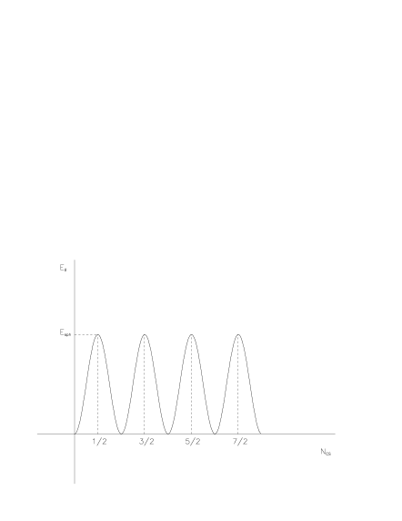
Figure 5: The potential energy of the $SU(2)$ gauge field as a function of the Chern–Simons number. The minima correspond to configurations with zero gauge field energy but different baryon number

Between the degenerate vacua there exist unstable, time–independent solutions of the field equations called sphalerons. The sphalerons were the first introduced by Klinkhamer and Manton Klinkhamer:1984di and they have Chern–Simons numbers $N_{CS}=1/2,3/2....$ At these saddle points the height of the barrier separating topologically distinct vacua has been estimated in the range

$$E_{sph}=\frac{2M_{W}}{a_{w}}B(\lambda/g^{2})=8-14\,\textrm{GeV}$$ (53)

for $\lambda$ varying from zero to infinity.

It is very significant that this non–trivial vacuum topology is related to the anomaly equation. The total baryon number is given by

$$B=\int d^{3}xJ^{0}_{B}$$ (54)

and it can be shown that the baryon number change during any time interval is related to the Chern–Simons number through the equation

$$\Delta B=N_{F}\left[N_{CS}(t_{2})-N_{CS}(t_{1})\right]~{},$$ (55)

since the time component of $K^{\mu}$ in Eq. (48) is simply the Chern–Simons number $N_{CS}$. Therefore if the baryon number is not to be conserved it is related to a change in the Chern–Simons number of the $SU(2)$ gauge vacuum.

At zero temperatures or low densities a transition from one vacuum configuration to another can be achieved by quantum tunneling. In the computation of the transition rates, a classical solution of the equations of motion can be used which is called an instanton. The instantons correspond to the classical solutions used in the WKB method of quantum mechanics McLerran:1992sg ; Coleman:1988 ; Weinberg:hc . The transition rates have been computed by t’Hooft 'tHooft:up ; 'tHooft:fv , but as it was shown these are suppressed by a semiclassical factor $\exp(-4\pi/a_{W})\sim 10^{-150}$. At zero temperature therefore baryon number non conservation is negligible. This of course is a consequence of the very large energetic barrier $(\sim 10\,\textrm{GeV})$ separating the vacua of different baryon number due to the sphaleron but fortunately this picture is completely different at high temperatures.

III.2.2 Nonzero Temperature

At finite temperatures thermal fluctuations with an energy higher than the height of the barrier between the two degenerate minima can classically traverse the maximum and enter the new minimum, leading to unsuppressed baryon number violation. The rate of penetration of the sphaleron barrier is then given by the Boltzmann factor associated with the formation of the sphaleron

$$\Gamma=(\alpha_{W}T)^{4}\exp[-E_{sph}(T)/T]~{},$$ (56)

where the sphaleron energy at temperature $T$ is given by

$$E_{sph}\sim B\frac{M_{W}(T)}{\alpha_{W}}~{}.$$ (57)

The factor $B$ is obtained numerically by solving the field equations. Such a numerical solution is still lacking, however we can expect that for temperatures larger than the $W$ boson mass, the baryon violation rate should behave like

$$\Gamma\sim\alpha_{W}T^{4}~{},$$ (58)

due to the vanishing of masses at high temperatures. This of course leads to a completely unsuppressed rate of baryon number violation. In particular this means that any pre–existing baryon asymmetry generated during the GUTs phase transition, would have disappeared until the time when the EW phase transition takes place. However these processes only violate $B+L$ since as we have seen $B-L$ does not have an anomaly and is exactly conserved in the standard model. Therefore a $B-L$ excess produced in the early universe will not be washed away.

It is very significant the role played by the sphaleron after the completion of the electroweak phase transition Turok:1992ar ; Turok:1990in . The sphaleron mass, which is proportional to the Higgs vacuum expectation value $\sigma(T_{c})$, must be large enough to strongly suppress baryon number violating processes. Otherwise, these processes may erase any asymmetry produced during the phase transition. For baryons to survive we need the sphaleron rate to be much less than the expansion rate of the universe. These considerations impose the constraint

$$\sigma(T_{c})/T_{c}\geq 1~{},$$ (59)

where $T_{c}$ is the temperature immediately after the transition and can also be used in order one to obtain an upper bound for the Higgs mass, which has found to be $m_{H}\leq 45\,\textrm{GeV}$ Shaposhnikov:tw ; Shaposhnikov:1987pf ; Bochkarev:1990gb .

III.3 $CP$ Violation

It has been well understood that $C$ and $CP$ violation is a crucial feature of any theory that attempts to explain the observed asymmetry between matter and antimatter in the universe starting from initially symmetric conditions. $CP$ symmetry requires that the partial rates of $CP$–conjugate processes be equal, therefore for any process that violates the baryon number there would be a $CP$–conjugate process of equal rate and no asymmetry could be generated. So far the Kaon system has been the only laboratory for the observation of $CP$ violation.

Violation of $C$ symmetry is a generic feature in the standard model of electroweak interactions, since due to the chiral nature of the $SU(2)$ gauge interaction, left and right chiralities of quarks have different interactions, so the Lagrangian of standard model has both $C$–even and $C$–odd pieces.

The standard model with two fermion families and a single Higgs doublet is a $CP$ invariant theory, but addition of the third generation violates the $CP$ invariance of the Lagrangian. As we referred in the second chapter on the formulation of the minimal standard model with one Higgs doublet, $CP$ violation in the model originates from the Cabbibo–Kobayashi–Maskawa (CKM) matrix which relates the quark mass eigenstates to the weak eigenstates.

The Yukawa term of the standard model Lagrangian involving the quark interactions with the scalar doublet was given in Eq. (32), but in terms of fields which are eigenstates of the weak interactions, can be written in the form

$${\cal L}_{Y}=\frac{g_{W}}{\sqrt{2}M_{W}}=\left[\overline{Q}_{L}KM_{d}d_{R}\Phi\overline{Q}_{L}KM_{u}u_{R}\tilde{\Phi}+\;h.c.\right]~{},$$ (60)

where $K$ is the CKM matrix which relates the two set of eigenstates and $M_{u}$, $M_{d}$ are the diagonal mass matrices of the quarks with charges 2/3 and $-1/3$ respectively. The specific form of the CKM matrix can be found in Hikasa:je .

For three fermion generations the CKM matrix must be $3\times 3$ and unitary and this constraint provides relationships between its elements, so finally its parameterisation can be done through three rotation angles and there can be only a physically meaningful phase which leads to observable $CP$ violation effects Farrar:hn ; Shaposhnikov:1991cu ; Jarlskog:jb . This $CP$ violation can be quantified through the combination Jarlskog:1985ht

$$\Delta_{CP} = \sin\,\theta_{12}\;\sin\,\theta_{23}\;\sin\,\theta_{13}\;\sin\,\delta_{CP}$$ (61)

$$\times(m_{t}^{2}-m_{c}^{2})(m_{t}^{2}-m_{u}^{2})(m_{c}^{2}-m_{u}^{2})$$

$$\times(m_{d}^{2}-m_{s}^{2})(m_{b}^{2}-m_{d}^{2})(m_{s}^{2}-m_{d}^{2})~{},$$

where $\theta_{ij},\;i,j=1,2,3$ are real angles and the phase $\delta_{CP}$ lies in the range $0\leq\delta_{CP}\leq 2\pi$. In order to get nonzero $CP$ violation, the quark mass matrices must have non-degenerate elements and also $\theta_{ij}\neq 0,\pi,\;i,j=1,2,3$, while $\delta_{CP}\neq 0,\pi$.

According to the analysis by Shaposhnikov Shaposhnikov:1991cu , the strength of the $CP$ violation in the standard electroweak model even at high temperatures appears to be too small, so it is unlikely that it can explain the observed baryon asymmetry. This conclusion results from arguing that the only natural scale for the baryogenesis problem is the temperature of the electroweak phase transition, which as we show in the Section V is of an order $T\sim 100\,\textrm{GeV}$. At this temperature the Yukawa interaction can be treated as a perturbation, because the quark masses are small compared with the temperature. The baryon asymmetry as defined in Section I is a dimensionless number, so to get an estimation of the asymmetry, the quantity given by Eq. (61) should be divided by something with dimensions of $(mass)^{12}$ and a natural choice is the temperature itself Farrar:hn . Hence,

$$\frac{n_{B}}{s}\leq\frac{\Delta_{CP}}{N_{eff}T^{12}}\sim 10^{-20}~{},$$ (62)

where $N_{eff}$ is the number of degrees of freedom in the standard model.

The same author suggested in subsequent work Shaposhnikov:tw ; Shaposhnikov:1987pf a possible way out of this problem. He assumed that accumulation of small $CP$ violating effects during the expansion of the universe could enhance the total $CP$ violation during the electroweak phase transition, but this result is not acceptable in general. Recent investigations show that the most promising models are models with enhanced the scalar sector and in particular the models with two scalar Higgs doublets Cohen:1991iu .

IV The Effective Potential

IV.1 Introduction

At the very early stages of its evolution the universe is filled with matter at very high energies and densities, so matter should be described in terms of quantum fields. In order to investigate how the electroweak phase transition could have occurred at the beginning of the universe we need to work in the framework of quantum field theory. The basic tool for the investigation of the nature of the electroweak phase transition is the effective potential, the quantity which has the meaning of the potential energy density of the system under consideration.

The discussion on spontaneous symmetry breaking in Section II.3 was purely classical. The particle spectrum was determined by minimization of the classical potential $V_{0}(\phi)$ as it appears into the Lagrangian and describes the potential energy density of a constant scalar field. The effective potential has also the meaning of a potential energy density. A quantum field theory involves virtual particles, which affect the field energy density through emission and reabsorption processes. This generalization of the classical potential to include the quantum corrections is known as the effective potential. Minimization of the effective potential gives the field configuration with the minimal energy, the vacuum of the theory.

Proceeding further, analysis of matter behaviour at non zero temperatures involves thermal fluctuations of the fields that one should take into account. Thus, a generalization of the effective potential at finite temperature is needed, for the inclusion of temperature dependent quantum effects. As it will be clear in what follows from the mathematical definition the effective action has the meaning of the free energy of the quantum system under consideration. The finite temperature effective potential $V(\phi,T)$ as Linde states Linde:1990 at its extrema coincides with the free energy density.

The effective potential has been studied extensively in the literature. An elegant discussion on the physical meaning of the effective potential and its calculation is explored by Coleman Coleman:1988 . A detailed analysis of the theory of the effective potential at zero and finite temperature with applications on cosmological models is given by Brandenberger Brandenberger:cz . The electroweak Higgs potential for the standard model and its extensions has been investigated by Sher Sher:1988mj . Early discussions on the subject are those of Coleman and Weinberg Coleman:jx involving calculation of the effective potential for a general gauge theory at zero temperature. Generalization of the effective potential at finite temperature is given by Dolan and Jackiw Dolan:qd and Linde Linde:1990 ; Linde:px . In what follows we give a formal discussion on the notion of the effective potential as it appears in the framework of quantum field theory.

The outline of this section is as follows: In Section IV.2 we discuss the properties of the effective potential at zero temperature and give the basic steps for its calculation in the framework of quantum field theory, using the path integral formalism. For this analysis we restrict ourselves to the one loop radiative corrections. In Section IV.3 we generalize the idea of the effective potential at finite temperature. This generalization appears in a form of integral terms which we add to the zero temperature effective potential. At high temperatures these integrals can be approximated expanding them in a series. The high temperature approximation of the fermion and boson contribution to the effective potential is compared with the exact calculation of the one loop radiative correction integrals using numerical methods.

IV.2 Zero Temperature Effects

IV.2.1 Path Integral Formalism

The effective potential can be calculated in an elegant way using the path integral formalism and the notion of generating functionals. Consider the case of a real scalar field and suppose that an external c–number source $J(x)$, a function of space and time, is added into the Lagrangian coupled linearly to the field $\phi$. Then the transition amplitude from the vacuum state in the far past to the vacuum state in the far future is defined as

$$Z[J]=\int\mathcal{D}\phi\exp(i\int d^{4}x[\mathcal{L}(\phi)+J(x)\phi(x)])~{}.$$ (63)

This amplitude can be expanded in a functional Taylor series in terms of the source $J(x)$, with coefficients $G_{u}^{n}(x_{1},x_{2},\ldots,x_{n})$ the Green functions of the theory. These Green functions can be found by functional differentiation of $Z[J]$ with respect to $J(x)$, at $J(x)=0$.

One can introduce the generating functional of the connected Green functions $W[J]$, which is related to $Z[J]$ by

$$Z[J]=\exp(iW[J])~{}.$$ (64)

Expanding this functional in powers of $J(x)$, the coefficients $G_{c}^{n}(x_{1},x_{2},\ldots,x_{n})$ are the connected Green’s functions. The connected Green’s functions $G^{(n)}_{c}$ are given by the functional derivative of $W[J]$ with respect to $J(x)$, at $J(x)=0$.

At this point we have to introduce a quantity which is referred as the classical field $\phi_{c}(x)$. This is a functional of the source $J(x)$ and is defined as the vacuum expectation value of the field operator in the presence of the source as

$$\phi_{c}(x)=\frac{\delta W[J]}{\delta J(x)}~{}.$$ (65)

In the absence of the source, the classical field $\phi_{c}(x)$ is just the vacuum expectation value of the field operator.

The generating functional of the 1PI (one particle irreducible) Green functions is called the effective action and is defined by the functional Legendre transform

$$\Gamma[\phi_{c}]=W[J]-\int d^{4}xJ(x)\phi_{c}(x)~{}.$$ (66)

It is called the effective action, because it is a functional of the classical field $\phi_{c}$ and hence akin to the classical action $S[\phi]$. From the definition of the effective action, it follows that the source can be obtained in the form of a functional derivative as

$$\frac{\delta\Gamma[\phi_{c}]}{\delta\phi_{c}(x)}=-J(x)~{}.$$ (67)

The effective action can be expanded in powers of $\phi_{c}$, or alternatively one can expand about a constant value of the field $\phi_{c}$. This is the same as expanding in powers of the derivatives of $\phi_{c}$. Thus in position space it is an expansion of the type

$$\Gamma[\phi_{c}]=\int d^{4}x[-V(\phi_{c})+\frac{1}{2}(\partial_{\mu}\phi_{c})^{2}Z(\phi_{c})+\ldots]~{},$$ (68)

where $V(\phi_{c})$ and $Z(\phi_{c})$ are ordinary functions of $\phi_{c}$ , not functionals, and the function $V(\phi_{c})$ is known as the effective potential. In the case of a classical field $\phi_{c}$ which is constant in space and time and in the absence of the source $J$, $\phi_{c}$ has the significance of the vacuum expectation value (VEV) of the field operator

$$\frac{dV(\phi_{c})}{d\phi_{c}}=0~{}.$$ (69)

This last equation allows one to interpret the VEV of the field operator as the stationary point of the effective potential, which can be obtained by solving the above equation. Of course, in the case when the field is to vary in space or time, we have to solve the more general equation $\delta\Gamma/\delta\phi_{c}=0$. Thus the VEV of the field operator, taking into account quantum corrections, can be found by minimizing the effective potential. If the effective potential has several local minima, it is the absolute minimum that corresponds to the true ground state.

It is useful to see that the effective potential can be obtained as the infinite sum of the 1PI graphs with vanishing external momenta Coleman:jx , although we will not make use of this method in order to evaluate that in the case of the scalar field. One can expand the effective action functionally in terms of $\phi_{c}$ as

$$\Gamma[\phi_{c}] = \sum_{n=1}^{\infty}\frac{1}{n!}\int d^{4}x_{1}\ldots d^{4}x_{n}\;\phi_{c}(x_{1})\ldots\phi_{c}(x_{n})$$ (70)

$$\times\Gamma^{(n)}(x_{1},\ldots,x_{n})~{}.$$

The coefficients $\Gamma^{(n)}$ are referred as the one–particle–irreducible (1PI) Green functions. Fourier transforming the 1PI Green functions to momentum space, the expression for the effective action takes the form

$$\Gamma[\phi_{c}] = \sum_{n=1}^{\infty}\frac{1}{n!}\int d^{4}p_{1}\ldots d^{4}p_{n}\;\delta^{4}(p_{1}+\ldots+p_{n})$$ (71)

$$\times\Gamma^{(n)}(p_{1},\ldots,p_{n})\;\tilde{\phi_{c}}(p_{1})\ldots\tilde{\phi_{c}}(p_{n})~{},$$

where $\tilde{\phi_{c}}(p_{i})$ is the Fourier transform of $\phi_{c}$. Thus, comparing this last expression with the momentum space expansion of the effective action above, we find that the effective potential is given as a sum of the 1PI graphs of the form

$$V(\phi_{c})=-\sum_{n=1}^{\infty}\frac{1}{n!}\Gamma^{(n)}(p_{i}=0)\;\phi^{n}_{c}~{}.$$ (72)

IV.2.2 Scalar Loops

In order to understand how the effective potential is calculated, we present here the evaluation of the effective potential for a theory involving a real scalar field with quartic self interaction. The Lagrangian governing this theory is given by

$$\mathcal{L}=\frac{1}{2}(\partial_{\mu}\phi)^{2}+\frac{1}{2}\mu^{2}\phi^{2}-\frac{1}{4}\lambda\phi^{4}~{}.$$ (73)

The potential energy density of the real scalar field at classical level, which is commonly called the classical potential and denoted by $V_{0}(\phi)$, is given by

$$V_{0}(\phi)=-\frac{1}{2}\mu^{2}\phi^{2}+\frac{1}{4}\lambda\phi^{4}~{},$$ (74)

where the field mass squared $\mu^{2}$ and the coupling constant $\lambda$ are positive. The effective potential which is usually denoted by $V(\phi)$ will result in as a sum of the classical potential, plus terms due to radiative corrections Itzykson:rh ; Bailin:wt ; Ryder:wq ; Ramond:pw ; Rivers:hi .

As it was referred earlier the diagrammatic method of summing the 1PI graphs can be used for the calculation of the effective potential, however we present here an alternative method which is based on the saddle point evaluation of path integrals Ryder:wq ; Ramond:pw . According to this method exponential integrals involving a function $f(x)$ which is stationary at some point $x_{0}$, can be solved by expanding $f(x)$ about this point. Then, omitting higher derivatives, the integral becomes a Gaussian and thus can be evaluated according to standard methods.

The starting point is the generating functional of the connected Green’s functions, where we have restored the Planck’s constant so it takes the form

$$\exp\bigg{(}\frac{i}{\hbar}W[J]\bigg{)}=\mathcal{N}\int\mathcal{D}\phi\exp\bigg{(}\frac{i}{\hbar}S[\phi,J]\bigg{)}$$ (75)

and the normalization constant $\cal N$ is chosen such as $W[0]=1$. Although in natural units the Planck constant is equal to unity, we restore it here in order to get an expansion in terms of $\hbar$ and make clear that we calculate quantum corrections to the classical potential. The powers of $\hbar$ count the number of the closed loops in the loop expansion. The action $S[\phi,J]$ in presence of the source $J(x)$ is given by

$$S[\phi,J]=\int d^{4}x[\mathcal{L}(\phi(x))+J(x)\phi(x)]~{}.$$ (76)

The saddle point is at $\phi=\phi_{0}$ and satisfies

$$\frac{\delta S[\phi,J]}{\delta\phi(x)}\bigg{|}_{\phi=\phi_{0}}=\hbar J(x)~{},$$ (77)

where $\phi$ is a function of $x$ and also a functional of $J$. In the case when the source $J$ tends to zero, $\phi_{0}(x)$ becomes a solution to the classical equations of motion. Expanding the action $S[\phi,J]$ about the stationary point at $\phi=\phi_{0}$ yields

$$S[\phi,J] = S[\phi_{0},J]+\int dx[\phi(x)-\phi_{0}]S^{\prime}[\phi_{0},J]$$

$$\mbox{}+\frac{1}{2}\int dxdy[\phi(x)-\phi_{0}][\phi(y)-\phi_{0}]S^{\prime\prime}[\phi_{0},J]~{},$$

plus higher order terms which we omit, since we are interested in calculating radiative corrections up to one loop only. In this last equation we have used the shorthand

$$S^{\prime}[\phi_{0},J]=\frac{\delta S}{\delta\phi(x)}\bigg{|}_{\phi=\phi_{0}}~{},$$

$$S^{\prime\prime}[\phi_{0},J]=\frac{\delta^{2}S}{\delta\phi(x)\delta\phi(y)}\bigg{|}_{\phi=\phi_{0}}~{}.$$

We then differentiate functionally the action and insert the result into the equation above. The resulting integral is a Gaussian one, so going over to Euclidean space we get finally the loop expansion for $W[J]$, ignoring correction terms of order $\hbar^{2}$ and higher,

$$W[J]=S[\phi_{0}]+\hbar\int dx\phi_{0}(x)J(x)+\frac{i\hbar}{2}\textrm{Tr}\ln[\Box+V_{0}^{\prime\prime}(\phi_{0})]~{}.$$ (78)

Inserting this expression into the defining equation of the effective action we get, by putting the source $J\rightarrow 0$,

$$\Gamma[\phi_{c}]=S[\phi_{c}]+\frac{i\hbar}{2}\textrm{Tr}\ln[\Box+V_{0}^{\prime\prime}(\phi_{0})]~{}.$$ (79)

For a field which is constant in space and time, through the expansion of the effective action we find for the effective potential the expression

$$V(\phi)=V_{0}(\phi)+\frac{\hbar}{2}\int\frac{dk^{4}_{E}}{(2\pi)^{4}}\ln[k^{2}_{E}+V_{0}^{\prime\prime}(\phi)]~{},$$ (80)

where in the final step we have used that the trace of an operator is the sum over its eigenvalues and we expressed the result on going over to Euclidean momentum space.

IV.2.3 Renormalization

The above integral is divergent as it happens in general when one calculates radiative corrections involving integrations over the internal momenta of the graphs. For the theory to be renormalized, the divergences must be absorbed, if possible, into the parameters of the theory. In order to evaluate this integral we introduce a cut–off at some large momentum $k^{2}=\Lambda^{2}$, so we obtain

$$V_{1}(\phi) = V_{0}(\phi)+\frac{\Lambda^{2}}{32\pi^{2}}m^{2}(\phi)$$ (81)

$$+\frac{m^{4}(\phi)}{64\pi^{2}}\bigg{[}\ln\bigg{(}\frac{m^{2}(\phi)}{\Lambda^{2}}\bigg{)}-\frac{1}{2}\bigg{]}+V_{ct}(\phi)~{},$$

where the field dependent squared mass of the scalar $m(\phi)$ is defined as the second derivative of the classical potential as

$$m^{2}(\phi)=\frac{d^{2}V_{0}(\phi)}{d\phi^{2}}=3\lambda\phi^{2}-\mu^{2}.$$ (82)

To remove the cut–off dependence we have introduced a counterterm potential which has the same structure as the original potential

$$V_{ct}(\phi)=\frac{1}{2}A\phi^{2}+\frac{1}{4}B\phi^{4}+C~{}.$$ (83)

We can determine the coefficients $A$ and $B$ by requiring that the position of the minimum of the effective potential and the Higgs field mass remain in their classical values Linde:1990 ; Linde:px , so

$$\frac{dV_{1}(\phi)}{d\phi}\bigg{|}_{\phi_{c}=\sigma}=0$$ (84)

and the Higgs field mass $m^{2}_{H}=2\mu^{2}$ results as the second derivative of the potential evaluated at $\phi_{c}=\sigma$,

$$\frac{dV^{2}_{1}(\phi)}{d\phi^{2}}\bigg{|}_{\phi_{c}=\sigma}=2\mu^{2}~{}.$$ (85)

The final expression of the effective potential for the real scalar field, including radiative corrections up to one loop, takes the form

$$V_{1}(\phi) = V_{0}(\phi)+\frac{m^{4}(\phi)}{64\pi^{2}}\ln\bigg{(}\frac{m^{2}(\phi)}{m^{2}(\sigma)}\bigg{)}$$ (86)

$$-\frac{1}{32\pi^{2}}m^{2}(\phi)m^{2}(\sigma)-\frac{3}{128\pi^{2}}m^{4}(\phi)~{},$$

where $V_{0}(\phi)$ is the classical potential. Other renormalization conditions can also be introduced Coleman:jx ; Sher:1988mj but the physical results are meant to be the same.

IV.2.4 Fermion and Boson Loops

The saddle point evaluation of the one loop corrections to the effective potential was an elegant way to obtain the effective potential in the case of the one scalar field. In order to proceed and obtain an expression of the effective potential for the standard electroweak model we need to know the one loop contributions of fermions and vector bosons. The case of a general non-abelian gauge theory was the first discussed by Coleman and Weinberg Coleman:jx . An analytic presentation of the subject is also given by Rivers Rivers:hi and Sher Sher:1988mj . In this general case it is more convenient to revert to the definition of the effective potential from the expansion of the effective action and the first step is to extend the scalar sector including more fields. A different approach, based on the evaluation of Gaussian integrals as in the case of the scalar field, is given in Bailin and Love Bailin:wt .

According to Anderson and Hall Anderson:1991zb , the analysis given in the above references can be summarized into that the unrenormalized one loop self–energy contribution of virtual particles, adds to the classical potential a term which in the case of fermions is given by

$$\Delta V_{1f}(\phi) = -\frac{1}{64\pi^{2}}m^{4}_{f}(\phi)\ln\bigg{(}\frac{m^{2}_{f}(\phi)}{\Lambda^{2}}\bigg{)}$$ (87)

$$+\frac{1}{128\pi^{2}}m^{4}_{f}(\phi)-\frac{1}{32\pi^{2}}m^{4}_{f}(\phi)\Lambda^{2}$$

for each fermionic degree of freedom. On the other hand the bosons contribution has a similar form, except the opposite sign, and is given by

$$\Delta V_{1b}(\phi) = \frac{1}{64\pi^{2}}m^{4}_{b}(\phi)\ln\bigg{(}\frac{m^{2}_{b}(\phi)}{\Lambda^{2}}\bigg{)}$$ (88)

$$-\frac{1}{128\pi^{2}}m^{4}_{b}(\phi)-\frac{1}{32\pi^{2}}m^{2}_{b}(\phi)\Lambda^{2}~{}.$$

In both the above equations $\Lambda$ is a cut–off which has been introduced in order to evaluate the divergent integrals.

Summarizing the above discussion, the one loop effective potential in the case of a general gauge theory involving fermion, scalar and boson fields can be written in the general form

$$V_{1}(\phi)=V_{0}(\phi)+\Delta V_{1}(\phi)+V_{ct}(\phi)~{},$$ (89)

where $\Delta V_{1}(\phi)$ is the sum of fermions, scalars and bosons one loop contributions to the effective potential and $V_{ct}(\phi)$ is a counterterm potential which is used to remove the cut–off dependence as in the scalar field case. We adopt the same renormalization condition as before in order to retain the Higgs mass and the position of the minimum of the potential for each degree of freedom to which the scalar couples, so for the bosons we have a contribution of the form

$$\Delta V_{1b} = \sum_{b}\frac{n_{b}}{64\pi^{2}}\bigg{[}m^{4}_{b}(\phi)\ln\bigg{(}\frac{m^{2}_{b}(\phi)}{m^{2}_{b}(\sigma)}\bigg{)}-\frac{3}{2}m^{4}_{b}(\phi)$$ (90)

$$+2m^{2}_{b}(\phi)m^{2}_{b}(\sigma)\bigg{]}~{},$$

while for the fermions the contribution reads as

$$\Delta V_{1f} = -\sum_{f}\frac{n_{f}}{64\pi^{2}}\bigg{[}m^{4}_{f}(\phi)\ln\bigg{(}\frac{m^{4}_{f}(\phi)}{m^{2}_{f}(\sigma)}\bigg{)}-\frac{3}{2}m^{4}_{f}(\phi)$$ (91)

$$+2m^{2}_{f}(\phi)m^{2}_{f}(\sigma)\bigg{]}~{},$$

where $n_{b}$ and $n_{f}$ are the numbers of degrees of freedom associated to spin, particle–antiparticle states and internal symmetries (coloured quark states).

IV.3 Finite Temperature Effects

IV.3.1 Fields at Finite Temperature

In order to investigate the electroweak phase transition in the next section, we need a generalization of the effective potential at finite temperatures. We present here how the notion of the effective potential can be generalized at finite temperature, following the ideas of Dolan and Jackiw Dolan:qd , Linde Linde:1990 ; Linde:px and Sher Sher:1988mj .

At finite temperature a field theory is equivalent to an ensemble of finite temperature Green functions. The average value of an operator at nonzero temperature is defined by the Gibbs average as

$$\mathcal{O}(x_{1},x_{2},\ldots,x_{n})=\frac{\textrm{Tr}e^{-\beta H}\mathcal{O}(x_{1},x_{2}\ldots,x_{n})}{\textrm{Tr}e^{-\beta H}}~{},$$ (92)

where $H$ is the Hamiltonian of the system under consideration and $\beta=1/k_{B}T=1/T$, since for the sake of simplicity the Boltzmann’s constant $k_{B}$ can be taken equal to unity. Then, according to the proof given by Sher Sher:1988mj , Green’s functions at non zero temperature obey the same equations as those at zero temperature, but under different boundary conditions. The finite temperature Green’s functions concerning bosons are periodic in Euclidean time, $\tau\equiv it$, with a period $\beta=1/T$, instead of having the usual boundary conditions $t=\pm\infty$. On the other hand fermionic finite temperature Green’s functions obey antiperiodic boundary conditions with the same period $\beta$.

In analogy with the previous section the finite temperature effective potential can be calculated by using similar methods as in zero temperature field theory and the path integral formalism. A finite temperature effective action $\Gamma^{\beta}[\phi_{c}]$ is defined by analogy to that at zero temperature, since the vacuum expectation value of the classical field at zero temperature now corresponds to a thermodynamic average. The finite temperature effective potential may be defined by an expansion of the effective action analogous to that of the previous section and its calculation proceeds through the evaluation of Gaussian path integrals at Euclidean space–time. The only difference in these calculations is that when one calculates integrals involving boson fields all the boson momenta $k_{0}$ should be replaced by the Matsubara frequencies for bosons $2\pi nT$ with $n$ an integer. On the other hand, since fermionic fields are antiperiodic, the corresponding fermion momentum $k_{0}$ must be replaced by $(2n+1)\pi T$. So finally, instead of integrating over $k_{0}$, one has to sum over $n$. We show this calculation in some detail and give relevant references in the following sections.

IV.3.2 Scalar Fields at Finite Temperature

Consider first the case of a scalar field. We have to expand the Lagrangian around a constant field $\phi_{c}$. The field dependent mass squared, which is called the effective mass, is given by

$$m^{2}(\phi_{c})=3\lambda\phi_{c}^{2}-\mu^{2}~{}.$$ (93)

The zero loop effective potential, the so–called classical potential, is temperature independent and is given by

$$V_{0}(\phi_{c})=-\frac{1}{2}\mu^{2}\phi_{c}^{2}+\frac{1}{4}\lambda\phi^{4}_{c}~{}.$$ (94)

We have already calculated the one loop approximation to the effective potential at zero temperature as

$$V^{0}_{1s}(\phi_{c})=\frac{1}{2}\int\frac{d^{4}k}{(2\pi)^{4}}\ln[k^{2}+m^{2}(\phi_{c})]~{}.$$ (95)

At finite temperature the above expression, as we have stated earlier, one has to replace the scalar boson momenta $k_{0}$ by the Matsubara frequency $2\pi nT$, so it becomes

$$V^{T}_{1s}(\phi_{c})=\frac{1}{2}T\sum_{n=-\infty}^{\infty}\int\frac{d^{3}\textbf{k}}{(2\pi)^{3}}\ln[\textbf{k}^{2}+(2\pi nT)^{2}+m^{2}(\phi_{c})]~{}.$$ (96)

The sum over $n$ diverges, so in order to evaluate this integral one can follow the procedure given by Dolan and Jackiw Dolan:qd . The result splits in two parts, one temperature independent part

$$V^{0}_{1s}(\phi_{c})=\int\frac{d^{3}\textbf{k}}{(2\pi)^{3}}\frac{\sqrt{\textbf{k}^{2}+m^{2}(\phi_{c})}}{2}~{},$$ (97)

which is equivalent to the one loop effective potential at zero temperature which we have calculated in the previous section, and a temperature dependent part

$$V^{T}_{1s}(\phi,T)=\frac{T^{4}}{2\pi^{2}}\int_{0}^{\infty}dx\,x^{2}\ln[1-\exp(-A(x,m,T))]~{}.$$ (98)

In this last equation we have introduced the shorthand expression $A(x,m,T)=\sqrt{x^{2}+m^{2}(\phi_{c})/T^{2}}$ . These final steps are explained in some detail in the next section where we give the basic steps for the calculation of the finite temperature effective potential for a general gauge theory.

Thus summarizing the above discussion, the finite temperature effective potential for a real scalar field including the one loop radiative corrections can be written as

$$V_{1s}(\phi,T)=V_{0}(\phi)+V_{1s}^{0}(\phi)+V_{1s}^{T}(\phi,T)~{}.$$ (99)

The finite temperature contribution vanishes as it should at zero temperature $T=0$, when the mass squared $m^{2}(\phi_{c})$ is positive. But as it was stressed by Dolan and Jackiw Dolan:qd , if one is to use this full expression of the one loop potential, there are some serious difficulties for small values of the field, $\phi^{2}<\mu^{2}/3\lambda$, since the mass squared of the Higgs scalar becomes negative leading to an unacceptable complex one loop effective potential.

Fortunately in the case of the minimal standard model, which we discuss in the next section, the scalar loops can be safely ignored, since they are negligible as compared to fermion and vector boson contributions, simply because there is a large degeneracy factor associated to the latter, while there is only one Higgs scalar.

IV.3.3 Fermions–Bosons at Finite Temperature

The above discussion can be applied to a general gauge theory and as we stated earlier there is an analogy between the computation of the effective potential at finite temperature to that at zero temperature. We have to expand the scalar fields around their expectation values, which are now thermal averages, and isolate the terms in the Lagrangian which are quadratic in all the fields. Then the one loop contribution to the effective action is obtained as a Gaussian path integral. Suppose we deal with a general gauge theory involving fermions, scalars, gauge bosons and Fadeev–Popov ghost fields. We insert the quadratic Lagrangian into the expression of the effective action and evaluating the resulting Gaussian integrals, the finite temperature effective potential results as a sum of traces of the form Bailin:wt

$$-\int_{0}^{\beta}d\tau\int d^{3}xV^{T}_{1}(\phi_{c})=-\frac{1}{2}\textrm{Tr}\ln\textbf{A}-\frac{1}{2}\textrm{Tr}\ln\textbf{B}+\textrm{Tr}\ln\textbf{C}~{}.$$ (100)

The scalar contribution is given by the first trace

$$\textrm{Tr}\ln\textbf{A}=\int d^{3}x\sum_{i}^{\textrm{scalar}}\int\frac{d^{3}\textbf{k}}{(2\pi)^{3}}\sum_{n}\ln[\omega^{2}_{n}+\textbf{k}^{2}+(m^{2}_{s})_{i}]~{},$$ (101)

where $m_{s}^{2}=m_{s}^{2}(\phi_{c})$ are the eigenvalues of the scalar mass matrix. The contribution of the vector bosons has the form

$$\textrm{Tr}\ln\textbf{B}=\int d^{3}x\sum^{\textrm{boson}}_{a}\int\frac{d^{3}\textbf{k}}{(2\pi)^{3}}\sum_{n}3\ln[\omega_{n}^{2}+\textbf{k}^{2}+(m_{b}^{2})_{a}]~{},$$ (102)

with $m_{b}^{2}=m_{b}^{2}(\phi_{c})$ being the eigenvalues of the vector boson mass matrix. In a similar way the fermion term appears as

$$\textrm{Tr}\ln\textbf{C}=2\int d^{3}x\sum_{r}^{\textrm{fermion}}\int\frac{d^{3}\textbf{k}}{(2\pi)^{3}}\sum_{n}\ln[\omega_{n}^{2}+\textbf{k}^{2}+(m^{2}_{f})_{r}]~{}.$$ (103)

These can be evaluated by using the Matsubara frequency sums which in the case of bosons is given by

$$\sum_{n}\ln(\omega_{n}^{2}+x^{2})=\beta x+2\ln(1-e^{-\beta x})$$ (104)

plus an $x$–independent constant. In the fermion case the relevant formula has a similar form apart from a minus sign,

$$\sum_{n}\ln(\omega_{n}^{2}+x^{2})=\beta x+2\ln(1+e^{-\beta x})~{},$$ (105)

where for the antiperiodic fermions $\omega_{n}=(2n+1)\pi T$.

After summing, the scalar contribution takes the form

$$\Delta V_{1s}(\phi_{c},T) = \frac{1}{2}\int\frac{d^{3}\textbf{k}}{(2\pi)^{3}}\sum_{i}\bigg{[}(E^{2}_{s})_{i}$$ (106)

$$+\frac{2}{\beta}\ln\big{[}1-\exp[-\beta(E^{2}_{s})_{i}]\big{]}\bigg{]}~{},$$

the vector bosons contribute the following term

$$\Delta V_{1b}(\phi_{c},T) = \frac{1}{2}\int\frac{d^{3}\textbf{k}}{(2\pi)^{3}}\sum_{a}\bigg{[}3(E^{2}_{b})_{a}$$ (107)

$$+\frac{6}{\beta}\ln\big{[}1-\exp[-\beta(E^{2}_{b})_{a}]\big{]}\bigg{]}~{},$$

and the contribution of the fermions reads as

$$\Delta V_{1f}(\phi_{c},T) = -2\int\frac{d^{3}\textbf{k}}{(2\pi)^{3}}\sum_{r}\bigg{[}(E^{2}_{f})_{r}$$ (108)

$$+\frac{2}{\beta}\ln\big{[}1+\exp[-\beta(E^{2}_{f})_{r}]\big{]}\bigg{]}~{},$$

where we have used that $E^{2}_{a}=\sqrt{\textbf{{k}}^{2}+m_{a}^{2}}$ for $a=s,b,f$ for scalars, boson and fermions. All the above equations can be separated into a part $\Delta V_{1i}^{0}(\phi),i=s,b,f$ which is temperature independent and a temperature dependent part $\Delta V_{1i}^{T}(\phi)$ for each of the above field contributions.

By using the fact that Dolan:qd ; Bailin:wt

$$\int\frac{d^{3}\textbf{k}}{(2\pi)^{3}}\sqrt{\textbf{k}^{2}+R}=\int\frac{d^{4}k}{(2\pi)^{4}}\ln(k_{0}^{2}+\textbf{k}^{2}+R)$$ (109)

plus a constant independent of $R$ and evaluating the integrals in the zero temperature part, we get the one loop quantum corrections which we have already calculated in the previous section. By setting $x\equiv|\textbf{k}|/T$ in the temperature dependent part of the above equations, the scalar field contribution to the effective potential at finite temperature takes the form

$$\Delta V^{T}_{1s}(\phi,T) = \frac{T^{4}}{2\pi^{2}}\int_{0}^{\infty}dx\;x^{2}$$

$$\times\sum_{i}\ln\big{[}1-\exp(-\sqrt{x^{2}+(m_{s}^{2})_{i}/T^{2}})\big{]}~{},$$

the boson term is

$$\Delta V^{T}_{1b}(\phi,T) = 3\frac{T^{4}}{2\pi^{2}}\int_{0}^{\infty}dx\;x^{2}$$

$$\times\sum_{a}\ln\big{[}1-\exp(-\sqrt{x^{2}+(m_{b}^{2})_{a}/T^{2}})\big{]}~{},$$

and the fermion term is

$$\Delta V^{T}_{1f}(\phi,T) = -4\frac{T^{4}}{2\pi^{2}}\int_{0}^{\infty}dx\;x^{2}$$

$$\times\sum_{r}\ln\big{[}1+\exp(-\sqrt{x^{2}+(m_{b}^{2})_{r}/T^{2}})\big{]}~{},$$

where $m_{i}=m_{i}(\phi_{c}),i=s,f,b$ are the scalar, fermion and boson mass eigenvalues.

It is easy to observe the similarity in the formulas between the vector bosons and scalars. The only difference is the factor 3 which appears in the boson case. This factor expresses the one longitudinal and the two transverse degrees of freedom of a massive vector boson. On the other hand the factor 4 in the formula for fermions corresponds to the two fermionic spin states times the two particle antiparticle states. On summarizing the above discussion we can say that finite temperature effects for bosons takes the form

$$\Delta V^{T}_{1b}(\phi,T) = \sum_{b}\frac{n_{b}T^{4}}{2\pi^{2}}\int_{0}^{\infty}dx\;x^{2}$$

$$\times\ln[1-\exp(-\sqrt{x^{2}+m_{b}^{2}(\phi)/T^{2}})]~{}.$$

The fermion term has a similar form apart from the positive sign in the argument of the logarithm and that their contribution has an overall minus sign, so

$$\Delta V^{T}_{1f}(\phi,T) = -\sum_{f}\frac{n_{f}T^{4}}{2\pi^{2}}\int_{0}^{\infty}dx\;x^{2}$$

$$\times\ln[1+\exp(-\sqrt{x^{2}+m_{f}^{2}(\phi)/T^{2}})]~{}.$$

As it was referred above for massive vector bosons the relevant factor which corresponds to the particle helicity states is $n_{b}=3$, since for fermions $n_{f}=4$. For coloured fermions, as it is the case of quarks, $n_{f}=12$.

IV.3.4 High Temperature Approximation

It is sometimes convenient to approximate the above integrals by using the high temperature expansion. When the temperature is high enough as compared to the particle masses the above integrals can be approximated by expanding them in a series in powers of $m(\phi)/T$. This expansion has been extensively used in the literature in investigations of the effective potential. The expansion of the integrals in the high temperature limit can be done by using the Riemann Zeta function Dolan:qd ; Kapusta:tk . According to the analysis given in the above references, the integral in the fermion case can be expanded as

$$\Delta V_{1f}^{HT}(\phi,T) = \sum_{f}n_{f}\bigg{[}-\frac{7\pi^{2}T^{4}}{720}+\frac{m^{2}_{f}T^{2}}{48}$$

$$+\frac{m_{f}^{4}}{64\pi^{2}}\ln\bigg{(}\frac{m_{f}^{2}}{c_{f}T^{2}}\bigg{)}+O\bigg{(}\frac{m_{f}^{6}}{T^{2}}\bigg{)}\bigg{]}~{},$$

where the constant $c_{f}$ is defined as $\ln c_{f}=\frac{3}{2}+2\ln\pi-2\gamma\approx 2.64$ and the Euler constant is $\gamma\approx 0.577$. The particle masses which appear in the above expression are field dependent, so $m_{f}=m_{f}(\phi)$.

Our aim was to verify the reliability of the high temperature expansion, so we have calculated the integrals given in the previous section numerically. For this calculation we have used a numerical code based on Simpson’s rule.

Figure 6: A fermion’s contribution to the effective potential as a function of $m_{f}(\phi)/T$. The solid line represents the exact calculation, while the dashed line corresponds to the high temperature expansion.

In order to compare a fermion’s contribution to the effective potential by using the high temperature approximation with the exact calculation of the integrals, the contribution of a fermionic degree of freedom to the free energy density (the effective potential) as a function of $m_{f}/T$ is given in Fig. 6. As we can observe in this figure, for $m_{f}/T<1.6$, the high temperature approximation is in good agreement (better than 5%) with the exact calculation of the effective potential.

In the boson case the expansion of the integral reads

$$\Delta V_{1b}^{HT}(\phi,T) = \sum_{b}n_{b}\bigg{[}-\frac{\pi^{2}T^{4}}{90}+\frac{m^{2}_{b}T^{2}}{24}$$

$$-\frac{m^{3}_{b}T}{12\pi}-\frac{m_{b}^{4}}{64\pi^{2}}\ln\bigg{(}\frac{m_{b}^{2}}{c_{b}T^{2}}\bigg{)}+O\bigg{(}\frac{m_{f}^{6}}{T^{2}}\bigg{)}\bigg{]}$$

where the constant $c_{b}$ is defined as $\ln c_{b}=\frac{3}{2}+2\ln 4\pi-2\gamma\approx 5.41$. As in the fermion case the boson masses are field dependent, so $m_{b}=m_{b}(\phi)$. The fermion and boson expressions look similar, but one can observe that there are no cubic terms in the formula for fermions since there cannot be modes of zero Matsubara frequency. This last observation turns to be very crucial in the standard model case which we investigate in the next section. A boson’s contribution to the effective potential is given in Fig. 7 and from this picture it is clear that the high temperature expansion of the integrals is consistent with the exact calculation to better than 5% for $m_{b}/T<2.2$. The previous graphs confirm similar results obtained by Anderson and Hall Anderson:1991zb .

Figure 7: A boson’s contribution to the effective potential as a function of $m_{b}(\phi)/T$. The solid line represents the exact calculation, while the dashed line corresponds to the high temperature expansion.

V Electroweak Phase Transition

V.1 Introduction

The third Sakharov condition, that the universe must be out of equilibrium, demands that the electroweak phase transition should be of the first order, if baryogenesis is to happen at this transition. Although the order of the transition is not yet completely established and the literature contains contradictory claims, most of the recent investigations suggest that it is of the first order. The basic tool for the investigation of the electroweak phase transition is the finite temperature effective potential. Our aim is to explore how the phase transition at the electroweak scale could have taken place and what is the order of the transition when the one loop approximation is used in the calculation of the effective potential.

In the next Section V.2 we use the analysis given in Section IV in order to calculate the one loop corrections to the effective potential of the standard model and obtain an expression of the effective potential in the high temperature approximation. In Section V.3 we investigate the nature the electroweak phase transition through the analysis of the evolution of the effective potential, while in Section V.4 we outline how the transition is dynamically achieved.

V.2 The Standard Model Effective Potential

V.2.1 Zero Temperature

The calculations concerning the contributions to the effective potential of fermions and bosons given in Section IV can be applied in the case of the minimal standard model of the electroweak interactions. The effective potential at zero temperature will appear as a sum of the classical potential $V_{0}(\phi)$ plus terms due to one loop radiative corrections of fermions and bosons which are present at the standard electroweak model and where we will assume that the contribution of the Higgs scalar is negligible.

Only the heaviest particles give a significant contribution to the effective potential so we have to include the three gauge bosons, the two charged $W$ and the neutral $Z$, since the only heavy fermion is the top quark. The top’s mass is not known experimentally but there is an experimental lower limit which is about $130\,\textrm{GeV}$ Abachi:1994je . By using the results of Section IV.2 the contribution of the two charged vector bosons takes the form

$$\Delta V_{1W}(\phi)=2\frac{3}{64\pi^{2}\sigma^{4}}m_{W}^{4}(\sigma)\left[\ln\bigg{(}\frac{\phi^{2}}{\sigma^{2}}\bigg{)}-\frac{3}{2}\phi^{4}+2\sigma^{2}\phi^{2}\right]$$ (110)

where the factor 2 stands for the two charged particles and 3 corresponds to the polarization degrees of freedom. In this equation we have expressed the Ws’ contribution as a function of the field and the masses of the particles are those at tree level given by $m_{W}^{2}(\sigma)=1/4g^{2}\sigma^{2}$. In a similar way the contribution of the one neutral $Z$ boson is

$$\Delta V_{1Z}(\phi)=\frac{3}{64\pi^{2}\sigma^{4}}m_{Z}^{4}(\sigma)\left[\ln\bigg{(}\frac{\phi^{2}}{\sigma^{2}}\bigg{)}-\frac{3}{2}\phi^{4}+2\sigma^{2}\phi^{2}\right]$$ (111)

and the $Z$ mass at the minimum of the potential is $m_{Z}^{2}(\sigma)=1/4(g^{2}+g^{\prime^{2}})^{2}\sigma^{2}$. The top quark contributes the following term

$$\Delta V_{1t}(\phi)=-4\frac{3}{64\pi^{2}\sigma^{4}}m_{t}^{4}(\sigma)\left[\ln\bigg{(}\frac{\phi^{2}}{\sigma^{2}}\bigg{)}-\frac{3}{2}\phi^{4}+2\sigma^{2}\phi^{2}\right]$$ (112)

with a tree level mass $m_{t}^{2}(\sigma)=1/2g^{2}_{t}\sigma^{2}$, where $g_{t}$ is the top quark Yukawa coupling and the overall factor 12 corresponds to the degrees of freedom of the coloured top quark.

Adding the above terms the final expression of the effective potential for the standard electroweak model including quantum corrections up to one loop can be written as

$$\Delta V_{1}^{0}(\phi)=V_{0}(\phi)+\Delta V_{1W}(\phi)+\Delta V_{1Z}(\phi)+\Delta V_{1t}(\phi)$$ (113)

and in terms of the order parameter $\phi$

$$\Delta V^{0}_{1}(\phi)=-\frac{1}{2}\mu^{2}\phi^{2}+\frac{1}{4}\lambda\phi^{4}+2B\sigma^{2}\phi^{2}-\frac{3}{2}B\phi^{4}+B\phi^{4}\ln\frac{\phi^{2}}{\sigma^{2}}$$ (114)

where $B$ is defined as

$$B=\frac{3}{64\pi^{2}\sigma^{4}}(2m_{W}^{4}+m_{Z}^{4}-4m_{t}^{4})$$ (115)

and $\sigma=246\,\textrm{GeV}$ is the value of the scalar field at the minimum of the one loop potential $V^{0}_{1}(\phi)$ at zero temperature. The Higgs field coupling constant is defined as $\lambda=\mu^{2}/\sigma^{2}$ and the Higgs boson mass is given by $m_{H}^{2}=2\mu^{2}$. The masses of the particles which appear into the above expression for $B$ are the tree level masses, $m_{i}=m_{i}(\sigma),i=W,Z,t$. Similar expressions up to a change of variables appear also in references Carrington:1991hz ; Espinosa:1992gq ; Anderson:1991zb ; Dine:1991ck

V.2.2 Finite Temperature

At finite temperature we use the results of Section IV.3 and we add to the potential a term which includes the temperature induced effects. As we have discussed already only the heaviest particles give a significant contribution so we have to include only the two vector bosons and the top quark. As we stated earlier the scalar contribution can be ignored. We can write the finite temperature term in a compact form as

$$\Delta V_{1}^{T}(\phi,T)=\frac{T^{4}}{2\pi^{2}}[n_{W}J_{b}(y_{W})+n_{Z}J_{b}(y_{Z})-n_{t}J_{f}(y_{t})]$$ (116)

where $J_{b}(y)$ is the integral contribution of the bosons and is given by

$$J_{b}(y)=\int_{0}^{\infty}dxx^{2}\ln[1-\exp(-\sqrt{x^{2}+y^{2}})]$$ (117)

and the fermion contribution, which differs only by the minus sign has the form

$$J_{f}(y)=\int_{0}^{\infty}dxx^{2}\ln[1+\exp(-\sqrt{x^{2}+y^{2}})].$$ (118)

The factors $n_{i},i=W,Z,t$ are the number of the particle spin states, so for the two charged $W$ vector bosons, times three for the two transverse and the one longitudinal degrees of freedom we find $n_{W}=6$, since the relevant factor for the neutral $Z$ boson is $n_{Z}=3$. For the top quark the relevant factor corresponds to the two spin states for fermions, times two particle-antiparticle states, times three coloured quark states, so $n_{t}=12$. These factors justify our choice to neglect the scalar loops, since there is only one scalar but nine vector contributions and twelve top quarks. The variable $y$ is defined as the ratio of the field depended particle mass to the temperature $y=m(\phi)/T$ and can also be written as a function of the field as $y=m_{i}(\sigma)\phi/\sigma T$ where $m_{i}(\sigma)$ is the particle mass at the classical level.

V.2.3 High Temperature Expansion

In the case when the temperature can be considered as high enough compared to the particle masses, by using the results presented in Section IV.3.4, the above integrals can be expanded according to the standard formulas. Summarizing the vector bosons and the top quark contributions, the high temperature expansion of the integrals can be written as

$$\Delta V^{HT}_{1}(\phi,T) = n_{f}\bigg{[}\frac{m_{t}^{2}(\phi)T^{2}}{48}+\frac{m_{t}^{4}(\phi)}{64\pi^{2}}\ln\bigg{(}\frac{m_{t}^{2}(\phi)}{c_{f}T^{2}}\bigg{)}\bigg{]}$$

$$+\sum_{i=W,Z}n_{b}\bigg{[}\frac{m_{i}^{2}(\phi)T^{2}}{24}-\frac{m_{i}^{3}(\phi)T}{12\pi}$$

$$-\frac{m_{i}^{4}(\phi)}{64\pi^{2}}\ln\bigg{(}\frac{m_{i}^{2}(\phi)}{c_{b}T^{2}}\bigg{)}\bigg{]}$$

where in the above expression we have omitted terms of order $O(m^{6}(\phi)/T^{2})$ or higher and terms which are independent of the field $\phi$. Introducing the tree level masses as before, the above expression is written as a function of the field $\phi$ in the form

$$\Delta V^{HT}_{1}(\phi,T) = n_{f}\bigg{[}\frac{m_{t}^{2}\phi^{2}T^{2}}{48\sigma^{2}}+\frac{m_{t}^{4}\phi^{4}}{64\pi^{2}\sigma^{4}}\ln\bigg{(}\frac{m_{t}^{2}\phi^{2}}{c_{f}\sigma^{2}T^{2}}\bigg{)}\bigg{]}$$

$$+\sum_{i=W,Z}n_{b}\bigg{[}\frac{m_{i}^{2}\phi^{2}T^{2}}{24\sigma^{2}}-\frac{m_{i}^{3}\phi^{3}T}{12\pi\sigma^{3}}$$

$$-\frac{m_{i}^{4}\phi^{4}}{64\pi^{2}\sigma^{4}}\ln\bigg{(}\frac{m_{i}^{2}\phi^{2}}{c_{b}\sigma^{2}T^{2}}\bigg{)}\bigg{]}$$

In order to get a final expression for the full effective potential at the high temperature limit, we can write that as a sum of the zero temperature part plus the above high temperature expansion. As we can observe the field dependent logarithmic terms cancel between the zero and high temperature parts and that there is no cubic term in the top quark contribution, due to that there cannot be modes of zero Matsubara frequency.

The final expression of the finite temperature effective potential at the high temperature limit appears as a sum of the effective potential at zero temperature plus the above expansion of the integrals, so it has the compact form

$$V(\phi,T)=D(T^{2}-T_{0}^{2})\phi^{2}-ET\phi^{3}-\frac{1}{4}\lambda_{T}\phi^{4}.$$ (119)

The parameters of the above equation are defined as

$$D=\frac{1}{8\sigma^{2}}(2m_{W}^{2}+m_{Z}^{2}+2m_{t}^{2}),$$ (120)

$$E=\frac{1}{4\pi\sigma^{3}}(2m_{W}^{3}+m_{Z}^{3}),$$ (121)

$$T_{0}^{2}=\frac{1}{2D}(\mu^{2}-4B\sigma^{2})=\frac{1}{4D}(m_{H}^{2}-8B\sigma^{2}).$$ (122)

The temperature dependent coupling constant $\lambda_{T}$ has the form

$$\lambda_{T}=\lambda-\frac{3}{16\pi^{2}\sigma^{4}}\lambda(m,T)$$ (123)

and we have defined $\lambda(m,T)$ as

$$\lambda(m,T)=2m_{W}^{4}\ln\frac{m_{W}^{2}}{a_{b}T^{2}}+m_{Z}^{4}\ln\frac{m_{Z}^{2}}{a_{b}T^{2}}-4m_{t}^{4}\ln\frac{m_{t}^{2}}{a_{f}T^{2}}~{}.$$

In this expression for $\lambda_{T}$ we have introduced different constants such that $\ln a_{f}=2\ln\pi-2\gamma\simeq 1.14$ and $\ln a_{b}=2\ln 4\pi-2\gamma\simeq 3.91$, since in this way the term $-3/2B\phi^{4}$ of the zero temperature part cancels an equal term with positive sign which appears in the finite temperature part.

In order to investigate the nature of the EWPT, the evolution of the effective potential with temperature will be the most important tool, but before to discuss how the phase transition proceeds, we need to check the validity of the high temperature approximation. The evolution of the effective potential using the exact expressions and the high temperature approximation for a range of temperatures is given in the next Fig. 8 The calculation of the integrals has been carried out by using again the same numerical methods as in Section IV.3.4. For this calculation we have used the masses of the vector bosons as they are given in the review of the particle properties Hikasa:je , so we have taken the mass of the $W$ boson as $m_{W}=91.173\,\textrm{GeV}$ and the $Z$ boson mass as $m_{Z}=80.22\,\textrm{GeV}$. For the specific case which we examine in this graph we have set the Higgs mass $m_{H}=50\,\textrm{GeV}$ and the top quark mass $m_{t}=120\,\textrm{GeV}$. The shape of the curves indicates a first order phase transition since there are two local minima which become degenerate at a temperature $T_{c}=85.935\,\textrm{GeV}$. The minimum of the effective potential at the broken symmetry phase appears at a value of the field $\phi_{c}\approx 80\,\textrm{GeV}$. As we can observe in Fig. 8 the high temperature expansion of the integrals is in good agreement with the exact calculation. This result was expected since as we have shown in the previous section, the high temperature expansion is a good approximation to the exact calculation of the effective potential.

Figure 8: The finite temperature effective potential of the standard model for a range of temperatures $85.21\,\textrm{GeV}\leq T\leq 86.51\,\textrm{GeV}$ in steps of $0.145\,\textrm{GeV}$. The dashed line corresponds to the high temperature approximation, while the continuous line represents the evolution of the potential using the exact expressions. The Higgs mass is $m_{H}=50\,\textrm{GeV}$ and the top mass $m_{t}=120\,\textrm{GeV}$. The two local minima become degenerate at a temperature $T_{c}=85.935\,\textrm{GeV}$ and the value of the field at the second minimum is $\phi_{c}\approx 80\,\textrm{GeV}$.

V.3 The Phase Transition

V.3.1 Evolution of the Potential

In order to understand how the phase transition proceeds, we need to investigate the evolution of the effective potential with temperature. As it has become clear from the analysis given in the previous section, we can rely on the high temperature approximation of the one loop effective potential in the regime of interest.

At very high temperatures the free energy density of the system, which is given in Eq. (119), appears to have only one minimum, that at $\phi=0$. As the system cools down the effective potential acquires an extra minimum at a value of the field

$$\phi=\frac{3ET}{2\lambda_{T}}$$ (124)

which appears as an inflection point at a temperature

$$T_{1}^{2}=\frac{T^{2}_{0}}{1-9E^{2}/8\lambda_{T_{1}}D}.$$ (125)

As the temperature is lowered this minimum becomes degenerate with the other one at $\phi=0$ and is separated from that with a potential barrier. This happens at a temperature $T_{c}$, when the quadratic equation resulting from Eq. (119) dividing it by $\phi^{2}$ has two real equal roots. This is called the critical temperature and is given by

$$T^{2}_{c}=\frac{T_{0}^{2}}{1-E^{2}/\lambda_{T_{c}}D}.$$ (126)

When the system reaches the critical temperature, the value of the field at the broken symmetry phase is given by

$$\phi_{c}=\frac{2ET_{c}}{\lambda_{T_{c}}}.$$ (127)

The height of the barrier describes the strength of the transition, if it is high then the transition is strongly first order, whereas it is weak if the barrier is small. In this case the phase transition can take place via barrier penetration or tunnelling. If tunnelling rates are small there is supercooling until the curvature of the potential becomes negative in the origin. This produces a departure from thermal equilibrium and the phase transition proceeds by classical rolling of the $\phi=0$ vacuum to $\phi=\sigma$ one. This happens when the value of the field at the second minimum becomes equal to

$$\phi_{0}=\frac{2ET_{0}}{\lambda_{T_{0}}}~{}.$$ (128)

In this case the phase transition is called spinodal.

V.3.2 Unknown Parameters

As we have stated already the transition is of the first order due to the appearance of the term cubic in the field in the expression of the one loop effective potential. But if one attempts to increase the Higgs boson or the top quark masses, the barrier between the two degenerate vacua appears smaller and at smaller values of the field $\phi$ than before. These arguments are illustrated for two particular cases in the next two figures: for $m_{H}=60\,\textrm{GeV}$, $m_{t}=120\,\textrm{GeV}$ in Fig. 9 and for $m_{H}=50\,\textrm{GeV}$, $m_{t}=160\,\textrm{GeV}$ in Fig. 10 .

Figure 9: The finite temperature effective potential at the high temperature approximation for a Higgs mass $m_{H}=60\,\textrm{GeV}$ and top mass $m_{t}=120\,\textrm{GeV}$ for a range of temperatures $98.985\,\textrm{GeV}\leq T\leq 101.235\,\textrm{GeV}$ in steps of $0.25\,\textrm{GeV}$. The critical temperature is at $T_{c}=100.235\,\textrm{GeV}$ and the second minimum appears at a value of the field $\phi_{c}\approx 65\,\textrm{GeV}$.

Figure 10: The finite temperature effective potential at the high temperature approximation for a Higgs mass $m_{H}=50\,\textrm{GeV}$ and top mass $m_{t}=160\,\textrm{GeV}$ for a range of temperatures $82.535\,\textrm{GeV}\leq T\leq 83.885\,\textrm{GeV}$ in steps of $0.15\,\textrm{GeV}$. The critical temperature is at $T_{c}=83.285\,\textrm{GeV}$ and the second minimum appears at a value of the field $\phi_{c}\approx 60\,\textrm{GeV}$.

One can easily observe that the barrier in Fig. 9 appears lower than the one in Fig. 8 and at a value of the field $\phi_{c}\approx 65\,\textrm{GeV}$. On the other hand the two minima become degenerate at a higher critical temperature $T_{c}=100.235\,\textrm{GeV}$. If we continue to increase the Higgs mass, then things become confusing, the barrier appears too small and we cannot reliably say that the phase transition is not of the second order.

A similar situation appears if we increase the top mass, although the phase transition takes place at lower temperatures than in the case where we increase the Higgs mass. As we can see in Fig. 10 the value of the field at the second minimum is $\phi_{c}\approx 60\,\textrm{GeV}$ but the critical temperature appears much lower $T_{c}=83.285\,\textrm{GeV}$.

In order to quantify the above arguments and illustrate the dependence of the critical temperature to the particle masses, the critical temperature as a function of the Higgs mass for various top quark masses in the range $100\,\textrm{GeV}\leq m_{t}\leq 190\,\textrm{GeV}$ is given in Fig. 11. As we can observe in this picture as the top mass increases the critical temperature decreases.

Figure 11: The critical temperature of the electroweak phase transition as a function of the Higgs mass for a range of top quark masses $100\,\textrm{GeV}\leq m_{t}\leq 190\,\textrm{GeV}$ in steps of $30\,\textrm{GeV}$. The dashed line corresponds to $m_{t}=100\,\textrm{GeV}$ and the solid line to $m_{t}=190\,\textrm{GeV}$. We observe that as the top mass increases the critical temperature decreases.

The temperature dependent vacuum expectation (VEV) of the field as a function of the Higgs mass for the same range of quark masses as before is given in Fig. 12. A similar situation appears in this picture, as the top quark mass increases the VEV of the Higgs field decreases. But as we can observe in Fig. 12, the VEV of the Higgs field is not so sensitive to changes of the top mass if the Higgs mass is big enough. We can see in Fig. 12, that for Higgs masses larger than $100\,\textrm{GeV}$, the curves representing the various top masses are very close each other.

Figure 12: The temperature dependent VEV of the Higgs field $\sigma(T)$ as a function of the Higgs mass for a range of top quark masses $100\,\textrm{GeV}\leq m_{t}\leq 190\,\textrm{GeV}$ in steps of $30\,\textrm{GeV}$.

The unknown parameters of the theory cause a lot of uncertainty in a proper study of the nature of the electroweak phase transition and there are a lot of contradictory claims about the order and the strength of the transition in the current literature. But for Higgs and top masses of an order of magnitude close to the current experimental limits which are about $64\,\textrm{GeV}$ and $130\,\textrm{GeV}$ respectively, the one loop calculation of the effective potential suggests that the phase transition is of the first order and takes place at a critical temperature about $100\,\textrm{GeV}$.

In order to illustrate this argument in Fig. 13 we give the evolution of the effective potential with temperature where in this particular case we have used the lower experimental limits for the particle masses $m_{H}=64\,\textrm{GeV}$ and $m_{t}=130\,\textrm{GeV}$ Abachi:1994je ; Luth:1993ey . The two minima become degenerate at a temperature $T_{c}=103.17\,\textrm{GeV}$ and the value of the field at the second minimum appears at $\phi_{c}\approx 60\,\textrm{GeV}.$

Figure 13: Evolution of the finite temperature effective potential at the high temperature limit for a range of temperatures $101.92\,\textrm{GeV}\leq T\leq 104.17\,\textrm{GeV}$ in equal steps of $0.25\,\textrm{GeV}$. The Higgs mass is $m_{H}=64\;GeV$ and the top mass $m_{t}=130\;GeV$. The two minima become degenerate at a critical temperature $T_{c}=103.17\;GeV$ and at a value of the field about $60\,\textrm{GeV}$.

The phase transition is of the first order and in this way the departure of thermal equilibrium is satisfied but the vacuum expectation value of the scalar field after the completion of the phase transition is small and becomes even smaller if the particles are heavier. This imposes constraints for baryogenesis to happen at the electroweak phase transition, since as it was stated in the third section, in order to prevent the erasure due to sphaleron processes of the baryons generated during the transition, the condition $\sigma(T_{c})/T_{c}\geq 1$ must be satisfied. But this condition is clearly not satisfied for Higgs and top masses above the current experimental limit.

A very different situation appears if one ignores the zero temperature quantum effects. In this case the effective potential is the sum of the classical potential plus the fermion and boson integral contributions which we calculate numerically. The height of the barrier is much bigger now, so the phase transition appears more strongly first order than before and takes place at a lower critical temperature. Our investigation confirms similar results which are presented in a recent work by Vinh Mau VinhMau:cy . A particular case where we have set the Higgs mass $m_{H}=50\,\textrm{GeV}$ and the top mass $m_{t}=120\,\textrm{GeV}$ is given in Fig. 14 where the two degenerate minima appear at a temperature $T_{c}=80.95\,\textrm{GeV}$. Although the graphs in Fig. 8 and Fig. 14 are given in different scales, one can easily observe that the barrier in the second case, where we have ignored the zero temperature quantum corrections, appears nearly four times higher than in the first case where we include them.

Figure 14: The finite temperature effective potential ignoring zero temperature quantum corrections, for a range of temperatures $79.7\,\textrm{GeV}\leq T\leq 81.95\,\textrm{GeV}$ in steps of $0.25\,\textrm{GeV}$. The two minima become degenerate at a critical temperature $T_{c}=80.95\,\textrm{GeV}$ and at a value of the field $\phi_{c}\approx 110\,\textrm{GeV}$. We have taken the Higgs mass $m_{H}=50\,\textrm{GeV}$ and the top mass $m_{t}=120\,\textrm{GeV}$.

Figure 15: The finite temperature effective potential ignoring zero temperature quantum corrections, for a range of temperatures $96.58\,\textrm{GeV}\leq T\leq 97.83\,\textrm{GeV}$ in steps of $0.15\,\textrm{GeV}$. The two minima become degenerate at a critical temperature $T_{c}=97.33\,\textrm{GeV}$ and at a value of the field $\phi_{c}\approx 90\,\textrm{GeV}$. We have taken the Higgs mass $m_{H}=64\,\textrm{GeV}$ and the top mass $m_{t}=130\,\textrm{GeV}$.

But if we increase the Higgs mass a similar situation appears as before when we had included the zero temperature part. In the particular case given in Fig. 15, where we use the current experimental limits for the particle masses, it is obvious that the barrier is smaller than the one in Fig. 14, while on the other hand the critical temperature is much higher.

If we compare the evolution of the potential given in Fig. 15 with the case given in Fig. 13 we can easily observe that in the last case where we have ignored the zero temperature quantum corrections the phase transition appears more strongly first order. Although the vacuum expectation value of the field is much bigger now $\phi_{c}\approx 90\,\textrm{GeV}$, the critical temperature is $T_{c}=97.33\,\textrm{GeV}$ and thus the condition $\sigma(T_{c})/T_{c}\geq 1$ is not satisfied.

V.4 Bubble Nucleation

As in the case of the boiling water, first order phase transitions proceed via formation and subsequent expansion of bubbles of the new phase within the old one. As the temperature is lowered below the critical temperature $T_{c}$, the electroweak phase transition is anticipated to proceed by formation of bubbles of the stable phase (broken symmetry phase $\phi\neq 0$) within the metastable one (symmetric phase $\phi=0$). The rate of nucleation of the broken symmetry phase is increasingly important, but a complete analysis of the dynamics of first order phase transitions taking into account the expansion of the universe is still lacking. The formation and propagation of the bubbles of the new phase has received much attention in the current bibliography and there have been a lot of investigations since the early works by Linde Linde:tt and Langer Langer:bc .

Determination of the baryon asymmetry, which is produced during the phase transition, requires knowledge not only how the bubbles are produced, but also how they evolve in time until they coalesce and fill the universe with the new broken symmetry phase. There are many problems which are associated with the propagation of the new phase bubbles as for example the wall velocity and the wall size. In many models the baryon asymmetry in produced in the bubble wall, the region which interpolates between the stable and the unstable phase of matter. There are two important limiting cases in this problem, the thin wall and the thick wall approximations Anderson:1991zb ; Dine:1992wr . In the thin wall approximation the difference between the two minima of the effective potential is much smaller than the height of the barrier between them. The radius of the bubble at the moment of formation is much larger than the size of the wall and the phase transition proceeds with small supercooling. In the thick wall case the difference in depth between the two minima is much bigger and a large amount of supercooling is needed for the phase transition to proceed.

In a recent investigation of bubble nucleation rates in first order phase transitions, it was shown that the model provides a sound quantitative framework for the determination of supercooling in the electroweak phase transition Cottingham:rv . The evolution in time of the broken symmetry phase bubbles is a live current research topic. Preliminary investigations of this evolution in the framework of the Langevin equation seem to indicate that the transition is completed well before the universe reaches the spinodal point, but still a large amount of supercooling is needed for this to happen Kalafatis:1994 ; Cottingham:1994ax .

VI Summary

VI.1 Discussion

Throughout this work it is apparent that the standard electroweak model provides the framework where all the Sakharov conditions for a possible explanation of the observed baryon excess could be satisfied. However, the question how large an asymmetry is actually generated still holds, and it seems unlikely that an asymmetry of the experimentally observed order of magnitude can be obtained within the framework of the minimal standard model with one Higgs doublet. The main reasons that contradict the minimal model come from the magnitude of $CP$ violation and the experimental limits on Higgs mass.

The effects of $CP$ violation in the minimal standard model coming from the CKM phase are much too small to explain the observed asymmetry Shaposhnikov:1991pd and the possible enhancement suggested by the same author Shaposhnikov:tw ; Shaposhnikov:1987pf , seem to be not acceptable in general Dine:1991ck ; Cohen:1993nk . Incorporating additional $CP$ violation into the standard model requires additional matter fields and there are a number of extensions of the minimal model one can consider Cohen:1991iu . Amongst them the model with two Higgs doublets has received much attention recently.

Baryon number violation is satisfied in the minimal model and the rate of baryon violating processes at high temperatures is large enough to produce the baryonic asymmetry Kuzmin:1985mm . However any baryons produced during the EWPT should survive until the present. This requires a large VEV for the Higgs field after the EWPT is completed. This restriction comes from the requirement that the sphaleron mass in the broken symmetry phase must be large enough to strongly suppress a washing out of the baryons just created at the transition. This sphaleron constraint places a theoretical upper bound on Higgs mass, which has been estimated to be about $45\,\textrm{GeV}$ Shaposhnikov:tw ; Shaposhnikov:1987pf but this is not supported by the latest experimental data, where the lowest bound on the Higgs mass is about $64\,\textrm{GeV}$ Luth:1993ey .

One possible way to increase the theoretical upper bound on the Higgs mass is to extend the scalar sector of the theory as for example in the work by Anderson and Hall Anderson:1991zb where a simple scalar is introduced and the author obtained an upper bound of about $50\,\textrm{GeV}$ for the Higgs mass or to consider more complicated cases as it is the two doublets model. In a recent paper Choi:cv , it was shown that addition of a real Higgs singlet results in a strongly first order phase transition and they obtained an upper bound for the Higgs about $60\,\textrm{GeV}$. But it is easy to see that the current experimental data invalidate the results in both cases. Most promising seem to be the two doublets model and has been suggested by many authors since, since it provides the possibility to enhance the rate of $CP$ violation as well through a $CP$ violating relative phase between the two doublets Turok:1992ar . An analysis of the phase transition in the two doublets case is given by Turok and Zadrozny Turok:1990in where the authors obtained an upper limit for the lightest Higgs boson of about $120\,\textrm{GeV}$.

The condition that the universe must be out of thermal equilibrium is satisfied if the EWPT is of the first order and we have shown that the one loop calculation of the effective potential predicts a first order phase transition. This conclusion remains valid when one includes higher order graphs, as for example the “ring graphs”, which are introduced in order to cure infrared problems as has been discussed in recent papers by Carrington Carrington:1991hz and Espinosa et al. Espinosa:1992gq . But there are some questions about the strength of the transition with some authors to claim that the transition is strongly first order as for example Shaposhnikov Shaposhnikov:1991cu who obtained a linear term in the expression of the effective potential and others who claim that it takes place weakly. The appearance of a linear term into the effective potential but with opposite sign is also reported by Brahm and Hsu Brahm:1991nh and as a result the phase transition ceases to be first order for some temperatures. Another point of view is discussed by Dine et al. Dine:1992wr , where the authors suggested that no linear terms appear into the effective potential, since on the other hand higher order corrections lead to a significant modification of the one loop result and the phase transition is weakly first order. They have obtained a cubic term into the final expression of the effective potential at the high temperature limit, which is diminished by a factor of 2/3 and this would weaken the phase transition. A different possibility is given in Choi:cv , where according to the authors the strength of the transition due to the appearance of tree level cubic terms in the Higgs potential, in contrast to the one loop effective potential where the cubic terms appear at finite temperature only. They estimated that the transition is strong enough to prevent the erasure due to sphaleron of the baryon asymmetry but the bound they obtained on Higgs mass contradicts the current data.

VI.2 Concluding Remarks

In order to understand the nature of the electroweak phase transition at the one loop level, in this work we have examined the effective potential in the minimal standard model with one Higgs doublet. In our investigation we have shown that at this level, the high temperature expansion of the integrals at the finite temperature effective potential is in good agreement with the exact calculation and that the electroweak phase transition is of the first order. The first order character of the transition is due to the appearance of a term cubic in the field into the expression of the effective potential at the high temperature limit.

But even at this simple level things seem to be too complicated. The unknown parameters of the theory, the Higgs and the top quark masses, cause a lot of uncertainty in the calculation of the effective potential as became evident from our analysis of the behaviour of the effective potential for different Higgs and top masses. As a result the strength of the transition cannot be described properly, but we can say safely that it is of the first order as long as the cubic term in the field appears into the expression of the finite temperature effective potential.

All the above considerations lead us to conclude that there is a lot of work to be done, before the minimal standard electroweak model or its extensions can be established as the model providing the solution to the baryogenesis problem and satisfy the Sakharov conditions. Only if the two missing ingredients of the standard electroweak model, the Higgs, one or more, and the top quark will be detected and their masses will be measured properly, there will be a clarification of these questions. On the other hand the reliability of the loop expansion of the effective potential has to be more seriously examined in the future and as it is stressed in Dine:1992wr “without a proper study of the higher order corrections to the effective potential, one may be unable to make any conclusions concerning the possibility of baryogenesis in the standard model”.

VI.3 Some comments about recent progress

Since the time when the work presented in the previous sections was initially written, there has been been quite some progress on electroweak baryogenesis and a substantial number of investigations have been published on the subject. A search in SLAC–SPIRES for title electroweak baryogenesis and date after 1994 finds more than 120 research papers. Recent progress on the subject has been reviewed by Trodden Trodden:1998ym and also by Riotto and Trodden Riotto:1999yt , while a latest account is given by Dine and Kusenko Dine:2003ax . In this section we are trying to update some of the information given in the previous sections.

In Section I.3 we have given an estimation of the baryon asymmetry based on information published at the period when this work was initially written. However, according to recent measurments of the fluctuations of the cosmic microwave background by the WMAP collaboration Bennett:2003bz , the baryon asymmetry is known to a $5\%$ accuracy as

$$B=\frac{n_{B}}{s}\sim(6.1^{+0.3}_{-0.2})\times 10^{-10}~{}.$$ (129)

I have tried to present in some detail in Section IV, how we can calculate the effective potential at zero and finite temperature reffering to earlier papers or books. There is however a recent paper by Quiros Quiros:1999jp where many different aspects of the effective potential are discussed in detail.

We have concluded in Section VI.2, that the strength of the phase transition depends on the unknown parameters of the model which are the top and the Higgs masses. However, the top mass is not longer unknown. According to latest data of the Particle Data Group Hagiwara:fs , the top mass is evaluated using the avegare of five different measurements as $m_{t}=174.3\pm 5.1\,\textrm{GeV}$. The Higgs mass is still a puzzle and the lower current experimental limit (assuming a SM Higgs) is about $m_{H}=115\,\textrm{G}eV$ Hagiwara:fs .

Also in Section VI.2 it is mentioned that a proper study of higher order loops in the calculation of the effective potential is needed. While writing those lines I was not aware that there had been already published contemporary investigations on the effect of higher loops. Amelino–Camelia Amelino-Camelia:1994kd , based on the Cornwall–Jackiw–Tomboulis method of composite operators Cornwall:1974vz , is discussing a self–consistent improvement of the effective poential where the daisy and superdaisy graphs are taken into account. Also Arnold and Espinosa Arnold:1992rz have calculated the effective potential beyond the leading order. In both cases, the first order nature of the phase transition persists, however the strength is also questionable.

We have concluded that the minimal model at our one loop calculation does not really offers a satisfactory solution for baryogenesis to happen during the electroweak phase transition. As it was already mentioned in Section VI.1, models which go beyond the SM seemed to be more promising. This conclusion is validated in the recent review by Dine and Kusenko Dine:2003ax , where various models are explored. As it is discussed in this work, eventually the minimal SM baryogenesis should be ruled out. The main reason for this conclusion is, that according the results of a number of investigations based on numerical simulations Kajantie:1996mn ; Kajantie:1996qd ; Kajantie:1998rz ; Rummukainen:1998as , the electroweak phase transitions is not first order anymore, but it turns to a smooth crossover. However, SUSY extensions of the SM are still viable even if these models are still questionable. The sphaleron bound imposes very strict conditions in order for baryogenesis to happen during the the electroweak phase transition. This is because of the Higgs mass which is unknown. Experimental searches have failed to establish the SM Higgs mass or the mass of its minimal supersymmetric partners. The lower limits on the Higgs mass have made models like the MSSM to run into dufficulties. However, in a recent analysis by Servant Servant:2001jh , it is shown that there is still a possibility for a way out if one alters the Friedmann equations.

The whole idea of electroweak baryogenesis is still very attractive mainly because of the restrictions which are imposed by inflation. As it was stated already at the beginning of this work, baryogenesis has to happen after inflation in order to prevent the washout of any baryon asymmetry generated previously. We have referred to inflation only briefly at the introduction. Inflation is on its own an enormous subject, which there is no way that we would be able to discuss it here properly. The recent status of inflation models is reviewed by Lyth and Riotto Lyth:1998xn and also by Kolb Kolb:1999ar and Brandenberger Brandenberger:1999sw . The possibility of electroweak baryogenesis with new hybrid inflation models is investigated in a recent work by Copeland, Lyth, Rajantie and Trodden Copeland:2001qw . They propose novel mechanisms where the baryon asymmetry is generated after inflation.

In order for the three Sakharov conditions to be satisfied, we have demanded that the electroweak phase transition has to be of the first order. In such a case, a mechanism for the transition to proceed is by bubble nucleation. We have already discussed briefly this mechanism in Section V.4. Recent progress on the dynamics of bubble nucleation is discussed by Bergner and Bettencourt Bergner:2002we , Moore and Rummukainen Moore:2000jw and others Surig:1997ne ; Baacke:1995bw .

For simplicity in the calculations in this work (and many others), the chemical potential has been set equal to zero. There is however a very recent work on electroweak baryogenesis by Gynther Gynther:2003za , where the relation between chemical potential and the Higgs mass is investigated.

VI.4 A final note about this work

This work is different in many respects from the original report which has been submitted in a form of a thesis in order to fulfil the requirements of a MSc degree in theoretical physics at the University of Manchester on April 1994. However, the essential physics results are basically the same. I decided to post this in the arXiv, even if it is quite out of date, hoping that it might be useful to someone. I have not altered the basic structure of the text, only tried to correct some typos, updated a bit some older latex forms and in order to save pages I have used revtex4 format. This means that I had also to alter some equations in order to fit in the two column style. I had also to reproduce some of the figures. However, the bibliography file has been produced again using the format of the SLAC–SPIRES, and this is because I think that in SPIRES they do an excellent job and deserve some help with the citations. I have also tried to include some references regarding recent works on the subject. However, since I do not really work on baryogenesis now, and therefore I do not consider myself as an expert on it, this attempt definitely cannot be complete. Therefore, I apologize in advance if I have omitted important work, and thank all these people that I am referred to, for the things which I have learned going through their work.

- (1) The mass of the top is no longer unknown, but according to latest data from PDG Hagiwara:fs .
- (2) K. Hagiwara et al. [Particle Data Group Collaboration], Review Of Particle Physics, Phys. Rev. D 66 (2002) 010001.
- (3) R. P. Feynman, Gauge Theories , in Weak and Electromagnetic Interactions at High Energy (Les Houches 1976), edited by R. Balian and C. H. Llewellyn Smith, North–Holland, (1976).
- (4) A. D. Sakharov, Violation Of CP Invariance, C Asymmetry, And Baryon Asymmetry Of The Universe, Pisma Zh. Eksp. Teor. Fiz. 5 (1967) 32 [JETP Lett. 5 (1967 24].
- (5) S. W. Hawking, A brief history of Time–From the Big Bang to Black Holes, Bandam Books, New York, (1988).
- (6) S. Weinberg, The first three minutes, Basic Books Inc. Publishers, (1976).
- (7) B. R. Parker, Creation–The Story of the Origin and Evolution of the Universe, Plenum Press, New York, (1988).
- (8) S. Weinberg, Gravitation and Cosmology, Wiley, New York, (1972)
- (9) E. W. Kolb and M. S. Turner, The Early Universe, Addison–Wesley, New York, (1990).
- (10) A. D. Linde, Particle Physics and Inflationary Cosmology, Addison–Wesley, New York, (1990).
- (11) E. W. Kolb and M. S. Turner, Grand Unified Theories And The Origin Of The Baryon Asymmetry, Ann. Rev. Nucl. Part. Sci. 33 (1983) 645.
- (12) A. D. Dolgov, Non–GUT baryogenesis, Phys. Rept. 222 (1992) 309.
- (13) A. H. Guth, The Inflationary Universe: A Possible Solution To The Horizon And Flatness Problems, Phys. Rev. D 23 (1981) 347.
- (14) A. D. Linde, The Inflationary Universe, Rept. Prog. Phys. 47 (1984) 925.
- (15) L. F. Abbott and S. Y. Pi, Inflationary Cosmology, World Scientific Publishing Co, Singapore, (1986).
- (16) D. A. Kirzhnits and A. D. Linde, Macroscopic Consequences Of The Weinberg Model, Phys. Lett. B 42 (1972) 471.
- (17) L. Dolan and R. Jackiw, Symmetry Behavior At Finite Temperature, Phys. Rev. D 9 (1974) 3320.
- (18) S. Weinberg, Gauge And Global Symmetries At High Temperature, Phys. Rev. D 9 (1974) 3357.
- (19) G. ’t Hooft, Symmetry Breaking Through Bell-Jackiw Anomalies, Phys. Rev. Lett. 37 (1976) 8.
- (20) G. ’t Hooft, Computation Of The Quantum Effects Due To A Four–Dimensional Pseudoparticle, Phys. Rev. D 14 (1976) 3432 [Erratum-ibid. D 18 (1978) 2199].
- (21) C. Itzykson and J. B. Zuber, Quantum Field Theory, McGraw–Hill, New York, (1980).
- (22) R. J. Rivers, Path Integral Methods In Quantum Field Theory, Cambridge University Press, Cambridge, (1987)
- (23) D. Bailin and A. Love, Introduction To Gauge Field Theory, Adam Hilger, Bristol, (1986)
- (24) J. I. Kapusta, Finite Temperature Field Theory, Cambridge University Press, Cambridge, (1989).
- (25) L. H. Ryder, Quantum Field Theory, Cambridge University Press, Cambridge, (1985).
- (26) P. Ramond, Field Theory. A Modern Primer, Addison–Wesley, New York, (1990).
- (27) M. Sher, Electroweak Higgs Potentials And Vacuum Stability, Phys. Rept. 179 (1989) 273.
- (28) A. D. Linde, Phase Transitions In Gauge Theories And Cosmology, Rept. Prog. Phys. 42 (1979) 389.
- (29) F. Halzen and A. D. Martin, Quarks And Leptons: An Introductory Course In Modern Particle Physics, Wiley, New York, (1984).
- (30) T. P. Cheng and L. F. Li, Gauge Theory Of Elementary Particle Physics, Oxford University Press, New York, (1984).
- (31) L. D. McLerran, Lectures on B+L violation at high temperature in electroweak theory, TPI-MINN-92-65-T
- (32) F. R. Klinkhamer and N. S. Manton, A Saddle Point Solution In The Weinberg–Salam Theory, Phys. Rev. D 30 (1984) 2212.
- (33) N. Turok and J. Zadrozny, Dynamical Generation Of Baryons At The Electroweak Transition, Phys. Rev. Lett. 65 (1990) 2331.
- (34) N. Turok, Electroweak detonation bubbles, PUPT-91-1273
- (35) N. Turok and J. Zadrozny, Phase transitions in the two doublet model, Nucl. Phys. B 369 (1992) 729.
- (36) N. Turok, Electroweak baryogenesis, IMPERIAL-TP-91-92-33
- (37) A. I. Bochkarev, S. Y. Khlebnikov and M. E. Shaposhnikov, Sphalerons And Baryogenesis: Electroweak CP Violation At High Temperatures, Nucl. Phys. B 329 (1990) 493.
- (38) C. Jarlskog, CP Violation In The Standard Model, in CP Violations in Particle Physics and Astrophysics: 25th Anniversary of the CP Violation Discovery, Blois, France, 22-26 May 1989
- (39) A. I. Bochkarev, S. V. Kuzmin and M. E. Shaposhnikov, Electroweak Baryogenesis And The Higgs Boson Mass Problem, Phys. Lett. B 244 (1990) 275.
- (40) A. I. Bochkarev, S. V. Kuzmin and M. E. Shaposhnikov, Model Dependence Of The Cosmological Upper Bound On The Higgs Boson Mass, Phys. Rev. D 43 (1991) 369.
- (41) M. E. Shaposhnikov, Anomalous fermion number nonconservation, CERN-TH-6304-91
- (42) M. E. Shaposhnikov, Standard model solution of the baryogenesis problem, Phys. Lett. B 277 (1992) 324 [Erratum-ibid. B 282 (1992) 483].
- (43) M. E. Shaposhnikov, Baryon Asymmetry Of The Universe In Standard Electroweak Theory, Nucl. Phys. B 287 (1987) 757.
- (44) G. R. Farrar and M. E. Shaposhnikov, Baryon Asymmetry Of The Universe In The Standard Electroweak Theory, Phys. Rev. D 50 (1994) 774 [arXiv:hep-ph/9305275].
- (45) C. Jarlskog, Commutator Of The Quark Mass Matrices In The Standard Electroweak Model And A Measure Of Maximal CP Violation, Phys. Rev. Lett. 55 (1985) 1039.
- (46) M. E. Shaposhnikov, Structure Of The High Temperature Gauge Ground State And Electroweak Production Of The Baryon Asymmetry, Nucl. Phys. B 299 (1988) 797.
- (47) K. Hikasa et al. [Particle Data Group Collaboration], Review Of Particle Properties. Particle Data Group, Phys. Rev. D 45 (1992) S1 [Erratum-ibid. D 46 (1992) 5210].
- (48) A. G. Cohen, D. B. Kaplan and A. E. Nelson, Progress in electroweak baryogenesis, Ann. Rev. Nucl. Part. Sci. 43 (1993) 27 [arXiv:hep-ph/9302210].
- (49) S. R. Coleman and E. Weinberg, Radiative Corrections As The Origin Of Spontaneous Symmetry Breaking, Phys. Rev. D 7 (1973) 1888.
- (50) S. Coleman, Aspects of symmetry: Selected Erice lectures, Cambridge University Press, Cambridge, (1988).
- (51) E. J. Weinberg, Classical Solutions In Quantum Field Theories, Ann. Rev. Nucl. Part. Sci. 42 (1992) 177.
- (52) R. H. Brandenberger, Quantum Field Theory Methods And Inflationary Universe Models, Rev. Mod. Phys. 57 (1985) 1.
- (53) G. W. Anderson and L. J. Hall, The Electroweak phase transition and baryogenesis, Phys. Rev. D 45 (1992) 2685.
- (54) G. W. Anderson, Remarks on the electroweak phase transition, arXiv:hep-ph/9206245.
- (55) R. Vinh Mau, Concluding Remarks: Vacuum Structure And Matter Genesis, in QCD Vacuum Structure, edited by H. M. Fried and B. Muller, World Scientific, Singapore, (1993)
- (56) V. Luth, Review of experiments, Presented at 16th International Symposium on Lepton and Photon Interactions, Ithaca, NY, 10–15 Aug 1993, SSCL-PREPRINT-552
- (57) S. Abachi et al. [D0 Collaboration], Search for the top quark in p anti-p collisions at s**(1/2) = 1.8-TeV, Phys. Rev. Lett. 72 (1994) 2138.
- (58) M. Dine, P. Huet and R. J. Singleton, Baryogenesis at the electroweak scale, Nucl. Phys. B 375 (1992) 625.
- (59) G. Cohen, D. B. Kaplan and A. E. Nelson, Spontaneous baryogenesis at the weak phase transition, Phys. Lett. B 263 (1991) 86.
- (60) V. A. Kuzmin, V. A. Rubakov and M. E. Shaposhnikov, On The Anomalous Electroweak Baryon Number Nonconservation In The Early Universe, Phys. Lett. B 155 (1985) 36.
- (61) J. Choi and R. R. Volkas, Real Higgs Singlet And The Electroweak Phase Transition In The Standard Model, Phys. Lett. B 317 (1993) 385 [arXiv:hep-ph/9308234].
- (62) M. E. Carrington, The Effective potential at finite temperature in the Standard Model, Phys. Rev. D 45 (1992) 2933.
- (63) J. R. Espinosa, M. Quiros and F. Zwirner, On the phase transition in the scalar theory, Phys. Lett. B 291 (1992) 115 [arXiv:hep-ph/9206227].
- (64) D. E. Brahm and S. D. Hsu, Infrared divergences and the electroweak phase transition, HUTP-91-A064
- (65) M. Dine, R. G. Leigh, P. Y. Huet, A. D. Linde and D. A. Linde, Towards the theory of the electroweak phase transition, Phys. Rev. D 46 (1992) 550 [arXiv:hep-ph/9203203].
- (66) A. D. Linde, Fate Of The False Vacuum At Finite Temperature: Theory And Applications, Phys. Lett. B 100 (1981) 37.
- (67) J. S. Langer, Statistical Theory Of The Decay Of Metastable States, Annals Phys. 54 (1969) 258.
- (68) W. N. Cottingham, D. Kalafatis and R. Vinh Mau, Bubble Nucleation Rates In First Order Phase Transitions, Phys. Rev. B 48 (1993) 6788.
- (69) D. Kalafatis, private communication.
- (70) W. N. Cottingham, D. Kalafatis and R. Vinh Mau, Brown dwarfs, quark stars, and quark–hadron phase transition, Phys. Rev. Lett. 73 (1994) 1328.
- (71) M. Trodden, Electroweak baryogenesis, Rev. Mod. Phys. 71 (1999) 1463 [arXiv:hep-ph/9803479].
- (72) A. Riotto and M. Trodden, Recent progress in baryogenesis, Ann. Rev. Nucl. Part. Sci. 49 (1999) 35 [arXiv:hep-ph/9901362].
- (73) M. Dine and A. Kusenko, The origin of the matter–antimatter asymmetry, arXiv:hep-ph/0303065.
- (74) C. L. Bennett et al., First Year Wilkinson Microwave Anisotropy Probe (WMAP) Observations: Preliminary Maps and Basic Results, arXiv:astro-ph/0302207.
- (75) M. Quiros, Finite temperature field theory and phase transitions, arXiv:hep-ph/9901312.
- (76) G. Amelino–Camelia, Selfconsistently improved finite temperature effective potential for gauge theories, Phys. Rev. D49, 2740 (1994) [hep-ph/9305222].
- (77) J. M. Cornwall, R. Jackiw and E. Tomboulis, Effective Action For Composite Operators, Phys. Rev. D10, 2428 (1974).
- (78) P. Arnold and O. Espinosa, The Effective potential and first order phase transitions: Beyond leading-order, Phys. Rev. D 47 (1993) 3546 [Erratum-ibid. D 50 (1994) 6662] [arXiv:hep-ph/9212235].
- (79) K. Kajantie, M. Laine, K. Rummukainen and M. E. Shaposhnikov, The Electroweak Phase Transition: A Non-Perturbative Analysis, Nucl. Phys. B 466, 189 (1996) [arXiv:hep-lat/9510020].
- (80) K. Kajantie, M. Laine, K. Rummukainen and M. E. Shaposhnikov, Is there a hot electroweak phase transition at m(H) ¿ approx. m(W)?, Phys. Rev. Lett. 77, 2887 (1996) [arXiv:hep-ph/9605288].
- (81) K. Kajantie, M. Laine, K. Rummukainen and M. E. Shaposhnikov, A non-perturbative analysis of the finite T phase transition in SU(2) x U(1) electroweak theory, Nucl. Phys. B 493, 413 (1997) [arXiv:hep-lat/9612006].
- (82) K. Kajantie, M. Laine, J. Peisa, K. Rummukainen and M. E. Shaposhnikov, The electroweak phase transition in a magnetic field, Nucl. Phys. B 544, 357 (1999) [arXiv:hep-lat/9809004].
- (83) K. Rummukainen, M. Tsypin, K. Kajantie, M. Laine and M. E. Shaposhnikov, The universality class of the electroweak theory, Nucl. Phys. B 532, 283 (1998) [arXiv:hep-lat/9805013].
- (84) G. Servant, A way to reopen the window for electroweak baryogenesis, JHEP 0201 (2002) 044 [arXiv:hep-ph/0112209].
- (85) D. H. Lyth and A. Riotto, Particle physics models of inflation and the cosmological density perturbation, Phys. Rept. 314 (1999) 1 [arXiv:hep-ph/9807278].
- (86) E. W. Kolb, Dynamics of the inflationary era, arXiv:hep-ph/9910311.
- (87) R. H. Brandenberger, Inflationary cosmology: Progress and problems, arXiv:hep-ph/9910410.
- (88) E. J. Copeland, D. Lyth, A. Rajantie and M. Trodden, Hybrid inflation and baryogenesis at the TeV scale, Phys. Rev. D 64 (2001) 043506 [arXiv:hep-ph/0103231].
- (89) Y. Bergner and L. M. Bettencourt, A step beyond the bounce: Bubble dynamics in quantum phase transitions, arXiv:hep-ph/0206053.
- (90) G. D. Moore and K. Rummukainen, Electroweak bubble nucleation, nonperturbatively, Phys. Rev. D 63 (2001) 045002 [arXiv:hep-ph/0009132].
- (91) A. Surig, Self-consistent treatment of bubble nucleation at the electroweak phase transition, Phys. Rev. D 57 (1998) 5049 [arXiv:hep-ph/9706259].
- (92) J. Baacke, Fluctuation corrections to bubble nucleation, Phys. Rev. D 52 (1995) 6760 [arXiv:hep-ph/9503350].
- (93) A. Gynther, The electroweak phase diagram at finite lepton number density, arXiv:hep-ph/0303019.