Chiral Condensates in Quark and nuclear Matter

Abstract

We present a novel treatment for calculating the in-medium quark condensates. The advantage of this approach is that one does not need to make further assumptions on the derivatives of model parameters with respect to the quark current mass. The normally accepted model-independent result in nuclear matter is naturally reproduced. The change of the quark condensate induced by interactions depends on the incompressibility of nuclear matter. When it is greater than 260 MeV, the density at which the condensate vanishes is higher than that from the linear extrapolation. For the chiral condensate in quark matter, a similar model-independent linear behavior is found at lower densities, which means that the decreasing speed of the condensate in quark matter is merely half of that in nuclear matter if the pion-nucleon sigma commutator is six times the average current mass of $u$ and $d$ quarks. The modification due to QCD-like interactions is found to slow the decreasing speed of the condensate, compared with the linear extrapolation.

I Introduction

The spontaneously breaking of chiral symmetry in Quantum Chromodynamics (QCD) has been an interesting topic for nuclear physics bro01bro95 . It is expected that this broken symmetry would be restored in a medium, and several signals have recently been suggested for its manifestation in nuclear matter, such as the spectral enhancement near the $2M_{\pi}$ ($M_{\pi}$ is the pion mass) threshold Hatsuda99 , the systematic appearance of the parity doublets in the missing-states region Glozman01 , and the vector manifestation Harada01 etc. It is also shown that the partial restoration of chiral symmetry has strong effects on the nuclear saturation Rapp99 and the nuclear equation of state Santra00 .

One of the most relevant quantity to the chiral symmetry restoration is the scalar quark condensate $\langle\bar{q}q\rangle$. The zero value of the condensate can be strictly proven to be a necessary condition for exact chiral symmetry. But the sufficiency is not available presently. In fact, Birse has shown that the pieces arising from low-momentum virtual pions should not be associated with chiral restoration Birse . However, more recent investigations are in favor of the hypothesis that the quark condensate is a leading order parameter Cavalcante01 ; Colangelo01 .

The quark condensate in vacuum $\langle\bar{q}q\rangle_{0}$ is indeed a vast quantity ($\sim-10^{7}$ MeV³). However, this value will be modified in a medium. The change produced by the deuteron has recently been investigated Ballot00 . There are also considerable investigations on the modification due to nuclear and/or quark matter Drukarev99 ; Cohen91 ; Chanfray93 ; Lutz ; Guohua ; Malheiro97 ; Mazy ; Mitsu ; Lilei ; Brock ; Fojii ; Ligq ; Bernard87 ; Jaminon92 . For more references, see relevant review articles bro01bro95 ; Birse94 .

It has long been speculated that strange quark matter (SQM), rather than the normal nuclear matter, might be the true QCD ground state Witten84 , or absolutely stable Jaffe84 ; PengPRC56 ; Cha ; Ben ; Surk . The critical density of SQM depends on the quark mass scaling PengPRC59 , while the quark mass scaling is closely linked to the quark condensate in quark matter PengPRC61 . Therefore, the study of in-medium quark condensates is meaningful independently of whether it can serve as an order parameter of chiral restoration.

Originally, the interacting part of the quark mass was taken to be inversely proportional to density Cha ; Ben ; Surk ; PengPRC59 . That parametrization has no derivation, and leads to inconsistencies in the thermodynamic properties of SQM PengPRC62 . Later, a straightforward derivation method is provided, and the scaling is changed to be inversely proportional to the cubic root of the density PengPRC61 .

One of the most popularly used methods to calculate the in-medium quark condensate is the Feynman-Helmann theorem. The main difficulty in this formalism is that one has to make assumptions on the derivatives of model parameters with respect to the quark current mass. To bypass this difficulty, we will apply a similar idea as in the study of strange quark matter by defining an equivalent mass. A differential equation which determines the equivalent mass will be derived in detail, then it is solved within a QCD-like inter-quark interaction. The normally accepted linear behavior of the condensate in nuclear matter is naturally reproduced and extended to quark matter. However, the decreasing speed of the condensate in quark matter is merely half of that in nuclear matter if the pion-nucleon sigma term is 6 times the average current mass of light quarks. At higher densities, the decreasing speed is usually slowed, compared with the linear extrapolation, due to interactions.

We organize the present paper as follows. In the subsequent Sec. II, we describe the equivalent mass method, and apply it to the investigation of the quark condensate in quark matter. An equation to determine the equivalent mass is derived, solved analytically at lower densities, and solved numerically with a QCD-like inter-quark interaction at higher densities. To test the correctness of the equivalent mass method, we apply it to nuclear matter in Sec. III. The model-independent linear behavior is reproduced and the higher order’s contribution is studied in the mean-field level. Sec. IV is a short summary.

II The chiral condensate in quark matter

Applying the Feynman-Hellmann theorem, respectively, to the vacuum $|0\rangle$ and the state $|n_{\text{b}}\rangle$ with baryon number density $n_{\text{b}}$, and then taking the difference, as has been done for nuclear matter Cohen91 , one can obtain the following expression for the relative chiral condensate in quark matter:

$$\frac{\langle\bar{q}q\rangle_{n_{\text{b}}}}{\langle\bar{q}q\rangle_{0}}=1-\frac{1}{3n^{*}}\frac{\partial\epsilon}{\partial{m_{0}}},$$ (1)

where $\epsilon$ is the energy density of quark matter above the vacuum, $m_{0}=7.5$ MeV is the average current mass of $u$ and $d$ quarks, $n^{*}$ is a constant related to the pion mass $M_{\pi}=140$ MeV and the pion decay constant $F_{\pi}=93.2$ MeV by

$$n^{*}\equiv-\frac{2}{3}\langle\bar{q}q\rangle_{0}=\frac{M_{\pi}^{2}F_{\pi}^{2}}{3m_{0}}\approx 0.98\ \mbox{fm}^{-3}.$$ (2)

Here we have used the GellMan-Oakes-Renner relation GOR

$$-2m_{0}\langle\bar{q}q\rangle_{0}=M_{\pi}^{2}F_{\pi}^{2}$$ (3)

and the notations $\langle O\rangle_{n_{\text{b}}}\equiv\langle n_{\text{b}}|O|n_{\text{b}}\rangle\ \mbox{and}\ \langle O\rangle_{0}\equiv\langle 0|O|0\rangle$ for an arbitrary operator $O$.

From Eq. (1), the usual procedure to calculate the in-medium quark condensate will be to find an expression for the energy density, carrying then the derivative with respect to the current quark mass. However, it is usually difficult to know the current quark mass dependence of model parameters, e.g. meson masses, coupling constants, and cutoffs etc., without full understanding how effective models are related to the underlying theory (QCD). To bypass this difficulty, we suggest an equivalent mass method bellow.

The QCD Hamiltonian density for the two-flavor case can be schematically written as

$$H_{\text{QCD}}=H_{\text{k}}+2m_{0}\bar{q}q+H_{\text{I}},$$ (4)

where $H_{\text{k}}$ is the kinetic term, $H_{\text{I}}$ is the interacting part, and $m_{0}$ is the average current mass of $u$ and $d$ quarks. Terms breaking flavor symmetry have been ignored.

The basic idea of the mass-density-dependent model of quark matter is that the system energy can be expressed in the same form as a proper non-interacting system. The strong interaction between quarks is included within the appropriate variation of quark masses with density. In order not to confuse with other mass concepts, we refer to such a density-dependent mass as an equivalent mass. Therefore, if we use the equivalent mass $m$, the system Hamiltonian density should be replaced by an Hamiltonian density of the form

$$H_{\text{eqv}}=H_{\text{k}}+2m\bar{q}q,$$ (5)

where $m$ is the equivalent mass to be determined. Obviously, we must require that the two Hamiltonian densities $H_{\text{eqv}}$ and $H_{\text{QCD}}$ have the same expectation value for any state $|\Psi\rangle$, i.e.,

$$\langle{\Psi}|H_{\text{eqv}}|\Psi\rangle=\langle{\Psi}|H_{\text{QCD}}|\Psi\rangle.$$ (6)

Applying this equality to the state $|n_{\text{b}}\rangle$ with baryon number density $n_{\text{b}}$ and to the vacuum state $|0\rangle$, respectively, taking then the difference, one has

$$\langle H_{\text{eqv}}\rangle_{n_{\text{b}}}-\langle H_{\text{eqv}}\rangle_{0}=\langle H_{\text{QCD}}\rangle_{n_{\text{b}}}-\langle H_{\text{QCD}}\rangle_{0}.$$ (7)

Since we are considering a system with uniformly distributed particles, or in other words, the density $n_{\text{b}}$ has nothing to do with the space coordinates, we can write $\langle\Psi|m(n_{\text{b}})\bar{q}q|\Psi\rangle=m(n_{\text{b}})\langle\Psi|\bar{q}q|\Psi\rangle.$ This equality is especially obvious if we consider it in terms of quantum mechanics: $|\Psi\rangle$ is a wave function with arguments $n_{\text{b}}$ and coordinates, the expectation value is nothing but an integration with respect to the coordinates. Therefore, if $n_{\text{b}}$ does not depend on coordinates, the function $m(n_{\text{b}})$ is also a coordinate-independent c-number, and can naturally be taken out of the integration. However, if $n_{\text{b}}$ is local, the case becomes much more complicated and we will not consider it here.

Now we can solve Eq. (7) for $m$, and accordingly obtain

$$m=m_{0}+\frac{\langle H_{\text{I}}\rangle_{n_{\text{b}}}-\langle H_{\text{I}}\rangle_{0}}{2(\langle\bar{q}q\rangle_{n_{\text{b}}}-\langle\bar{q}q\rangle_{0})}\equiv m_{0}+m_{\text{I}}.$$ (8)

Therefore, considering our quarks as a free system, i.e. without interactions, while keeping the system energy unchanged, quarks should acquire an equivalent mass of the form shown in Eq. (8). From this equation we see that the equivalent mass $m$ includes two parts: one is the original mass or current mass $m_{0}$, the other one is the interacting part $m_{\text{I}}$. Obviously the equivalent mass is a function of both the quark current mass and the density. At finite temperature, it depends also on the temperature as well. Here we consider only zero temperature. Due to the quark confinement and asymptotic freedom, one may naturally expect

$$\lim_{n_{\text{b}}\rightarrow 0}m_{\text{I}}=\infty\ \ \mbox{and}\ \ \lim_{n_{\text{b}}\rightarrow\infty}m_{\text{I}}=0.$$ (9)

Because the Hamiltonian density $H_{\text{eqv}}$ has the same form as that of a system of free particles with equivalent mass $m$, the energy density of quark matter can be expressed as

$$\epsilon=\frac{g}{2\pi^{2}}\int^{k_{\text{f}}}_{0}\sqrt{k^{2}+m^{2}}\ k^{2}dk=3mn_{\text{b}}F\left(\frac{k_{\text{f}}}{m}\right),$$ (10)

where $g=2$(flavor)$\times$3(colors)$\times$2(spins) = 12 is the degeneracy factor,

$$k_{\text{f}}=\left(\frac{18}{g}\pi^{2}n_{\text{b}}\right)^{1/3}$$ (11)

is the Fermi momentum of quarks.

Substituting Eq. (10) into Eq. (1) and carrying out the corresponding derivative, we have

$$\frac{\langle\bar{q}q\rangle_{n_{\text{b}}}}{\langle\bar{q}q\rangle_{0}}=1-\frac{n_{\text{b}}}{n^{*}}f\left(\frac{k_{\text{f}}}{m}\right)\frac{\partial m}{\partial m_{0}},$$ (12)

where the chain relation

$$\frac{\partial\epsilon}{\partial m_{0}}=\frac{\partial\epsilon}{\partial m}\frac{\partial m}{\partial m_{0}}$$

has been used. The functions $F$ in Eq. (10) and $f$ in Eq. (12) are, respectively, defined to be

$$F(x) \equiv \frac{3}{8}\left[x\sqrt{x^{2}+1}\left(2x^{2}+1\right)-\mbox{arcsinh}(x)\right]/x^{3},$$ (13)

$$f(x) \equiv \frac{3}{2}\left[x\sqrt{x^{2}+1}-\ln\left(x+\sqrt{x^{2}+1}\right)\right]/x^{3}$$ (14)

which have the following properties:

$$F(x)-x\frac{dF(x)}{dx}=f(x),$$ (15)

$$\lim\limits_{x\rightarrow 0}F(x)=1,\ \ \lim\limits_{x\rightarrow\infty}F(x)\rightarrow\frac{3}{4}\left(x+\frac{1}{x}\right),$$ (16)

$$\lim\limits_{x\rightarrow 0}f(x)=1,\ \ \lim\limits_{x\rightarrow\infty}f(x)\rightarrow\frac{3}{2x}.$$ (17)

Defining $\langle H_{\text{I}}\rangle$ to be the interacting energy density $\langle H_{\text{I}}\rangle_{n_{\text{b}}}-\langle H_{\text{I}}\rangle_{0}\$ and considering Eq. (2), the interacting part of the equivalent mass, $m_{\text{I}}$ in Eq. (8), can be re-written as

$$m_{\text{I}}=\frac{\langle H_{\text{I}}\rangle/(3n^{*})}{1-\langle\bar{q}q\rangle_{n_{\text{b}}}/\langle\bar{q}q\rangle_{0}}.$$ (18)

Solving for the ratio $\langle\bar{q}q\rangle_{n_{\text{b}}}/\langle\bar{q}q\rangle_{0}$, this equation leads to

$$\frac{\langle\bar{q}q\rangle_{n_{\text{b}}}}{\langle\bar{q}q\rangle_{0}}=1-\frac{1}{3n^{*}}\frac{\langle H_{\text{I}}\rangle}{m_{\text{I}}}.$$ (19)

According to Eq. (4), the total energy density of the quark matter system can be expressed as

$$\epsilon=\frac{g}{2\pi^{2}}\int_{0}^{k_{\text{f}}}\sqrt{k^{2}+m_{0}}k^{2}dk+\langle H_{\text{I}}\rangle.$$ (20)

The first term is the energy density without interactions, the second term $\langle H_{\text{I}}\rangle$ is the interacting part. On the other hand, we have already expressed $\epsilon$ in Eq. (10). So, replacing the $\epsilon$ here with the right hand side of Eq. (10), then dividing by $3n_{\text{b}}$, we naturally get

$$\frac{\langle H_{\text{I}}\rangle}{3n_{\text{b}}}=mF\left(\frac{k_{\text{f}}}{m}\right)-m_{0}F\left(\frac{k_{\text{f}}}{m_{0}}\right).$$ (21)

Substituting this into Eq. (19) gives

$$\frac{\langle\bar{q}q\rangle_{n_{\text{b}}}}{\langle\bar{q}q\rangle_{0}}=1-\frac{n_{\text{b}}}{n^{*}}\frac{1}{m_{\text{I}}}\left[mF\left(\frac{k_{\text{f}}}{m}\right)-m_{0}F\left(\frac{k_{\text{f}}}{m_{0}}\right)\right].$$ (22)

Equating the right hand side of this equation with that of Eq. (12), one can easily get a fisrt order differential equation

$$\frac{\partial m}{\partial m_{0}}=\frac{mF\left(k_{\mathrm{f}}/m\right)-m_{0}F\left(k_{\mathrm{f}}/m_{0}\right)}{(m-m_{0})f\left(k_{\mathrm{f}}/m\right)}$$ (23)

satisfied by the equivalent mass. Eqs. (21)-(23) seem similar to the Eqs. (23)-(25) in Ref. PengPLB548 . They are in fact different by a factor of $N_{\text{f}}$, the number of quark flavors. This difference will lead to different numerical results.

Now we have another formalism which can be used to calculate the in-medium chiral condensate. In principle, one can calculate the chiral condensate at any finite density from Eqs. (22) with the aid of Eqs. (23) and (21), if one knows some information on the interacting energy density $\langle H_{\mathrm{I}}\rangle$ from a realistic quark model. The obvious advantage of this formalism is that one does not need to make assumptions on the current mass derivatives of model parameters. In the following, let’s consider a simple model as an example.

If we denote the average distance between quarks by $\bar{r}$, the interaction between quarks by $\mbox{v}(m_{0},n_{\text{b}})$, and assume each quark can only interact strongly with another $N_{0}$ nearest quarks at any moment, because of the saturation property of strong interactions, we can link the interacting energy density $\langle H_{\text{I}}\rangle$ to density by

$$\langle H_{\text{I}}\rangle=\frac{3}{2}N_{0}n_{\text{b}}\mbox{v}(m_{0},\bar{r}).$$ (24)

This is obtained as follows. Suppose the total particle number is $N$. The interacting energy due to particle $i$ is $N_{0}\mbox{v}(m_{0},n_{\text{b}})$, accordingly the total interacting energy is $\frac{1}{2}\sum_{i=1}^{N}N_{0}\mbox{v}(m_{0},n_{\text{b}})=\frac{1}{2}NN_{0}\mbox{v}(m_{0},n_{\text{b}})$ (the extra factor 1/2 is for the correction of double counting). Dividing this by the volume, we then have the interacting energy density in Eq. (24) where the average inter-quark distance $\bar{r}$ is linked to density through

$$\bar{r}=\frac{\xi}{n_{\text{b}}^{1/3}}.$$ (25)

The average volume occupied by one particle is $1/(3n_{\text{b}})$. If this volume is considered as a spherical ball of diameter $\bar{r}$, one finds $\xi=(2/\pi)^{1/3}$. If, however, this volume is considered as a cubic box of side $\bar{r}$, one has $\xi=1/3^{1/3}$. In the former case, one divides the system into sub balls and place a particle at the center of each small ball. In the latter case, the system is divided into sub cubic boxes. Obviously there are unoccupied spaces between balls in the former case, so we take the latter value, i.e., $\xi=1/3^{1/3}$.

Eq. (24) may not be an absolutely exact expression for the interacting energy density. Some other components, for example, the possible three-body interactions, have not been included. However, they should be of higher orders in density, and will not be considered here. To compensate for these ignorance, to some extent, one may regard the $N_{0}$ as a free parameter. However, we will take $N_{0}=2$ due to the fact that the quark has a trend to interact strongly with other two quarks to form a baryon. It will soon be shown that the relative chiral condensate is independent of the concrete $N_{0}$ value at lower densities.

Substituting Eq. (24) into Eq. (21) gives

$$\mbox{v}(m_{0},\bar{r})=\frac{2}{N_{0}}\left[mF\left(\frac{k_{\text{f}}}{m}\right)-m_{0}F\left(\frac{k_{\text{f}}}{m_{0}}\right)\right].$$ (26)

Keeping in mind the second equalities in Eq. (9) and in Eq. (16), we have

$$\lim\limits_{n_{\text{b}}\rightarrow\infty}\mbox{v}(m_{0},\bar{r})=0.$$ (27)

Note that we have said nothing about the form of the inter-quark interaction v$(m_{0},n_{\text{b}})$.

At the same time, Eq. (19) should be compatible with Eq. (12). Comparing the right hand side of these two equations, we get

$$f\left(\frac{k_{\text{f}}}{m}\right)m_{\text{I}}\frac{\partial m}{\partial m_{0}}=\frac{N_{0}}{2}\mbox{v}(m_{0},\bar{r}).$$ (28)

Because Eq. (23) is a first order differential equation, we need an initial condition at $m_{0}=m_{0}^{*}$ to get a definite solution. Let’s suppose it to be

$$m(m_{0}^{*},n_{\text{b}})=m(n_{\text{b}}).$$ (29)

Usually, we will have

$$\mbox{v}(m_{0},n_{\text{b}})|_{m_{0}=m_{0}^{*}}=v(\bar{r}),$$ (30)

where $v(\bar{r})$ is the inter-quark interaction for the special value $m_{0}^{*}$ of the quark current mass $m_{0}$.

Eq. (23) is difficult to solve analytically. However, this can be done at lower densities. For convenience, let’s first prove that the equivalent mass can be explicitly expressed through the inter-quark interaction as

$$m=m_{0}+\frac{\mbox{v}(m_{0},\bar{r})}{\frac{2}{N_{0}}f\left(\frac{k_{\text{f}}}{m_{0}}\right)+\frac{\partial\mbox{v}(m_{0},\bar{r})}{\partial m_{0}}}.$$ (31)

In fact, taking the derivative with respect to $m_{0}$ at both sides of Eq. (26) gives

$$f\left(\frac{k_{\text{f}}}{m}\right)\frac{\partial m}{\partial m_{0}}=f\left(\frac{k_{\text{f}}}{m_{0}}\right)+\frac{N_{0}}{2}\frac{\partial\mbox{v}(m_{0},\bar{r})}{\partial m_{0}}.$$ (32)

Here Eq. (15) has been applied. Then substituting Eq. (32) into Eq. (28), we immediately get Eq. (31).

At lower densities, the Fermi momentum $k_{\text{f}}$ is small, so the function $F(x)$ approaches to 1. Accordingly, Eq. (26) leads to

$$m=m_{0}+\frac{N_{0}}{2}\mbox{v}(m_{0},\bar{r}).$$ (33)

Replacing the left hand side of Eq. (31) with this expression, we get

$$\frac{N_{0}}{2}\frac{\partial\mbox{v}}{\partial m_{0}}+f\left(\frac{k_{\text{f}}}{m_{0}}\right)=1.$$ (34)

Integrating this equation under the initial condition given in Eq. (30), we have

$$\mbox{v}(m_{0},\bar{r})=v(\bar{r})+\int_{m_{0}^{*}}^{m_{0}}\frac{2}{N_{0}}\left[1-f\left(\frac{k_{\text{f}}}{m_{0}}\right)\right]dm_{0}.$$ (35)

Then the interacting part of the equivalent mass is

$$m_{\text{I}}(m_{0},n_{\text{b}})=\frac{N_{0}}{2}v(\bar{r})+\int_{m_{0}^{*}}^{m_{0}}\left[1-f\left(\frac{k_{\text{f}}}{m_{0}}\right)\right]dm_{0}.$$ (36)

It is interesting to note that Eq. (36) can, because of the dominant linear confining interaction, lead to a quark mass scaling of the form $m_{\text{I}}\propto 1/n_{\text{b}}^{1/3}$ which is consistent with the result in Ref. PengPRC61 .

Substituting the above results for v and $m_{\text{I}}$ into Eq. (19) gives

$$\frac{\langle\bar{q}q\rangle_{n_{\text{b}}}}{\langle\bar{q}q\rangle_{0}}=1-\frac{n_{\text{b}}}{n^{*}}.$$ (37)

This result is very similar to the famous model-independent result for the quark condensate in nuclear matter

$$\frac{\langle\bar{q}q\rangle_{\rho}}{\langle\bar{q}q\rangle_{0}}=1-\frac{\rho}{\rho^{*}}\ \mbox{with}\ \rho^{*}\equiv\frac{M_{\pi}^{2}F_{\pi}^{2}}{\sigma_{\text{N}}},$$ (38)

which was first proposed by Drukarev et al. Drukarev99 , and later re-justified by many authors Cohen91 ; Chanfray93 ; Lutz . We will also reproduce it in the next section within the present approach.

Both Eqs. (37) and (38) mean a linear decreasing of the condensate at lower densities. The ratio of their decreasing speeds is

$$\frac{1/n^{*}}{1/\rho^{*}}=\frac{\rho^{*}}{n^{*}}=\frac{3m_{0}}{\sigma_{\text{N}}}.$$ (39)

If one takes $m_{0}=(m_{u0}+m_{d0})/2=(5+10)/2=7.5$ MeV Gasser82 and $\sigma_{\text{N}}=45$ MeV Gasser91 ; Ericson87 ; Gensini80 , i.e., the sigma commutator is about six times the average current mass, the decreasing speed in quark matter is merely half of that in nuclear matter. If, however, one takes for $\sigma_{\text{N}}$ a value of about three times $m_{0}$, as previously determined Banerjee77 , the two decreasing speeds are equal. More recent investigations are in support of a bigger value for $\sigma_{\text{N}}$ Sainio95 ; Gibbs98 .

In general, an explicit analytical solution for the condensate is not available, and we have to perform numerical calculations. For a given inter-quark interaction $v(\bar{r})$, we can first solve Eq. (26) to obtain the initial condition in Eq. (29) for the equivalent mass, then solve the differential Eq. (23), and finally calculate the quark condensate through Eq. (22).

There are various expressions for $v(\bar{r})$ in literature, e.g., the Cornell potential Eichten75 , the Richardson potential Richardson79 , the so-called QCD potentials Fischler77 ; Billoire80 , and purely phenomenological potentials Quigg77 ; Martin80 , etc. A common feature among them is that they are all flavor-independent. This independence is supported in a model-independent way by applying the inverse scattering approach to extract a potential from the measured spectra Quigg81 . Let’s take a QCD-like interaction of the form

$$v(\bar{r})=\sigma\bar{r}-\frac{4}{3}\frac{\alpha_{s}(\bar{r})}{\bar{r}}.$$ (40)

The linear term $\sigma\bar{r}$ is the long-range confining part. It is consistent with modern lattice simulations and string investigations lattice ; string . The second term incorporates perturbative effects. To second order in perturbation theory, one has Fischler77 ; Billoire80

$$\alpha_{s}(\bar{r})=\frac{4\pi}{b_{0}\lambda(\bar{r})}\left[1-\frac{b_{1}}{b_{0}^{2}}\frac{\ln\lambda(\bar{r})}{\lambda(\bar{r})}+\frac{b_{2}}{\lambda(\bar{r})}\right]$$ (41)

where Igi86

$$\lambda(\bar{r})\equiv\ln[(\bar{r}\Lambda_{\overline{ms}})^{-2}+b]$$ (42)

with $b_{0}=(11N_{\text{c}}-2N_{\text{f}})/3$, $b_{1}=[34N_{\text{c}}^{2}-N_{\text{f}}(13N_{\text{c}}^{2}-3)/N_{\text{c}}]/3$, and $b_{3}=(31N_{\text{c}}-10N_{\text{f}})/(9b_{0})$ for SU($N_{\text{c}}$) and $N_{\text{f}}$ flavors.

Besides these constants, there are three parameters, i.e., $\sigma$, $\Lambda_{\overline{ms}}$, and $b$. The QCD scale parameter is usually taken to be $\Lambda_{\overline{ms}}=300$ MeV. The value for the string tension $\sigma$ from potential models varies in the range of 0.18—0.22 GeV² Veseli96 , and we here take $\sigma=0.2$ GeV². As for the parameter $b$, we take three values, i.e., 10, 20, and 30, in the reasonable range Igi86 . Because these parameters are determined from heavy quark experimental data, the initial value $m_{0}^{*}$ is taken to be 1500 MeV which is compatible with the mass of heavy quarks. If we change this value to a smaller one, the global features of the condensate will not be changed significantly. Our numerical results are plotted in Fig. 1 and Fig. 2.

Figure 1: Density dependence of the quark condensate in quark matter. The straight line is the linear extrapolation of Eq. (37). The other three lines are for $m_{0}=7.5$ MeV, but for different $b$ values, as indicated in the legend.

Figure 1 shows the density behavior of the chiral condensate in quark matter. The straight line is the linear extrapolation of Eq. (37). It does not depend on the form of the inter-quark interaction $v(\bar{r})$, and so, at this meaning, ‘model-independent’. The other three lines are for $m_{0}=7.5$ MeV, but for different $b$ values, as indicated in the legend. At lower densities, the chiral condensate decreases linearly with increasing densities. When the density becomes higher, the decreasing speed is slowed.

Figure 2: Current mass dependence of the quark condensate in quark matter.

Figure 2 shows the current mass dependence of the chiral condensate in quark matter. From Eqs. (22) and (23), it is not difficult to obtain

$$\frac{\partial}{\partial m_{0}}\left(\frac{\langle\bar{q}q\rangle_{n_{\mathrm{b}}}}{\langle\bar{q}q\rangle_{0}}\right)=\frac{n_{\text{b}}}{{n^{*}}^{2}}F^{*}\left\{\frac{dn^{*}}{dm_{0}}-\frac{n^{*}}{m_{\text{I}}}\left[2-\frac{F^{*}}{f^{*}}-\frac{f_{0}^{*}}{F^{*}}\right]\right\}$$ (43)

with $F^{*}(n_{\text{b}},m_{\text{I}})\equiv\left[mF\left((k_{\text{f}}/m)\right)-m_{0}F\left((k_{\text{f}}/m_{0})\right)\right]/{m_{\mathrm{I}}},$ $f^{*}\equiv f(k_{\text{f}}/m)$, and $f_{0}^{*}\equiv f(k_{\text{f}}/m_{0}).$ The first term in the brace is due to the $m_{0}$ dependence of the vacuum condensate while the second term is purely due to the density. Here the numerical calculation only considers the second term to concentrate on the density effect. For the model Eq. (24) with Eq. (40), the condensate drops when the current mass becomes large. This effect is especially obvious at higher densities. At lower densities, the condensate changes little with increasing current mass. This is understandable: because we have in fact assumed that the vacuum condensate or the quantity $n^{*}$ in Eq. (2) is constant, the lower density condensate is nearly only a function of the density. If, however, the first term is negative, i.e., the absolute value of the vacuum condensate decreases with increasing $m_{0}$, as indicated in Ref. Musakhanov02 , the in-medium condensate will drops more rapidly. On the other hand, if the first term is positive enough, the in-medium condensate will go up with increasing $m_{0}$.

Finally in this section, we would like to comment that one can adopt any realistic model to calculate the density dependence, and also current mass dependence if necessary, of the in-medium quark condensate without making any further assumption by following the formalism presented here, although we adopted a simple QCD-like interaction as an example. The procedure is as follows. One first has the interacting energy density $\langle H_{\text{I}}\rangle$ from the selected realistic model for a special current mass value, gets the corresponding initial equivalent mass $m(n_{\text{b}})$ in Eq. (29) from Eq. (21), obtains the equivalent mass $m(m_{0},n_{\text{b}})$ by solving Eq. (23), calculates then the quark condensate through Eq. (22).

III The quark condensate in nuclear matter

In order to examine the correctness of the equivalent mass method, we now apply it to the investigation of the quark condensate in nuclear matter.

To make a transit from quark matter to nuclear matter, we suppose that nuclear matter can be well described by some effective Hamiltonian density which can be schematically expressed in the form

$${\mathcal{H}}_{\text{NM}}={\mathcal{H}}_{\text{k}}+2M_{\text{N}}\bar{N}N+{\mathcal{H}}_{\text{I}},$$ (44)

where $M_{\text{N}}=938.926$ is the mass of nucleons in free space, $\mathcal{H}_{\text{k}}$ is the kinetic term, $\mathcal{H}_{\text{I}}$ is the interaction term between nucleons. We also ignore the nucleon mass difference. In principle, the following equality should hold for any nuclear state $|\rho\rangle$ with nucleon number density $\rho$:

$$\langle\rho|{\mathcal{H}}_{\text{NM}}|\rho\rangle=\langle\rho|H_{\text{QCD}}|\rho\rangle.$$ (45)

Here $H_{\text{QCD}}$ represents the QCD Hamiltonian density in Eq. (4). Proceeding in the similar way as in the preceding section, we define an equivalent Hamiltonian density

$${\mathcal{H}}_{\text{eqv}}={\mathcal{H}}_{\text{k}}+2M\bar{N}N,$$ (46)

where $M$ is an equivalent mass to be determined by the requirement that the energy of this Hamiltonian is equal to the original interacting system, i.e.

$$\langle\rho|\mathcal{H}_{\text{eqv}}|\rho\rangle=\langle\rho|\mathcal{H}_{\text{NM}}|\rho\rangle.$$ (47)

Applying this equality to the nuclear state $|\rho\rangle$ and the vacuum state $|0\rangle$, respectively, and then taking the difference, we have

$$\langle\rho|{\mathcal{H}}_{\text{eqv}}|\rho\rangle-\langle 0|{\mathcal{H}}_{\text{eqv}}|0\rangle=\langle\rho|{\mathcal{H}}_{\text{NM}}|\rho\rangle-\langle 0|{\mathcal{H}}_{\text{NM}}|0\rangle.$$ (48)

Solving for $M$, this equation gives

$$M = M_{\text{N}}+\frac{\langle\rho|{\mathcal{H}}_{\text{I}}|\rho\rangle-\langle{0}|{\mathcal{H}}_{\text{I}}|0\rangle}{2\left[\langle\rho|\bar{N}N|\rho\rangle-\langle 0|\bar{N}N|0\rangle\right]}$$ (49)

$$\equiv M_{\text{N}}+M_{\text{I}}.$$ (50)

Obviously, $M_{\text{I}}$ comes from the interaction between nucleons. It is generally a function of both the density $\rho$ and the quark current mass $m_{0}$. If the density $\rho$ is not too high, $M_{\text{I}}$ is empirically much smaller than $M_{\text{N}}$. For example, the binding energy per nucleon is less than 2% of the free nucleon mass at the nuclear saturation density. Because no interaction exists when the density becomes zero, we naturally expect

$$\lim_{\rho\rightarrow 0}M_{\text{I}}=0\ \ \mbox{or}\ \ \lim_{\rho\rightarrow 0}M=M_{\text{N}}.$$ (51)

Using the equivalent mass, the energy density of the nuclear matter can be expressed as

$$\epsilon_{\text{N}}=\frac{g_{\text{N}}}{2\pi^{2}}\int^{p_{\text{f}}}_{0}\sqrt{p^{2}+M^{2}}\ p^{2}dp,$$ (52)

where $g_{\text{N}}=2$(isospins)$\times$ 2(spins) = 4 is the degeneracy factor, $p_{\text{f}}=\left(6\pi^{2}\rho/g_{\text{N}}\right)^{1/3}$ is the Fermi momentum of nucleons.

From the application of the Hellmann-Feynman theorem and the GellMann-Oakes-Renner relation, as was done in Ref. Cohen91 , one can easily get

$$\frac{\langle\bar{q}q\rangle_{\rho}}{\langle\bar{q}q\rangle_{0}}=1-\frac{1}{3n^{*}}\frac{d\epsilon_{\text{N}}}{d{m_{0}}}.$$ (53)

Here $\epsilon_{\text{N}}$ is the energy density of nuclear matter, and the quantity $n^{*}$ is given in Eq. (2).

Substituting Eq. (52) into Eq. (53), we have

$$\frac{\langle\bar{q}q\rangle_{\rho}}{\langle\bar{q}q\rangle_{0}} = 1-\frac{1}{3n^{*}}\frac{\partial\epsilon_{\text{N}}}{\partial M}\frac{\partial M}{\partial m_{0}},$$ (54)

$$= 1-\frac{\rho}{3n^{*}}f\left(\frac{p_{\text{f}}}{M}\right)\frac{\partial}{\partial m_{0}}\left[M_{\text{N}}+M_{\text{I}}\right].$$ (55)

$$= 1-\frac{\rho}{\rho^{*}}f\left(\frac{p_{\text{f}}}{M}\right)\left[1+\frac{m_{0}}{\sigma_{\text{N}}}\frac{\partial M_{\text{I}}}{\partial m_{0}}\right].$$ (56)

In obtaining the third equality, we have used the definition of the pion-nucleon sigma term Gasser81

$$\sigma_{\text{N}}=m_{0}\frac{dM_{\text{N}}}{dm_{0}}\ \ \mbox{or}\ \ \frac{dM_{\text{N}}}{dm_{0}}=\frac{\sigma_{\text{N}}}{m_{0}}.$$ (57)

Figure 3: Density dependence of the equivalent mass $M$ and its interaction part $M_{\text{I}}$ in the Dirac-Brueckner approach. It is obviously shown that $M_{\text{I}}$ is much smaller than $M_{\text{N}}$.

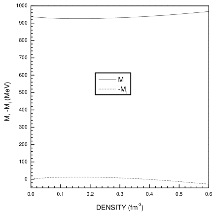
The physical meaning of the equivalent mass is that nucleons should have the equivalent mass if the system is free but with unchanged energy. It is not difficult to prove that such an equivalent mass always exists. In principle, if one obtain the energy density $\epsilon_{\text{N}}$ with some realistic models or even from QCD in the future, the equivalent mass $M$ can be obtained by solving the equation (52). For example, Fig. 3 shows the result from the Dirac-Brueckner method with Bonn-B potential Machleidt .

It should be emphasized that the equivalent mass $M$ is different from the conventional effective mass $M^{*}$ of nucleons. For example, at lower densities in Quantum Hadrondynamics (QHD) Walecka , the equivalent mass and effective mass can be expressed as

$$M^{*} = M_{\text{N}}-\frac{g_{\sigma}^{2}}{M_{\sigma}^{2}}\rho,$$ (58)

$$M = M_{\text{N}}-\frac{1}{2}\left(\frac{g_{\sigma}^{2}}{M_{\sigma}^{2}}-\frac{g_{\omega}^{2}}{M_{\omega}^{2}}\right)\rho,$$ (59)

where $M_{\sigma}=550$ MeV and $M_{\omega}=783$ MeV are, respectively, the masses for the $\sigma$ and $\omega$ mesons, and $g_{\sigma}=10.2$ and $g_{\omega}=12.55$ are the corresponding coupling constants.

It is obvious from Eqs. (58) and (59) that the conventional effective mass includes merely the contribution from scalar mesons while the equivalent mass also includes the contribution from other mesons.

Equations (58) and (59) are obtained as such. The QHD Lagrangian is

$$L = \bar{\Psi}\left[\gamma^{\mu}(i\partial_{\mu}-g_{\omega}\omega_{\mu})-(M_{N}-g_{\sigma}\sigma)\right]\Psi+\frac{1}{2}\partial_{\mu}\sigma\partial^{\mu}\sigma$$ (60)

$$-\frac{1}{2}M_{\sigma}^{2}\sigma^{2}-\frac{1}{4}F_{\mu\nu}F^{\mu\nu}+\frac{1}{2}M_{\omega}^{2}\omega_{\mu}\omega^{\mu}.$$

At the mean-field level, we have the following energy density Walecka

$$\epsilon_{\text{QHD}} = g_{N}\int^{p_{\text{f}}}_{0}\sqrt{p^{2}+{M^{*}}^{2}}\frac{d^{3}p}{(2\pi)^{3}}$$ (61)

$$+\frac{M_{\sigma}^{2}}{2g_{\sigma}^{2}}\left(M_{N}-M_{N}^{*}\right)^{2}+\frac{g_{\omega}^{2}}{2M_{\omega}^{2}}\rho^{2},$$

where the effective mass $M^{*}$ is determined by the self-consistent equation

$$M^{*}=M_{N}-\frac{g_{\sigma}^{2}}{M_{\sigma}^{2}}\frac{g_{N}}{2\pi^{2}}\int_{0}^{p_{\text{f}}}\frac{M^{*}p^{2}dp}{\sqrt{p^{2}+{M^{*}}^{2}}}$$ (62)

obtained by minimizing the energy density Eq. (61).

Taking the approximation $\sqrt{p^{2}+{M^{*}}^{2}}\approx M^{*}$ in Eq. (62) gives Eq. (58) immediately. As for Eq. (59), it should be solved from

$$\epsilon_{N}(M,\rho)=\epsilon_{\text{QHD}}.$$ (63)

Here the $\epsilon_{N}(M,\rho)$ is the right hand side (r.h.s.) of Eq. (52) and $\epsilon_{\text{QHD}}$ is the r.h.s. of Eq. (61). Taking the approximation

$$\sqrt{p^{2}+M^{2}}\approx M\ \mbox{and}\ \sqrt{p^{2}+{M^{*}}^{2}}\approx M^{*}$$ (64)

in Eq. (63), Eq. (59) is accordingly obtained.

Figure 4: The effective mass $M^{*}$, the equivalent mass $M$, and the interaction mass $M_{\text{I}}$ vary with density in QHD.

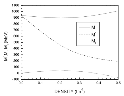
Naturally, Eqs. (58) and (59) are valid only to first order in density. For accurate relations, we have solved Eqs. (62) and (63) numerically. The results are plotted in Fig. 4.

From Fig. 3 and Fig. 4, we see clearly that $M_{\text{I}}$ is much smaller than $M_{\text{N}}$. Up to three times the normal nuclear density, $M_{\text{I}}$ is less than 6 percent of $M_{\text{N}}$. Also, when the density does not exceed the deconfinement density, $M_{\text{I}}$ must be a continuous function of density. Therefore, we ignore the second term in the bracket of Eq. (55), and get

$$\frac{\langle\bar{q}q\rangle_{\rho}}{\langle\bar{q}q\rangle_{0}}=1-\frac{\rho}{\rho^{*}}f\left(\frac{p_{\text{f}}}{M}\right).$$ (65)

Because the second term in the bracket of Eq. (56) has a factor $m_{0}/\sigma_{\text{N}}$ which is much smaller than 1, we can also ignore the corresponding term and get the same expression.

Due to the smallness of the ratio $p_{\text{f}}/M$ at lower densities, the function $f(p_{\text{f}}/M)$ approaches to unity. Accordingly, Eq. (65) becomes Eq. (38), although Eq. (65) is in principle more accurate. Naturally, if one wants to study the higher density behavior of the quark condensate in nuclear matter, the function $f(p_{\text{f}}/M)$ should be kept. Also at higher densities, the omitted interacting part $M_{\text{I}}$ should be taken into account. In the following, we try to consider it in the mean-field level.

As has been found by Malheiro et al. Malheiro97 , the quark condensate can also be linked to the trace of energy-momentum tensor of nuclear matter, i.e.

$$\frac{\langle\bar{q}q\rangle_{\rho}}{\langle\bar{q}q\rangle_{0}}=1-\frac{1}{\rho^{*}}\frac{\epsilon_{\text{N}}-3P}{M_{\text{N}}}.$$ (66)

To continue our discussion, we now adopt this equality directly in our present model. Because it is justified by Malheiro et al. Malheiro97  in the mean-field approximation of Walecka, ZM, and ZM3 models, our treatment in the following are expected to be at least valid at mean-field level. In our case, the energy density $\epsilon_{\text{N}}$ is related to the equivalent mass $M$ by Eq. (52) which, after performing the integration, gives

$$\epsilon_{\text{N}}(M,\rho)=M\rho F\left(\frac{p_{\text{f}}}{M}\right).$$ (67)

Here the function $F$ is the same as in Eq. (13).

The pressure $P$ can be obtained from Eq. (67), i.e.

$$P=M\rho G\left(\frac{p_{\text{f}}}{M}\right)+\rho^{2}\frac{\partial M}{\partial\rho}f\left(\frac{p_{\text{f}}}{M}\right),$$ (68)

where the function $f$ is given by Eq. (13), the function $G$ is defined to be

$$G(x)=\frac{1}{8}\left[x(2x^{2}-3)\sqrt{x^{2}+1}+3\mbox{arcsinh}(x)\right]/x^{3}.$$ (69)

The second term on the r.h.s. of Eq. (68) is from the density dependence of the equivalent mass. In obtaining the pressure $P$, one should be very careful. Otherwise, inconsistencies will appear in this model. For thermodynamic details, see our recent publication PengPRC62 .

Combining Eqs. (55) and (66) gives

$$\frac{\rho}{3n^{*}}f\left(\frac{p_{\text{f}}}{M}\right)\frac{\partial M}{\partial m_{0}}=\frac{1}{\rho^{*}}\frac{\epsilon_{\text{N}}-3P}{M_{\text{N}}}.$$ (70)

substituting Eqs. (67) and (68) into Eq. (70), we have

$$\frac{\rho^{*}}{3n^{*}}\frac{\partial M}{\partial m_{0}}=\frac{M}{M_{\text{N}}}\left[\frac{F(p_{\text{f}}/M)-3G(p_{\text{f}}/M)}{f(p_{\text{f}}/M)}-\frac{3\rho}{M}\frac{\partial M}{\partial\rho}\right].$$ (71)

Because of the equalities,

$$\frac{F(x)-3G(x)}{f(x)}=1\ \ \mbox{and}\ \ \frac{\rho^{*}}{3n^{*}}=\frac{m_{0}}{\sigma_{\text{N}}},$$ (72)

Eq. (71) can be cast to

$$\frac{m_{0}}{\sigma_{\text{N}}}\frac{\partial M}{\partial m_{0}}+\frac{3\rho}{M_{\text{N}}}\frac{\partial M}{\partial\rho}=\frac{M}{M_{\text{N}}}.$$ (73)

This partial differential equation is linear and of first order. To find a special solution for our purpose, let’s expand the equivalent mass $M$ in a Taylor series at zero density, i.e.

$$M(\rho,m_{0})=\sum_{i}c_{i}\rho^{i}=c_{0}+c_{1}\rho+c_{2}\rho^{2}+c_{3}\rho^{3}.$$ (74)

In principle, this expansion can have an arbitrarily large number of higher order terms in density. But, for the moment, we only consider terms up to the third order in density. We will discuss this problem at the end of this section.

Substituting Eq. (74) into Eq. (73) leads to

$$\frac{m_{0}}{\sigma_{\text{N}}}\sum_{i}{c_{i}}^{\prime}\rho^{i}+\frac{3}{M_{\text{N}}}\sum_{i}ic_{i}\rho^{i}=\frac{1}{M_{\text{N}}}\sum_{i}c_{i}\rho^{i},$$ (75)

where ${c_{i}}^{\prime}\equiv dc_{i}/dm_{0}$. Comparing the coefficients in Eq. (75), we have

$${c_{i}}^{\prime}=-\frac{\sigma_{\text{N}}}{m_{0}}\frac{3i-1}{M_{\text{N}}}c_{i},$$ (76)

or explicitly,

$${c_{0}}^{\prime} = \frac{\sigma_{\text{N}}}{m_{0}}\frac{c_{0}}{M_{\text{N}}},$$ (77)

$${c_{1}}^{\prime} = -2\frac{\sigma_{\text{N}}}{m_{0}}\frac{c_{1}}{M_{\text{N}}},$$ (78)

$${c_{2}}^{\prime} = -5\frac{\sigma_{\text{N}}}{m_{0}}\frac{c_{2}}{M_{\text{N}}},$$ (79)

$${c_{3}}^{\prime} = -8\frac{\sigma_{\text{N}}}{m_{0}}\frac{c_{3}}{M_{\text{N}}}.$$ (80)

From Eqs. (51) and (74), we can easily get $c_{0}=M_{\text{N}}$. In this case, Eq. (77) becomes ${c_{0}}^{\prime}=\sigma_{\text{N}}/m_{0}$, which is consistent with Eq. (57).

It should be pointed out that the coefficients $c_{i}$ in the Taylor expansion (74) are $m_{0}$-dependent. In fact, we can integrate Eq. (76) and get

$$c_{i}=c_{i}(7.5)\left[\exp\left({-\int_{7.5}^{m_{0}}\frac{\sigma_{\text{N}}}{M_{\text{N}}}\frac{dm_{0}}{m_{0}}}\right)\right]^{3i-1},$$ (81)

where $c_{i}(7.5)$ is the value for $c_{i}$ at $m_{0}=7.5$ MeV which is the value we take for the current mass of $u$ and $d$ quarks.

Now let’s substitute Eq. (74) into Eq. (55) or (56) and get

$$\frac{\langle\bar{q}q\rangle_{\rho}}{\langle\bar{q}q\rangle_{0}}=1-\frac{\rho}{\rho^{*}}f\left(\frac{p_{\text{f}}}{M}\right)\left[1+\frac{m_{0}}{\sigma_{\text{N}}}\sum_{i=1}^{3}{c_{i}}^{\prime}\rho^{i}\right].$$ (82)

On applying Eq. (76), we finally have

$$\frac{\langle\bar{q}q\rangle_{\rho}}{\langle\bar{q}q\rangle_{0}}=1-\frac{\rho}{\rho^{*}}f\left(\frac{p_{\text{f}}}{M}\right)\left[1-\frac{1}{M_{\text{N}}}\sum_{i=1}^{3}(3i-1)c_{i}\rho^{i}\right].$$ (83)

For figure-plotting convenience, let’s change the coefficients $c_{i}$ (i=1,2,3) to $a_{i}$ by defining

$$a_{i}=\frac{{\rho_{0}}^{i}}{M_{\text{N}}}c_{i}\ \mbox{or}\ c_{i}=\frac{M_{\text{N}}}{{\rho_{0}}^{i}}a_{i}.$$ (84)

Accordingly, Eqs. (74) and (83) become, respectively,

$$\frac{M}{M_{\text{N}}} = 1+a_{1}\frac{\rho}{\rho_{0}}+a_{2}\left(\frac{\rho}{\rho_{0}}\right)^{2}+a_{3}\left(\frac{\rho}{\rho_{0}}\right)^{3},$$ (85)

$$\frac{\langle\bar{q}q\rangle_{\rho}}{\langle\bar{q}q\rangle_{0}} = 1-\frac{\rho}{\rho^{*}}f\left(\frac{p_{\text{f}}}{M}\right)\left[1-\sum_{i=1}^{3}(3i-1)a_{i}\left(\frac{\rho}{\rho_{0}}\right)^{i}\right].$$ (86)

To obtain the values of the coefficients $a_{1},a_{2}$, and $a_{3}$, we can use the following known experimental properties of nuclear matter

$$\left.\frac{\epsilon_{\text{N}}(M,\rho)}{\rho}\right|_{\rho=\rho_{0}}=M_{\text{N}}+E_{\text{b}},$$ (87)

$$\frac{d}{d\rho}\left.\left[\frac{\epsilon_{\text{N}}(M,\rho)}{\rho}\right]\right|_{\rho=\rho_{0}}=0,$$ (88)

$$9\rho_{0}^{2}\frac{d^{2}}{d\rho^{2}}\left.\left[\frac{\epsilon_{\text{N}}(M,\rho)}{\rho}\right]\right|_{\rho=\rho_{0}}=K.$$ (89)

Here $\rho_{0}=0.17$ fm^-3 is the normal nuclear saturation density, $E_{\text{b}}=-16$ MeV is the nuclear binding energy. As for the incompressibility $K$, it is not so definite, maybe ranging from 150 to 350 MeV. The expression $\epsilon_{\text{N}}(M,\rho)/\rho=MF(p_{\text{f}}/M)$ is the energy per nucleon. For a given $K$, we can solve Eqs. (87-89) and get the values for $M^{(i)}$ ($i$=0,1,2):

$$M^{(0)} \equiv \left.M\right|_{\rho=\rho_{0}},$$ (90)

$$M^{(1)} \equiv \left.\frac{\partial M}{\partial\rho}\right|_{\rho=\rho_{0}},$$ (91)

$$M^{(2)} \equiv \left.\frac{\partial^{2}M}{\partial\rho^{2}}\right|_{\rho=\rho_{0}}.$$ (92)

Substituting the expansion (85) into the right hand side of Eqs. (90-92) and then solving for $a_{1},a_{2}$, and $a_{3}$, we have

$$a_{1} = \frac{-1}{M_{\text{N}}}\left[3(M_{\text{N}}-M^{(0)})+2M^{(1)}\rho_{0}-\frac{1}{2}M^{(2)}{\rho_{0}}^{2}\right],$$ (93)

$$a_{2} = \frac{1}{M_{\text{N}}}\left[3(M_{\text{N}}-M^{(0)})+3M^{(1)}\rho_{0}-M^{(2)}{\rho_{0}}^{2}\right],$$ (94)

$$a_{3} = \frac{-1}{M_{\text{N}}}\left[M_{\text{N}}-M^{(0)}+M^{(1)}\rho_{0}-\frac{1}{2}M^{(2)}{\rho_{0}}^{2}\right].$$ (95)

The quark condensate can then be calculated by Eq. (86).

Figure 5: The coefficients $a_{1}$, $a_{2}$, and $a_{3}$ vary with the incompressibility $K$. The dotted line gives the corresponding critical density $\rho_{\text{c}}$ at which the quark condensate becomes zero. The full line is the deconfinement density $\rho_{\text{d}}$ after which the deconfinement phase transition is expected to occur.

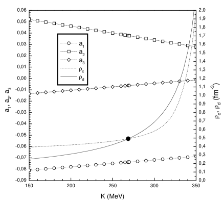
In Fig. 5, we give, on the left axe, the coefficients $a_{1},a_{2}$, and $a_{3}$ as a function of $K$. Another two lines on the right axe are to be explained a little later.

Figure 6: Equation of state of nuclear matter for different incompressibilities in the present approach. The open circle corresponds to the saturation. After the solid circle, nuclear matter will automatically contract, and the deconfinement phase is expected to occur.

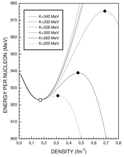
Fig. 6 shows the equation of state of nuclear matter for typical incompressibilities. The open circle corresponds to the saturation which is a mechanically stable point, so every line passes it by. The points marked with a solid circle are also in mechanical equilibrium, but they are not stable. When the density is between the open and solid circle, the pressure is positive. However, when the density exceeds the full circle, the pressure is drastically negative, so the system will automatically contract and the deconfinement phase is expected to appear. We therefore use $\rho_{\text{d}}$ to remember this density and plot it in Fig. 5 with a solid line on the right axe. We can also see that the incompressibility $K$ should be no less than 265 MeV because nuclear matter will be less bounded than 16 MeV on the right side when $K<265$, i.e. the difference of the energy corresponding to the solid and open circles is smaller than 16 MeV if $K$ is less than 265 MeV.

Figure 7: The Quark condensate in nuclear matter to its vacuum value in the present model. When the incompressibility $K$ is in the range 265–326 MeV, the condensate decreases monotonously with increasing density. When $K$ is bigger than 326 MeV, there appears a hill where the chiral symmetry breaking might be enhanced. In both case, the critical density for the condensate becomes zero is higher than the linear extrapolation.

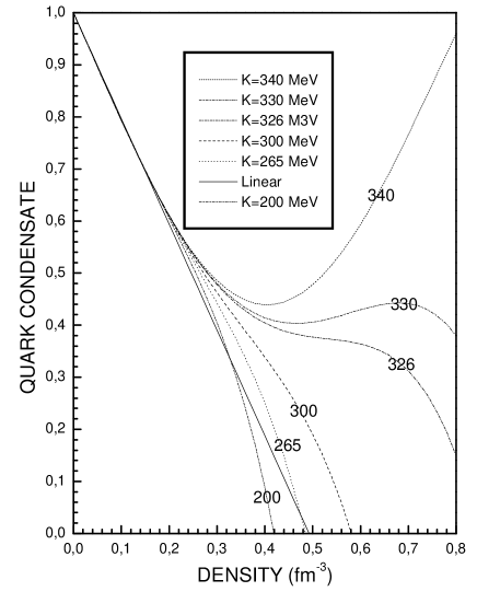
The quark condensate is given in Fig. 7 for typical values of $K$. For $K>265$, the critical density $\rho_{\text{c}}$ where the quark condensate becomes zero is generally bigger than that obtained by extrapolating the model-independent result of Eq. (38) (indicated with the word ’Linear’ in the figure legend). The variation of the critical density with the incompressibility is shown in Fig. 5 with a dotted line on the right axe. A noticeable feature is that, for $K>326$, there appears a hill where the chiral symmetry breaking might be enhanced.

As mentioned before, the Taylor expansion Eq. (74) can have infinitely large number of terms in density. However, it has been obviously shown in Fig. 5 that

$$|a_{1}|>|a_{2}|>|a_{3}|.$$ (96)

This is an indication that the higher the term’s order is, the less important its contribution. This is why we have only taken to the third order in the expansion Eq. (74). However, it is very easy to extend to even higher orders. For this purpose, we should first express the equivalent mass as

$$M(\rho,m_{0})=\sum_{i=0}^{J}c_{i}\rho^{i},$$ (97)

where $J$ is an integer. It’s value depends on to which order we would like to expand. In the case we have just treated, $J=3$.

The initial values for

$$M^{(i)}\equiv\left.\frac{\partial^{i}M}{\partial\rho^{i}}\right|_{\rho=\rho_{0}}\ \ \ \ (i=0,\cdots,J-1)$$ (98)

are solved from

$$(3\rho_{0})^{i}\frac{d^{i}}{d\rho^{i}}\left.\left[\frac{\epsilon_{\text{N}}(M,\rho)}{\rho}\right]\right|_{\rho=rho_{0}}=K_{i},\ \ \ (i=0\cdots J-1),$$ (99)

where $K_{0}=M_{\text{N}}+E_{\text{b}},K_{1}=0,K_{2}=K$. If $J>3$, we should also know the information on $K_{3},K_{4}$ et al.. The coefficients $c_{i}$ $(i=1\dots J)$ are obtained by solving

$$\sum_{i=k}^{J}\frac{i!}{(i-k)!}c_{i}{\rho_{0}}^{i}=M^{(k)},\ \ \ (k=0\cdots J-1).$$ (100)

And the quark condensate is

$$\frac{\langle\bar{q}q\rangle_{\rho}}{\langle\bar{q}q\rangle_{0}}=1-\frac{\rho}{\rho^{*}}f\left(\frac{p_{\text{f}}}{M}\right)\left[1-\sum_{i=1}^{J}(3i-1)a_{i}\left(\frac{\rho}{\rho^{0}}\right)^{i}\right].$$ (101)

Here the relation between $a_{i}$ and $c_{i}$ is still given by Eq. (84).

IV Summary

We have presented a new formalism for the calculation of the in-medium chiral condensates. The key point of this scheme is to obtain an equivalent mass by solving a differential equation. The main advantage is that one does not need to make further assumptions on the derivatives of model parameters with respect to the quark current mass.

As an application of this method, we have successfully reproduced the normally accepted model-independent result in nuclear matter. We also showed that there is a similar expression for the chiral condensate in quark matter. It is found that the pion-nucleon sigma term is six times the average light quark current mass if the two decreasing speed is equal.

For quark matter at higher densities, we adopted a QCD-like interaction to solve our differential equation, which shows that the condensate decreases linearly at lower densities. However, the decreasing speed is slowed at higher densities, compared with the linear extrapolation. For some values of the parameters, it can finally vanish, while for other values it may saturate and even increase.

We have also shown that the incompressibility $K$ should not be less than 265 MeV to give the correct nuclear binding energy in this model. When $K$ is in the range of 265 to 326 MeV, the quark condensate monotonously decreases with increasing density. However, the critical density where the condensate vanishes is, generally, higher than that obtained by linear extrapolation. When $K$ is greater than 326 MeV, a hill for the condensate as function of density will appear, enhancing the chiral symmetry breaking, vanishing then for even higher densities.

References

• (1) G.E. Brown and M. Rho, Phys. Rep. 363, 85 (2002).
• (2) T. Hatsuda, T. Kunihiro, and H. Shimizu, Phys. Rev. Lett. 82, 2840 (1999).
• (3) T.D. Cohen and L.Ya. Glozman, Int. J. Mod. Phys. A 17, 1327 (2002).
• (4) M. Harada and K. Yamawaki, Phys. Rev. Lett. 86, 757 (2001).
• (5) R. Rapp, R. Machleidt, J.W. Durso, and G.E. Brown, Phys. Rev. Lett. 82, 1827 (1999).
• (6) A.B. Santra and U. Lombardo, Phys. Rev. C 62, 018202 (2000).
• (7) M.C. Birse, Phys. Rev. C 53, R2048 (1996).
• (8) I.P. Cavalcante and J. SΓ‘ Borges, Phys. Rev. D 63, 114022 (2001).
• (9) G. Colangelo, J. Gasser, and H. Leutwyler, Phys. Rev. Lett. 86, 5008 (2001).
• (10) J-L. Ballot, M. Ericson, and M.R. Robilotta, Phys. Rev. C 61, 055202 (2000).
• (11) E.G. Drukarev, M.G. Ryskin, V.A. Sadovnikova, Prog. Part. Nucl. Phys. 47, 73 (2001); Eur. Phys. J. A 4, 171 (1999); Z. Phys. A 353, 455 (1996).
• (12) T.D. Cohen, R.J. Furnstahl, and D.K. Griegel, Phys. Rev. C 45, 1881 (1992); Phys. Rev. Lett. 67, 961 (1991).
• (13) G. Chanfray and M. Ericson, Nucl. Phys. A 556, 427 (1993); J. Delorme, G. Chanfray, and M. Ericson, Nucl. Phys. A 603, 239 (1996); G. Chanfray, M. Ericson, and J. Wambach, Phys. Lett. B 388, 673 (1996).
• (14) M. Lutz, S. Klimt, and W. Weise, Nucl. Phys. A 542, 52 (1992); M. Lutz, B. Friman, and Ch. Appel, Phys. Lett. B 474, 7 (2000).
• (15) H. Guo, S. Yang, and Y.X. Liu, Sci. Chin. Ser. A 44, 1042 (2001); Commun. Theor. Phys. 34, 471 (2000); J. Phys. G 25, 1701 (1999).
• (16) M. Malheiro, M. Dey, A. Delfino, and J. Dey, Phys. Rev. C55, 521 (1997).
• (17) Z.S. Wang, Z.Y. Ma, and Y.Z. Zhuo, Z. Phys. A 358, 451 (1997).
• (18) T. Mitsumori, N. Noda, H. Kouno, A. Hasegawa, and M. Nakano, Phys. Rev. C 55, 1577 (1997).
• (19) L. Li, P.Z. Ning, W.Q. Li, Chin. Phys. Lett. 13, 813 (1996).
• (20) R. Brockmann and W. Weise, Phys. Lett. B 367, 40 (1996).
• (21) H. Fojii and Y. Tsue, Phys. Lett. B 357, 199 (1995).
• (22) G.Q. Li and C.M. Ko, Phys. Lett. B 338, 118 (1994).
• (23) V. Bernard, Ulf-G. Meissner, and I. Zahed, Phys. Rev. D 36, 819 (1987); V. Bernard and Ulf-G. Meissner, Nucl. Phys. 489, 647 (1988).
• (24) M. Jaminon, R.M. Galain, G. Ripka, and P. Stassart, Nucl. Phys. A 537, 418 (1992).
• (25) M.C. Birse, J. Phys. G 20, 1537 (1994); Acta Phys. Polon. B 29, 2357 (1998).
• (26) E. Witten, Phys. Rev. D 30, 272 (1984).
• (27) E. Farhi and R.L. Jaffe, Phys. Rev. D 30, 2379 (1984); M.S. Berger and R.L. Jaffe, Phys. Rev. C 35, 213 (1987); E.P. Gilson and R.L. Jaffe, Phys. Rev. Lett. 71, 332 (1993).
• (28) G.X. Peng, P.Z. Ning, and H.Q. Chiang, Phys. Rev. C 56, 491 (1997).
• (29) S. Chakrabarty, S. Raha, and B. Sinha, Phys. Lett. B 229, 112 (1989); S. Chakrabarty, Phys. Rev. D 43, 627 (1991); D 48, 93 (1993); D 54, 1306 (1996).
• (30) O.G. Benvenuto and G. Lugones, Phys. Rev. D 51, 1989 (1995); G. Lugones and O.G. Benvenuto, ibid. 52, 1276 (1995).
• (31) Y. Zhang and R.K. Su, Phys. Rev. C 65, 035202 (2002); Y. Zhang, R.K. Su, and P. Wang, Europhys. Lett. 56, 361 (2001); P. Wang, Phys. Rev. C 62, 015204 (2000).
• (32) G.X. Peng, H.C. Chiang, P.Z. Ning, and B.S. Zou, Phys. Rev. C 59, 3452 (1999).
• (33) G.X. Peng, H.C. Chiang, J.J. Yang, L. Li, and B. Liu, Phys. Rev. C 61, 015201 (2000).
• (34) G.X. Peng, H.C. Chiang, B.S. Zou, P.Z. Ning, and S.J. Luo, Phys. Rev. C 62, 025801 (2000).
• (35) M. Gell-Mann, R. Oakes, and B. Renner, Phys. Rev. 175, 2195 (1968).
• (36) G.X. Peng, U. Lombardo, M. Loewe, and H.C. Chiang, Phys. Lett. B 548, 189 (2002).
• (37) J. Gasser, H. Leutwyler, and M. Sainio, Phys. Lett. B 253, 252 (1991).
• (38) T.E.O. Ericson, Phys. Lett. B 195, 116 (1987).
• (39) P.M. Gensini, Nuovo Cimento 60A, 221 (1980).
• (40) M.K. Banerjee and J.B. Cammarata, Phys. Rev. D 16, 1334 (1977).
• (41) M. Sainio, $\pi$N Newsletter 10, 13 (1995).
• (42) W.R. Gibbs, Li Ai, and W.B. Kaufmann, Phys. Rev. C 57, 784 (1998).
• (43) J. Gasser and H. Leutwyler, Phys. Rep. 87, 77 (1982).
• (44) E. Eichten, K. Gottfried, T. Kinoshita, J. Kogut, K.D. Lane, and T.M. Yan, Phys. Rev. Lett. 34, 369 (1975).
• (45) J.L. Richardson, Phys. Lett. B 82, 272 (1979).
• (46) W. Fischler, Nucl. Phys. B 129, 157 (1977).
• (47) A. Billiore, Phys. Lett. B 92, 343 (1980).
• (48) C. Quigg and J. Rosner, Phys. Lett. B 71, 153 (1977).
• (49) A. Martin, Phys. Lett. B 93, 338 (1980).
• (50) C. Quigg and J.L. Rosner, Phys. Rev. D 23, 2625 (1981).
• (51) Y.I. Kogan and V.M. Belyaev, Phys. Lett. B 136, 273 (1984); K.D. Born, E. Laermann, N. Pirch, T.F. Walsh, and P.M. Zerwas, Phys. Rev. D 40, 1653 (1989).
• (52) N. Isgur and J. Paton, Phys. Lett. B 124, 247 (1983); Phys. Rev. D 31, 2910 (1985).
• (53) K. Igi and S. Ono, Phys. Rev. D 33, 3349 (1986).
• (54) S. Veseli and M. Olsson, Phys. Lett. B 383, 109 (1996).
• (55) J. Gasser, Ann. Phys. 136, 62 (1981).
• (56) M. Musakhanov, Nucl. Phys. A 699, 340 (2002).
• (57) R. Machleidt, in Computational nuclear physics 2 β€” nuclear reaction, eds. K. Langank, J.A. Maruhn, S.E. Koonin, (Springer-Verlag, New York, 1993), Chap.1, p.1.
• (58) B.D. Serot and J.D. Walecka, Int. J. Mod. Phys. E 6, 515 (1997); Adv. Nucl. Phys. 16, 1 (1986).