http://xxx.lanl.gov/abs/hep-ph/0304220

Abstract

We present approximate non-perturbative solutions for the propagators as well as the running coupling of QCD. We solve a coupled system of renormalised, truncated Dyson–Schwinger equations for the ghost, gluon and quark propagators in flat Euclidean space-time. We employ ansätze for the dressed vertices such that the running coupling and the quark mass function are independent of the renormalisation point. At large momenta we obtain the correct one-loop anomalous dimensions for all propagators. Our solutions are in good agreement with the results of recent lattice calculations.

In the Yang-Mills sector of Landau gauge QCD we find a weakly vanishing gluon propagator in the infrared and a ghost propagator more singular than a simple pole. This is in accordance with Zwanziger’s horizon condition and the Kugo-Ojima confinement criterion. The running coupling possesses an infrared fixed point at $\alpha(0)=8.92/N_{c}$. To investigate the influence of boundary conditions on the propagators we solved the ghost and gluon DSEs also on a four-torus. Our results show typical finite volume effects but are still close to the continuum solutions for sufficiently large volumes.

In general ghost-antighost symmetric gauges we study the infrared behaviour of the ghost and gluon propagators. No power-like solutions exist when replacing all dressed verticed with bare ones. The results of the Landau gauge limit are recovered from a different direction in gauge parameter space.

For the quark propagator we find dynamically generated quark masses that agree well with phenomenological values and corresponding results from lattice calculations. The effects of unquenching the system are found to be small. In particular the infrared behaviour of the ghost and gluon dressing functions found in pure Yang-Mills theory is almost unchanged as long as the number of light flavors is smaller than four.

Keywords: Confinement, dynamical chiral symmetry breaking, running coupling, gluon propagator, quark propagator, Dyson-Schwinger equations, infrared behaviour

Note added to the eprint-version

This PhD-thesis has been submitted to the University of Tübingen in November 2002 and has been accepted in March 2003. Chapters 3 and 5 of this thesis are based on refs.[83,84] (hep-ph/0202195, hep-ph/0202202), however some material has been reordered and more detailed explanations have been added. The contents of chapter 6 are published in ref.[140] (hep-th/0301094). Chapter 4 represents the research status of November 2002. The contents of this chapter together with recent results on ghost-antighost symmetric gauges can be found in ref.[109] (hep-th/0304134).

Non-perturbative Propagators, Running

Coupling and Dynamical Mass Generation

in Ghost-Antighost Symmetric Gauges in

QCD

Dissertation
zur Erlangung des Grades eines

Doktors der Naturwissenschaften

der Fakultät für Mathematik und Physik

der Eberhard-Karls-Universität zu Tübingen

vorgelegt von

Christian S. Fischer
aus Illertissen

2003

Chapter 1 Introduction

Quantum Chromo Dynamics (QCD) is the quantum field theory which describes the strong interaction of the fundamental building blocks of matter, the quarks and gluons [1, 2, 3, 4, 5, 6]. In contrast to Abelian gauge theories like Quantum Electro Dynamics (QED), the non-Abelian nature of the gauge symmetry of QCD not only induces interactions between quarks and gluons but also among gluons themselves. This last effect is expected to generate the phenomenon of confinement, i.e. the permanent inclusion of all colour charges in colour neutral objects, the hadrons.

’Quantum chromo dynamics is a Lagrangian field theory in search of a solution.’ This statement, quoted from the classical review of Marciano and Pagels on QCD [7], has not lost its relevance since it has been written down in 1977. Although in the meantime a lot of progress has been made it is still not clear how the plethora of observed bound state objects, the hadrons, can arise from the fundamental quark and gluon fields of QCD. In the last thirty years a lot of different strategies have been employed to explore both the large and small momentum properties of hadrons. The physical phenomena encountered at large momentum transfers are very well described by perturbation theory. Asymptotic freedom means that the interaction strength of QCD tends to zero at small distances. High energy probes therefore picture hadrons as quark and gluon lumps with definite quantum numbers described by so called structure functions. This picture, however, starts to break down at energies around 1-2 GeV and is surely inadequate at length scales corresponding to the size of the nucleon. At such scales the strong interaction is strong enough to invalidate perturbation theory and one has to employ completely different methods to deal with what is called Strong QCD.

There are two phenomena of QCD which are important for this work: the mechanism of confinement and that of dynamical chiral symmetry breaking, i.e. the generation of quark masses via interactions. Neither of these phenomena can be accounted for in perturbation theory, thus they are genuine effects of Strong QCD. Interestingly, both phenomena appear to be connected. From finite temperature studies of QCD we infer that both effects seem to disappear at roughly the same temperature but the reasons for this are yet unclear [8].

The framework chosen in this work to investigate the small momentum regime of QCD are the Dyson-Schwinger equations of motion for correlation functions of the fields. Certainly a great step forward in understanding QCD would be the detailed knowledge of the basic correlation functions, the propagators. Information on certain confinement mechanisms is encoded in these two-point functions. Furthermore the mechanism of dynamical chiral symmetry breaking can be studied directly in the Dyson-Schwinger equation for the quark propagator, which is the gap equation of QCD. Besides being related to the fundamental issues of QCD, the quark and gluon propagators are vital ingredients for phenomenological models describing low and medium energy hadron physics. Bound state calculations based on the Bethe-Salpeter equations for mesons or on the Faddeev equations for baryons (for reviews see [9, 10]) might one day be capable to bridge the gap between the fundamental theory, QCD, and phenomenology.

Throughout this work we will compare the results obtained from Dyson-Schwinger equations with those of lattice Monte Carlo simulations (see e.g. [11]). Combining the strengths and weaknesses of both approaches allows one to make quite definite statements for the propagators in a large momentum range. Lattice Monte Carlo simulations include all non-perturbative physics of Yang-Mills theories and are therefore the only ab initio calculation method available so far. However, the simulations suffer from limitations at small momenta due to finite volume effects. One has to rely on extrapolation methods to obtain the infinite volume limit. Furthermore calculations including quarks are subtle on the lattice, as it is very difficult to implement fermions with small bare masses. On the other hand Dyson-Schwinger equations can be solved analytically in the infrared and are the proper tool to assess the effects of dynamical quarks. However, in order to obtain a closed system of equations one has to employ ansätze for higher correlations functions. The quality of these truncations can be ascertained by comparison with lattice results.

We will recall in the next chapter some basic aspects of Strong QCD. Based on the symmetries of the (generalised) QCD Lagrangian certain aspects of dynamical chiral symmetry breaking as well as confinement are reviewed. In particular we will recall how information on the so called Kugo-Ojima confinement mechanism, the notion of positivity and Zwanziger’s horizon condition are encoded in the propagators of QCD. From the generalised QCD Lagrangian of Baulieu and Thierry-Mieg [12] we will derive a modified Dyson-Schwinger equation for the ghost propagator, which together with the corresponding equations for the gluon and quark propagators are the basic tools of our investigation.

The third chapter is devoted to Landau gauge, where a novel truncation scheme is introduced that allows to solve the coupled ghost and gluon Dyson-Schwinger equations of pure Yang-Mills theory. Contrary to earlier attempts this is done without any angular approximations in the loop integrals of the equations. Besides the numerical solutions for general momenta we obtain analytical results for the ultraviolet and infrared region of momentum. We are thus able to show that the anomalous dimensions of one-loop perturbation theory are reproduced by our solutions for the full ghost and gluon propagators. For small momenta the ghost and gluon dressing functions follow power laws, which are in accordance with the Kugo-Ojima confinement criterion as well as Zwanziger’s horizon condition. We are able to show that only one out of two infrared solutions already found in earlier investigations is connected to the numerical solutions for general momenta. The resulting running coupling possesses an infrared fixed point. Our results for the propagators are in nice agreement to recently obtained lattice calculations.

Landau gauge is a special gauge in the sense that it allows for surprisingly simple vertex ansätze in the truncation of the Dyson-Schwinger equations. In chapter four we will explore whether a truncation employing bare vertices can be extended to general gauges. We solve the corresponding Dyson-Schwinger equations analytically in the infrared employing power laws for the dressing functions. The main results of Landau gauge, an infrared vanishing gluon propagator and an infrared diverging ghost turn out to be persistent for the class of linear covariant gauges. However, no power law solutions for general ghost-antighost symmetric gauges can be found. Numerical solutions for the limit of Landau gauge from different directions in gauge parameter space turn out to be stable.

In chapter five we change the base manifold and investigate the Dyson-Schwinger equations of Landau gauge Yang-Mills theory on a four-torus. There are three ideas motivating such a change. The first idea stems from the observation that torus calculations share the finite volume problem with lattice Monte Carlo simulations. However, as the continuum limit is known in the framework of Dyson-Schwinger equations, one is able to judge extrapolation methods on a torus. Our solution for the gluon propagator on a torus resembles closely the one found in the continuum whereas the ghost dressing function deviates in the very infrared. The second idea is a technical one. Although the treatment is inverted in this work, we first have been able to obtain results without angular approximations on the torus and only subsequently in the continuum. This is due to the torus acting as an effective regulator in the infrared. The third idea, which remains for future work, is to include topological obstructions like twisted boundary conditions in Dyson-Schwinger equations on a torus.

The last chapter of this work focuses on the quark propagator. We present solutions for the quenched system of quark Dyson-Schwinger equations using the results of chapter three as input, and compare to lattice calculations. We then go one step further and solve the unquenched coupled system of equations for the ghost, gluon and quark propagators of QCD. This is done without any angular approximations. Our results again reproduce the anomalous dimensions of one-loop perturbation theory in the ultraviolet. The effects of unquenching the system, i.e. including the quark loop in the gluon equation, is found to be small if the number of light flavours is small, $N_{f}^{light}<4$. In particular the infrared behaviour of the ghost and gluon dressing functions remain unchanged. The quark masses generated by dynamical chiral symmetry breaking are found to be close to phenomenological values.

Chapter 2 Aspects of Strong QCD

2.1 The generating functional of QCD

Working in Euclidean space-time the generating functional of the quantum field theory of quarks and gluons is given by

$$Z[J,\eta,\bar{\eta}] = \int{\cal D}[A\bar{\Psi}\Psi]$$

$$\exp\left\{-\int d^{4}x\left(\bar{\Psi}\left(-D\hskip-6.99997pt/+m\right)\Psi+\frac{1}{4}F_{\mu\nu}^{2}\right)+\int d^{4}x\left(A^{a}_{\mu}J^{a}_{\mu}+\bar{\eta}\Psi+\bar{\Psi}\eta\right)\right\},$$

where we have introduced the Grassmann valued sources $\bar{\eta}$ and $\eta$ for the quark fields $\Psi$ and $\bar{\Psi}$ and the source $J^{a}_{\mu}$ for the gauge field $A^{a}_{\mu}$. Furthermore we used the abbreviation $D\hskip-6.99997pt/=\gamma_{\mu}D_{\mu}$ with Euclidean $\gamma$-matrices and the covariant derivative $D_{\mu}$ given in eq. (2.4). The quark fields are spin-1/2 fermions which transform according to a fundamental representation of the gauge group $SU(N_{c})$. The central focus of this work is QCD, i.e. the gauge group $SU(3)$. However in the course of our investigations we will run across some results, that are valid for general gauge group $SU(N_{c})$. Some comparisons with lattice calculations will be done for $SU(2)$.

The non-Abelian gluon fields, $A^{a}_{\mu}$, transform according to the adjoint representation of the gauge group. The corresponding field strength tensor and the covariant derivative in the adjoint representation are given by

$$F_{\mu\nu}^{a} = \partial_{\mu}A_{\nu}^{a}-\partial_{\nu}A_{\mu}^{a}-gf^{abc}A_{\mu}^{b}A_{\nu}^{c}\;,$$ (2.2)

$$D_{\mu}^{ab} = \partial_{\mu}\delta^{ab}+gf^{abc}A_{\mu}^{c}.$$ (2.3)

Here $g$ is the (unrenormalised) coupling constant of the theory and $f^{abc}$ are the structure constants of the gauge group. With the help of the generators $t^{a}$ of $SU(N_{c})$ we can rewrite the covariant derivative in the fundamental representation

$$D_{\mu}=\partial_{\mu}+igA_{\mu}\;,$$ (2.4)

with $A_{\mu}=A_{\mu}^{a}t^{a}$ and $[t^{a},t^{b}]=if^{abc}t^{c}$. The Lagrangian ${\cal{L}}=\bar{\Psi}\left(-D\hskip-6.99997pt/+m\right)\Psi+\frac{1}{4}F_{\mu\nu}^{2}$ of our theory is invariant under local gauge transformations.

One of the most intricate tasks in the quantisation of a field theory is the separation into physical and non-physical degrees of freedom, which is a prerequisite for the definition of the physical state space of the theory. The integration over all possible gauge field configurations $A$ in the generating functional (LABEL:genfunc) includes the ones that are gauge equivalent. Therefore the integration generates an infinite constant, the volume of the gauge group ${\cal G}$, which has to be absorbed in the normalisation. More important, the gauge freedom implies that the quadratic part of the gauge field Lagrangian has zero eigenvalues and therefore cannot be inverted. This prevents the definition of a perturbative gauge field propagator [13].

In order to single out one representative configuration from each gauge orbit

$$[A^{U}]:=\left\{A^{U}=UAU^{\dagger}+UdU^{\dagger}:U(x)\in SU(N_{c})\right\}$$ (2.5)

one has to impose the gauge fixing condition $f^{a}(A)=0$ on the generating functional. This is conveniently done by inserting the identity

$$1=\Delta[A]\int{\cal D}g\>\delta(f^{a}(A))$$ (2.6)

into the generating functional (LABEL:genfunc) and absorbing the group integration $\int{\cal D}g$ in a suitable normalisation [14]. We will discuss problems with this gauge fixing prescription in more detail in subsection 2.3.3.

In linear covariant gauges the Faddeev-Popov determinant $\Delta[A]$ reads explicitly

$$\Delta[A]=\mbox{Det}\left(-\partial_{\mu}D_{\mu}^{ab}\right)$$ (2.7)

and can be written as a functional integral over two new Grassmann valued fields $c$ and $\bar{c}$. Furthermore the gauge fixing condition $f^{a}(A)=\partial_{\mu}A^{\mu}-i\lambda B^{a}=0$ employing the auxiliary field $B$ can be represented by a Gaussian integral centred around $i\lambda B^{a}=0$ (see e.g. [5] for details). We then have

$$\Delta[A]\delta(f^{a}(A)) = \int{\cal D}[\bar{c},c,B]\exp\left\{-\int d^{4}x\left(-i\partial_{\mu}\bar{c}D_{\mu}c+iB^{a}\partial_{\mu}A^{a}_{\mu}+\frac{\lambda}{2}B^{a}B^{a}\right)\right\}\hskip 11.38109pt$$ (2.8)

$$= \int{\cal D}[\bar{c},c]\exp\left\{-\int d^{4}x\left(-i\partial_{\mu}\bar{c}D_{\mu}c-\frac{(\partial_{\mu}A_{\mu}^{a})^{2}}{2\lambda}\right)\right\}.$$

Introducing the sources $\sigma$ and $\bar{\sigma}$ for the antighost and ghost field respectively we arrive at the gauge fixed generating functional

$$Z[J,\sigma,\bar{\sigma},\eta,\bar{\eta}] = \int{\cal D}[A\bar{\Psi}\Psi c\bar{c}]$$ (2.9)

$$\exp\left\{-\int d^{4}x{\cal L}_{eff}+\int d^{4}x\left(A^{a}_{\mu}J^{a}_{\mu}+\bar{\eta}\Psi+\bar{\Psi}\eta+\bar{\sigma}c+\bar{c}\sigma\right)\right\},\hskip 11.38109pt$$

with the effective (unrenormalised) Lagrangian

$${\cal{L}}_{eff}={\cal{L}}_{M}+{\cal{L}}_{A}+{\cal{L}}_{GF}=\bar{\Psi}\left(-D\hskip-6.99997pt/+m\right)\Psi+\frac{1}{4}F_{\mu\nu}^{2}+\frac{\left(\partial_{\mu}A_{\mu}\right)^{2}}{2\lambda}-i\partial_{\mu}\bar{c}D_{\mu}c.$$ (2.10)

Note that a factor of $i$ appears in front of the ghost terms as we have used real ghost and antighost fields. We will see the importance of this choice in section 2.3.

In effect we have modified the Lagrangian of our theory with a term containing the (unphysical) ghost and antighost fields $c$ and $\bar{c}$ which transform according to the adjoint representation of the gauge group and the gauge fixing part which may or may not be written with the help of the Nakanishi-Lautrup auxiliary field $B^{a}$.

Apart from the convention of real ghost fields the Lagrangian (2.10) is the usual one employed in perturbation theory. It has some important properties:

• it is of dimension 4,

• it is Lorenz invariant and globally gauge invariant,

• it is BRS and anti-BRS invariant,

• and hermitian.

The number of dimensions and Lorenz invariance are certainly dictated by experiment. The further symmetries, global gauge invariance and BRS symmetry, are discussed in section 2.2. Hermiticity is necessary to define the physical S-matrix of the theory. We will say a little more about this issue in subsection 2.3.1.

The Lagrangian (2.10) arises from a specific gauge fixing procedure, the Faddeev-Popov method. This, however, is not the only gauge fixing procedure that has been employed so far. Indeed, as will be discussed in more detail in subsection 2.3.3, the Faddeev-Popov method is not capable to fix the gauge completely. Although it is currently not known to what extend this poses a problem for strong QCD, it is desirable to develop alternatives which do not suffer from such a deficiency. Examples for different gauge fixing procedures are topological gauge fixing [15, 16], where the aim is to represent the partition function of QCD by a topological invariant, or stochastic gauge fixing [17, 18], which employs a Fokker-Planck equation for the probability distribution in gauge field space.

On the other hand, one could reverse arguments and claim the properties (i)-(iv) to be crucial for the quantum field theory of strong interaction. Without bothering about the details of the gauge fixing procedure one could then search for the most general Lagrangian satisfying (i)-(iv). This view has been adopted in [12, 19]. It has been shown that, omitting topological terms, the most general polynomial in the fields $A_{\mu}$, $c$, $\bar{c}$, $\Psi$ and $\bar{\Psi}$ satisfying (i)-(iv) can be written

$$\cal{L} = \bar{\Psi}\left(-D\hskip-6.99997pt/+m\right)\Psi+\frac{1}{4}F_{\mu\nu}^{2}+\frac{\left(\partial_{\mu}A_{\mu}\right)^{2}}{2\lambda}$$ (2.11)

$$+\frac{\alpha}{2}\left(1-\frac{\alpha}{2}\right)\frac{\lambda}{2}(\bar{c}\times c)^{2}-i\frac{\alpha}{2}D_{\mu}\bar{c}\partial_{\mu}c-i\left(1-\frac{\alpha}{2}\right)\partial_{\mu}\bar{c}D_{\mu}c.$$

Here the abbreviation $(\bar{c}\times c)^{a}=gf^{abc}\>\bar{c}^{b}c^{c}$ is used. Again both ghost fields, $\bar{c}$ and $c$, are chosen to be real, which is necessary here to maintain the hermiticity of the Lagrangian for all values of the gauge parameters $\lambda$ and $\alpha$, see e.g. [20] and references therein.

We easily see, that the new Lagrangian (2.11) is a generalisation of the Faddeev-Popov Lagrangian (2.10) with a new, second gauge parameter $\alpha$. This gauge parameter controls the symmetry properties of the ghost content of the Lagrangian. For the cases $\alpha=0$ and $\alpha=2$ one recovers the usual Faddeev–Popov Lagrangian (2.10) and its mirror image, respectively, where the role of ghost and antighost have been interchanged. For the value $\alpha=1$ the Lagrangian (2.11) is completely symmetric in the ghost and antighost fields. Compared to the Faddeev-Popov case the four ghost interaction is an additional term in the theory. Note that such a term is e.g. found in topological gauge fixing scenarios [16] or as a result of partial gauge fixing in maximal Abelian gauges [21, 22, 23].

In ref. [12] it has been shown that the S-matrix of the theory (2.11) is invariant under variation of the gauge parameters $\lambda$ and $\alpha$. Therefore gauge invariance of physical observables is ensured. One-loop calculations confirm in particular the independence of the first nontrivial coefficient of the $\beta$-function from the gauge parameters.

Furthermore, the existence of a renormalised BRS-algebra has been proven [12], thus the theory given by (2.11) is multiplicatively renormalisable. From one-loop calculations one finds that the Faddeev-Popov values of the gauge parameters, $\alpha=0$ and $\alpha=2$, are fixed points under the renormalisation procedure. The same is true for the ghost-antighost symmetric case $\alpha=1$. The case of Landau gauge, $\lambda=0$, corresponds to a fixed point as well, because the constraint $\partial_{\mu}A_{\mu}=0$ is not affected by a rescaling of the gluon field.

The correspondence between the bare Lagrangian (2.11) and its renormalised version including counterterms is given by the following rescaling transformations

$$A_{\mu}^{a} \rightarrow \sqrt{Z_{3}}A_{\mu}^{a},\hskip 28.45274pt\bar{c}^{a}c^{b}\rightarrow\tilde{Z}_{3}\bar{c}^{a}c^{b},\hskip 28.45274pt\bar{\Psi}\Psi\rightarrow Z_{2}\bar{\Psi}\Psi,$$ (2.12)

$$g \rightarrow Z_{g}g,\hskip 59.75095pt\alpha\rightarrow Z_{\alpha}\alpha,\hskip 51.21504pt\lambda\rightarrow Z_{\lambda}\lambda,$$ (2.13)

where six independent renormalisation constants $Z_{3},\tilde{Z}_{3},Z_{2},Z_{g},Z_{\alpha}$ and $Z_{\lambda}$ have been introduced. Furthermore five additional (vertex-) renormalisation constants are related to these via Slavnov–Taylor identities,

$$Z_{1}=Z_{g}Z_{3}^{3/2},\hskip 11.38092pt\tilde{Z}_{1}=Z_{g}\tilde{Z}_{3}Z_{3}^{1/2},\hskip 11.38092ptZ_{1F}=Z_{g}Z_{3}^{1/2}Z_{2},\hskip 11.38092ptZ_{4}=Z_{g}^{2}Z_{3}^{2},\hskip 11.38092pt\tilde{Z}_{4}=Z_{g}^{2}\tilde{Z}_{3}^{2}.\hskip 11.38092pt$$ (2.14)

Most of the calculations performed in this work are done in Landau gauge. By partial integration it is easy to see that in Landau gauge the additional gauge parameter $\alpha$ drops out of the Lagrangian (2.11) due to the condition $\partial_{\mu}A_{\mu}=0$. Our results are therefore completely insensitive to a decision between the usual Faddeev-Popov version of QCD or the generalised version. The only exception occurs in chapter 4, where we investigate the infrared behaviour of the ghost and gluon propagators for general values of the gauge parameters $\lambda$ and $\alpha$.

2.2 Symmetries of QCD

In the following we will recall some of the symmetries of the generalised Lagrangian (2.11). While ghost number symmetry and BRS symmetry are vital ingredients for the Kugo-Ojima confinement scenario discussed in the next section, chiral symmetry and its dynamical breaking will be important in chapter 6, when we solve the Dyson-Schwinger equation of the quark propagator. All considerations in this section are independent of the specific value of the gauge parameters $\lambda$ and $\alpha$ of our general Lagrangian (2.11).

2.2.1 Chiral symmetry

Let us first discuss the quark sector of the Lagrangian (2.11). The approximate chiral symmetry of the quark terms in the Lagrangian proves to be very fruitful to generate low energy expansions of QCD (for reviews see e.g. [24, 25, 26, 27]). A lot of qualitative and quantitative properties of hadrons have been inferred from the concept of approximate chiral symmetry. Effective models like the global colour model [28] or the NJL model ([29, 30], see also [31] for a review) try to capture the basic properties of QCD by approximating the gluon sector with a simple effective interaction but maintaining the chiral symmetry aspects of the quarks.

From eq. (2.11) we have the quark part of the QCD Lagrangian

$${\cal{L}_{M}}=\bar{\Psi}\left(-D\hskip-6.99997pt/+m\right)\Psi\;,$$ (2.15)

where $m$ is a diagonal matrix containing the masses of six different flavours of quarks, generated in the electroweak sector of the standard model (see e.g. [32]). The chiral limit, $m=0$, is appropriate for the three light quarks up, down and strange, which are considered only in the following. In the chiral case the quark fields can be split in left- and right-handed Weyl-spinors

$$\Psi_{R}=\frac{1+\gamma_{5}}{2}\Psi\;,\hskip 28.45274pt\Psi_{L}=\frac{1-\gamma_{5}}{2}\Psi.$$ (2.16)

The resulting Lagrangian is symmetric under the global unitary transformation SU(3) $\times$ SU(3) $\times$ U(1) $\times$ U(1), which generates the currents

$$j_{\mu} = \bar{\Psi}\gamma_{\mu}\Psi\;,$$ (2.17)

$$j_{\mu}^{5} = \bar{\Psi}\gamma_{\mu}\gamma_{5}\Psi\;,$$ (2.18)

$$j_{\mu}^{f} = \bar{\Psi}\gamma_{\mu}t^{f}\Psi\;,$$ (2.19)

$$j_{\mu}^{5f} = \bar{\Psi}\gamma_{\mu}\gamma_{5}t^{f}\Psi\;,$$ (2.20)

where $t^{f}=\frac{\lambda^{f}}{2}$ denote the generators of SU(3) flavour transformations given by the Gell-Mann matrices $\lambda^{f}$. These currents are conserved on the classical level of the theory. Quantum corrections, however, spoil the conservation law for the axial current, eq. (2.18). This effect is known as Adler-Bell-Jackiw anomaly and has the observable consequence of allowing the otherwise forbidden decay of the uncharged pion $\pi^{0}$ into two photons.

Under the presence of a non-vanishing mass matrix $m$ and including the effects of the anomaly we have the divergences of these currents given by

$$\partial^{\mu}j_{\mu} = 0\;,$$ (2.21)

$$\partial^{\mu}j_{\mu}^{5} = 2i\bar{\Psi}m\gamma_{5}\Psi-\frac{g^{2}}{16\pi^{2}}\epsilon^{\mu\nu\sigma\rho}F_{\mu\nu}^{a}F_{\sigma\rho}^{a}\;,$$ (2.22)

$$\partial^{\mu}j_{\mu}^{f} = \bar{\Psi}\left[t^{f},m\right]\Psi\;,$$ (2.23)

$$\partial^{\mu}j_{\mu}^{5f} = \bar{\Psi}\left\{t^{f},m\right\}\Psi\;.$$ (2.24)

Thus only one current, eq. (2.21), is conserved and describes baryon number conservation in strong interaction processes. The vector current, eq. (2.23), is conserved in the case of identical quark masses and thus describes the approximate flavour symmetry in the light quark sector of QCD.

The axial vector current, eq. (2.24), is broken if we have a non-vanishing quark mass matrix in the Lagrangian of QCD. This situation is called explicit chiral symmetry breaking. Since the current quark masses of at least the up and down quark are very small, we still expect approximately degenerate parity partners of the lowest lying hadron spectra, if the current masses were the only reason for broken chiral symmetry. However, such parity partners are not observed in nature.

The solution of this puzzle is the effect of dynamical chiral symmetry breaking described by the Dyson-Schwinger equation for the quark propagator. We will see in detail in chapter 6, how the strong interaction in the quark equation generates physical quark masses of the order of several hundred MeV even in the chiral limit of zero bare masses in the Lagrangian of our theory.

2.2.2 Ghost number symmetry

The conserved Faddeev-Popov ghost number $N_{FP}$ is generated by the scale transformation

$$c^{a} \rightarrow e^{\Theta}c^{a}\;,$$

$$\bar{c}^{a} \rightarrow e^{-\Theta}\bar{c}^{a}\;,$$ (2.25)

with a real parameter $\Theta$. Via the Noether-theorem this symmetry leads to a conserved current and a conserved charge $Q_{c}$, the FP ghost charge. The charge leaves all other fields invariant and acts on the ghost fields as

$${[iQ_{c},c^{a}(x)]} = c^{a}(x)\;,$$

$${[iQ_{c},\bar{c}^{a}(x)]} = -\bar{c}^{a}(x)\;.$$ (2.26)

The ghost number $N_{FP}$ is then identified with the eigenvalue of the operator $Q_{c}$ multiplied by $i$. Note that the appearance of the hermitian operator $Q_{c}$ with purely imaginary eigenvalues is perfectly consistent in the presence of indefinite metric, which seems to be the case in quantum field theories [20]. Note further, that only the scale transformation (2.25) and not the corresponding phase transformation is compatible with the choice of real ghost and antighost fields. Ghost number conservation and the BRS-symmetry discussed in the next subsection play an important role in the Kugo-Ojima confinement scenario summarised in subsection 2.3.1.

2.2.3 Global gauge symmetry and BRS-symmetry

Although the Lagrangian (2.11) is gauge fixed such that local gauge invariance is not present any more, there are two gauge symmetries left: The global gauge symmetry and the so called BRS-symmetry which has been found by Becchi, Rouet and Stora [34].

The global gauge transformations of the gauge field and the quark field are given by

$$A_{\mu} \rightarrow A_{\mu}^{\prime}=e^{it^{a}\Lambda^{a}}A_{\mu}e^{-it^{a}\Lambda^{a}}\;,$$ (2.27)

$$\Psi \rightarrow \Psi^{\prime}=e^{it^{a}\Lambda^{a}}\Psi\;,$$ (2.28)

with space-time independent parameters $\Lambda^{a}$ and the generators $t^{a}$ of the gauge group. Although the global gauge transformation is a symmetry of the Lagrangian it is not clear whether a corresponding well defined charge exists, i.e. whether global gauge symmetry is spontaneously broken or not. This will play an important role in the discussion of the Kugo-Ojima confinement criterion in subsection 2.3.1. Note that there are no fundamental reasons why the global gauge symmetry should be unbroken, as Elitzurs theorem of unbroken gauge symmetry only applies to local transformations [35].

The most efficient way to introduce BRS-symmetry is by means of the nilpotent BRS-operator $s$. The BRS-transformation of the gluon, ghost and quark fields as well as the auxiliary field $B$ are given by

$$s\Psi = -igt^{a}c^{a}\Psi\;,$$ (2.29)

$$sA_{\mu}^{a} = D_{\mu}^{ab}c^{b}\;,$$ (2.30)

$$sc^{a} = -\frac{g}{2}f^{abc}c^{b}c^{c}\;,$$ (2.31)

$$s\bar{c}^{a} = iB^{a}\;,$$ (2.32)

$$sB^{a} = 0\;.$$ (2.33)

Note that the Nakanishi-Lautrup auxiliary field $B$ can be eliminated from the BRS-transformations by using its equation of motion, $\partial_{\mu}A^{\mu}-i\lambda B^{a}=0$. Note furthermore that the application of the BRS-operator $s$ on a field increases the ghost number by $+1$, thus we can assign the value $N_{FP}=+1$ to the BRS-operator itself.

The BRS-transformations (2.33) can be seen as (local) gauge transformations with the ghost field $c(x)$ as parameter. Thus the transformations describe a global symmetry, since one is not free to treat different space-time points independently. Similar to global gauge symmetry, it is not clear whether the BRS-symmetry generates a well defined BRS-charge $Q_{B}$. Indeed, it has been argued [36, 15] that BRS-symmetry is broken as a consequence of the presence of Gribov copies. The Kugo-Ojima confinement scenario, discussed in the next section, assumes a well defined, i.e. unbroken, BRS-charge $Q_{B}$.

With the help of the BRS-operator $s$ the Lagrangian (2.11) can be written as

$$\cal{L} = {\cal{L}}_{M}+{\cal{L}}_{A}+{\cal{L}}_{GF}$$ (2.34)

$$= {\cal{L}}_{M}+{\cal{L}}_{A}-is\left(\partial_{\mu}\bar{c}^{a}A_{\mu}^{a}-\frac{\lambda}{2}\bar{c}^{a}B^{a}+i\frac{\lambda\alpha}{4}gf^{abc}c^{a}\bar{c}^{b}\bar{c}^{c}\right).$$ (2.35)

Thus the BRS-invariance of the Lagrangian can be inferred from the local gauge invariance of the part ${\cal{L}}_{M}+{\cal{L}}_{A}$ and the nilpotency of the BRS-operator, $s^{2}=0$.

Under the assumption of its existence the BRS-charge $Q_{B}$ together with the ghost charge $Q_{c}$ constitute a simple algebraic structure characterised by the following relations

$$\{Q_{B},Q_{B}\} = 2(Q_{B})^{2}=0\;,$$ (2.36)

$${[iQ_{c},Q_{B}]} = Q_{B}\;,$$ (2.37)

$${[iQ_{c},Q_{c}]} = 0\;.$$ (2.38)

This algebra is called BRS-algebra in what follows.

It is interesting to note that the Lagrangian (2.11) is also invariant under the anti-BRS transformations defined by

$$\bar{s}\Psi = -igt^{a}\bar{c}^{a}\Psi\;,$$ (2.39)

$$\bar{s}A_{\mu}^{a} = D_{\mu}^{ab}\bar{c}^{b}\;,$$ (2.40)

$$\bar{s}\bar{c}^{a} = -\frac{g}{2}f^{abc}\bar{c}^{b}\bar{c}^{c}\;,$$ (2.41)

$$\bar{s}{c}^{a} = -iB^{a}-\frac{g}{2}f^{abc}\bar{c}^{b}{c}^{c}\;,$$ (2.42)

$$\bar{s}B^{a} = -gf^{abc}\bar{c}^{b}B^{c}\;.$$ (2.43)

Similar to the BRS-operator $s$ the anti-BRS operator $\bar{s}$ is nilpotent and both operators are related by

$$s\bar{s}+\bar{s}s=0$$ (2.44)

It has been argued, however, that although adding structure to the mathematical framework of the theory the presence of anti-BRS symmetry has no influence on the physical content [20]. Consequently this symmetry will play no role in the following discussions.

2.3 Aspects of confinement

In this section we will summarise some aspects of confinement. All three topics discussed, the Kugo-Ojima confinement scenario, the notion of positivity and Zwanziger’s horizon condition generate testable predictions for the behaviour of the propagators of QCD.

2.3.1 The Kugo-Ojima confinement scenario

It has been stated already above that one of the most intricate problems in quantum field theories is the separation of physical and unphysical degrees of freedom. In QCD this problem is directly connected with the issue of confinement, since we are searching for the mechanism which eliminates the coloured degrees of freedom from the physical state space $\mathcal{V}_{phys}$ of the theory, which is supposed to contain the colourless hadronic states observed in experiment.

From a theoretical point of view to be able to define a physical S-matrix between the physical states of the theory three conditions should be satisfied [20]:

• The Hamiltonian $H$ corresponding to the Lagrangian of the theory should be hermitian.

• The physical subspace $\mathcal{V}_{phys}$ of the state space of the theory should be invariant under time evolution, i.e. $H\mathcal{V}_{phys}\subseteq\mathcal{V}_{phys}$.

• The physical subspace should be positive semidefinite, i.e. $\langle\Psi|\Psi\rangle\geq 0$, if $|\Psi\rangle\in\mathcal{V}_{phys}$.

Certainly, the first of these criteria holds, because the general Lagrangian (2.11) is hermitian due to our choice of real ghost fields $c$ and $\bar{c}$. The second criterion suggests the definition of the physical subspace via a conserved charge, which commutes with the Hamiltonian of the theory and thus guarantees the invariance of the subspace under time evolution. The third criterion is necessary to allow for the usual probabilistic interpretation of the quantum theory. In general the complete state space $\mathcal{V}$ has indefinite metric and one therefore has to prove explicitly, that the third criterion holds.

To proceed we recall briefly on an intuitive level what is meant by the notion of asymptotic states. What is really observed in particle physics are not fields but particles. Such particles are present long before and after scattering processes and are described by so called asymptotic states. These states $|\Phi_{as}\rangle$ are created by asymptotic fields $\Phi_{as}$ which are defined by the weak operator limit of the corresponding field operators $\Phi$ for large absolute times [38]:

$$\langle f|\Phi(x)-\Phi_{as}(x)|g\rangle\>\>\longrightarrow\>\>0\hskip 28.45274pt\mbox{if}\hskip 8.5359ptx^{0}\rightarrow\pm\infty,$$ (2.45)

for any two states $|f\rangle,|g\rangle\in\mathcal{V}$.

The asymptotic states constitute two asymptotic state spaces, $\mathcal{V}_{in}$ for $x^{0}\rightarrow-\infty$ and $\mathcal{V}_{out}$ for $x^{0}\rightarrow+\infty$, which can be shown to be isomorphic to the Fock space of free fields. One of the crucial postulates of axiomatic field theory, called asymptotic completeness, states the equivalence between the asymptotic and the complete state spaces of the theory:

$$\mathcal{V}_{in}=\mathcal{V}=\mathcal{V}_{out}$$ (2.46)

This is most important to define the S-matrix as unitary transformation between the in- and out-states of the theory. Whereas the complete S-matrix acts on the whole state space $\mathcal{V}$, the physical S-matrix acts on the space $\mathcal{V}_{phys}\subset\mathcal{V}$ of physical states only.

Once one has succeeded to define $\mathcal{V}_{phys}$, it is necessary to show that it only contains colourless states according to the confinement hypothesis. Based on symmetries described in the last section the Kugo-Ojima confinement scenario describes a mechanism, by which such a positive (semi-)definite state space containing only colourless states is generated [39].

One of the basic assumptions of the scenario is the existence of the conserved BRS-charge $Q_{B}$, which is used to postulate the physical subspace ${\mathcal{V}}_{phys}$ of the state space ${\mathcal{V}}$ by

$${\mathcal{V}_{phys}}={\left\{|phys\rangle:Q_{B}|phys\rangle=0\right\}}.$$ (2.47)

This space can be shown to have a positive semidefinite metric [39]. Recalling the BRS-transformations given in the last section the space ${\mathcal{V}}_{phys}$ contains two different sorts of states. The first ones are the so called BRS-daughter states, $|\phi\rangle$. Each of these states can be generated by applying the BRS-operator to a corresponding parent state $|\pi\rangle$, which is not element of ${\mathcal{V}}_{phys}$. We thus have $|\phi\rangle=s|\pi\rangle$. The second ones are BRS-singlet states for which no such parent states exist.

Let us first discuss the BRS-daughter states. The annihilation of these states by the BRS-charge $Q_{B}$ is a trivial consequence of the nilpotency of the BRS-operator, which implies that $Q_{B}Q_{B}=0$. Due to the BRS-algebra (2.38) of the ghost charge $Q_{c}$ and the BRS-charge $Q_{B}$ daughter states $|\phi\rangle$ and their parents $|\pi\rangle$ always occur in pairs, i.e. two daughters and two parents form a so called BRS-quartet. Denoting the ghost number by $N_{FP}$ we have the quartet $\left(|\pi,{N_{FP}}\rangle,|\phi,{N_{FP}+1}\rangle,|\pi,{-N_{FP}-1}\rangle,|\phi,{-N_{FP}}\rangle\right)$ related by the BRS- and ghost number-transformations:

$$Q_{B}|\pi,{N_{FP}}\rangle = |\phi,{N_{FP}+1}\rangle$$ (2.48)

$$Q_{B}|\pi,{-N_{FP}-1}\rangle = |\phi,{-N_{FP}}\rangle$$ (2.49)

$$Q_{c}|\pi,{N_{FP}}\rangle = |\phi,{-N_{FP}}\rangle$$ (2.50)

$$Q_{c}|\pi,{-N_{FP}-1}\rangle = |\phi,{N_{FP}+1}\rangle$$ (2.51)

It is easy to show, that the BRS-daughter states $|\phi\rangle$ are orthogonal to all states $|\Psi\rangle$ of $\mathcal{V}_{phys}$ as

$$\langle\Psi|\phi\rangle=\langle\Psi|Q_{B}|\pi\rangle=0.$$ (2.52)

As a consequence the daughter states do not contribute to the physical S-matrix, i.e. the corresponding asymptotic states are not part of the physical spectrum of the theory. This is also true for the asymptotic states of parent states [39]. We therefore have the result, that the asymptotic states of all members of BRS-quartets do not correspond to physical particles. This confinement of quartet states is known as quartet mechanism.

As an example the so called elementary quartet can be constructed, which consists of the parent states $|A_{\mu}^{a}\rangle,|\bar{c}^{a}\rangle$ and the daughters $|D_{\mu}^{ab}c^{b}\rangle,|B^{a}\rangle$. From these states corresponding asymptotic states of massless particles can be inferred [39]:

$${\bar{c}^{as,a}(x)} = {\bar{\gamma}^{a}(x)+\ldots}$$ (2.53)

$${A_{\mu}^{as,a}(x)} = {\partial_{\mu}\chi^{a}(x)+\ldots}$$ (2.54)

$${(D_{\mu}c)^{as,a}(x)} = {\partial_{\mu}\gamma^{a}(x)+\ldots}$$ (2.55)

$${B^{as,a}(x)} = {\beta^{a}(x)+\ldots}$$ (2.56)

It turns out, that these asymptotic states describe ghosts, antighosts and longitudinally polarised gluons, which are therefore confined by the quartet mechanism.

We now return to the remaining states in $\mathcal{V}_{phys}$, the BRS-singlets $|\Phi\rangle$. The asymptotic states of the BRS-singlets are candidates to describe the physical particles of the theory, namely baryons and mesons. It can be argued [39], that all BRS-singlet states have vanishing ghost number $N_{FP}$, as it is expected for physical states. In order to have confinement one has to show that

• there is a well defined, i.e. unbroken, global colour charge $Q^{a}$ with

  $$\langle\Phi|Q^{a}|\Phi^{\prime}\rangle=0$$ (2.57)

  for all BRS-singlet states $|\Phi\rangle,|\Phi^{\prime}\rangle\in\mathcal{V}_{phys}$,

• the cluster decomposition property is violated for these states.

As the cluster decomposition property is not investigated in this work we briefly explain what it means and put it aside afterwards. Speaking intuitively, cluster decomposition means the possibility to divide each given lump of particles into subsets which can be torn apart. For QCD this is not what is observed in experiment, as the cluster decomposition property would imply the possibility to split an observable colourless object into observable coloured objects. A rigorous mathematical formulation of the cluster decomposition property is given in [41]. Here we just mention that the cluster decomposition property may fail only for a quantum field theory with an indefinite metric and without a mass gap in the whole state space $\mathcal{V}$ [20]. This certainly not excludes a mass gap in $\mathcal{V}_{phys}$ as is expected in the case of confinement in QCD[42].

Let us now come back to the global colour charge $Q^{a}$. This charge can be defined by

$$Q^{a}=\int d^{3}xJ_{0}^{a}(x),$$ (2.58)

where the divergence free current $J_{\mu}^{a}$ is generated by the unfixed global gauge symmetry c.f. subsection 2.2.3. With the help of the equations of motion the current $J_{\mu}^{a}$ can be written as

$$gJ_{\mu}^{a}=\partial_{\nu}F^{a}_{\mu\nu}+\left\{Q_{B},D_{\mu}^{ab}\bar{c}^{b}\right\}.$$ (2.59)

For obvious reasons this equation is called quantum Maxwell equation. One can thus separate the global colour charge $Q^{a}$ into two different charges $G^{a}$ and $N^{a}$ corresponding to the two terms of eq. (2.59):

$$Q^{a}=\int d^{3}x\frac{1}{g}\left(\partial_{i}F^{a}_{0i}+\left\{Q_{B},D_{0}^{ab}\bar{c}^{b}\right\}\right)=G^{a}+N^{a}.$$ (2.60)

One crucial point with a Noether current is that it is only defined up to an arbitrary term of the form of a total derivative. Thus if eq. (2.60) is well defined, one can redefine the global colour charge,

$$Q^{a} = \int d^{3}x\left(J_{0}^{a}-\frac{1}{g}\partial_{\nu}F_{0\nu}^{a}\right)$$ (2.61)

$$= \int d^{3}x\frac{1}{g}\left\{Q_{B},D_{0}^{ab}\bar{c}^{b}\right\}=N^{a}.$$

If the second equation is well defined, we immediately satisfy eq. (2.57) due to the nilpotency of the BRS-charge, $(Q_{B})^{2}=0$.

The problem is, however, that there is the possibility that the three dimensional integral in eq. (2.61) does not converge i.e. global gauge symmetry is spontaneously broken. One version of the Goldstone theorem states the equivalence of the following conditions on a conserved current $J_{\mu}$ and its global charge $Q$ [20]:

• $Q=\int d^{3}xJ_{0}$ does not suffer from spontaneous symmetry breakdown;

• $J_{\mu}$ contains no discrete massless spectrum: $\langle 0|J_{\mu}|\Psi(p^{2}=0)\rangle=0$.

However, we already know from eq. (2.53) that the antighost $\bar{c}$ is a member of the elementary quartet and contains a one-particle contribution from the massless asymptotic field $\bar{\gamma}$. We therefore have

$$D_{\mu}\bar{c}^{a}=\partial_{\mu}\bar{c}^{a}+gf^{abc}A_{\mu}^{c}\bar{c}^{b}\hskip 14.22636pt\longrightarrow\hskip 14.22636pt\left(1+u\right)\partial_{\mu}\bar{\gamma}^{a}\hskip 28.45274pt\mbox{if}\hskip 5.69054ptx_{0}\rightarrow\pm\infty.$$ (2.62)

Here the proportionality factor $1$ stems from the first term of the covariant derivative and the proportionality factor $u$ from the term containing the gauge field. As the global colour charge is proportional to $D_{\mu}\bar{c}^{a}$, see eq. (2.61), we arrive at the condition

$$1+u=0$$ (2.63)

for the global colour charge to be well defined [39].

This condition has been derived for general linear covariant gauges, $\alpha=0$. A special case is Landau gauge, which is our preferred choice for most of the investigations in the next chapters of this thesis. In Landau gauge it has been shown, that the condition (2.63) is connected to the ghost dressing function $G(p^{2})$. With the definition

$$D^{ab}_{ghost}=-\frac{\delta^{ab}G(p^{2})}{p^{2}}$$ (2.64)

for the ghost propagator one obtains the relation [43]

$$\framebox{$\displaystyle\frac{1}{G(0)}=1+u=0.$}$$ (2.65)

We are thus in the position to check the Kugo-Ojima confinement criterion, eq. (2.63), by calculating the ghost dressing function $G(p^{2})$ in the infrared. This is most conveniently done in the framework of Dyson-Schwinger equations, as analytic expressions for the infrared behaviour of the propagators can be obtained.

The condition eq. (2.65) has also been subject to various investigations on the lattice. There one aims either at the direct determination of the parameter $u$ [44, 45, 46], or determines the ghost dressing function in the lattice analogue to Landau gauge [47, 48, 49]. Whereas exploratory calculations of the first class give a result of $u\approx-0.8$, the ghost dressing functions obtained in the second class of investigations indicate a divergence when extrapolated to zero momentum and thus are in agreement with the criterion eq. (2.65). However, one has to keep in mind that infinite volume extrapolations from lattice results might suffer from fundamental problems.

2.3.2 Positivity in an Euclidean quantum field theory

In the Kugo-Ojima confinement scenario the conserved BRS-charge $Q_{B}$ is employed to define a subspace $\mathcal{V}_{phys}$ from the state space of QCD, which can be shown to be positive semidefinite. However, this is only one particular mechanism to ensure the probabilistic interpretation of the quantum theory. Even if the Kugo and Ojima scenario eventually will turn out not to apply for QCD, there has to be some mechanism which singles out a physical, positive semidefinite subspace in QCD due to the arguments given at the beginning of subsection 2.3.1.

This suggests another, quite general criterion for confinement, namely violation of positivity. If a certain degree of freedom has negative norm contributions in its propagator it cannot be part of the physical content of the theory. In the following we will briefly explain what positivity means in the context of a Euclidian quantum field theory. In chapter 6 we will search for negative norm contributions in our solutions for the quark and gluon propagators.

Quantum field theories are completely described in terms of correlation functions, which can be ordered by an infinite hierarchy with respect to the number of contributing space-time points. Basic examples of such correlation functions are propagators (two point correlations) and vertices (three point correlations). Both are the central objects investigated in this work. These correlation functions are subject to mathematical properties described by the axioms of axiomatic quantum field theory. A set of such axioms has been given first in 1957 by Wightman [50] for field theories formulated in Minkowski space. The Euclidean counterpart of the Wightman axioms have been found by Osterwalder and Schrader [51, 52] in 1973.

This second set of axioms will be relevant for us, as we will work in Euclidean space-time throughout this thesis. There are two reasons for this choice: one technical and one physical. The technical aspect is the absence of poles on the real positive $p^{2}$-axis for the propagators of Euclidean field theory. This is a huge practical simplification when dealing with Dyson-Schwinger equations. Maybe even more important is the physical aspect. In the course of this work we will run across several results which are most advantageously compared to lattice Monte Carlo simulations, which are performed in Euclidean space-time. Whereas both methods alone suffer from specific problems detailed in later chapters, the interplay between lattice simulations and Dyson-Schwinger calculations leads to well justified statements on the infrared behaviour of QCD correlation functions.

The Euclidean counterpart to the notion of positivity in Minkowski space is the Osterwalder-Schrader axiom of reflection positivity. For a thorough mathematical formulation of the axiom the reader is referred to refs. [37, 51, 52]. We are interested in the special case of a two point correlation function, i.e. a propagator $S(x-y)$, for which the condition of reflection positivity can be written as

$$\int d^{4}x\;d^{4}y\;\bar{f}(\vec{x},-x_{0})\;S(x-y)\;{f}(\vec{y},y_{0})\;\geq 0\;.$$ (2.67)

where $f$ is a complex valued test function with support in $\{(\vec{x},x_{0})\>:\>x_{0}>0\}$ and time ordered arguments. After three-dimensional Fourier transformation this condition implies

$$\int_{0}^{\infty}dt\;dt^{\prime}\;\bar{f}(t^{\prime},\vec{p})\;S(-(t+t^{\prime}),\vec{p})\;f(t,\vec{p})\;\geq 0$$ (2.68)

where $S(x_{0},\vec{p}):=\int d^{3}x\;S(\vec{x},x_{0})\;e^{i\vec{p}\vec{x}}$. The momentum dependence of the corresponding Fourier transform of the test function $f$ has been chosen to provide a suitable smearing around the three-momentum $\vec{p}$. This condition will be tested for the quark and gluon propagator in chapter 6.

2.3.3 The horizon condition

The last aspect of confinement summarised in this section is the horizon condition formulated by Zwanziger [55, 56]. This brings us back to the gauge fixing procedure, described in section 2.1. Recall that the problem of fixing a gauge is equivalent to singling one representative configuration from each gauge orbit

$$[A^{U}]:=\left\{A^{U}=UAU^{\dagger}+UdU^{\dagger}:U(x)\in SU(N_{c})\right\}.$$ (2.69)

It has been shown by Gribov [57], that the simple Faddeev-Popov procedure generates a hyperplane $\Gamma$ in gauge field configuration space which still contains gauge field configurations connected by a gauge transformation. These multiple intersection points of a gauge orbit with $\Gamma$ are called Gribov copies. An almost unique representative of each gauge orbit is obtained, if one restricts the hyperplane $\Gamma$ to the so called Gribov region $\Omega$. This is conveniently done by minimising the following $L^{2}$-norm of the vector potential along the gauge orbit [58]:

$$F_{A}(U):=||A^{U}||^{2}=||A||^{2}-2i\int d^{4}x\;\mbox{tr}(\omega\partial A)+\int d^{4}x\;\mbox{tr}(\omega FP(A)\omega)+O(\omega^{3})\;,$$ (2.70)

with the gauge transformation $U=\exp(i\omega(x))$ and the Faddeev-Popov operator

$$FP(A)=-\partial D(A)^{ab}=-\partial^{2}\delta^{ab}-gf^{abc}\partial_{\mu}A_{\mu}^{c}\;.$$ (2.71)

Any local minimum thus implements strictly the Landau gauge condition $\partial A=0$, and the Faddeev-Popov operator has to be a positive operator. The Gribov region $\Omega$ defined by this prescription can be shown to be convex, to contain at least one intersection point with each gauge orbit and to be bounded in every direction of the hyperplane $\Gamma$ [59]. Furthermore the lowest eigenvalue of the Faddeev-Popov operator approaches zero at the boundary $\partial\Omega$, the first Gribov horizon.

The absolute minimum of the $F_{A}$ defines the fundamental modular region $\Lambda$. It can be shown that $\Lambda$ is convex as well, bounded in $\Omega$ and contains the origin $A=0$ at a finite distance of the boundary $\partial\Lambda$. Furthermore points on the boundary $\partial\Lambda$ have to be identified to completely fix the gauge [60, 58]. The set $\partial\Omega\cap\partial\Lambda$ contains the so called singular boundary points which are related by infinitesimal gauge transformations. This whole situation is sketched in figure 2.1.

Figure 2.1: Sketch of the hyperplane $\Gamma$ in gauge field configuration space obtained by the Faddeev-Popov gauge fixing method. Shown are the first Gribov region $\Omega$, and the fundamental modular region $\Lambda$ containing the trivial configuration $A=0$. The arrows pointing to the boundary $\partial\Lambda$ of the fundamental modular region indicate that different boundary points have to be identified thus generating topological obstructions.

The horizon condition has been formulated in an attempt to restrict the generating functional of the gauge fixed theory to the fundamental modular region $\Lambda$. It was shown for lattice gauge theory in the thermodynamical limit [55, 61] as well as for continuum theory [56], that such a restriction might be possible, if the probability distribution inside the fundamental modular region is concentrated at the Gribov horizon, i.e. at the region $\partial\Omega\cap\partial\Lambda$. Entropy arguments have been employed to argue for this condition. Furthermore it has been argued, that this implies the quantum field theory to be in the nontrivial, confining phase [55].

Interestingly enough, the horizon condition originally formulated in different terms can be connected to the ghost dressing function $G(p^{2})$ [56, 61, 62], which has been defined in the last subsection, eq. (2.64). Due to the proximity of infrared (i.e. almost constant) gauge field configurations to the Gribov horizon [57] the horizon condition is equivalent to

$$\lim_{p\rightarrow 0}[G(p^{2})]^{-1}=0\;.$$ (2.72)

This is the same condition as the Kugo-Ojima confinement criterion, eq. (2.65).

Furthermore, the same entropy arguments have been been employed to argue for a vanishing gluon propagator $D(p^{2})$ in the infrared [63, 55]:

$$\lim_{p\rightarrow 0}[D(p^{2})]=0\;.$$ (2.73)

Both of these conditions can be checked by solving the corresponding Dyson-Schwinger equations (DSEs) for the ghost and gluon propagators in Landau gauge. Turning the argument round, eqs. (2.72),(2.73) are appropriate boundary conditions for the DSEs to generate solutions corresponding to a restriction of the generating functional (LABEL:genfunc) to the Gribov region $\Omega$ [62]. In the remaining chapters of this thesis we will demonstrate the agreement of our solutions of the DSEs with the conditions (2.72), (2.73).

2.4 The Dyson-Schwinger equations for the QCD propagators

Having summarised some general aspects of strong QCD which are relevant for the discussion of the propagators of the theory we focus our attention on the Dyson-Schwinger equations of motion for the ghost, gluon and quark propagator. These are a coupled set of integral equations which are derived from the generating functional (2.9) together with the generalised Lagrangian (2.11). We concentrate on the derivation of the ghost DSE, as the four-ghost interaction term of our generalised Lagrangian generates new loops different from those of standard Faddeev-Popov gauges. As the derivation is rather lengthy we just give a summary in this chapter, deferring details to appendix B. The formal structures of the gluon and quark DSEs remain unchanged compared to the Faddeev-Popov case and we therefore just give the results at the end of the section.

With the conventions defined in appendix A.3 the Dyson-Schwinger equation of motion for the ghost propagator reads

$$\left\langle\frac{\delta S}{\delta\bar{c}^{c}(z)}\bar{c}^{b}(y)\right\rangle=\delta(z-y)\delta_{cb}.$$ (2.74)

Here the brackets $\langle.\rangle$ indicate the expectation value of the enclosed field operators. The derivative of the action $S[J,c,\bar{c}]=\int d^{4}x\;{\cal{L}}$ is given by

$$\frac{\delta S}{\delta\bar{c}^{c}(z)} = \partial^{2}c^{c}(z)+\frac{\alpha}{2}\left(1-\frac{\alpha}{2}\right)\frac{\lambda}{2}g^{2}f^{cde}f^{fge}\bar{c}^{d}(z)c^{f}(z)c^{g}(z)$$ (2.75)

$$+i\left(1-\frac{\alpha}{2}\right)gf^{cde}\partial_{\mu}\left(A^{e}_{\mu}(z)c^{d}(z)\right)+i\frac{\alpha}{2}gf^{cde}A^{e}_{\mu}(z)\partial_{\mu}c^{d}(z).$$

We now decompose the full four-ghost correlation function into connected parts and use the relation

$$\delta(y-x)\delta^{ab}=\int d^{4}z\left[D_{G}^{db}(z-y)\right]^{-1}D_{G}^{ad}(x-z)\\$$

for the ghost propagator $D_{G}$ to arrive at

$$[D_{G}^{ab}(x-y)]^{-1} = \partial^{2}\delta(x-y)\delta^{ab}$$ (2.76)

$$- \frac{\alpha}{2}\left(1-\frac{\alpha}{2}\right)\frac{\lambda}{2}g^{2}f^{cde}f^{fge}\int d^{4}z\;[D_{G}^{ac}(x-z)]^{-1}\times$$

$$\hskip 14.22636pt\left\{\langle\bar{c}^{b}(y)\bar{c}^{d}(z)c^{f}(z)c^{g}(z)\rangle+\langle\bar{c}^{b}(y)c^{g}(z)\rangle\langle\bar{c}^{d}(z)c^{f}(z)\rangle\right.$$

$$\hskip 133.72786pt-\left.\langle\bar{c}^{b}(y)c^{f}(z)\rangle\langle\bar{c}^{d}(z)c^{g}(z)\rangle\right\}$$

$$- i\left(1-\frac{\alpha}{2}\right)gf^{cde}\int d^{4}z\;[D_{G}^{ac}(x-z)]^{-1}\langle\bar{c}^{b}(y)\partial_{\mu}\left(A^{e}_{\mu}(z)c^{d}(z)\right)\rangle$$

$$- i\frac{\alpha}{2}gf^{cde}\int d^{4}z\;[D_{G}^{ac}(x-z)]^{-1}\langle\bar{c}^{b}(y)A^{e}_{\mu}(z)\partial_{\mu}c^{d}(z)\rangle.$$

The remaining task is to decompose the connected Green’s functions into one-particle irreducible ones. Plugging in the definitions of the bare ghost-gluon and the bare four-ghost vertex defined in appendix A.3 we arrive at the ghost Dyson–Schwinger equation in coordinate space:

$$[D_{G}^{ab}(x-y)]^{-1} = [D_{G}^{(0)ab}(x-y)]^{-1}$$

$$- \int d^{4}[zuvz_{1}z_{2}z_{3}]\;\Gamma^{(0)bde}_{\mu}(y,u,v)\;D_{\mu\nu}^{ef}(v-z_{1})\;\Gamma_{\nu}^{fha}(z_{1},z_{3},x)\;D_{G}^{hd}(u-z_{3})$$

$$- \int d^{4}[uv]\;\Gamma_{4gh}^{(0)bdfa}(x,u,v,y)\;D_{G}^{fd}(v-u)$$

$$- \frac{1}{2}\int d^{4}[zuvu_{1}u_{2}u_{3}u_{4}]\;\Gamma^{(0)bdgf}_{4gh}(y,z,v,u)\;D_{G}^{fe}(u-u_{4})\times$$

$$\hskip 113.81102ptD_{G}^{gi}(v-u_{2})\;\Gamma_{4gh}^{jaei}(u_{3},x,u_{4},u_{2})\;D_{G}^{jd}(u_{3}-z)$$

$$- \frac{1}{2}\int d^{4}[zuvu_{1}u_{2}u_{3}u_{4}u_{5}]\;\Gamma^{(0)bdgf}_{4gh}(y,z,v,u)\;D_{\mu\nu}^{ek}(u_{1}-u_{4})\times$$

$$\hskip 11.38092ptD_{G}^{fl}(u-u_{5})\;\Gamma^{kal}_{\nu}(u_{4},x,u_{5})\;D_{G}^{gi}(v-u_{2})\;\Gamma^{eij}_{\mu}(u_{1},u_{3},u_{2})\;D_{G}^{jd}(u_{3}-z).$$

Here we used the abbreviation $d^{4}[xyz]:=d^{4}x\;d^{4}y\;d^{4}z$. The ghost-gluon vertex is denoted by $\Gamma_{\nu}$ and the four-ghost vertex by $\Gamma_{4gh}$. The superscript $(0)$ indicates a bare vertex or propagator.

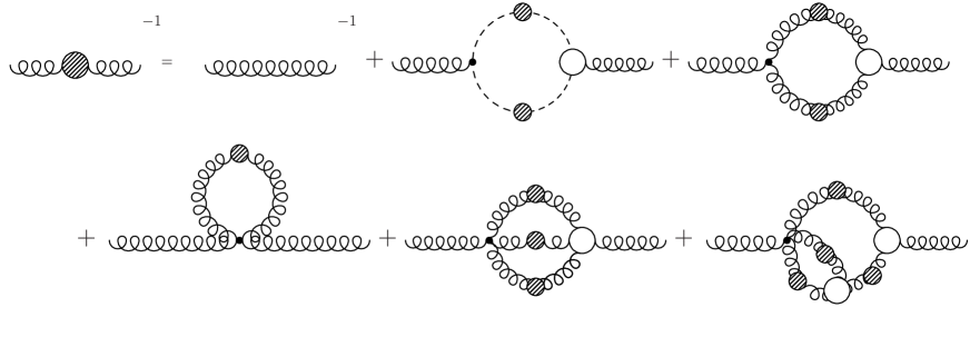
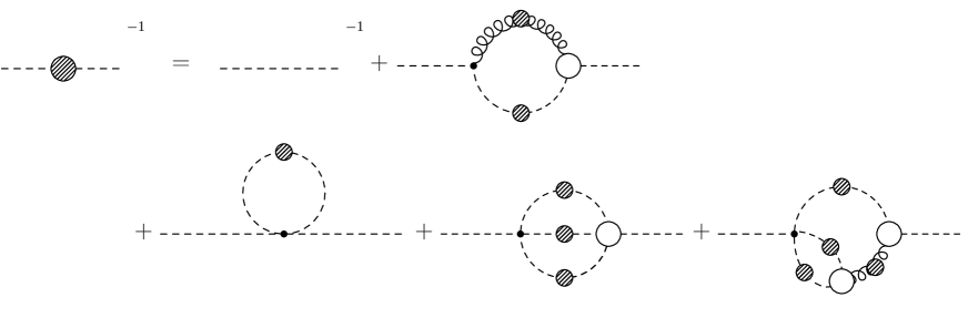
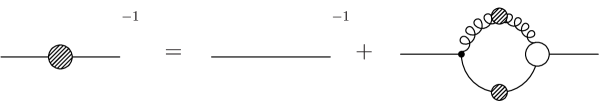
Figure 2.2: The coupled Dyson–Schwinger equations for the gluon, ghost and quark propagators from a BRS and Anti-BRS symmetric Lagrangian. Each of the equations for the gluon and ghost propagators contains genuine one-loop diagrams, a tadpole contribution and a sunset and a squint diagram. All signs and weight factors have been absorbed in the diagrams.

We now perform a Fourier transformation of eq. (LABEL:DSEe_main) and finally introduce renormalisation factors at the appropriate places:

$$[D_{G}(p)]^{-1} = \tilde{Z}_{3}[D_{G}^{(0)}(p)]^{-1}$$

$$- \tilde{Z}_{1}\frac{g^{2}N_{c}}{(2\pi)^{4}}\int d^{4}q\>\Gamma^{(0)}_{\mu}(p,q)\>D_{\mu\nu}(p-q)\>\Gamma_{\nu}(q,p)D_{G}(q)$$

$$- \tilde{Z}_{4}\frac{g^{2}N_{c}}{(2\pi)^{4}}\int d^{4}q\>\Gamma_{4gh}^{(0)}\>D_{G}(q)$$

$$+ \tilde{Z}_{4}\frac{1}{2}\frac{g^{4}N_{c}^{2}}{(2\pi)^{8}}\int d^{4}[q_{1}q_{2}]\Gamma^{(0)}_{4gh}\>D_{G}(q_{1})\>D_{G}(p-q_{1}-q_{2})\>\Gamma_{4gh}(p,q_{1},q_{2})\>D_{G}(q_{2})$$

$$- \tilde{Z}_{4}\frac{1}{4}\frac{g^{4}N_{c}^{2}}{(2\pi)^{8}}\int d^{4}[q_{1}q_{2}]\>\Gamma^{(0)}_{4gh}\>D_{\mu\nu}(p-q_{1})\>D_{G}(q1)\times$$

$$\hskip 85.35826pt\Gamma_{\nu}(p,q_{1})\>D_{G}(q_{2})\>\Gamma_{\mu}(-p+q_{1}+q_{2},q_{2})\>D_{G}(p-q_{1}-q_{2}).$$

The colour traces have already been carried out and the reduced vertices defined in appendix A.3 have been used. The four-ghost interaction generates three new diagrams in the ghost equation, a tadpole contribution and two two-loop diagrams. Furthermore the bare ghost-gluon vertex depends on the gauge parameter $\alpha$,

$$\Gamma_{\mu}^{(0)abc}(k,p,q) = gf^{abc}(2\pi)^{4}\delta^{4}(k+q-p)\Gamma_{\mu}^{(0)}(p,q)$$

$$\Gamma_{\mu}^{(0)}(p,q) = \left[\left(1-\frac{\alpha}{2}\right)q_{\mu}+\frac{\alpha}{2}p_{\mu}\right].$$ (2.79)

Note the symmetry between the ghost momentum $p_{\mu}$ and the antighost momentum $q_{\mu}$, when the gauge parameter $\alpha$ is set to one.

The respective equation for the gluon propagator is formally the same as in the Faddeev-Popov case, where the equations have been derived in ref. [64]. Differences occur in the explicit form of the bare ghost-gluon vertex and the dressed vertices in general depend on the gauge parameters. As the derivation of the DSE from the generating functional brings nothing new we refrain from displaying it explicitly and merely give the result:

$$[D(p)]^{-1}_{\mu\nu} = Z_{3}[D^{(0)}(p)]^{-1}_{\mu\nu}$$

$$+ \tilde{Z}_{1}\frac{g^{2}N_{c}}{(2\pi)^{4}}\int d^{4}q\>\Gamma^{(0)}_{\mu}(p,q)\>D_{G}(p-q)\>\Gamma_{\nu}(q,p)D_{G}(q)$$

$$- Z_{1}\frac{1}{2}\frac{g^{2}N_{c}}{(2\pi)^{4}}\int d^{4}q\>\Gamma^{(0)}_{\mu\rho\sigma}(p,q)\>D_{\rho\rho^{\prime}}(p-q)\>\Gamma_{\rho^{\prime}\nu\sigma^{\prime}}(q,p)D_{\sigma\sigma^{\prime}}(q)$$

$$- Z_{4}\frac{1}{2}\frac{g^{2}N_{c}}{(2\pi)^{4}}\int d^{4}q\>\Gamma^{(0)}_{\mu\nu\rho\sigma}\>D_{\rho\sigma}(q)$$

$$- Z_{4}\frac{1}{6}\frac{g^{4}N_{c}^{2}}{(2\pi)^{8}}\int d^{4}[q_{1}q_{2}]\>\Gamma^{(0)}_{\mu\rho\sigma\lambda}\>D_{\rho\rho^{\prime}}(q_{2})\>D_{\sigma\sigma^{\prime}}(p-q_{2}-q_{1})\times$$

$$\hskip 227.62204pt\Gamma_{\rho^{\prime}\nu\lambda^{\prime}\sigma^{\prime}}(p,q_{1},q_{2})\>D_{\lambda\lambda^{\prime}}(q_{1})$$

$$- Z_{4}\frac{1}{2}\frac{g^{4}N_{c}^{2}}{(2\pi)^{8}}\int d^{4}[q_{1}q_{2}]\>\Gamma^{(0)}_{\mu\rho\sigma\lambda}\>D_{\rho\rho^{\prime}}(p-q_{1}-q_{2})\>D_{\sigma\sigma^{\prime}}(q_{2})\times$$

$$\hskip 56.9055pt\Gamma_{\rho^{\prime}\zeta\sigma^{\prime}}(p-q_{1}-q_{2},q_{2})\>D_{\zeta\zeta^{\prime}}(p-q_{1})\>\Gamma_{\zeta^{\prime}\nu\lambda^{\prime}}(p-q_{1},q_{1})\>D_{\lambda\lambda^{\prime}}(q_{1}).$$

The definitions and conventions for the gluon propagator $D_{\mu\nu}$, the three-gluon vertex $\Gamma_{\mu\nu\rho}$ and the four-gluon vertex $\Gamma_{\mu\nu\rho\sigma}$ are given in appendix A.3.

The Dyson-Schwinger equation for the quark propagator is derived in a similar way from the generating functional and reads explicitly

$$[S(p)]^{-1}=[S^{(0)}(p)]^{-1}-Z_{1F}\frac{g^{2}C_{f}}{(2\pi)^{4}}\int d^{4}q\;\Gamma^{(0)q}_{\mu}(p,q)\;D_{\mu\nu}(p-q)\;S(q)\;\Gamma^{q}_{\mu}(p,q)\;,\hskip 5.69046pt$$ (2.81)

where $S$ denotes the quark propagator and $\Gamma^{q}_{\mu}$ the quark-gluon vertex. The factor $C_{f}=(N_{c}^{2}-1)/(2N_{c})$ stems from the colour trace which has already been carried out.

All three Dyson-Schwinger equations are shown diagrammatically in figure 2.2. One clearly sees the striking similarity between the ghost and the gluon equation once a four-ghost interaction has been introduced. Both equations have bare and one loop parts, a tadpole contribution, a sunset and a squint diagram.

Chapter 3 Propagators of Landau gauge Yang-Mills theory

In this chapter we investigate the Dyson–Schwinger equations for the propagators of Yang–Mills theory. The knowledge of the two point functions of Yang–Mills theory, the ghost and gluon propagator, might shed light on those fundamental properties of QCD, which are generated in the gauge sector (for a recent review see [10]). This is clearly the case for the phenomenon of confinement, as can be inferred from lattice calculations. Furthermore the knowledge of the interaction strength in the gauge sector of QCD provides the basis for a successful description of hadronic physics [10, 9]. Based on the idea of infrared slavery older works on this subject assumed a gluon propagator that is strongly singular in the infrared. Recent studies based either on Dyson–Schwinger equations [66, 67, 68, 69, 62, 70, 18] or Monte-Carlo lattice calculations [71, 72, 73, 65, 74, 75, 76] in Landau gauge indicate quite the opposite: an infrared finite or even infrared vanishing gluon propagator.

Lattice simulations and the Dyson-Schwinger approach are complementary in the following sense: On the one hand, lattice calculations include all non-perturbative physics of Yang–Mills theories but cannot make definite statements about the far infrared due to the finite lattice volume. On the other hand, Dyson–Schwinger equations (DSEs) allow one to extract the leading infrared behaviour analytically and the general non-perturbative behaviour with moderate numerical effort. However, the infinite tower of coupled non-linear integral DSEs has to be truncated in order to be manageable. As we will see in the course of this chapter, the propagators of SU(2) and SU(3) Landau gauge Yang–Mills theory coincide for these two different approaches reasonably well. Thus we are confident that our results for the qualitative features of these propagators are trustworthy.

Throughout this chapter we stay in the framework of ordinary Faddeev–Popov quantisation. Interesting enough, some of our results can be directly compared with recent calculations obtained in a framework employing stochastic quantisation [18]. We will thus be able to check for systematic errors connected to the appearance of Gribov copies [57], c.f. the discussion in section 2.3.3.

Landau gauge, which has been chosen for all DSE studies of Yang-Mills theory so far, is special for a number of reasons. First, it is a fixed point under the renormalisation procedure. This means that the gauge parameter $\lambda$ is not renormalised when $\lambda=0$, a fact which simplifies the renormalisation of the DSEs considerably. Second, as we saw in the last chapter, Landau gauge is a ghost-antighost symmetric gauge. This is of principal interest as we are then allowed to interpret ghost and antighost as (unphysical) particle and antiparticle. On the other hand it simplifies matters if one attempts to construct a non-perturbative dressed ghost-gluon vertex, as one is guided by a symmetry. This has been exploited in references [66, 79, 80]. Third, the ghost-gluon vertex does not suffer from ultraviolet divergences in Landau gauge, as has been shown by Taylor [81]. Again, this simplifies the search for a suitable ansatz for this vertex considerably. Indeed, one is even allowed to use the bare ghost-gluon vertex, as we will see in the course of this chapter.

This chapter is organised as follows: We first give a brief summary of previously employed truncation and approximation schemes for the coupled gluon and ghost DSEs in Landau gauge. We discuss the key role of the ghost-gluon vertex in these truncations and show how a non-perturbative definition of the running coupling can be inferred. One of the obstacles encountered in providing numerical solutions are the angular integrals inherent to these equations. Therefore approximated treatments of the angular integrals have been applied so far [66, 67]. In general these angular approximations proved to be good for high momenta but less trustworthy in the infrared. Recent studies [82, 62, 70] therefore concentrated on the infrared analysis, where exact results have been gained for the limit of vanishing momentum. However, as we will see in the course of this chapter, not every extracted infrared solution is connected to a numerical solution for finite values of momenta. The main part of this chapter is therefore devoted to the construction of a novel truncation scheme, which allows to overcome the angular approximation for the whole range of momenta [83, 84]. Thus we are able to single out the physical infrared solutions of the schemes used in [82, 62, 70]. In the ultraviolet region of momentum we obtain the correct one-loop anomalous dimensions of the propagators known from resummed perturbation theory.

3.1 Gluon and ghost Dyson–Schwinger equations in flat Euclidean space-time

The coupled set of gluon and ghost Dyson–Schwinger equations, which has been given diagrammatically in Fig. 2.2 in the last chapter, loses a considerable amount of complexity in Landau gauge. There, the four-ghost vertex vanishes and we are left with one dressing loop in the ghost equation. As we will only be concerned with pure Yang–Mills theory in this chapter the quark loop in the gluon equation disappears as well. Furthermore in Landau gauge the tadpole term provides an (ultraviolet divergent) constant only and will drop out during renormalisation. Thus we will neglect this contribution from the very beginning. All these simplifications are due to our choice of Landau gauge. The resulting system of equations is still very complicated as it contains full two-loop diagrams in the gluon equation. The first assumption of all truncation schemes up to now is, that contributions from these two-loop diagrams may safely be neglected. We will join in this assumption and provide some arguments for its validity in subsection 3.4.2.

Thus, we will effectively study the coupled system of equations as depicted in Fig. 3.1. The corresponding equations are given by

$$[D_{G}(p)]^{-1} = \tilde{Z_{3}}[D_{G}^{(0)}(p)]^{-1}-\tilde{Z_{1}}\frac{g^{2}N_{c}}{(2\pi)^{4}}\int d^{4}q\>\Gamma^{(0)}_{\mu}(p,q)\>D_{\mu\nu}(p-q)\>\Gamma_{\nu}(q,p)D_{G}(q)\;,\hskip 42.67912pt$$ (3.1)

$${[D(p)]^{-1}_{\mu\nu}} = Z_{3}[D^{(0)}(p)]^{-1}_{\mu\nu}+\tilde{Z_{1}}\frac{g^{2}N_{c}}{(2\pi)^{4}}\int d^{4}q\>\Gamma^{(0)}_{\mu}(p,q)\>D_{G}(p-q)\>\Gamma_{\nu}(q,p)D_{G}(q)$$ (3.2)

$$\hskip 28.45274pt-Z_{1}\frac{1}{2}\frac{g^{2}N_{c}}{(2\pi)^{4}}\int d^{4}q\>\Gamma^{(0)}_{\mu\rho\sigma}(p,q)\>D_{\rho\rho^{\prime}}(p-q)\>\Gamma_{\rho^{\prime}\nu\sigma^{\prime}}(q,p)D_{\sigma\sigma^{\prime}}(q).$$

Here the ghost-gluon vertex is denoted by the symbol $\Gamma_{\nu}(q,p)$, whereas the three-gluon vertex is given by $\Gamma_{\rho\nu\sigma}(q,p)$. Furthermore we have the coupling $g$ and the number of colours $N_{c}$ stemming from the colour trace of the respective loops. Suppressing colour indices the explicit expressions for the ghost and gluon propagators as well as the inverse of the gluon propagator are given by

$$D_{G}(p) = -\frac{G(p^{2})}{p^{2}}\;,$$ (3.3)

$$D_{\mu\nu}(p) = \left(\delta_{\mu\nu}-\frac{p_{\mu}p_{\nu}}{p^{2}}\right)\frac{Z(p^{2})}{p^{2}}+\lambda\frac{p_{\mu}p_{\nu}}{p^{4}}\;,$$ (3.4)

$$\left[D_{\mu\nu}(p)\right]^{-1} = \left(\delta_{\mu\nu}-\frac{p_{\mu}p_{\nu}}{p^{2}}\right)\frac{p^{2}}{Z(p^{2})}+\frac{1}{\lambda}p_{\mu}p_{\nu}\;.$$ (3.5)

For all linear covariant gauges the longitudinal parts of the full and bare inverse gluon propagators cancel each other in the gluon equation (3.2). Furthermore in Landau gauge we have $\lambda=0$.

Figure 3.1: Diagrammatic representation of the truncated Landau gauge gluon and ghost DSEs studied in this chapter. In the gluon Dyson–Schwinger equation terms with four–gluon vertices and quarks have been dismissed.

At this stage of treating the equations we spot a problem: The left hand side of the gluon equation (3.2) is transverse to the gluon momentum therefore the right hand side of this equation should be transverse as well. This is certainly the case in the exact theory. However in an approximate treatment the gluon polarisation on the right hand side may acquire spurious longitudinal terms due to breaking gauge invariance. In general there are two possible sources for this violation: The first one is the use of vertices which violate the corresponding Slavnov-Taylor identity. The second one is the use of a regularisation scheme which breaks gauge invariance, such as a cutoff in the radial momentum integral.

We postpone the problem of the gauge invariance of the vertex ansatz to the next subsection and discuss the regularisation problem first. In the following we outline some rather abstract arguments which will become more transparent in section 3.3, where we investigate the infrared and ultraviolet properties of our new truncation scheme in detail.

In general a cutoff in the loop integrals can lead to quadratically ultraviolet divergent terms in the gluon equation. Such terms are scheme dependent and therefore unphysical. Furthermore they are highly ambiguous because they depend on the momentum routing in the loop integral. Unfortunately, a gauge invariant regularisation scheme avoiding these terms is hard to implement in Dyson–Schwinger studies.

It has been argued though [89, 90], that quadratic divergences can occur only in that part of the right hand side of the equation which is proportional to the metric $\delta_{\mu\nu}$. Therefore an alternative procedure to avoid quadratic divergences is to contract the equation with the tensor [89]

$${\mathcal{R}}_{\mu\nu}(p)=\delta_{\mu\nu}-4\,\frac{p_{\mu}p_{\nu}}{p^{2}}\,,$$ (3.6)

which is constructed such that ${\mathcal{R}}_{\mu\nu}(p)\,\delta^{\mu\nu}=0$. However, as has become obvious recently [70], the use of the tensor (3.6) interferes with the infrared analysis of the coupled gluon-ghost system (see also ref. [91] for a corresponding discussion in a much simpler truncation scheme).

In order to study this problem more carefully we will contract the Lorentz indices of eq. (3.2) with the one-parameter family of tensors

$${\mathcal{P}}^{(\zeta)}_{\mu\nu}(p)=\delta_{\mu\nu}-\zeta\,\frac{p_{\mu}p_{\nu}}{p^{2}}\,.$$ (3.7)

This allows us to interpolate continuously from the tensor (3.6) to the transversal one (with $\zeta=1$). We will then encounter quadratic divergences proportional to the factor $(4-\zeta)$, which can be identified unambiguously and removed by hand. We will be able to show that this procedure restores the correct perturbative behaviour of the equations even with a finite cutoff $\Lambda$.

Having removed all quadratic divergences we are then in a position to evaluate the remaining degree of breaking gauge invariance. As a completely transversal right hand side would be independent of $\zeta$ after contraction with the projector (3.7), the variation of our solutions with $\zeta$ is a measure for the influence of the artificial longitudinal terms on the right hand side of the equation.

3.2 The ghost-gluon vertex in DSE studies and the running coupling

We now focus on two issues that are connected with the ghost-gluon vertex of Landau gauge. We will argue for the surprising fact, that one can safely use a bare ghost-gluon vertex even in the non-perturbative momentum region of the DSEs. Furthermore we describe, how one is able to relate the running coupling of the strong interaction to the ghost and gluon dressing functions by the renormalisation properties of the ghost-gluon vertex.

3.2.1 Dressing the ghost-gluon vertex

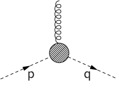
Figure 3.2: A diagrammatical representation of the ghost-gluon vertex.

For our further treatment of the ghost and gluon system of equations, (3.1) and (3.2), we have to specify explicit forms for the dressed ghost-gluon vertex $\Gamma_{\nu}(q,p)$ and the dressed three-gluon vertex $\Gamma_{\rho\nu\sigma}(q,p)$. As has already been mentioned in the introduction to this chapter, the ghost-gluon vertex does not attribute an independent ultraviolet divergence in Landau gauge, i.e. one has $\widetilde{Z}_{1}=1$ [81]. Therefore a truncation based on the tree-level form for the ghost-gluon vertex function,

$$\Gamma_{\mu}(q,p)=iq_{\mu}$$ (3.8)

is compatible with the desired short distance behaviour of the solutions. Here the momentum $q_{\mu}$ is the momentum of the outgoing ghost, see Fig. 3.2. Thus we obtain the correct ultraviolet behaviour of the ghost loop in the gluon equation (3.2) and the dressing loop in the ghost equation (3.1), as will be shown explicitly below.

However, as the effects of non-perturbative vertex dressing are supposed to be most pronounced in the infrared, one might wonder whether the tree-level form of the ghost-gluon vertex leads to a sensible infrared behaviour of these equations. Furthermore the bare vertex violates the Slavnov-Taylor identity (STI), which restricts that part of the ghost-gluon vertex which is longitudinal in the gluon momentum. Such an identity is the manifestation of gauge invariance and can be derived using the BRS-invariance of the gauge-fixed Lagrangian of Yang–Mills theory.

Considering this, obviously the best way to obtain a properly dressed ansatz for the ghost-gluon vertex is to solve the corresponding STI. This strategy has been followed by von Smekal, Hauck and Alkofer in [66, 79]. On the level of connected Green’s functions the STI for the ghost-gluon vertex in general linear covariant gauges reads [79]

$$\frac{1}{\lambda}\langle c^{c}(z)\bar{c}^{b}(y)\partial A^{a}(x)\rangle-\frac{1}{\lambda}\langle c^{c}(z)\bar{c}^{a}(x)\partial A^{b}(y)\rangle=-\frac{g}{2}f^{cde}\langle c^{d}(z)c^{e}(z)\bar{c}^{a}(x)\bar{c}^{b}(y)\rangle.$$ (3.9)

Here we have the spatial coordinates $x$, $y$ and $z$, the bare coupling $g$, the gauge parameter $\lambda$ and the real structure constant $f^{cde}$ of the gauge group SU(3). The left hand side of this equation can be decomposed into the full ghost-gluon vertex and respective propagators. However, the right hand side contains the connected ghost-ghost scattering kernel, which is completely unknown.

By neglecting this irreducible correlation von Smekal, Hauck and Alkofer were able to construct a vertex ansatz which solves the resulting approximate STI. Together with a similar construction for the three-gluon vertex they obtained a closed system of equations which has been solved numerically using an angular approximation (c.f. subsection 5.1.1). The results, an infrared vanishing gluon propagator and an highly singular ghost in the infrared have been confirmed since in other DSE-calculations as well as lattice Monte-Carlo simulations [71, 72, 73, 65]. Thus the old idea of infrared slavery based on the notion of an infrared divergent gluon propagator has been abandoned since.

However, as became clear later, the vertex construction of refs. [66, 79] is somewhat problematic. It has been shown in ref. [67] that this vertex causes inconsistencies in the infrared behaviour of the ghost equation once the angular integrals of the dressing loop are treated exactly. Furthermore it has been shown in refs. [92, 93] that the neglection of the irreducible ghost-ghost scattering kernel in the identity (3.9) is at odds with perturbation theory. On the other hand it is hard to see, how one could include this irreducible correlation and thus improve the construction of refs. [66, 79].

Therefore Atkinson and Bloch chose a different strategy and employed a bare ghost-gluon vertex in their truncation scheme [67, 82], which keeps only the ghost loop in the gluon equation. The numerical calculations in this scheme are also obtained using angular approximations in the integrals. Amazingly, though, the bare vertex scheme and the one from [66, 79] provide results with qualitatively similar infrared behaviour: the gluon propagator vanishes in the infrared and the ghost propagator is highly singular there.

The surprising conclusion from the comparison of these two truncation schemes is, that a bare ghost-gluon vertex (3.8) is not only capable of providing the correct ultraviolet behaviour of the ghost loop in the gluon equation (3.2) and the dressing loop in the ghost equation (3.1), but in addition leads to a satisfactory infrared behaviour of the equations in accordance with lattice Monte–Carlo simulations. Consequently recent analytical infrared investigations concentrated on the bare vertex [82, 62]. The influence of multiplicative corrections to the bare vertex has been assessed in refs. [70, 94] and are found to be irrelevant for the qualitative behaviour in the infrared.

For our novel truncation scheme, detailed in section 3.3, we will therefore use the bare ghost-gluon vertex (3.8), keeping in mind that we have to check for the influence of artificial longitudinal terms due to the violation of the Slavnov-Taylor identity (3.9). As a major improvement to previous calculations we will be able to overcome the angular approximation and give solutions for the ghost and gluon dressing functions which include the full angular dependence of the loops in the equations.

3.2.2 The running coupling of the strong interaction

Before we give the details of our truncation scheme there is still more to be learned from the ghost-gluon vertex in Landau gauge. In the following we consider the renormalisation of the vertex term in the unrenormalised Lagrangian, eq. (2.11). In Landau gauge we have

$${\cal{L}}_{ghost-gluon}=gf^{abc}\partial_{\mu}\bar{c}^{a}A_{\mu}^{c}c^{b}\;,$$ (3.10)

which is identical to the respective term in the Faddeev-Popov Lagrangian, eq. (2.10). Multiplicative renormalisability means that it is possible to render all Green’s functions finite by renormalising the fields and parameters of the Lagrangian without changing its form. Recall that the coupling $g$, the gluon field and the ghost field are renormalised according to (c.f. eq. (2.13))

$$A_{\mu}^{a} \rightarrow \sqrt{Z_{3}}A_{\mu}^{a}\,,$$ (3.11)

$$\bar{c}^{a} \rightarrow \sqrt{\tilde{Z}_{3}}\bar{c}^{a}\,,$$ (3.12)

$$c^{a} \rightarrow \sqrt{\tilde{Z}_{3}}c^{a}\,,$$ (3.13)

$$g \rightarrow Z_{g}g\,,$$ (3.14)

where we have unrenormalised objects on the left hand side and renormalised ones of the right hand side of the relations. Furthermore, by definition, the vertex renormalisation constant $\tilde{Z}_{1}$ is related to the renormalisation constants of the constituent fields of the vertex by

$$\tilde{Z}_{1}=Z_{g}\tilde{Z}_{3}Z_{3}^{1/2}.$$ (3.15)

We then have the renormalised ghost-gluon vertex part of the Lagrangian

$${\cal{L}}_{ghost-gluon}^{R}=\tilde{Z}_{1}gf^{abc}\partial_{\mu}\bar{c}^{a}A_{\mu}^{c}c^{b}\,,$$ (3.16)

which has the same form as the respective term (3.10) in the bare Lagrangian.

We are now able to exploit the fact again that $\tilde{Z}_{1}=1$ in Landau gauge [81]. As the strong running coupling is defined by $\alpha=g^{2}/(4\pi)$, we obtain the relation

$$\alpha(\Lambda^{2})=\frac{\alpha(\mu^{2})}{\tilde{Z}_{3}^{2}(\mu^{2},\Lambda^{2})Z_{3}(\mu^{2},\Lambda^{2})}$$ (3.17)

from the renormalisation of the coupling, eq. (3.14). Here we gave the explicit arguments of the renormalised coupling $\alpha(\mu^{2})$, evaluated at the renormalisation point $\mu$, and the bare coupling $\alpha(\Lambda^{2})$, which depends on the cutoff $\Lambda$ of our theory. From the relations (3.11) and (3.13) we furthermore infer that the ghost and gluon dressing functions, $G(p^{2})$ and $Z(p^{2})$, are renormalised according to

$$G(p^{2},\Lambda^{2}) = G(p^{2},\mu^{2})\,\tilde{Z}_{3}(\mu^{2},\Lambda^{2})\,,$$

$$Z(p^{2},\Lambda^{2}) = Z(p^{2},\mu^{2})\,{Z}_{3}(\mu^{2},\Lambda^{2})\,,$$ (3.18)

where the unrenormalised quantities are on the left hand side of the equations. Certainly the renormalisation point $\mu$ is completely free. We are thus allowed to substitute these relations into eq. (3.17) and renormalise once at an arbitrary point $\mu$ and once at the specific value $p$. We obtain

$$\alpha(\Lambda^{2})\,G^{2}(p^{2},\Lambda^{2})\,Z(p^{2},\Lambda^{2})=\alpha(\mu^{2})\,G^{2}(p^{2},\mu^{2})\,Z(p^{2},\mu^{2})=\alpha(p^{2})\,G^{2}(p^{2},p^{2})\,Z(p^{2},p^{2})$$ (3.19)

It suffices now to impose the non-perturbative renormalisation condition

$$G^{2}(p^{2},p^{2})\,Z(p^{2},p^{2})=G^{2}(\mu^{2},\mu^{2})\,Z(\mu^{2},\mu^{2})=1$$ (3.20)

on equation (3.19) to arrive at

$$\framebox{$\displaystyle\alpha(p^{2})=\alpha(\mu^{2})\,G^{2}(p^{2},\mu^{2})\,Z(p^{2},\mu^{2})$}$$ (3.21)

This is a defining equation for the non-perturbative running coupling $\alpha(p^{2})$ of Landau gauge QCD [66, 79]. Note that the running coupling $\alpha(p^{2})$ defined this way does not depend on the arbitrary renormalisation point $\mu$. This is equivalent to saying that the right hand side of this equation is a renormalisation group invariant [95].

3.3 The truncation scheme

Having spent some time with the discussion of Landau gauge we now return to the coupled set of eqs. (3.1) and (3.2) and specify explicit expressions for the ghost-gluon vertex $\Gamma_{\nu}(q,p)$ and the three-gluon vertex $\Gamma_{\rho\nu\sigma}(q,p)$. In the following we will show, that the bare ghost-gluon vertex

$$\Gamma_{\mu}(q,p)=iq_{\mu}$$ (3.22)

and the construction

$$\Gamma_{\rho\nu\sigma}(q,p)=\frac{1}{Z_{1}(\mu^{2},\Lambda^{2})}\,\frac{G(q^{2})^{(1-a/\delta-2a)}}{Z(q^{2})^{(1+a)}}\frac{G((q-p)^{2})^{(1-b/\delta-2b)}}{Z((q-p)^{2})^{(1+b)}}\,\Gamma^{(0)}_{\rho\nu\sigma}(q,p)$$ (3.23)

with the bare three-gluon vertex $\Gamma^{(0)}_{\rho\nu\sigma}$ given in eq. (A.31) and the new parameters $a$ and $b$ lead to the correct one-loop anomalous dimensions of the dressing functions in the ultraviolet, provided the quadratic divergences have been removed. This is true for arbitrary values of the parameters $a$ and $b$, although we will later argue for the specific values $a=b=3\delta$, where $\delta$ is the anomalous dimension of the ghost.

For simplicity we introduce the abbreviations $x:=p^{2}$, $y:=q^{2}$ and $z:=k^{2}=(q-p)^{2}$ for the squared momenta appearing as arguments of the dressing functions. Furthermore $s:=\mu^{2}$ and $L:=\Lambda^{2}$ denote the squared renormalisation point and the squared momentum cutoff of the theory. Substituting the two vertices in the ghost and gluon system (3.1) and (3.2) we then arrive at

$$\frac{1}{G(x)} = \tilde{Z}_{3}-g^{2}N_{c}\int\frac{d^{4}q}{(2\pi)^{4}}\frac{K(x,y,z)}{xy}G(y)Z(z)\;,$$ (3.24)

$$\frac{1}{Z(x)} = {Z}_{3}+g^{2}\frac{N_{c}}{3}\int\frac{d^{4}q}{(2\pi)^{4}}\frac{M(x,y,z)}{xy}G(y)G(z)$$ (3.25)

$$\hskip 17.07182pt+g^{2}\frac{N_{c}}{3}\int\frac{d^{4}q}{(2\pi)^{4}}\frac{Q(x,y,z)}{xy}\frac{G(y)^{(1-a/\delta-2a)}}{Z(y)^{a}}\frac{G(z)^{(1-b/\delta-2b)}}{Z(z)^{b}}\;.$$

The kernels ordered with respect to powers of $z$ have the form:

$$K(x,y,z) = \frac{1}{z^{2}}\left(-\frac{(x-y)^{2}}{4}\right)+\frac{1}{z}\left(\frac{x+y}{2}\right)-\frac{1}{4}\,,$$

$$M(x,y,z) = \frac{1}{z}\left(\frac{\zeta-2}{4}x+\frac{y}{2}-\frac{\zeta}{4}\frac{y^{2}}{x}\right)+\frac{1}{2}+\frac{\zeta}{2}\frac{y}{x}-\frac{\zeta}{4}\frac{z}{x}\,,$$

$$Q(x,y,z) = \frac{1}{z^{2}}\left(\frac{1}{8}\frac{x^{3}}{y}+x^{2}-\frac{19-\zeta}{8}xy+\frac{5-\zeta}{4}y^{2}+\frac{\zeta}{8}\frac{y^{3}}{x}\right)$$ (3.26)

$$+\frac{1}{z}\left(\frac{x^{2}}{y}-\frac{15+\zeta}{4}x-\frac{17-\zeta}{4}y+\zeta\frac{y^{2}}{x}\right)$$

$$-\left(\frac{19-\zeta}{8}\frac{x}{y}+\frac{17-\zeta}{4}+\frac{9\zeta}{4}\frac{y}{x}\right)+z\left(\frac{\zeta}{x}+\frac{5-\zeta}{4y}\right)+z^{2}\frac{\zeta}{8xy}\,.\hskip 14.22636pt$$

3.3.1 Ultraviolet analysis

In order to identify the quadratically divergent terms in the kernels $K$, $M$ and $Q$ we now analyse eqs. (3.24) and (3.25) in the limit of large momenta $x$. It is known from resummed perturbation theory (see e.g. [6]) that the behaviour of the dressing functions for large Euclidean momenta can be described as

$$Z(x) = Z(s)\left[\omega\log\left(\frac{x}{s}\right)+1\right]^{\gamma}\;,$$ (3.27)

$$G(x) = G(s)\left[\omega\log\left(\frac{x}{s}\right)+1\right]^{\delta}\;.$$ (3.28)

Here $Z(s)$ and $G(s)$ denote the value of the dressing functions at some renormalisation point $s:=\mu^{2}$ and $\gamma$ and $\delta$ are the respective anomalous dimensions. To one loop one has $\delta=-9/44$ and $\gamma=-1-2\delta=-13/22$ for arbitrary number of colours $N_{c}$ and no quarks, $N_{f}=0$. Furthermore, $\omega={11N_{c}}\alpha(s)/{12\pi}$.

The slowly varying logarithmic behaviour of the dressing functions in the ultraviolet justifies the angular approximation

$$Z(z),G(z)\longrightarrow Z(y),G(y)\hskip 28.45274pt\mbox{for}\>\>\>y>x$$ (3.29)

in the ultraviolet. The angular integrals in eqs. (3.24) and (3.25) can then be trivially calculated using the angular integration formulae of appendix C.1. Furthermore, as the cutoff $L=\Lambda^{2}$ can be chosen arbitrary large, the integrals will be dominated by the part from $x$ to $L$. We then obtain

$$\frac{1}{G(x)} = \tilde{Z}_{3}-g^{2}\frac{N_{c}}{16\pi^{2}}\int\frac{dy}{x}\frac{3}{4y}G(y)Z(y)\;,$$ (3.30)

$$\frac{1}{Z(x)} = {Z}_{3}+g^{2}\frac{N_{c}}{48\pi^{2}}\int\frac{dy}{x}\left[\left(\frac{4-\zeta}{4}+\frac{\zeta-2}{4}\frac{x}{y}\right)G^{2}(y)\right.$$ (3.31)

$$\hskip 56.9055pt+\left.\left(\frac{-3(4-\zeta)}{2}-\frac{\zeta+24}{4}\frac{x}{y}+\frac{7}{8}\frac{x^{2}}{y^{2}}\right)\frac{G(y)^{(2-(a+b)/\delta-2(a+b))}}{Z(y)^{(a+b)}}\right]\,.\hskip 22.76228pt$$

We are now able to identify the quadratic divergences in the gluon equation, which are the two terms independent of the integration momentum. Both, the one from the ghost loop and the one from the gluon loop, are proportional to $(4-\zeta)$ and therefore vanish when we use the Brown-Pennington projector, eq. (3.6). For general values of $\zeta$ we have to subtract these terms by hand. However, this cannot be done straightforwardly at the level of integrands: Such a procedure would disturb the infrared properties of the Dyson–Schwinger equations. Since we anticipate from previous studies and analytic work [62, 70] that the ghost loop is the leading contribution in the infrared the natural place to subtract the quadratically ultraviolet divergent constant is the gluon loop. We do this by employing the substitution

$$Q(x,y,z)\,\,\to\,\,\tilde{Q}(x,y,z)=Q(x,y,z)+\frac{5}{4}(4-\zeta)$$ (3.32)

in eq. (3.25). Only the problematic terms in eq. (3.31) then disappear.

Having subtracted the quadratic divergences from the ghost and gluon system we now check for the logarithmic divergences, which should match to perturbation theory. We choose the perturbative renormalisation condition $G(s)=Z(s)=1$ at a large Euclidean renormalisation point $s=\mu^{2}$ and plug the perturbative expressions (3.27) and (3.28) in eqs. (3.30), (3.31). Thus we arrive at

$$\left[\omega\log\left(\frac{x}{s}\right)+1\right]^{-\delta} = \tilde{Z}_{3}-\frac{3N_{c}g^{2}}{64\pi^{2}\omega(\gamma+\delta+1)}\times$$

$$\hskip 22.76228pt\left\{\left[\omega\log\left(\frac{L}{s}\right)+1\right]^{\gamma+\delta+1}-\left[\omega\log\left(\frac{x}{s}\right)+1\right]^{\gamma+\delta+1}\right\}\,,\hskip 25.6073pt$$

$$\left[\omega\log\left(\frac{x}{s}\right)+1\right]^{-\gamma} = Z_{3}+\left(\frac{N_{c}g^{2}}{96\pi^{2}\omega(2\delta+1)}-\frac{7N_{c}g^{2}}{48\pi^{2}\omega(2\delta+1)}\right)\times$$ (3.33)

$$\hskip 22.76228pt\left\{\left[\omega\log\left(\frac{L}{s}\right)+1\right]^{2\delta+1}-\left[\omega\log\left(\frac{x}{s}\right)+1\right]^{2\delta+1}\right\}\,.$$

Note that these equations are completely independent of the parameters $a$ and $b$ in the three-gluon vertex, eq. (3.23). Note also, that the ultraviolet behaviour of the equations is independent of the parameter $\zeta$ in the projector (3.7). We are therefore left with a transversal structure in the gluon equation for ultraviolet momenta. The renormalisation constants $Z_{3}(s,L)$ and $\tilde{Z}_{3}(s,L)$ cancel the cutoff dependence, i.e. the respective first terms in the brackets. Thus, the power and the prefactor of the second term have to match with the left hand side of the equations. This leads to three conditions:

$$\gamma+2\delta+1 = 0\;,$$ (3.34)

$$\frac{3}{4(\gamma+\delta+1)}\frac{N_{c}g^{2}}{16\pi^{2}\omega} = 1\;,$$ (3.35)

$$\frac{13}{6\>(2\delta+1)}\frac{N_{c}g^{2}}{16\pi^{2}\omega} = 1\;.$$ (3.36)

Eq. (3.34) is of course nothing else but consistency of the ghost equation with one-loop scaling. All three equations together result in the correct anomalous dimensions $\gamma=-13/22$ and $\delta=-9/44$ for an arbitrary number of colours and zero flavours.

Having established this result let us pause for a moment and reflect our construction (3.23) for the three-gluon vertex. There are two possible ways to obtain this construction and we leave it to the taste of the reader which philosophy to prefer. The first way to see eq. (3.23) is to take it at face value as a minimally dressed vertex ansatz, constructed in such a way as to obtain the correct one-loop scaling of the gluon loop. Then the parameters $a$ and $b$ are completely free. Note that the choice $a=b=0$ corresponds to the truncation scheme of [85] whereas $a=3\delta,b=0$ together with the appropriate vertex dressings reproduces case c) of ref. [66].

The second point of view, which is to be found in reference [66], is to employ a bare three-gluon vertex, $\Gamma^{0}_{\rho\nu\sigma}(q,p)$, and then ask the question how the renormalisation constant $Z_{1}$ has to behave, given that the theory should have the correct perturbative limit. Certainly, as both vertices violate their respective Slavnov-Taylor identities, there is no reason why the vertex renormalisation constant $Z_{1}$ should obey the corresponding identity $Z_{1}=Z_{3}/\tilde{Z}_{3}$. For the present truncation scheme the answer is, that the constant $Z_{1}$ acquires a momentum dependence according to

$$Z_{1}\;\;\longrightarrow\;\;{\mathcal{Z}}_{1}(x,y,z;s)=\frac{G(y,s)^{(1-a/\delta-2a)}}{Z(y,s)^{(1+a)}}\frac{G(z,s)^{(1-b/\delta-2b)}}{Z(z,s)^{(1+b)}}\,.$$ (3.37)

This is precisely the form required to transform our vertex (3.23) to the bare one and nevertheless obtain eqs. (3.24) and (3.25).

A reasonable choice of parameters is then one which keeps ${\mathcal{Z}}_{1}$ as weakly dependent as possible on the momenta $y$ and $z$, c.f. Fig. C.2 in appendix C.5. The infrared behaviour of the gluon loop in the gluon equation depends strongly on $a$ and $b$. Setting $b=0$ one can distinguish three cases: For $a<0$ the gluon loop is subleading in the infrared, for $a=0$ as in ref. [85] the gluon loop produces the same power as the ghost loop, for $a>0$ the gluon loop becomes the leading term in the infrared. In the latter case we did not find a solution to the coupled gluon-ghost system. In Appendix C.5 we demonstrate that $a=b=3\delta$ minimises the momentum dependence of ${\mathcal{Z}}_{1}$. Thus we use these values except stated otherwise explicitly.

3.3.2 Infrared analysis

The leading infrared behaviour of the propagator functions in this truncation scheme for the special case of the transverse projector ($\zeta=1$) has been determined recently [62, 70]. Our analysis in this subsection is valid for general values of the parameter $\zeta$ and furthermore includes subleading contributions [84]. The general assumption at the beginning of all analytic infrared investigations is, that the ghost and gluon dressing functions, G and Z, behave like power laws in the infrared:

$$Z(x) = Ax^{\kappa_{1}},$$

$$G(x) = Bx^{\kappa_{2}}.$$ (3.38)

This assumption is justified, if we are able to show that the ansatz (3.38) solves the ghost and gluon system, eqs. (3.24), (3.25), self-consistently in the infrared. As all loop integrals in the equations are dominated by contributions around the external momentum $x=p^{2}$, we are allowed to substitute the power laws for the whole momentum range up to the cutoff $L=\Lambda^{2}$. Errors due to this approximation are subleading in the infrared. Furthermore, as has been shown in detail in reference [70], the renormalisation constants $Z_{3}$ and $\tilde{Z}_{3}$ can be dropped for very small momenta $x$: They are either subleading in the infrared (gluon equation) or have to be zero when the renormalisation takes place at $\mu=0$ (ghost equation). We will explain this point more precisely later on. Plugging the power laws (3.38) into eqs. (3.24), (3.25) we then arrive at

$$\frac{1}{Bx^{\kappa_{2}}} = -g^{2}N_{c}AB\int\frac{d^{4}q}{(2\pi)^{4}}\frac{K(x,y,z)}{xy}z^{\kappa_{1}}y^{\kappa_{2}}\,,$$ (3.39)

$$\frac{1}{Ax^{\kappa_{1}}} = g^{2}\frac{N_{c}}{3}B^{2}\int\frac{d^{4}q}{(2\pi)^{4}}\frac{M(x,y,z)}{xy}y^{\kappa_{2}}z^{\kappa_{2}}$$ (3.40)

$$+g^{2}\frac{N_{c}}{3}B^{-4-12\delta}A^{-6\delta}\int\frac{d^{4}q}{(2\pi)^{4}}\frac{\tilde{Q}(x,y,z)}{xy}y^{(-2-6\delta){\kappa_{2}}-3\delta{\kappa_{1}}}z^{(-2-6\delta){\kappa_{2}}-3\delta{\kappa_{1}}}\,,\hskip 22.76228pt$$

with the kernels $K$, $M$ and $\tilde{Q}$ given by eqs. (3.26), (3.32) and the parameters $a=b=3\delta$ as motivated in the last subsection.

We first investigate the ghost equation (3.39). Shifting the cutoff $L=\Lambda^{2}$ to infinity we are able to use the formula [70]

$$\int d^{4}q\>y^{a}z^{b}=\pi^{2}x^{2+a+b}\frac{\Gamma(2+a)\Gamma(2+b)\Gamma(-a-b-2)}{\Gamma(-a)\Gamma(-b)\Gamma(4+a+b)}$$ (3.41)

for the integration of the dressing loop on the right hand side of the equation. The straightforward but tedious algebra is done with the help of the algebraic manipulation program FORM [96]. We obtain

$$\frac{1}{Bx^{\kappa_{2}}} = -x^{\kappa_{1}+\kappa_{2}}\>\frac{g^{2}N_{c}AB}{16\pi^{2}}\frac{3}{2\,(\kappa_{1}+\kappa_{2})\,(-1+\kappa_{1}+\kappa_{2})}\times$$ (3.42)

$$\hskip 142.26378pt\times\frac{\Gamma(2-\kappa_{1}-\kappa_{2})\,\Gamma(1+\kappa_{1})\,\Gamma(2+\kappa_{2})}{\Gamma(3+\kappa_{1}+\kappa_{2})\,\Gamma(2-\kappa_{1})\,\Gamma(1-\kappa_{2})}.\hskip 28.45274pt{}$$

Matching powers of $x$ on both sides of the equation we arrive at the condition

$$\kappa_{1}=-2\kappa_{2}\;.$$ (3.43)

With the definition $\kappa:=-\kappa_{2}$ we thus have from eqs. (3.38) the power laws

$$\framebox{$\displaystyle\begin{array}[]{c}Z(x)=Ax^{2\kappa},\\ G(x)=Bx^{-\kappa}.\end{array}$}$$ (3.44)

Our derivation of these power laws used the special form of a bare ghost-gluon vertex. It has been shown, however, that relation (3.43) holds under the general assumption that the ghost-gluon vertex can be expanded in a power series [68]. We thus have the interesting situation that the infrared divergence of one of our dressing functions, $Z$ or $G$, is always connected to the vanishing of the other. This has interesting consequences for the running coupling $\alpha(x)$. Recall the definition

$$\alpha(x)=\alpha(s)\,G^{2}(x,s)\,Z(x,s)$$ (3.45)

from eq. (3.21) with $x=p^{2}$ and $s=\mu^{2}$ and $\alpha(s)=g^{2}/{4\pi}$. Substituting the power laws (3.44) we obtain

$$\alpha(0)=\frac{g^{2}}{4\pi}AB^{2}.$$ (3.46)

The coupling approaches a finite value in the infrared. Within the framework of Dyson-Schwinger studies such a behaviour of the running coupling has first been found in ref. [66]. An infrared fixed point is also found in the flow equation study in ref. [97] and analytic perturbation theory [98, 99, 100, 101].

Consider now the gluon equation (3.40). After some algebra using formula (3.41) we find, that the ghost loop is proportional to $x^{2\kappa_{2}}$, whereas the gluon loop is subleading in the infrared. We thus again obtain relation (3.43), $\kappa_{1}=-2\kappa_{2}$, as matching condition for the ghost loop and the leading power on the left hand side of the equation in the infrared. Together with eq. (3.42) we arrive at the two conditions

$$\frac{1}{18}\frac{(2+\kappa)(1+\kappa)}{(3-2\kappa)} = \frac{\Gamma^{2}(2-\kappa)\Gamma(2\kappa)}{\Gamma(4-2\kappa)\Gamma^{2}(1+\kappa)}\>\frac{g^{2}N_{c}}{48\pi^{2}}{AB^{2}}\;,$$ (3.47)

$$\frac{4\kappa-2}{4\zeta\kappa-4\kappa+6-3\zeta} = \frac{\Gamma^{2}(2-\kappa)\Gamma(2\kappa)}{\Gamma(4-2\kappa)\Gamma^{2}(1+\kappa)}\>\frac{g^{2}N_{c}}{48\pi^{2}}{AB^{2}}\;.$$ (3.48)

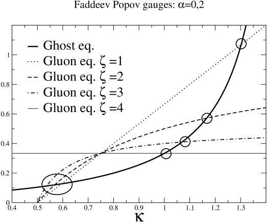
Figure 3.3: Here the graphical solution to equations (3.47) and (3.48) is shown. The thick line represents the left hand side of equation (3.47), whereas the other four curves depict the left hand side of equation (3.48) for different values of the parameter $\zeta$. The ellipse marks the bulk of solutions between $\kappa=0.5$ and $\kappa=0.6$ for different $\zeta$, whereas the circles show the movement of the solution $\kappa=1.3$ for a transverse projector to $\kappa=1$ for the Brown-Pennington case, $\zeta=4$.

from the ghost and gluon equations in the infrared. Equating both left and right hand sides we are able to determine $\kappa$, see Fig. 3.3. For the Brown–Pennington projector, i.e. $\zeta=4$, one then finds the known solution $\kappa=1$ [67]. However, as can be seen immediately, the left hand side of the second equation possesses a zero for $\kappa=1/2$ which is cancelled by a pole only for $\zeta=4$. Lowering $\zeta$ only slightly a further solution with $\kappa$ slightly larger than 0.5 exists. For the transverse projector, i.e. $\zeta=1$, this latter solution becomes

$$\kappa=\frac{93-\sqrt{1201}}{98}\approx 0.595353$$ (3.49)

in accordance with refs. [62, 70]. Also the solution $\kappa=1$ changes continuously when lowering $\zeta$. The corresponding $\kappa$ are then all larger than 1 and contradict the masslessness condition, see section 5.2 of ref. [10] for a discussion of this condition. One of the main results of the numerical section of this chapter is that the infrared behaviour $\kappa\approx 0.5$ matches to a numerical solution whereas no numerical solutions could be found with the infrared behaviour $\kappa\geq 1$. This is in perfect accordance with the Kugo-Ojima criterion and Zwanziger’s horizon condition discussed in section 2.3.

Now let us come back again to the running coupling, eq. (3.45). As can be seen directly from eqs. (3.47), (3.48), the product $N_{c}g^{2}AB^{2}$ is constant for given $\kappa$. With $\alpha(0)={g^{2}}AB^{2}/{4\pi}$ one concludes immediately that $\alpha(x)$ is proportional to $N_{c}^{-1}$. Furthermore, the ghost and gluon dressing functions $Z(x)$ and $G(x)$ are independent of the number of colours: $N_{c}$ enters the Dyson-Schwinger equations only in the combination $g^{2}N_{c}$ at our level of truncation. From the solution $\kappa=0.595$ of the infrared analysis with the transverse projector $\zeta=1$ one determines the infrared fixed point of the running coupling to be

$$\alpha(0)=\frac{2\pi}{3\,N_{c}}\frac{\Gamma(3-2\kappa)\;\Gamma(3+\kappa)\;\Gamma(1+\kappa)}{\Gamma^{2}(2-\kappa)\;\Gamma(2\kappa)}\approx 8.915/N_{c}$$ (3.50)

for general numbers of colours $N_{c}$.

Having determined the leading infrared behaviour of the ghost and gluon system we now check for subleading contributions, and judge their importance for the numerical treatment of the coupled system of equations. An obvious extension of the power law (3.44) is the ansatz

$$Z(x) = Ax^{2\kappa}(1+fx^{\rho})$$

$$G(x) = Bx^{-\kappa}(1+gx^{\rho})$$ (3.51)

which is substituted in the eqs. (3.24) and (3.25). After integration the conditions on the leading term remain unchanged. Matching subleading powers leads to the coupled set of homogeneous equations for $f,g$ and $\rho$:

$$\left(3\nu\frac{6\kappa\,(\kappa-1)\,(-3+2\kappa)}{(\kappa+\rho-2)\,(\kappa+\rho-1)\,(\kappa+\rho)}\frac{\Gamma(2\kappa)\,\Gamma(2-\kappa+\rho)\,\Gamma(3-\kappa-\rho)}{\Gamma(4-2\kappa)\,\Gamma(1+\kappa-\rho)\,\Gamma(3+\kappa+\rho)}-1\right)g$$

$$+\left(3\nu\frac{3\,(-2+2\kappa+\rho)}{2\,(\kappa+\rho-2)\,(\kappa+\rho-1)\,(\kappa+\rho)}\frac{\Gamma(2-\kappa)\,\Gamma(2\kappa+\rho+1)\,\Gamma(3-\kappa-\rho)}{\Gamma(3-2\kappa-\rho)\,\Gamma(1+\kappa)\,\Gamma(3+\kappa+\rho)}\right)f = 0\;,$$

$$\left(\nu\frac{4\zeta\kappa-4\kappa+2\rho-2\zeta\rho+6-3\alpha}{2\kappa-\rho-1}\frac{\Gamma(2-\kappa)\,\Gamma(2\kappa-\rho)\,\Gamma(2-\kappa+\rho)}{\Gamma(1+\kappa)\,\Gamma(1+\kappa-\rho)\,\Gamma(4-2\kappa+\rho)}\right)g+f = 0\;.$$

Here $\nu={N_{c}g^{2}AB^{2}}/{48\pi^{2}}={\alpha(0)}/{4\pi}$. There is either the trivial solution $f=g=0$ or one has to set the determinant of these linear equations to zero. We then obtain the results $\rho_{(1)}=0,\rho_{(2)}=0.58377,\rho_{(3)}=1.20300$ and several other solutions with higher values of the power. The solution $\rho_{(1)}=0$ corresponds to the pure power solution. The lowest non-vanishing solution, $\rho_{(2)}=0.58377$, is sufficiently high that we safely may neglect it in the numerical treatment of the infrared part of the equations. This will be detailed in the next section.

Finally, let us come back to the role of the renormalisation constants $\tilde{Z}_{3}$ and ${Z}_{3}$ in eq. (3.39), (3.40). There are two possible situations, which have been clarified in [70]. First, consider an infrared vanishing dressing function, as is the case in the gluon equation. Then the left hand side of eq. (3.40) as well as the loop integral on the right hand side are diverging, and the $x$-independent constant ${Z}_{3}$ is subleading and therefore negligible in the infrared. Second, in the ghost equation we have the situation that the ghost dressing function $G(x)$ diverges in the infrared. Therefore the equation is not renormalisable at the point $\mu^{2}=0$. Correspondingly the behaviour of the renormalisation constant $\tilde{Z}_{3}(\mu^{2},\Lambda^{2})$ is such that for a given cutoff $\Lambda^{2}$ the renormalisation constant tends to zero as $\mu^{2}\rightarrow 0$. At the point $\mu^{2}=0$ we have $\tilde{Z}_{3}(0,\Lambda^{2})=0$, the renormalisation process breaks down and no scale can be generated. The power solution (3.44) is then not only an infrared approximation but a solution for the whole momentum range up to infinity. This in turn implies that the power solution can be determined with $\tilde{Z}_{3}$ set to zero. We conclude that both renormalisation constants, $Z_{3}$ and $\tilde{Z}_{3}$, play no role in the infrared analysis of the ghost and gluon system in accordance with our assumption above eqs. (3.40), (3.39).

3.4 Renormalisation and numerical results

Corresponding to the analytical solution of the equations (3.24) and (3.25) in the infrared, our numerical treatment is done without the help of any angular approximations. Thus the present investigation is the first calculation of the ghost and gluon dressing functions which takes into account the full angular dependence in the loops for all momenta [84]. The technical details of the necessary numerical procedures to solve eqs. (3.24), (3.25) are given in appendix C.4. In the following subsections we describe the renormalisation scheme employed in our calculations and give the numerical solutions for the ghost and gluon propagators as well as the running coupling.

3.4.1 The renormalisation scheme

We apply a MOM regularisation scheme similar to the ones used previously in refs. [66, 67]. In such a scheme the equations for the ghost and gluon dressing functions for the external momentum $x$ and a fixed subtraction scale $t_{ghost},t_{glue}$ are subtracted from each other. If we write the equations (3.24) and (3.25) symbolically as

$$\frac{1}{G(x)} = \tilde{Z}_{3}+\Pi_{ghost}(x)\,,$$ (3.53)

$$\frac{1}{Z(x)} = {Z}_{3}+\Pi_{glue}(x)\,,$$ (3.54)

this procedure yields

$$\frac{1}{G(x)} = \frac{1}{G(t_{ghost})}+\Pi_{ghost}(x)-\Pi_{ghost}(t_{ghost})\,,$$ (3.55)

$$\frac{1}{Z(x)} = \frac{1}{Z(t_{glue})}+\Pi_{glue}(x)-\Pi_{ghost}(t_{glue}).$$ (3.56)

We now see that the unknown renormalisation constants $Z_{3}$ and $\tilde{Z}_{3}$ drop out and instead of them we have to specify the two input variables $G(t_{ghost})$ and $Z(t_{glue})$. For numerical reasons it is favourable to subtract the ghost equation at a very small momentum, $t_{ghost}\rightarrow 0$ and the gluon equation at a perturbative scale $l$. We thus have to specify values for $Z(l)$ and the parameter $B$ in the power law (3.44) which describes the infrared behaviour of the ghost dressing function. In practice we encounter a smooth transition at the infrared matching point $\epsilon^{2}$ (c.f. appendix C.4) of our numerical integrals only if $B$ and $Z(l)$ are uniquely related. This corresponds to the fact that we are not able to implement the perturbative renormalisation condition $G(\mu^{2})=Z(\mu^{2})=1$ for general renormalisation points $\mu$ but only the weaker condition $Z(\mu^{2})\,G^{2}(\mu^{2})=1$. A similar observation has been made in [66, 79]. In the actual calculation we use the arbitrary value $Z(l=(174\,\mbox{GeV})^{2})=0.83$. The value of the renormalisation point $\mu$ is given implicitly by specifying the coupling $\alpha(\mu^{2})=g^{2}/16\pi^{2}=0.97$ entering eqs. (3.24), (3.25).

3.4.2 Numerical results

For our numerical results we have fixed the momentum scale by calculating the running coupling for the colour group SU(3), and requiring the experimental value $\alpha(x)=0.118$ at $x=M_{Z}^{2}=(91.187\,\mbox{GeV})^{2}$ [102].

     

     

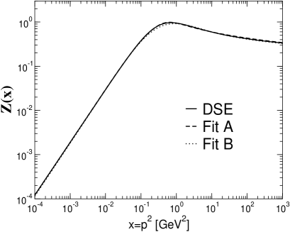
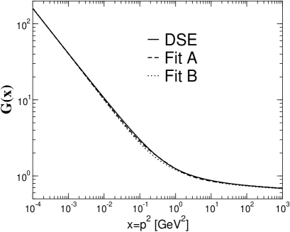
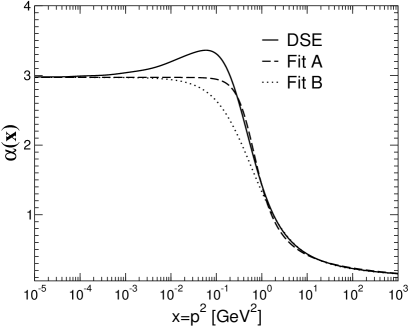
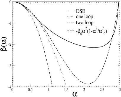
Figure 3.4: Shown are the results for the gluon dressing function $Z$, the ghost dressing function $G$ and the running coupling $\alpha$ using a transverse projector, $\zeta=1$. The two sets of fit functions are given in eqs. (3.57) and (3.58). The $\beta$-function corresponding to our DSE-solution is compared to the one- and two-loop expressions as well as to a polynomial in $\alpha$.

In Fig. 3.4 we show the results for the transverse projector, $\zeta=1$. The gluon and ghost dressing functions behave power-like for low momenta with $\kappa=0.595$ and obey one-loop scaling in the ultraviolet as expected. We found no numerical solution for the second analytical infrared power from subsection 3.3.2, $\kappa\approx 1.3$. We thus conclude, that only the infrared power $\kappa=0.595$ connects to the numerical solution for all momenta. This result will be corroborated in chapter 5. As has been mentioned in the introduction to this chapter first results have been obtained in stochastic quantisation, which is supposed to solve the Gribov problem [18]. The infrared analysis of a bare vertex truncation scheme in stochastic Landau gauge leads to the power $\kappa=0.521$ for the transversal part of the gluon propagator. This is surprisingly close to the value in Faddeev-Popov quantisation and suggests the influence of Gribov copies within the Gribov region to be small.

According to the power solution of the dressing functions the running coupling has a fixed point in the infrared. Furthermore it decreases logarithmically in the perturbative regime above several GeV in accordance with perturbation theory. For intermediate momenta the behaviour of our running coupling induces a node in the $\beta$-function around $(100\mbox{MeV})^{2}$. This, however, corresponds to a double valued $\beta$-function, which is a somewhat strange result not expected from renormalisation group analysis. Therefore we regard it as an artefact of our truncation scheme. Recall from section 3.1 that we have omitted the two-loop diagrams in the gluon equation in all our calculations. Since the two-loop diagrams contain gluon dressing functions only they are subleading in the infrared in the present framework. Furthermore they are subleading in the ultraviolet as can be seen from perturbation theory. Thus the only region where the inclusion of the two-loop diagrams could lead to qualitative corrections of our solutions is the intermediate momentum regime. This is the region where the bump in the coupling appears.

The $\beta$-functions in the bottom right diagram are defined in appendix A.2. Compared to the one- and two-loop $\beta$-functions of perturbation theory the $\beta$-function from our DSE-solution [103] resembles the scaling behaviour of the one-loop result in the ultraviolet, that is for small values of $\alpha$.

The asymptotic behaviour of the solutions can also be seen from the functional form of our fits. We employ two different fit functions [104] for the running coupling $\alpha(x)$:

$$\mbox{Fit A:}\quad\alpha(x) = \frac{\alpha(0)}{\ln[e+a_{1}(x/\Lambda^{2}_{QCD})^{a_{2}}+b_{1}(x/\Lambda^{2}_{QCD})^{b_{2}}]}\,,$$ (3.57)

$$\mbox{Fit B:}\quad\alpha(x) = \frac{1}{a+(x/\Lambda^{2}_{QCD})^{b}}\bigg{[}a\>\alpha(0)+$$ (3.58)

$$\hskip 56.9055pt\left.\frac{4\pi}{\beta_{0}}\left(\frac{1}{\ln(x/\Lambda^{2}_{QCD})}-\frac{1}{x/\Lambda_{QCD}^{2}-1}\right)(x/\Lambda^{2}_{QCD})^{b}\right]\,.\hskip 14.22636pt$$

The value $\alpha(0)=8.915/N_{c}$ is known from the infrared analysis. In both fits the ultraviolet behaviour of the solution fixes the scale, $\Lambda=0.714\,\mbox{GeV}$. Note that we have employed a MOM scheme, and thus $\Lambda_{QCD}$ has to be interpreted as $\Lambda_{MOM}^{N_{f}=0}$, i.e. this scale has the expected magnitude. Fit A employs the four additional parameters: $a_{1}=1.106$, $a_{2}=2.324$, $b_{1}=0.004$, $b_{2}=3.169$. Fit B has only two free parameters: $a=1.020$, $b=1.052$. The dressing functions $Z(x)$ and $G(x)$ are then described by

$$R(x) = \frac{c\,(x/\Lambda^{2}_{QCD})^{\kappa}+d\,(x/\Lambda^{2}_{QCD})^{2\kappa}}{1+c\,(x/\Lambda^{2}_{QCD})^{\kappa}+d\,(x/\Lambda^{2}_{QCD})^{2\kappa}}\,,$$

$$Z(x) = \left(\frac{\alpha(x)}{\alpha(\mu)}\right)^{1+2\delta}R^{2}(x)\,,$$

$$G(x) = \left(\frac{\alpha(x)}{\alpha(\mu)}\right)^{-\delta}R^{-1}(x)\,,$$ (3.59)

where $c,d$ are fitting parameters for the auxiliary function $R(x)$. They are given by $c=1.269$ and $d=2.105$. Recall from subsection 3.3.1 that the anomalous dimension $\gamma$ of the gluon is related to the anomalous dimension $\delta$ of the ghost by $\gamma=-1-2\delta$ and $\delta=-9/44$ for the number of flavours $N_{f}=0$.

     

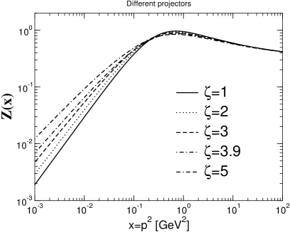
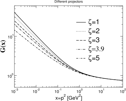
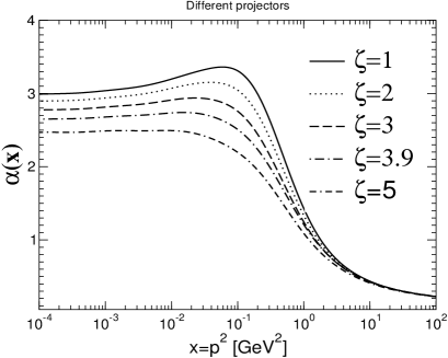
Figure 3.5: Shown are the results for the gluon dressing function, the ghost dressing function and the running coupling, c.f. Fig. 3.4, for different projectors.

Whereas Fit A is better in the region $0.3\,\mbox{GeV}^{2}<x<1\,\mbox{GeV}^{2}$ where $\alpha$ is strongly rising, Fit B is slightly better in the region $1\,\mbox{GeV}^{2}<x<10\,\mbox{GeV}^{2}$, where hadronic $\tau$-decay takes place [105, 106]. As can be seen in Fig. 3.4 both fits works very well and can be used as input for phenomenological calculations in future work.

Our results for different values of the parameter $\zeta$ (c.f. eq. (3.7)) are shown in Fig. 3.5. In accordance with the infrared analysis the power $\kappa$ changes from $\kappa=0.5953$ for $\zeta=1$ to $\kappa=0.4610$ for $\zeta=5$. The perturbative properties of the solutions remain unchanged. The bump in the running coupling gets smaller but does not disappear even for $\zeta=5$. It has already been stated above that the dressing functions would be independent of $\zeta$ in a complete treatment of the gluon equation. As all our solutions are very similar even on a quantitative level we conclude that transversality is lost only to a moderate extent. This is a somewhat surprising result in such a simple truncation scheme as the one at hand.

     

     

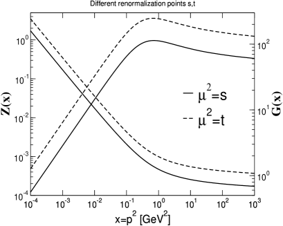
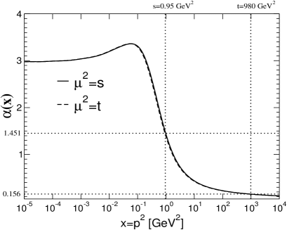
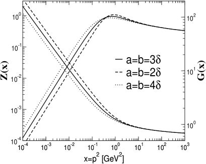
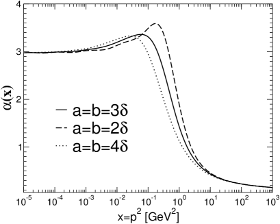
Figure 3.6: Here we display two technical issues. The upper panel shows the ghost and gluon dressing function as well as the running coupling for two different renormalisation points $\mu^{2}=s=0.9\,\mbox{GeV}^{2}$ and $\nu^{2}=t=900\,\mbox{GeV}^{2}$. The independence of the running coupling on the renormalisation point is clearly demonstrated. The lower panel shows the variation of the dressing functions with the parameters $a$ and $b$ from the construction in eq. (3.23). Recall $\delta=-9/44$.

The Brown–Pennington projector, $\zeta=4$, is an exceptional case as can be seen from eqs. (3.47), (3.48). Here the $\kappa$-dependence of the second term cancels and only one solution, $\kappa=1$, can be found (c.f. ref. [82]). We found no numerical solutions for this case. However, within the limit of numerical accuracy, solutions for $\zeta$ slightly different from 4 can be found leading to a value for $\kappa$ slightly different from 1/2. E.g. in Fig. 3.5 the case $\zeta=3.9$ leading to $\kappa=0.5038$ is depicted.

In Fig. 3.6 we discuss two technical issues. First, we demonstrate what happens if we choose two different renormalisation points by specifying two different values for $\alpha(s)=g^{2}/4\pi$. Starting from eqs. (3.18) we can easily see that a change from the renormalisation point $s=\mu^{2}$ to the new value $t$ is performed by

$$G(x,t) = G(x,s)\frac{\tilde{Z}_{3}(s,L)}{\tilde{Z}_{3}(t,L)}\,,$$

$$Z(x,t) = Z(x,s)\frac{{Z}_{3}(s,L)}{{Z}_{3}(t,L)}\,.$$ (3.60)

As the renormalisation constants $\tilde{Z}_{3}$ and $Z_{3}$ are independent of momentum, this results in the mere multiplication of the dressing functions by a constant number. Our numerical results obey exactly this behaviour, as can be seen in the upper right diagram of Fig. 3.6. The running coupling, however, is independent of the renormalisation point, c.f. eq. (3.21), as is clearly demonstrated in the upper right diagram of Fig. 3.6.

In the lower panel of Fig. 3.6 we show what happens when we vary the parameters $a$ and $b$ in our construction of the three-gluon vertex (3.23). Clearly, the qualitative behaviour of the curves does not change. In particular the ultraviolet behaviour of the solutions is independent of the values of $a$ and $b$ in accordance with our analysis in subsection 3.3.1. However, we recognise the rising bump in the running coupling when we lower the absolute values of $a$ and $b$ from $a=b=3\delta$ to $a=b=2\delta$. This corresponds to the equations becoming more and more unstable and no solutions are found for even lower values of $a$ and $b$. The extreme case $a=b=0$, where the gluon loop becomes leading in the infrared, has been investigated in reference [85] with the same negative result: no solutions have been found.

       

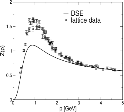
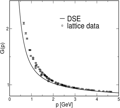
Figure 3.7: Solutions of the Dyson-Schwinger equations compared to recent lattice results for two colours [48, 49].

Finally, we compare our results to recent SU(2) lattice calculations [49, 48]. As has already been stated above the ghost and gluon dressing functions from Dyson-Schwinger equations are independent of the numbers of colours at least to our level of truncation. The only caveat in comparing our results with the lattice ones is the adjustment of the momentum scale. We used the lattice result $\alpha_{SU(2)}(x)=0.68$ at $x=10\,\mbox{GeV}^{2}$ as input, which leads to a slightly different scale than the one used in the case of SU(3). The two graphs in figure (3.7) show that the main qualitative features, the infrared suppression of the gluon dressing function and the divergence of the ghost dressing function are common properties of both, the lattice solutions and the one from Dyson-Schwinger equations. Even the power $\kappa\approx 0.595$ of the gluon dressing function from the DSEs is very close to the one that can be extracted from the lattice fit to be $\kappa\approx 0.5$. The main difference between the two approaches is in the medium energy region around one GeV, where the Dyson-Schwinger solutions suffer from the missing two-loop contributions that are certainly present in lattice Monte-Carlo simulations. The combined evidence of the two methods points strongly towards an infrared vanishing or finite gluon propagator and an infrared singular ghost propagator in Landau gauge.

3.5 Summary

In this chapter we have presented approximate non-perturbative solutions for the gluon and the ghost propagators as well as the running coupling in Landau gauge. We obtained these solutions for the Dyson–Schwinger equations in a truncation scheme working with a bare ghost-gluon vertex and an ansatz for the three-gluon vertex such that we reproduce the correct one-loop scaling of the ghost and gluon dressing functions. We attempt to obtain two-loop scaling by the inclusion of the diagrams that involve four-gluon vertices in future work.

An important improvement to previous treatments has been the explicit numerical calculation of all angular integrals thus overcoming the angular approximations that have been made so far. We could show that for a given projector only one out of two analytical solutions in the infrared can be connected to a numerical solution for finite momenta. For a transversal projector, $\zeta=1$, we found that the gluon propagator is only weakly infrared vanishing, $D_{gluon}(p^{2})\propto(p^{2})^{2\kappa-1}$, $\kappa=0.595\ldots$, and the ghost propagator is highly infrared singular, $D_{ghost}(p^{2})\propto(p^{2})^{-\kappa-1}$. This is in accordance with the Kugo-Ojima confinement criterion and Zwanziger’s horizon condition. The running coupling possesses an infrared fixed point with the value $\alpha(0)\approx 2.97$ (or, for a general number $N_{c}$ of colours, $\alpha(0)\approx 8.92/N_{c}$).

Despite the simplicity of the truncation our solutions agree remarkably well with recent lattice calculations performed for two colours. Due to the finite lattice volume the lattice results cannot, of course, be extended into the far infrared. In this respect our results are complementary to the lattice ones: We do obtain the infrared behaviour analytically. On the other hand, lattice calculations include, at least in principle, all non-perturbative effects whereas we had to rely on truncations. E.g. the deviations for the gluon renormalisation functions at intermediate momenta depicted in Fig. 3.7 might be due to the neglect of the four-gluon vertex function in our calculations.

Chapter 4 Towards general gauges in the DSEs of Yang–Mills theory

In the last chapter we have exploited some properties of Landau gauge that simplify the Dyson-Schwinger equations of the propagators of Yang–Mills theory considerably. The fact that the ghost-gluon vertex is not renormalised in Landau gauge has turned out to be the key for the formulation of our truncation scheme and leads to a useful definition of the non-perturbative running coupling. In other gauges matters are much more complicated and no one has been able to solve the DSEs for general gauges yet. As a first step towards such a solution we present an exploratory study in this chapter. We investigate what happens, when we extend the simple truncation scheme employing bare vertices to the whole family of general gauges which are given by the gauge parameters $\alpha$ and $\lambda$ of the general Lagrangian, eq. (2.11).

Away from the Landau gauge limit no direct connection between the Kugo–Ojima confinement criterion and the infrared behaviour of the ghost dressing function can be seen. This opens the possibility that other degrees of freedom like the longitudinal gluon may take over the infrared dominant role of the ghost dressing function in Landau gauge. As a matter of fact, infrared dominance of longitudinal gluons is seen if stochastic quantisation is used instead of Faddeev–Popov quantisation [18].

This chapter is organised as follows: In the next section we project the ghost and gluon Dyson-Schwinger equations for general gauges onto the respective dressing functions. Then we perform an infrared analysis for the bare vertex truncation of these DSEs. We show that in general ghost-antighost symmetric gauges the genuine two–loop terms (generalised squint and sunset diagram) in the gluon and the ghost DSEs become important in the infrared. This is different from Landau gauge at least in the framework of the bare vertex truncation. In general ghost-antighost symmetric gauges the infrared behaviour of the two-loop terms exclude power-behaved solutions for the gluon and ghost propagators when bare vertices are employed. In section 4.3 we will provide numerical solutions for the DSEs in the Landau gauge limit of the ghost–antighost symmetric case of the Lagrangian and recover the solutions found in the last chapter from a different direction in the two dimensional gauge parameter space [109].

4.1 Projection of the gluon equation

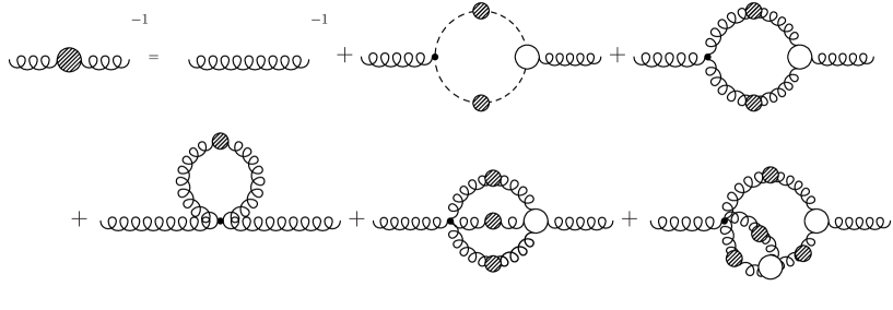
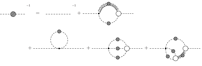
Figure 4.1: The coupled gluon and ghost Dyson–Schwinger equations from a BRS and Anti-BRS symmetric Lagrangian. Each equation contains one-loop diagrams, a tadpole contribution and a sunset and a squint diagram.

In Fig. 4.1 we show again the gluon and ghost Dyson-Schwinger equations for general gauges in diagrammatical notation, c.f. section 2.4. The ghost and gluon equations are remarkably similar, both having tadpole and non-perturbative one-loop and two-loop contributions.

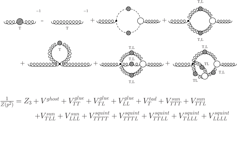
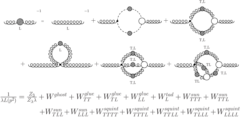
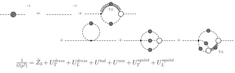
Figure 4.2: Various contributions from the respective diagrams in the transversal (T) and longitudinal (L) gluon equation and the equation for the ghost dressing function.

In order to sort the various contributions of the gluon equation to the inverse of the gluon propagator on the left hand side we project the equation on its longitudinal and transverse parts. It is well known that for linear covariant gauges, i.e. $\alpha=0$, the longitudinal part of the gluon propagator remains undressed [10]. However, away from linear covariant gauges this is not the case as can be seen from the Slavnov-Taylor identity derived in [12]. We then have three dressing functions, $Z,L,G$, in the general case and the propagators are given by

$$D_{\mu\nu}(p) = \left[D_{\mu\nu}(p)\right]_{T}+\left[D_{\mu\nu}(p)\right]_{L}$$ (4.1)

$$= \left(\delta_{\mu\nu}-\frac{p_{\mu}p_{\nu}}{p^{2}}\right)\frac{Z(p^{2})}{p^{2}}+\lambda L(p^{2})\frac{p_{\mu}p_{\nu}}{p^{4}}\,,$$

$$D_{G}(p) = -\frac{G(p)}{p^{2}}\,.$$ (4.2)

The transversal and longitudinal gluon dressing functions $Z(p^{2})$ and $L(p^{2})$ can be extracted by contracting the gluon equation with the transversal and longitudinal projector respectively. The results are given graphically in Fig. 4.2, where we also specify our notation for the different contributions being analysed in the next section. Contributions in the transversal part of the gluon equation are denoted by the symbol $V$, contributions in the longitudinal part by $W$ and the ones in the ghost equation by $U$. The subscripts $T$ and $L$ indicate the respective parts of the gluon propagator running around in the loops of the diagrams and abbreviations for the names of the diagrams are used. For example the symbol $W^{sun}_{LLT}$ denotes a contribution from the sunset diagram to the longitudinal gluon equation with two longitudinal and one transverse part of the gluon propagator running in the loop. To isolate the dressing functions the left hand sides of the equations have already been divided by factors of $3p^{2}$ and $p^{2}$, respectively.

4.2 Infrared analysis with bare vertices for arbitrary gauge parameters

We are now ready to determine the behaviour of the two-point functions at small momenta $p^{2}$, in a way very similar to our analysis in the last chapter for Landau gauge. In section 3.2.1 we discussed the central observation in Landau gauge, that there is no qualitative difference of the solutions found with bare vertices or with vertices dressed by the use of Slavnov-Taylor identities. This has been shown recently for a range of possible vertex dressings in a truncation scheme without any angular approximations [70]. The reason for this somewhat surprising result has been attributed to the non-renormalisation of the ghost-gluon vertex in Landau gauge, i.e. $\tilde{Z}_{1}=1$. It seems as if the violation of gauge invariance using a bare vertex is not that severe in Landau gauge such that the resulting equations still provide meaningful results. In the following we will explore to what extent such a simple truncation idea is applicable in other gauges.

Our power law ansatz for the dressing functions is

$$G(x)=Bx^{\beta},\>\>\>\>Z(x)=Ax^{\sigma},\>\>\>\>L(x)=Cx^{\rho},$$ (4.3)

where $x=p^{2}$ has been used. Together with the expressions for the bare vertices given in appendix A.3 we plug the power laws into the ghost and the gluon equation. The formulae for the various integrals are given in appendix C.2. The straightforward but tedious algebra is done with the help of the algebraic manipulation program FORM [96]. In section 3.3.2 we have argued that the renormalisation constants $Z_{3}$ and $\tilde{Z}_{3}$ can be dropped in the infrared analysis. Furthermore the tadpoles just give constant contributions to the respective propagators which vanish in the process of renormalisation. Thus we can safely omit them in the present investigation.

For general gauges, $\alpha\neq 0$ and $\lambda\neq 0$, we obtain the following structure:

$$B^{-1}x^{-\beta} = x^{\sigma+\beta}(U^{\prime})^{dress}_{T}+x^{\rho+\beta}(U^{\prime})^{dress}_{L}+x^{3\beta}(U^{\prime})^{sun}$$ (4.4)

$$+x^{\sigma+3\beta}(U^{\prime})^{squint}_{T}+x^{\rho+3\beta}(U^{\prime})^{squint}_{L}\,,$$

$$A^{-1}x^{-\sigma} = x^{2\beta}(V^{\prime})^{ghost}+x^{2\sigma}(V^{\prime})^{glue}_{TT}+x^{\sigma+\rho}(V^{\prime})^{glue}_{TL}+x^{2\rho}(V^{\prime})^{glue}_{LL}$$ (4.5)

$$+x^{3\sigma}(V^{\prime})^{sun}_{TTT}+x^{2\sigma+\rho}(V^{\prime})^{sun}_{TTL}+x^{\sigma+2\rho}(V^{\prime})^{sun}_{TLL}+x^{3\rho}(V^{\prime})^{sun}_{LLL}$$

$$+x^{4\sigma}(V^{\prime})^{squint}_{TTTT}+x^{3\sigma+\rho}(V^{\prime})^{squint}_{TTTL}+x^{2\sigma+2\rho}(V^{\prime})^{squint}_{TTLL}$$

$$+x^{\sigma+3\rho}(V^{\prime})^{squint}_{TLLL}+x^{4\rho}(V^{\prime})^{squint}_{LLLL}\,,$$

$$\left(C\lambda\right)^{-1}x^{-\rho} = +x^{2\beta}(W^{\prime})^{ghost}+x^{2\sigma}(W^{\prime})^{glue}_{TT}+x^{\sigma+\rho}(W^{\prime})^{glue}_{TL}$$ (4.6)

$$+x^{3\sigma}(W^{\prime})^{sun}_{TTT}+x^{2\sigma+\rho}(W^{\prime})^{sun}_{TTL}+x^{\sigma+2\rho}(W^{\prime})^{sun}_{TLL}+x^{3\rho}(W^{\prime})^{sun}_{LLL}$$

$$+x^{4\sigma}(W^{\prime})^{squint}_{TTTT}+x^{3\sigma+\rho}(W^{\prime})^{squint}_{TTTL}+x^{2\sigma+2\rho}(W^{\prime})^{squint}_{TTLL}$$

$$+x^{\sigma+3\rho}(W^{\prime})^{squint}_{TLLL}\,.$$

Here the primed quantities $U^{\prime}$, $V^{\prime}$ and $W^{\prime}$ are momentum independent functions of the exponents $\beta$, $\sigma$ and $\rho$. The corresponding momentum dependent quantities $U$, $V$ and $W$ have been introduced in Fig. 4.2. The pattern of the equation is such that each primed factor on the right hand side is accompanied by the squared momentum $x$ to the power of the dressing function content of the respective diagram. In appendix C.3 we demonstrate how such a pattern emerges for the example of the sunset diagram in the ghost equation, $(U)^{sun}$. Note that the contributions $(W^{\prime})^{glue}_{LL}$ and $(W^{\prime})^{squint}_{LLLL}$ are zero and therefore missing in the longitudinal gluon equation (4.6) as momentum conservation cannot hold with three longitudinal gluons in the three gluon vertex.

For the following argument we focus on one particular contribution on each right hand side of the equations, keeping in mind that all other contributions have no explicit minus sign in the exponents:

$$B^{-1}x^{-\beta} = x^{3\beta}(U^{\prime})^{sun}+\ldots\,,$$ (4.7)

$$A^{-1}x^{-\sigma} = x^{4\sigma}(V^{\prime})^{squint}_{TTTT}+\ldots\,,$$ (4.8)

$$\left(C\lambda\right)^{-1}x^{-\rho} = x^{3\rho}(W^{\prime})^{sun}_{LLL}+\ldots\,.$$ (4.9)

In general the coefficients $(U^{\prime})^{sun}$, $(V^{\prime})^{squint}_{TTTT}$ and $(W^{\prime})^{sun}_{LLL}$ are nonzero and explicitly given in appendix C.3. First, it is easy to see from equations (4.7), (4.8) and (4.9) that neither $\beta$ nor $\sigma$ nor $\rho$ can be negative. If one of these powers would be negative the limit $x\rightarrow 0$ would lead to a vanishing left hand side of the respective equation whereas the right hand side is singular in this limit. This is a contradiction as the power on the left hand side of the equation should match the leading power on the right hand side. Second, if one of the exponents $\beta$, $\sigma$ or $\rho$ would be positive, then the diverging left hand side of the respective equation would require a diverging term on the right hand side as well. However, we already saw that $\beta$, $\sigma$ or $\rho$ cannot be negative and therefore we have no diverging term on the right hand side of the equations. Thus none of the exponents $\beta$, $\sigma$ and $\rho$ can be positive. The remaining possibility is $\beta=\sigma=\rho=0$, but then we have logarithms on the right hand side of the equation which do not match the constant on the left hand side. Thus we arrive at the conclusion that there is no power solution for general gauges when bare vertices are used.

There are two limits for the gauge parameters $\alpha$ and $\lambda$ in which the situation changes. The first one is $\alpha=0$, that are ordinary linear covariant gauges. Due to the corresponding Slavnov-Taylor identity the longitudinal part of the gluon propagator remains undressed, $L(p^{2})=1$ [10]. The longitudinal gluon equation becomes trivial as the Slavnov-Taylor identity forces all nontrivial contributions on the right hand side to cancel each other. In the ghost equation the squint as well as the sunset diagram disappear, i.e. $(U^{\prime})^{sun}=(U^{\prime})^{squint}=0$. The term of the dressing loop which contains the longitudinal part of the gluon propagator, $(U^{\prime})^{dress}_{L}$, vanishes as well, c.f. appendix C.3. We are left with the contribution $U^{dress}_{T}\sim x^{(\beta+\sigma)}$, similar to Landau gauge. This is the reason why we escape the argument given below eq. (4.9). The explicit expression for the ghost equation is given by

$$B^{-1}x^{-\beta} = x^{(\beta+\sigma)}\frac{g^{2}N_{c}\tilde{Z}_{1}AB}{16\pi^{2}}\,\frac{-3}{2\,(\beta+\sigma)\,(-1+\beta+\sigma)}\times$$ (4.10)

$$\hskip 142.26378pt\times\frac{\Gamma(2-\beta-\sigma)\,\Gamma(1+\sigma)\,\Gamma(2+\beta)}{\Gamma(3+\beta+\sigma)\,\Gamma(2-\sigma)\,\Gamma(1-\beta)}.$$

which can be compared with the Landau gauge expression, eq. (3.42). Matching left and right hand sides we conclude that the Landau gauge result

$$\sigma=-2\beta$$ (4.11)

is valid for all linear covariant gauges when bare vertices are used.

Compared to general gauges the gluon equation does not change in structure when $\alpha=0$. Therefore we still have $\sigma>0$, according to the argument given below eq. (4.9). The identity (4.11) thus requires $\beta<0$ and we have a divergent ghost and a vanishing gluon dressing function in the infrared similar to Landau gauge. With bare vertices this implies that the ghost loop is the dominant contribution in the gluon equation for small momenta. Since the ghost loop is independent of the gauge parameter $\lambda$, our Landau gauge results of section 3.3.2 for the exponent $\kappa=-\beta=\sigma/2$ are valid for all linear covariant gauges. However, a word of caution is in order. In Landau gauge there are indications [66, 68] that the general result (4.11) does not change when the vertices are dressed. This has been confirmed recently for a range of possible vertex dressings [70]. It is a completely open question whether this is the same for $\lambda\neq 0$.

Having addressed the case of linear covariant gauges with $\alpha=0$ we now turn to the other interesting limit, i.e. $\lambda=0$ while $\alpha\neq 0$. It is easy to see that the $\alpha$-dependence of the Lagrangian (2.11) can be eliminated in this case by partial integration using the constraint $\partial_{\mu}A_{\mu}=0$. However, on the level of the DSEs with bare vertices there remain spurious $\alpha$-dependent terms on the right hand side of the gluon equation. In the next section we will investigate the dependence of the Landau gauge solution on the gauge parameter $\alpha$ if these spurious terms are present.

4.3 Solutions in Landau gauge

To assess the influence of the spurious $\alpha$-terms in Landau gauge we use the truncation scheme of section 3.3. Again we employ the general tensor

$${\mathcal{P}}^{(\zeta)}_{\mu\nu}(p)=\delta_{\mu\nu}-\zeta\,\frac{p_{\mu}p_{\nu}}{p^{2}}$$ (4.12)

to contract the Lorenz indices in the gluon equation. By varying the parameter $\zeta$ we are able to test additionally for spurious longitudinal terms. For $\lambda=0$ and general values of the gauge parameter $\alpha$ the coupled set of equations for the ghost and gluon dressing functions are (c.f. eqs. (3.24), (3.25), (3.26), (3.32), where $\alpha=0$)

$$\frac{1}{G(x)} = Z_{3}-g^{2}N_{c}\int\frac{d^{4}q}{(2\pi)^{4}}\frac{K(x,y,z)}{xy}G(y)Z(z)\;,$$ (4.13)

$$\frac{1}{Z(x)} = \tilde{Z}_{3}+g^{2}\frac{N_{c}}{3}\int\frac{d^{4}q}{(2\pi)^{4}}\frac{M(x,y,z)}{xy}G(y)G(z)$$ (4.14)

$$\hskip 17.07182pt+g^{2}\frac{N_{c}}{3}\int\frac{d^{4}q}{(2\pi)^{4}}\frac{Q(x,y,z)}{xy}\frac{G(y)^{(1-a/\delta-2a)}}{Z(y)^{a}}\frac{G(z)^{(1-b/\delta-2b)}}{Z(z)^{b}}\;.$$

The kernels ordered with respect to powers of $z:=p^{2}=(k-q)^{2}$ have the form:

$$K(x,y,z) = \frac{1}{z^{2}}\left(-\frac{(x-y)^{2}}{4}\right)+\frac{1}{z}\left(\frac{x+y}{2}\right)-\frac{1}{4}\,,$$

$$M(x,y,z) = \frac{1}{z}\left(\frac{(\zeta-1)\alpha^{2}-(\zeta-1)2\alpha+\zeta-2}{4}x+\frac{y}{2}-\frac{\zeta}{4}\frac{y^{2}}{x}\right)+\frac{1}{2}+\frac{\zeta}{2}\frac{y}{x}-\frac{\zeta}{4}\frac{z}{x}\,,\hskip 28.45274pt$$

$$Q(x,y,z) = \frac{1}{z^{2}}\left(\frac{1}{8}\frac{x^{3}}{y}+x^{2}-\frac{19-\zeta}{8}xy+\frac{5-\zeta}{4}y^{2}+\frac{\zeta}{8}\frac{y^{3}}{x}\right)$$ (4.15)

$$+\frac{1}{z}\left(\frac{x^{2}}{y}-\frac{15+\zeta}{4}x-\frac{17-\zeta}{4}y+\zeta\frac{y^{2}}{x}\right)$$

$$-\left(\frac{19-\zeta}{8}\frac{x}{y}+\frac{17-\zeta}{4}+\frac{9\zeta}{4}\frac{y}{x}\right)$$

$$+z\left(\frac{\zeta}{x}+\frac{5-\zeta}{4y}\right)+z^{2}\frac{\zeta}{8xy}+\frac{5}{4}(4-\zeta)\,.$$

      

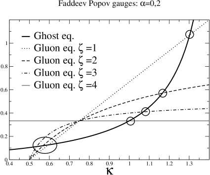
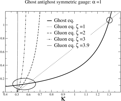
Figure 4.3: Here the graphical solution to equation (4.17) is shown. The thick line represents the left hand side of equation (4.17), whereas the other curves depict the right hand side for different values of the parameters $\zeta$. The left figure shows results for $\alpha=0$ and $\alpha=2$, whereas in the figure on the right we have $\alpha=1$. The ellipses mark the bulk of solutions between $\kappa=0.5$ and $\kappa=0.6$, whereas the circles show spurious solutions with $\kappa\geq 1$.

First we accomplish the infrared analysis. With $\kappa=-\beta=\sigma/2$ we employ the ansatz

$$Z(x)=Ax^{2\kappa}\,,\>\>\>\>\>\>\>G(x)=Bx^{-\kappa}$$ (4.16)

in the equations (4.13) and (4.14). After integration we match coefficients of equal powers on both sides of the equations and obtain

$$\frac{1}{18}\frac{(2+\kappa)(1+\kappa)}{(3-2\kappa)}$$

$$=\frac{(4\kappa-2)\,(-1+\kappa)}{(\zeta-1)\left[4\,\kappa^{2}\,(\alpha^{2}-2\,\alpha+1)+8\,\kappa\,\alpha\,(2-\alpha)+3\,\alpha\,(\alpha-2)\right]+\kappa\,(10-7\,\zeta)-6+3\,\zeta}\;.$$

(4.17)

The values of $\kappa$ for different tensors $\mathcal{P}^{(\zeta)}$ can be read off Fig. 4.3. The curve given by the fully drawn line represents the term on the left hand side of eq. (4.17), whereas the other lines depict the right hand side for several values of the parameter $\zeta$. The solutions between $\kappa=0.5$ and $\kappa=0.6$ remain nearly unchanged when $\alpha$ is varied, whereas the solutions for $\kappa>1$ are only present when $\alpha=0,2$. In the last chapter we found that only the solutions $\kappa\approx 0.5$ connect to numerical results for finite momenta. It is satisfactory to observe that by varying the gauge parameter $\alpha$ such solutions can be identified as spurious already on the level of the infrared analysis.

     

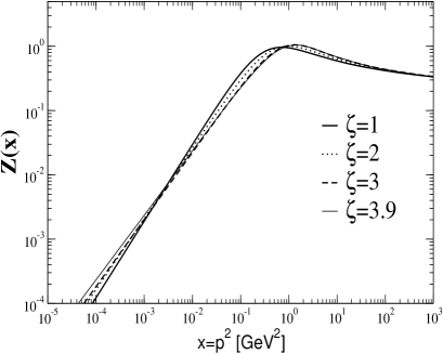
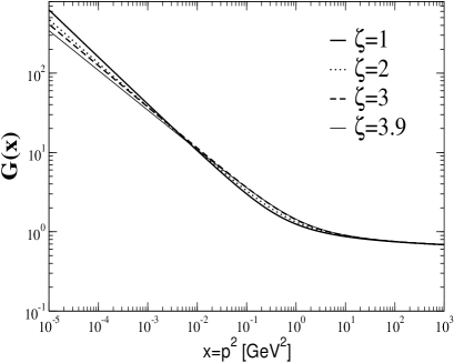
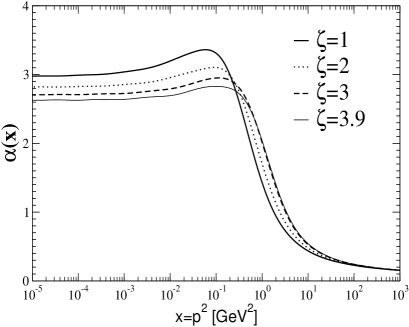
Figure 4.4: Here we display the gluon dressing function, $Z(x)$, the ghost dressing function, $G(x)$ and the running coupling $\alpha(x)$ in the truncation scheme of chapter 3 for the gauge parameters $\alpha=1$ and $\lambda=0$ and different tensors $\mathcal{P}^{(\zeta)}$ employed in the gluon equation.

We now explore the impact of the spurious $\alpha$ term on the behaviour of the solutions for all momenta $x$. We solved the equations (4.13) and (4.14) numerically using the technique described in appendix C.4. Compared to the usual Landau gauge, $\alpha=0$, we obtain the greatest deviations for the ghost-antighost symmetric case, $\alpha=1$. The results can be seen in Fig. (4.4). As the dependence of the kernel of the ghost loop on $\alpha$ vanishes in the case of the transverse projector, $\zeta=1$, this solution is identical with the one displayed in Fig. 3.4 in subsection 3.4.2. For the other cases the power $\kappa$ changes from $0.5953$ for $\zeta=1$ to $0.5020$ for $\zeta=3.9$ in accordance with the infrared analysis. The ultraviolet properties of the solutions are slightly disturbed compared to the case $\alpha=0,2$. An analytical ultraviolet analysis similar to the one in subsection 3.3.1 reveals that the $\alpha$-term in the ghost loop induces a spurious dependence of the anomalous dimensions on the parameter $\zeta$:

$$\gamma = \frac{-26-(\zeta-1)\,\alpha\,(2-\alpha)}{44+(\zeta-1)\,\alpha\,(2-\alpha)}$$

$$\delta = \frac{-9}{44+(\zeta-1)\,\alpha\,(2-\alpha)}$$ (4.18)

For general $\alpha$ only the transverse projector removes the alpha-term in the ghost equation and leads to the correct one loop scaling of the equations, that is $\delta=-9/44$ for the ghost and $\gamma=-13/22$ for the gluon dressing function for an arbitrary number of colours and zero flavours.

4.4 Summary

We have studied the infrared behaviour of the ghost and gluon propagators in covariant ghost-antighost symmetric gauges. We derived the corresponding Dyson–Schwinger equations for these propagators including the ones of linear covariant gauges as the limit of a vanishing gauge parameter. Note that ghost-antighost symmetric gauges are particularly interesting as they allow an interpretation of the antighost field being the antiparticle of the ghost which includes also the possibility of ghost-antighost condensates. Due to the emergence of a four-ghost interaction term in the Lagrangian for general values of the gauge parameters the Dyson–Schwinger equation of the ghost propagator displays a rich structure very similar to the one of the gluon equation. On the other hand, in the gluon equation we obtain the same structure as in linear covariant gauges apart from the fact that the gluon propagator acquires a nontrivial longitudinal part which appears in turn in all diagrams. The gluon and ghost equations depend therefore on three independent dressing functions, one for the ghost, one for the transversal part of the gluon propagator and one for the longitudinal one.

We then employed a truncation scheme for the Dyson–Schwinger equations that uses bare vertices in place of the dressed ones. The success of this particular truncation scheme in Landau gauge has been attributed to the non-renormalisation of the ghost-gluon vertex, i.e. $\widetilde{Z}_{1}=1$. We addressed the infrared behaviour of the ghost and gluon propagators for general gauges by employing power law ansätze for the respective dressing functions. We then have been able to evaluate the infrared behaviour of the gluon and ghost equations analytically.

For all linear covariant gauges we find a similar result as compared to the one in Landau gauge: An infrared suppressed gluon propagator and an infrared enhanced ghost. Whereas in Landau gauge there are indications that this generic result is not changed when the vertices are dressed [70], it remains an open question whether this is the case in linear covariant gauges in general. Away from linear covariant gauges, i.e. in the general case $\alpha\not=0$ and $\lambda\not=0$, we do not find power solutions for the dressing functions. Again, this might be altered significantly by appropriate vertex dressings. Nevertheless, it remains to be emphasised that therefore also the occurrence of a ghost-antighost vacuum condensate is excluded in this specific truncation scheme within this class of gauges.

A special case among all gauges considered here is Landau gauge. In the limit $\lambda=0$ the general Lagrangian (2.11) becomes independent of the second gauge parameter $\alpha$, thus Landau gauge is also a special case of ghost-antighost symmetric gauges. Although the Lagrangian of the theory is independent of the gauge parameter $\alpha$, our simple truncation scheme breaks this invariance and spurious $\alpha$-dependent terms arise in the ghost loop of the gluon Dyson–Schwinger equation. Examining the case $\alpha=1$ we showed that the influence of these spurious terms is very small. We determined solutions for the ghost and gluon dressing functions both analytically in the infrared and numerically for finite momenta and found solutions close to the ones of chapter 3. We thus recovered the results of Landau gauge from a different direction in the two dimensional space of gauge parameters.

Chapter 5 Landau gauge Yang-Mills theory on a four-torus

There are a number of central aims connected to the investigation of the Dyson–Schwinger equations on a four-torus. The first one is purely technical: This allows to study finite volume effects also in the Dyson–Schwinger approach. Monte-Carlo simulations on a lattice necessarily have to be done in a finite volume. Therefore in the latter kind of approach infrared properties are only accessible by extrapolations to an infinite volume. However, the avaliable data are gained on volumes which differ at best by one order of magnitude due to limitations in computer time. We will see in the present Dyson–Schwinger approach that available volumes cover several orders of magnitude. And more importantly, one can compare to the results obtained in an infinite volume for several truncation schemes.

The second issue is the connection of analytical solutions obtained in the infrared limit of the (truncated) Dyson–Schwinger equations to the numerical solution obtained for finite momenta up to the ultraviolet. In chapter 3 we have seen that not every analytical solution in the infrared connects to such a numerical solution. By imposing different infrared boundary conditions on our numerical equations we could check, whether a given infrared solution is connected to a numerical solution for finite momenta and which is not. In this chapter we will verify this procedure by an even stronger selection process: Due to the finite volume there is no input in the infrared and our numerical solutions on a four-torus choose their infrared behaviour by themselves. We will see, that the same infrared solutions are chosen than in the continuum.

The third issue is that once we know how to treat Dyson–Schwinger equations on a torus several interesting possibilities for further investigations open up. Choosing an asymmetric four-torus might allow the introduction of a non-vanishing temperature [110] in a relatively simple way. Furthermore there is the possibility of topological obstructions on a compact manifold. It is well known e.g. that a four-torus allows for a non-vanishing Pontryagin index [111]. Moreover one could think of choosing twisted boundary conditions [112, 113].

This chapter is organised as follows: In the first section we summarise the truncation schemes of [66, 79] and [67] in more detail. They serve as simple test cases to check the feasibility of Dyson-Schwinger calculations on a compact manifold. In the second section we set up the Dyson-Schwinger equations on a four-torus and discuss their numerical treatment. In the last section of this chapter we display our numerical results for three different truncation schemes: the two summarised in the next section and the new truncation scheme introduced already in chapter 3. We discuss the finite volume effects of our solutions [83] and perform a preliminary infinite volume extrapolation.

5.1 A summary of two truncation schemes employing angular approximations

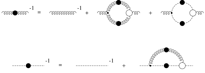
Figure 5.1: Diagrammatic representation of the truncated gluon and ghost Dyson–Schwinger equations according to the truncation schemes studied in this chapter.

One central aim of the present investigation is to answer the question, how the ghost and gluon propagators are affected by finite volume effects on a torus. We will therefore compare solutions of the continuum DSEs with results obtained from the respective equations on the torus. To be able to distinguish genuine finite volume effects from effects arising only in certain truncation schemes we will study not only the scheme defined in chapter 3 but also the two previous truncation schemes of refs. [66, 79, 67] on a torus. All three truncation schemes take into account the loops displayed in Fig. 5.1. However, contrary to our calculation in chapter 3 the two previous schemes employ an angular approximation in the loop integrals, c.f. the discussion in section 3.2. This angular approximation turned out to be good in the ultraviolet but less trustable for small momenta. We therefore consider the system given in chapter 3 to capture more of the essential physics of the coupled ghost and gluon system. Nevertheless when it comes to a study of finite volume effects it seems helpful to employ all three truncation systems.

To proceed we will summarise the truncation schemes of refs. [66, 79, 67] in the next two subsections. The main difference between these two truncation schemes is the treatment of the three-point functions. Whereas in ref. [66] approximate Slavnov–Taylor identities have been employed to construct an ansatz for the vertices, in ref. [67] bare three-point functions have been used. Amazingly, though, both schemes provide results with identical qualitative infrared behaviour: the gluon propagator vanishes in the infrared, the ghost propagator is highly singular there, and the strong running coupling has an infrared fixed point.

5.1.1 The dressed vertex truncation including the gluon loop

In section 3.2 we already discussed the full Slavnov-Taylor identity for the ghost-gluon vertex, c.f. eq. (3.9). Neglecting the irreducible four-ghost term this identity and the corresponding one for the three-gluon vertex are solved by the vertices [66]

$$\Gamma_{\mu}(p,q) = iq_{\mu}\left(\frac{G(k^{2})}{G(q^{2})}+\frac{G(k^{2})}{G(p^{2})}-1\right)\,,$$ (5.1)

$$\Gamma_{\mu\nu\rho}(p,q,k) = A_{+}(p^{2},q^{2},k^{2})\,\delta_{\mu\nu}(p-q)_{\rho}+A_{-}(p^{2},q^{2},k^{2})\,\delta_{\mu\nu}(p+q)_{\rho}$$ (5.2)

$$+2\frac{A_{-}(p^{2},q^{2},k^{2})}{p^{2}-q^{2}}(\delta_{\mu\nu}\,p.q-p_{\nu}q_{\mu})(p-q)_{\rho}\,\,+\,\,\mbox{cyclic permut.}\,\,,$$

with

$$A_{\pm}(p^{2},q^{2},k^{2})=\frac{G(k^{2})}{2}\left(\frac{G(q^{2})}{G(p^{2})Z(p^{2})}\pm\frac{G(p^{2})}{G(q^{2})Z(q^{2})}\right)\,.$$ (5.3)

Here $k^{2}=(p-q)^{2}$ denotes the gluon momentum in the ghost-gluon vertex $\Gamma_{\mu}$. The three-gluon vertex $\Gamma_{\mu\nu\rho}$ is completely symmetric in the three momenta.

The Lorenz indices in the gluon equation are contracted with the Brown-Pennington projector, eq. (3.6). In order to obtain the correct scaling behaviour of the gluon loop in the ultraviolet the substitution

$$Z_{1}\>\>\longrightarrow\>\>{\mathcal{Z}}_{1}(q^{2})=\frac{G(q^{2})^{(-2-6\delta)}}{Z(q^{2})^{(1+3\delta)}}\,,$$ (5.4)

for the vertex renormalisation constant $Z_{1}$ has been introduced. Here the squared momentum $q^{2}$ denotes the momentum integrated over in the gluon loop. Recall the anomalous dimension of the ghost, $\delta=-9/44$, for an arbitrary number of colours and zero flavours.

Furthermore in ref. [66] the so called modified angular approximations

$$Z(z),G(z)\simeq Z(x),G(x) \longrightarrow Z(y),G(y)\quad\mbox{if}\quad x\leq y\,,$$

$$Z(z),G(z) \longrightarrow Z(x),G(x)\quad\mbox{if}\quad x>y\,,$$ (5.5)

have been employed. The approximation in the first equation is designed to eliminate a spurious term stemming from the vertex construction (c.f. the discussion in subsection 3.2.1). Since the presence of this spurious term causes a fatal inconsistency in the ghost equation [67], this modified angular approximation is a central ingredient in this truncation scheme.

Collecting all this together one arrives at the equations

$$\frac{1}{G(x)} = \tilde{Z}_{3}-N_{c}\frac{g^{2}}{(2\pi)^{4}}\left\{\int_{0}^{x}d^{4}q\>\frac{{\sin}^{2}\Theta}{z^{2}}\>G(x)\>Z(x)+\int_{x}^{L}d^{4}q\>\frac{{\sin}^{2}\Theta}{z^{2}}\>G(y)\>Z(y)\right\},\hskip 28.45274pt{}$$ (5.6)

$$\frac{1}{Z(x)} = Z_{3}+\frac{N_{c}}{6}\frac{g^{2}}{(2\pi)^{4}}\int_{0}^{L}d^{4}q\>\frac{N(x,y,z)}{xyz}\>Z(y)^{-3\delta}\>G(y)^{(-1-6\delta)}$$ (5.7)

$$+\frac{N_{c}}{3}\frac{g^{2}}{(2\pi)^{4}}\left\{\int_{0}^{x}d^{4}q\>\left(\frac{1-4\cos^{2}\Theta}{xz}\>G^{2}(x)+\frac{3p\cdot q}{xyz}\>G(x)\>G(y)\right)\right.$$

$$\hskip 139.41832pt+\left.\int_{x}^{L}d^{4}q\>\left(\frac{1-4\cos^{2}\Theta}{xz}+\frac{3p\cdot q}{xyz}\right)G^{2}(y)\right\}\,,$$

for the ghost and gluon dressing function [66]. For ease of notation we have used the abbreviations $x:=p^{2}$, $y:=q^{2}$ and $z:=(p-q)^{2}$ for the squared momenta. Furthermore an $O(4)$–invariant momentum cutoff $L=\Lambda^{2}$ has been introduced. The integral kernel $N(x,y,z)$ is given by

$$N(x,y,z) = \frac{1}{4xyz}\left(4z^{4}+32z^{3}y+2z^{3}x-26z^{2}xy-15z^{2}x^{2}-72z^{2}y^{2}+32zy^{3}\right.$$ (5.8)

$$\left.-38zyx^{2}+8x^{3}z-26zy^{2}x+2y^{3}x+x^{4}+4y^{4}-15y^{2}x^{2}+8x^{3}y\right)\,,\hskip 14.22636pt$$

and the angle $\Theta$ is defined by $z=(q-p)^{2}=x+y-2\sqrt{xy}\cos\Theta$. The equations (5.6) and (5.7) will be implemented on a four-torus in section 5.2.

In the continuum one is now able to carry out the angular integrals analytically and solve the equations along the lines described in ref. [66, 91, 114]. In the infrared the solutions $Z(x)$ and $G(x)$ behave power-like,

$$Z(x)=Ax^{2\kappa},\quad G(x)=Bx^{-\kappa},$$ (5.9)

with uniquely related coefficients $A$ and $B$. In this truncation scheme one obtains $\kappa\approx 0.92$. For three colours the running coupling approaches the fixed point $\alpha(0)\approx 9.5$ in the infrared [66, 79].

The dressed vertex truncation scheme of Hauck, Smekal and Alkofer has been the first one to include both the gluon and the ghost dressing function. Compared to the old truncation of Mandelstam [95], which completely neglects the effects of ghosts, this has been a major improvement. Whereas the Mandelstam equation is solved by a gluon dressing function which diverges in the infrared, the inclusion of ghosts leads to the qualitatively different picture of an infrared vanishing gluon dressing function and a diverging ghost. This new picture, contradicting the old idea of infrared slavery, has been corroborated since in other Dyson-Schwinger studies [67, 68, 62, 70] as well as lattice calculations [65, 71, 72, 73, 74, 75, 76].

One of the original strengths of the dressed vertex truncation scheme, namely the construction of the vertices as solutions of approximate Slavnov-Taylor identities, is considered as a weakness in the meantime. The so constructed vertex ansätze have been shown to be not in accordance with perturbation theory [92, 93] and, much worse, lead to inconsistent equations when no angular approximations are employed. This is the central reason why we did not use the vertices (5.1) and (5.2) in our truncation scheme of chapter 3.

5.1.2 The bare vertex ’ghost-loop only’ truncation

In ref. [67] also a bare ghost-gluon vertex has been used. In section 3.2 we have discussed at length why the bare vertex is capable of providing reliable results even in the infrared region of momentum, where one would expect effects from non-perturbative vertex dressing to be most pronounced. In the gluon loop the authors of [67] use a bare three-gluon vertex without modifying the vertex renormalisation constant $Z_{1}$. As this construction neither restores a correct perturbative limit of the equations (c.f. our discussion in section 3.3) nor changes the infrared behaviour of the solutions, the authors themselves omit the gluon loop in the main part of their investigation.

Substituting the tree-level ghost-gluon vertex for the dressed one and neglecting the gluon loop the coupled system of equations (5.7) reads

$$\frac{1}{G(x)} = \tilde{Z}_{3}-g^{2}N_{c}\int\frac{d^{4}q}{(2\pi)^{4}}\frac{K(x,y,z)}{xy}G(y)Z(z)\;,$$ (5.10)

$$\frac{1}{Z(x)} = {Z}_{3}+g^{2}\frac{N_{c}}{3}\int\frac{d^{4}q}{(2\pi)^{4}}\frac{M(x,y,z)}{xy}G(y)G(z)\,.$$ (5.11)

Again we used the abbreviations $x:=p^{2}$, $y:=q^{2}$, $z:=(q-p)^{2}$, $s:=\mu^{2}$ and $L:=\Lambda^{2}$. The kernels $K$ and $M$ are already given in eqs. (3.26). The ghost equation (5.10) and the ghost loop (5.11) are identical to the ones of our truncation in section 3.3, provided the projection parameter $\zeta$ is set to the special case $\zeta=4$ (c.f. eqs. (3.7), (3.24), (3.25)). As the ghost loop is the leading part of the gluon equation, both schemes share the same infrared behaviour for $\zeta=4$. Indeed, we have found the infrared solution $\kappa=1$ in subsection 3.3.2 in accordance with the infrared analysis in [82], where no angular approximation has been employed. However, we were not able to find a numerical solution for finite momenta connecting to $\kappa=1$ in the infrared as has been detailed in section 3.4.2.

Thus, similar to the truncation scheme summarised in the last subsection, one only gets numerical solutions for finite momenta once an angular approximation has been employed. The authors of [67] use the so called ymax-approximation

$$Z(z),G(z)\longrightarrow Z({\rm max}(x,y)),G({\rm max}(x,y)).$$ (5.12)

Upon angular integration the eqs. (5.10), (5.11) are then simplified to

$$\frac{1}{G(x)} = \widetilde{Z}_{3}(s,L)-\frac{9}{4}\frac{g^{2}N_{c}}{48\pi^{2}}\left(Z(x)\int_{0}^{x}\frac{dy}{x}\frac{y}{x}G(y)+\int_{x}^{L}\frac{dy}{y}Z(y)G(y)\right),$$ (5.13)

$$\frac{1}{Z(x)} = Z_{3}(s,L)+\frac{g^{2}N_{c}}{48\pi^{2}}\left(G(x)\int_{0}^{x}\frac{dy}{x}\left(-\frac{y^{2}}{x^{2}}+\frac{3y}{2x}\right)G(y)+\int_{x}^{L}\frac{dy}{2y}G^{2}(y)\right).$$ (5.14)

In the infrared the solutions of eqs. (5.13,5.14) behave power-like, c.f. eq. (5.9), with $\kappa\approx 0.77$. The running coupling approaches the fix point $\alpha(0)=11.47$ in the infrared [67].

The ’ghost-loop only’ truncation scheme of Atkinson and Bloch successfully proved that bare vertices result in the same qualitative behaviour of the ghost and gluon dressing functions in the infrared as the dressed construction of the last subsection. This surprising result served as basis for recent analytical investigations in the infrared, where either a bare ghost-gluon vertex [82, 62] or a bare ghost-gluon vertex with multiplicative corrections [70, 94] has been employed. The weak point of the ’ghost-loop only’ truncation is its failure in the ultraviolet, where the absence of the gluon loop leads to a contradiction with perturbation theory.

5.2 Finite volume effects on a four-torus $T_{4}$

From a technical point of view using a four-torus as the underlying manifold or choosing (anti-)periodic boundary conditions on a hypercube is identical. The first question to answer is therefore: are periodic or antiperiodic boundary conditions adequate for the fields appearing in the coupled system of ghost and gluon Dyson-Schwinger equations. This question is easily answered for the gluon field. Due to the bosonic nature of gluonic excitations we have to use periodic boundary conditions for the gluons and subsequently for the gluon dressing function $Z$. Although this is not obvious, the same is true for the ghosts. The reason for this ’strange’ behaviour of Grassmann fields is to be searched in the definition of the Faddeev–Popov determinant, which due to its introduction as gauge fixing device shares the symmetry properties of the gluon field [115, 116]. An easy way to see this is to check the BRS-transformation rule of the quark field $\Psi$, which already has been given in eq. (2.29),

$$s\Psi=-igt^{a}c^{a}\Psi\;.\\$$ (5.15)

Here $t^{a}$ is a generator of $SU(N_{c})$ and $s$ is the BRS-operator generating the transformation. Since $s$ is continuous it does not change the symmetry properties of the fields. We thus have antiperiodic behaviour on both sides of the equation due to the fermionic nature of the quark field $\Psi$. This, however, is only consistent if the ghost field $c$ has periodic boundary conditions.

With periodic boundary conditions on a hypercube with length $l$ in every direction the four-dimensional momentum integrals of our DSEs have to be substituted by a sum over four indices,

$$\int\frac{d^{4}q}{(2\pi)^{4}}\to\frac{1}{l^{4}}\sum_{j_{1},j_{2},j_{3},j_{4}}\;.$$ (5.16)

The quantities of interest, the gluon and ghost renormalisation functions $Z(p^{2})$ and $G(p^{2})$ depend only on the O(4) invariant squared momenta as all directions on the torus are treated on an equal footing. This suggests to relabel the points on the momentum grid not according to a Cartesian but a hyperspherical coordinate system,

$$\frac{1}{l^{4}}\sum_{j_{1},j_{2},j_{3},j_{4}}=\frac{1}{l^{4}}\sum_{j,m}\;,$$ (5.17)

where the index $j$ numbers the hyperspheres $q^{2}={const}$, i.e. the circles drawn in the sketch in Fig. 5.2. The index $m$, which numbers the grid points on each hypersphere respectively, will be suppressed in the following.

In the integrals to be discretised there appear three momenta, the external momentum, labelled $p$, the loop momentum $q$ and for the second propagator in the loop $k=q-p$. We will use the following notation:

$$x:=p^{2}\qquad {\rm with} \qquad x_{i}\in{\rm hypersphere}\;i\;,$$

$$y:=q^{2}\qquad {\rm with} \qquad y_{j}\in{\rm hypersphere}\;j\;,$$

$$z:=k^{2}=(q-p)^{2}\qquad {\rm with} \qquad z_{n}\in{\rm hypersphere}\;n\;.$$ (5.18)

On the hypercubic momentum grid dual to the four-torus the momentum $k=q-p$ is located on the grid for every pair of grid momenta $p$ and $q$ as can be seen from elementary vector operations. This is no longer true once we introduce a momentum cutoff corresponding to a finite extent of the momentum grid. We will detail below, how we treat the dressing functions at those momenta $z$ which are larger than the cutoff.

Figure 5.2: Sketch of the momentum grid dual to the four-torus and the summation over complete hyperspheres indicated by fully drawn circles. The hyperspheres depicted by dashed lines are not complete due to the numerical ultraviolet cutoff in every direction of the grid.

For the moment let us think a little on the appropriate way to introduce such a cutoff on a grid. Recall that an O(4) invariant cutoff $\Lambda$ has been introduced into all of the continuum DSEs eqs. (3.24), (3.25), (5.6), (5.7) and (5.10), (5.11). In order to compare the continuum results with the ones on the torus a corresponding regularisation of the sums over grid momenta is required. A first idea might be to simply cut the sums in each direction according to $j_{1},j_{2},j_{3},j_{4}=-N,\ldots,0,\ldots N$. Such a method, however, breaks O(4) invariance and introduces numerical errors, as will be shown in section 5.3.2. (Note that in lattice Monte-Carlo simulations the analysis of the resulting data for O(4) invariance necessitates special kinds of cuts through the lattice, see e.g. [72].) As can be seen from Fig. 5.2 an O(4) invariant cutoff of the sums necessitates to neglect the ’edges’: The sum extends only over the fully drawn hyperspheres, and we omit the summation over the dashed ones.

The main difference between the equations on the torus and the ones in the continuum is the effective treatment in the infrared. The zero modes at $j=0$, which are not present in the continuum, are neglected in all calculations presented here. The finite volume in coordinate space leads to a finite value of squared momentum for the first hypersphere $j=1$. Thus one has not to worry about possible infrared singularities. Furthermore the complicated matching procedure of the infrared integrals to the remaining integration region in the continuum is not necessary on a torus. On the other hand one might worry that the infrared part of the loop integrals are crucial to obtain solutions at all [67]. In appendix D.1 we show that this is not the case. We reproduce the continuum results in the ’ghost loop only’ truncation scheme on a very coarse radial momentum grid without a single point in the infrared. This gives us first confidence that Dyson-Schwinger equations might be feasible on a torus.

Considering all this, one anticipates already at this level some deviations in the infrared between the solutions obtained in these different ways. After writing down the DSEs on a torus in the next two subsections we discuss our numerical results. They demonstrate that using a torus as infrared cutoff works surprisingly well.

5.2.1 Angular approximated DSEs on a torus

Substituting the replacement rule $\int\frac{d^{4}q}{(2\pi)^{4}}\rightarrow\frac{1}{l^{4}}\sum_{j}$ into the eqs. (5.10), (5.11) and using the angular approximation (5.12) the DSEs in bare vertex ghost-loop only truncation read on a torus

$$\frac{1}{G(x_{i})} = \widetilde{Z}_{3}(s,L)-{g^{2}}{N_{c}}\frac{1}{l^{4}}\sum_{j}\frac{K(x_{i},y_{j},z_{n})}{x_{i}y_{j}}G(y_{j})Z({\rm max}(x_{i},y_{j}))\;,$$ (5.19)

$$\frac{1}{Z(x_{i})} = Z_{3}(s,L)+{g^{2}}\frac{N_{c}}{3}\frac{1}{l^{4}}\sum_{j}\frac{M(x_{i},y_{j},z_{n})}{x_{i}y_{j}}G(y_{j})G({\rm max}(x_{i},y_{j}))\;.$$ (5.20)

All arguments $x_{i}=(i2\pi/l)^{2}$ and $y_{j}=(j2\pi/l)^{2}$ of the dressing functions $G$ and $Z$ are on the momentum grid. However, note that $z_{n}=(q-p)^{2}$ might be larger than the ultraviolet cutoff even if $x_{i}$ and $y_{j}$ are not. Nevertheless the kernels in eqs. (5.19), (5.20) can be calculated straightforwardly according to the expressions in eqs. (3.26).

The corresponding equations for the dressed vertex truncation on a torus can be derived analogously in a straightforward manner from eqs. (5.6) and (5.7). However, as the expressions are quite lengthy and bring nothing new we do not give their explicit form.

5.2.2 The novel truncation scheme on a torus

With the replacement $\int\frac{d^{4}q}{(2\pi)^{4}}\rightarrow\frac{1}{l^{4}}\sum_{j}$ discussed above, the eqs. (3.24), (3.25) for the novel truncation scheme of chapter 3 read on the torus:

$$\frac{1}{G(x_{i})} = \widetilde{Z}_{3}(s,L)-{g^{2}}{N_{c}}\frac{1}{l^{4}}\sum_{j}\frac{K(x_{i},y_{j},z_{n})}{x_{i}y_{j}}G(y_{j})Z(z_{n})\;,$$ (5.21)

$$\frac{1}{Z(x_{i})} = {Z}_{3}(s,L)+{g^{2}}\frac{N_{c}}{3}\frac{1}{l^{4}}\sum_{j}\frac{M(x_{i},y_{j},z_{n})}{x_{i}y_{j}}G(y_{j})G(z_{n})$$

$$\>\>\>\>\>\>\>\>+{g^{2}}\frac{N_{c}}{3}\frac{1}{l^{4}}\sum_{j}\frac{\tilde{Q}(x_{i},y_{j},z_{n})}{x_{i}y_{j}}G^{1-a/\delta-2a}(y_{j})G^{1-b/\delta-2b}(z_{n})Z^{-a}(y_{j})Z^{-b}(z_{n})\;.$$

The kernels $K$, $M$ and $\tilde{Q}$ are given in eqs. (3.26), (3.32). As already stated $\sqrt{z}$ might be larger than the ultraviolet cutoff $\sqrt{L}$ even if $\sqrt{x}$ and $\sqrt{y}$ are not. Nevertheless the kernels can be evaluated straightforwardly. However, if $z$ with $L<z<4L$ is the argument of a dressing function one has the choice of two different methods. One way is to approximate $Z(z)$ and $G(z)$ by $Z(L)$ and $G(L)$. Another more elaborate treatment consists of matching the corresponding perturbative ultraviolet tail to the function under consideration. We have applied both methods and found only very small quantitative differences.

5.3 Renormalisation and results

5.3.1 The renormalisation scheme

In order to obtain comparable results for the Dyson–Schwinger equations in the continuum and on the torus we have to impose the same renormalisation conditions. This can be done in two ways: First, one can use the solutions of the continuum equations for fixed cutoff $\Lambda$ and fixed renormalisation scale $\mu$ to calculate the corresponding renormalisation constants $Z_{3}(\mu^{2},\Lambda^{2})$ and $\tilde{Z}_{3}(\mu^{2},\Lambda^{2})$. These can subsequently be used in the equations on the torus. Second, one can subtract the torus equations at the squared momenta $s_{G}$ and $s_{Z}$ and trade the two renormalisation constants for the values of the dressing functions at these momenta, namely $Z(s_{Z})$ and $G(s_{G})$ (c.f. subsection 3.4.1). These values are then taken from the continuum solution. If $s_{Z}$ and $s_{G}$ are sufficiently far in the ultraviolet region of momentum, where finite volume effects play a minor role, the two procedures lead to the same results within the limits of numerical accuracy.

In the bare vertex truncation scheme we have chosen the renormalisation condition $Z(\mu^{2})=G(\mu^{2})=1$ for the continuum equations. For the renormalisation point $\mu^{2}$ we took the same value as for the ultraviolet cutoff: $\Lambda^{2}=\mu^{2}=0.2$. Of course, this choice is by no means special and one is completely free to choose the renormalisation point wherever one likes. We subtracted the continuum ghost equation at zero momentum and the gluon equation at the renormalisation point $\mu^{2}$. This is convenient as we are then able to use the condition $Z(s_{Z}=\mu^{2})=1$ directly as input in the calculation. The second input is provided by the coefficient $A$ of the leading order infrared expansion of the gluon dressing function, $Z_{IR}(x)=Ax^{2\kappa}$. The condition $G(\mu^{2})=1$ corresponds to $A=357.33$ in our calculation. (Note that the coefficient $A$ is uniquely related to the corresponding coefficient $B$ of the ghost dressing function in the infrared, c.f. the discussion in section 3.3.2.) The value of the coupling at the renormalisation point is taken to be $\alpha(\mu^{2})=g^{2}/4\pi=0.97$. Again this number is completely arbitrary provided one stays in the interval $\alpha(0)>\alpha(\mu^{2})\geq\alpha(\Lambda^{2})$. In the torus equations we furthermore used the values $Z_{3}(\mu^{2}=0.2,\Lambda^{2}=0.2)=0.9591$ and $\tilde{Z}_{3}(\mu^{2}=0.2,\Lambda^{2}=0.2)=1.1034$, which have been determined from the continuum solution.

A physical momentum scale can be determined only in truncation schemes which provide the correct perturbative running of the coupling in the ultraviolet. With the missing gluon-loop this is not the case in the ’ghost-loop only’ truncation scheme. We therefore have to stick to an internal momentum scale without physical units in this case. The situation is different, however, in the dressed vertex truncation scheme. Here we have fixed the momentum scale by calculating the running coupling for the colour group SU(3) and using the experimental value $\alpha(x)=0.118$ at $x=M_{Z}^{2}=(91.187\,\mbox{GeV})^{2}$ to fix a physical scale.

In the numerical treatment of the continuum equations of the dressed vertex truncation scheme the ghost equation is subtracted at zero momentum and the gluon equation at the arbitrary finite momentum $s=1.048$ GeV². We solved both equations similar to the method described in ref. [91], especially we introduced also the auxiliary functions $F(x)$ and $R(x)$ as defined in ref. [66]. As input values serve the infrared expansion of $R(x)$, $R(x)=x^{\kappa}+\ldots$, and the value $R(s)=0.8$ at the gluon subtraction point. For the calculations on the torus we determined the values $Z_{3}(\mu^{2}=M_{Z}^{2},\Lambda^{2}=1.255\,\mbox{GeV}^{2})=1.266$ and $\tilde{Z}_{3}(\mu^{2}=M_{Z}^{2},\Lambda^{2}=1.255\,\mbox{GeV}^{2})=0.966$ from the continuum solution.

For the truncation scheme of chapter 3 we have described in section 3.4.1 how we obtain the continuum results. The corresponding torus results have been calculated with torus equations both subtracted at the renormalisation point $\mu^{2}=1.9\,\mbox{GeV}^{2}$. The input value for the gluon dressing function at this momentum is $Z(\mu^{2})=0.83$. Requiring $G(\mu^{2})=1/\sqrt{Z(\mu^{2})}$ then fixes the normalisation for $G(x)$. For the value of the coupling at the renormalisation point we chose $\alpha(\mu^{2})=0.97$ similar to the two other truncation schemes.

     

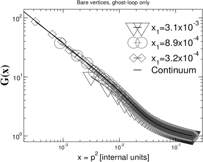
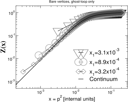
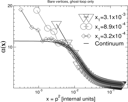
Figure 5.3: Shown are the ghost dressing function, $G(x)$, the gluon dressing function, $Z(x)$, and the running coupling, $\alpha(x)$, in the bare-vertex ghost-loop only truncation for different momentum grid spacings corresponding to different finite volumes of a torus. The fully drawn lines labelled continuum represent the respective results for continuous momenta.

5.3.2 Numerical solutions

Our results for the ghost dressing function, the gluon dressing function and the running coupling in the bare-vertex ’ghost-loop only’ and the dressed vertex truncation can be seen in Figs. 5.3 and 5.4. In both truncation schemes we solved for three different momentum spacings corresponding to different volumes in coordinate space. To keep the cutoff identical for all the spacings within each truncation scheme we have chosen three different grid sizes respectively. For the bare vertex truncation they are $N=17^{4},31^{4},51^{4}$ and for the dressed vertex truncation they are $N=21^{4},41^{4},61^{4}$.

     

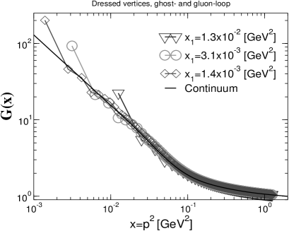
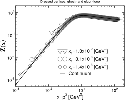
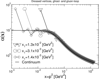
Figure 5.4: The same as Fig. 5.3 for the dressed vertex truncation.

The finite volume effects seen in both truncation schemes are very similar: Compared to the respective continuum solutions the ones obtained on a torus show deviations for the first few lattice points in the infrared. For large momenta all functions obtained on a torus approach the continuum ones. The biggest effect can be seen for the running coupling $\alpha$. As $\alpha(p^{2})$ is proportional to the product $Z(p^{2})G^{2}(p^{2})$ the deviations of the torus dressing functions from the continuum curves amplify in the infrared in a somewhat erratic way, such that the data points at small momenta cannot be connected by a smooth line. Comparing larger and smaller spacings of momentum grids one clearly sees that the effect is always one of the first spheres on the respective lattices and therefore moves to the infrared for smaller spacings.

The most important properties of the continuum solutions can still be found in the torus solutions despite some deviations in the infrared. Going from larger to smaller spacings a power-like behaviour of the dressing functions in the infrared with the correct exponents can still be inferred. For the truncation scheme with dressed vertices the gluon dressing function on the torus has the same shape and the same height of the bump in the bending region of the curve. This is a first central result of our investigation: Employing a torus as infrared regularisation is possible.

     

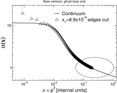
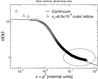
Figure 5.5: Here we compare the running coupling of the bare vertex ghost-loop only truncation for different treatments of the lattice cut-off, c.f. section 5.2. The torus curve on the left panel is calculated on a grid where the edges have been cut, whereas the coupling on the right panel is obtained on a full hypercubic grid. The ellipses mark the region where the latter treatment is inferior.

Before we move on to discuss the results in our novel truncation scheme we show what happens, if the four dimensional momentum grid is not cut at the edges according to the prescription discussed in section 5.2. In Fig. 5.5 we compare the running coupling of the bare vertex ’ghost-loop only’ truncation for different treatments of the lattice cut off. The torus curve in the left panel is calculated on a grid with edges cut, whereas the coupling on the right panel is obtained on a full hypercubic grid. Clearly one observes sizeable deviations in the ultraviolet behaviour of the latter curve compared to the continuum result. As explained in section 5.2 this is a result of breaking rotational symmetry on the lattice. On the inner, full hyperspheres we have the discrete rotational symmetry group Z(4) for very small discrete steps, whereas these steps become larger and larger for those hyperspheres which contain points on the edges of the lattice. Cutting these edges obviously improves the ultraviolet behaviour of our solutions.

The numerical results for our novel truncation scheme of chapter 3 with a transverse projector, $\zeta=1$, are shown in Fig. 5.6. At the time those results were found they have been the first numerical solutions at all in a truncation scheme without any angular approximations [83]. In the meantime, as we have seen in chapter 3, solutions for continuous momenta are also available [84]. Both calculations are compared in Fig. 5.6. For the presented torus solutions on three different volumes lattice sizes of $N=13^{4},43^{4},71^{4}$ have been used. As mentioned in the last subsection we did check cutoff effects by extrapolating the propagator functions at $z>\Lambda^{2}$ with a logarithmic tail with the correct anomalous dimensions. The results as compared to the ones obtained by simply setting $Z(z)=Z(\Lambda^{2})$ and $G(z)=G(\Lambda^{2})$ for all $z>\Lambda^{2}$ change by less than one per mille.

     

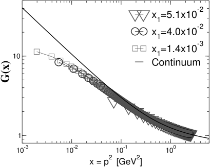
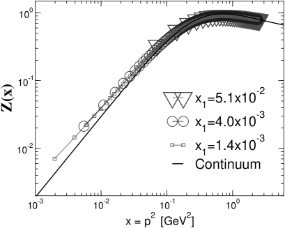
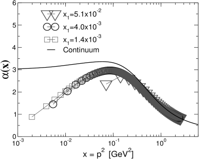
Figure 5.6: Here we present the ghost dressing function, $G(x)$, the gluon dressing function, $Z(x)$, and the running coupling, $\alpha(x)$, in the truncation scheme of chapter 3 for different volumes using a transverse projector, i.e. $\zeta=1$.

     

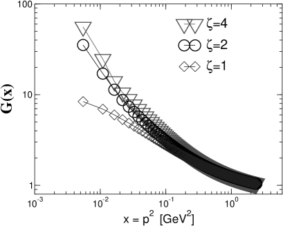
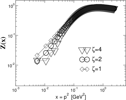
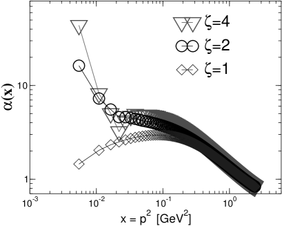
Figure 5.7: The same as Fig. 5.6 for different projectors. The corresponding solutions in the continuum are given in Fig. 3.5.

In section 3.3.2 we raised the question, which one out of two analytical solutions of the continuum DSEs in the infrared is connected to a full numerical solution for finite momenta. We have answered this question partially in section 3.4 where we showed that a numerical solution exists which connects to the infrared solution $\kappa=0.595$. However, in a numerical calculation in the continuum the analytical infrared solutions are used as input in the infrared and reproduced self-consistently. Thus one might argue that we showed the existence but not the uniqueness of the numerical solution with $\kappa=0.595$. On a torus we have no input in the infrared. Therefore a torus solution favours automatically the physical solution in the infrared, as we believe the infinite volume limit to be smooth. The results shown in Fig. 5.6 are clearly in agreement with the power behaviour $\kappa=0.595$ already found in the continuum and disfavours the second solution, $\kappa\approx 1.3$. The infrared critical exponent as calculated in refs. [62, 70], $\kappa=0.595$, thus has been verified.

The gluon dressing function in Fig. 5.6 is remarkably stable against changes of the volume and approaches more and more the expected power solution for small momenta, although this process seems to be very slow. For the ghost dressing function one observes deviations of the first points in the infrared: An extraction of the correct infrared critical exponent from the numerical solution for the ghost function is hardly possible. Only some points come close to the analytical value of the continuum before the curve starts bending down again for small momenta. For the extracted value of the running coupling in the infrared this leads to a distinct mismatch to what one is to expect on the basis of analytical results.

At first sight the fact that the power solution for the ghost dressing function could be not reproduced numerically to a reasonable precision may seem disappointing. Nevertheless these numerical results themselves show that the ghost dressing function is highly singular in the infrared. This reflects the long-range correlation of ghosts in Landau gauge. Therefore one should expect the ghost dressing function to be the one affected most by a finite volume. On the contrary the gluon dressing function vanishes in the infrared and consequently it is much less affected by a finite volume. We expect the ghost dressing function together with the running coupling to approach more and more the correct power solution in the infrared as lattice spacings are decreased and lattice sizes are increased.

       

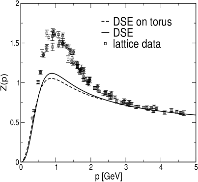
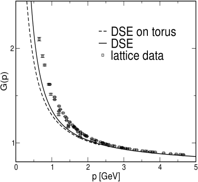
Figure 5.8: Results on the torus compared to recent lattice results [48, 49]. As the torus points are very close to each other on a linear momentum scale we did not resolve the torus curves into single points.

Furthermore, we add a remark on the transversality of the gluon propagator, c.f. the respective discussion in section 3.1. Our numerical results on a torus for different values of the parameter $\zeta$ can be seen in Fig. 5.7. Although the solutions show the expected dependence on the form of the projector this dependence is not too drastic and in general the behaviour of these different solutions is very similar. For the gluon dressing function one observes that the more $\zeta$ grows the greater is the deviation from the pure power behaviour and correspondingly from the continuum solutions, which have been shown in subsection 3.4.2. The points at small momenta cannot be connected by a smooth line any more. Based on the infrared analysis in subsection 3.3.2 one might anticipate that $\kappa$ should approach the value $\kappa=0.5$ more and more as $\zeta$ grows until there is a jump to the solution from $\kappa=0.5^{+}$ to $\kappa=1$ as the Brown–Pennington limit $\zeta=4$ is reached. We do not observe such a qualitative jump in our solutions on a torus. The solution shown for $\zeta=4$ is approached smoothly when $\zeta$ approaches this limit. This clearly indicates that the solution $\kappa=1$ might not exist at all if one removes the torus as a regulator.

Finally we compare our results of the new truncation scheme to recent SU(2) lattice calculations [49, 48], c.f. the corresponding comparison between lattice and DSE results in section 3.4.2. The two graphs in Fig. (5.8) suggest that the differences between our solutions in the continuum and on a torus are much smaller than the difference to the lattice result, at least for intermediate momenta. We explained in chapter 3 that this difference can be attributed to full two-loop contributions which are missed out in the DSE calculations but are certainly present in lattice Monte-Carlo simulations. For small momenta we see that our calculations on a torus employ much larger volumes than is possible in lattice simulations up to now. A thorough investigation of the infinite volume limit of the DSE solutions on a torus including a careful analysis of possible cut-off effects is certainly desirable and under way.

5.4 Summary

In this chapter we have presented numerical solutions of truncated systems of Dyson–Schwinger equations for the gluon and ghost propagators in Landau gauge SU(N) Yang–Mills theories. We have employed a four-torus, i.e. a compact space-time manifold, as an infrared regulator. Apart from the infrared finite volume effects encountered on such a manifold we found solutions on a torus which are very close to the ones obtained in the continuum formulation for various truncation schemes. Thus a central result of this chapter is: Dyson-Schwinger equations on a torus are feasible.

For small momenta we found the expected finite volume effects in the solutions of the DSEs on a torus. These deviations from the continuum results are somewhat erratic for the two truncation schemes employing an angular approximation in the sense that the values of the dressing functions on the momentum grid cannot be connected by a straight line. For our new truncation scheme without angular approximations this is different: systematic deviations from the continuum solutions occur. We find small deviations for the gluon dressing function and larger differences for the ghost dressing function on a torus compared to the continuum one. This is what one expects, since the infrared dominant ghost correlation is long ranged and should therefore be more affected by the finite volume than the gluon correlation.

Employing a torus as infrared regulator has certain advantages compared to the continuum formulation. In the numerical calculation of the continuum DSEs one has to match the analytically determined solution in the infrared carefully to the region where the dressing functions are determined numerically. On a torus the finite volume in coordinate space leads to a finite value of the smallest squared momentum encountered in the calculations. Thus one has not to worry about infrared singularities. Furthermore it is much easier to obtain convergence in the numerical iteration process. Historically we solved the truncation scheme introduced in chapter 3 on the torus first and only subsequently in the continuum using the torus solutions as start values in the iteration process. Thus the torus formulation is an important technical tool.

Furthermore we used the Dyson-Schwinger equations on a torus to corroborate a result of chapter 3: only one out of two analytical solutions from the infrared analysis of the continuum equation is connected to numerical results. For the transverse projection of the gluon equation this is the solution corresponding to $\kappa=0.595$. Such a statement is stronger if it is inferred from solutions on a torus than from corresponding continuum results. The reason is that we have to use the analytical infrared solution as self consistent input in the continuum calculations to obtain numerical stability. This is not the case on a torus.

Chapter 6 The coupled system of quark, gluon and ghost DSEs

In this chapter we will enlarge our focus from pure Yang-Mills theory to Landau gauge QCD. We will investigate the coupled system of Dyson-Schwinger equations for the ghost, gluon and the quark propagators. In the quark DSE we will study the mechanism by which physical quark masses are generated even though the bare quark masses in the Lagrangian are zero. This is a genuine effect of Strong QCD. It is well known that for vanishing bare masses the renormalised masses remain zero at each order of perturbation theory.

A thorough study of the infrared phenomena in the quark sector of QCD requires a continuum formulation. Lattice simulations of dynamical chiral symmetry breaking [117, 118, 119, 120, 121] have to deal with finite volume effects and in addition have to extrapolate from finite to zero quark mass. It is not possible to put massless quarks on a finite lattice. A recently performed study [119] in the overlap formalism e.g. employs masses in the range of $m_{0}=(126-734)\,\mbox{MeV}$. These values suggest that even the most elaborate extrapolation method to zero quark mass needs guidance and check from continuum results.

Apart from the phenomenon of mass generation we are interested in quark confinement. Single quark states have non-vanishing colour charge and are therefore not contained in the physical part of the state space of QCD. In subsection 2.3.2 we argued for a positive (semi-)definite metric in this physical subspace, whereas the remaining state space of QCD contains negative norm states as well. Consequently, negative norm contributions to the quark propagator are theoretical evidence for quark confinement.

The quark propagator is an important ingredient for many phenomenological models (see [9, 10, 122] and references therein). Thus, the quark DSEs have been studied extensively. Various ansätze for the gluon interaction in the quark equation have been explored. The resulting quark propagators have been used in bound state calculations based on the Bethe-Salpeter equations for mesons (see e.g. [28, 123, 124, 125, 126]) or Faddeev equations for baryons [127, 128, 129, 130, 131, 132, 133, 134, 135, 136, 137, 138]. One of the central aims of this thesis is to provide a solution for the quark propagator which incorporates the effects from the ghost and gluon DSEs directly and not via model assumptions.

This chapter is organised as follows: In the next section we will construct suitable ansätze for the quark-gluon vertex such that two important properties of the full quark DSE are reproduced: the independence of the generated quark mass from the renormalisation point and the asymptotic matching of the DSE-solutions to the results of perturbation theory. Fortunately, the corresponding DSEs for the fermions of QED are well studied (a short overview is given e.g. in [139]). We will dwell on these results and construct non-Abelian generalisations of Abelian vertices, which have the desired properties.

In the second section we present solutions for the quenched system of quark, ghost and gluon DSEs, i.e. we neglect the quark-loop in the gluon equation. A corresponding approximation is frequently used in lattice simulations. Comparing our solutions with recent lattice results [119] we find very good agreement for the quark propagator.

We then proceed to the unquenched case and incorporate the quark-loop into our truncation scheme for the ghost and gluon DSE from chapter 3. We present solutions for the full coupled system of DSEs for the quark, ghost and gluon propagators in the last section of this chapter. Compared to the quenched case we will find only moderate differences for the number of light flavours $N_{f}\leq 3$ [140].

6.1 The quark Dyson-Schwinger equation

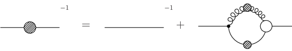
Figure 6.1: A diagrammatical representation of the quark Dyson-Schwinger equation.

We outlined the derivation of the Dyson-Schwinger equation for the quark propagator $S(p)$ at the end of section 2.4. The renormalised equation in flat Euclidean space-time is given by

$$S^{-1}(p)=Z_{2}\,S^{-1}_{0}(p)+\frac{g^{2}}{16\pi^{4}}\,Z_{1F}\,C_{F}\,\int d^{4}q\,\gamma_{\mu}\,S(q)\,\Gamma_{\nu}(q,k)\,D_{\mu\nu}(k)\,,$$ (6.1)

with the momentum routing $k=q-p$. The factor $C_{F}=(N_{c}^{2}-1)/2N_{c}$ in front of the integral stems from the colour trace of the loop. The symbol $\Gamma_{\nu}(q,k)$ denotes the full quark-gluon vertex. A diagrammatical representation of the equation is given in Fig. 6.1.

Suppressing colour indices the quark and gluon propagators in Landau gauge are given by

$$S(p) = \frac{1}{-ip\hskip-5.0pt/A(p^{2})+B(p^{2})}\>\>\>=\>\>\>A^{-1}(p^{2})\frac{ip\hskip-5.0pt/+M(p^{2})}{p^{2}+M^{2}(p^{2})}\,,$$ (6.2)

$$S_{0}(p) = \frac{1}{-ip\hskip-5.0pt/+m_{0}}\,,$$ (6.3)

$$D_{\mu\nu}(p) = \left(\delta_{\mu\nu}-\frac{p_{\mu}p_{\nu}}{p^{2}}\right)\frac{Z(p^{2})}{p^{2}}\,,$$ (6.4)

where the quark mass function $M$ is defined as $M(p^{2})=B(p^{2})/A(p^{2})$. For obvious reasons the dressing function $A(q^{2})$ is frequently called ’vector self energy’ and the dressing function $B(q^{2})$ ’scalar self energy’. Furthermore the inverse of the vector self energy, $1/A(q^{2})$, is denoted as ’quark wave function renormalisation’. The bare quark propagator $S_{0}(p^{2})$ contains the unrenormalised quark mass $m_{0}(\Lambda^{2})$ which depends on the cutoff $\Lambda$ of the theory. The bare mass is related to the renormalised mass $m_{R}(\mu^{2})$ via the renormalisation constant $Z_{m}$:

$$m_{0}(\Lambda^{2})=Z_{m}(\mu^{2},\Lambda^{2})\>m_{R}(\mu^{2})\,.$$ (6.5)

Here $\mu^{2}$ is the squared renormalisation point.

The renormalised and unrenormalised vector self energy, $A$ and $A_{0}$, are related by

$$A_{0}^{-1}(p^{2},\Lambda^{2})=Z_{2}(\mu^{2},\Lambda^{2})\>A^{-1}(p^{2},\mu^{2}).$$ (6.6)

In Landau gauge the quantum corrections to the vector self energy are finite. Correspondingly $Z_{2}(\mu^{2},\Lambda^{2})$ stays finite when the cutoff is sent to infinity and we have $0<Z_{2}(\mu^{2},\Lambda^{2})<1$. Furthermore the ghost-gluon vertex is not ultraviolet divergent in Landau gauge and we can choose $\tilde{Z}_{1}=1$, c.f. section 3.2. The Slavnov-Taylor identity for the quark-gluon vertex renormalisation factor $Z_{1F}$ thus simplifies,

$$Z_{1F}=\frac{\tilde{Z}_{1}Z_{2}}{\tilde{Z}_{3}}=\frac{Z_{2}}{\tilde{Z}_{3}}.$$ (6.7)

Previous studies of the quark equation in the so called Abelian approximation (an overview is given in ref. [9]) as well as the recent investigation in ref. [141] assume implicit cancellations between the full quark-gluon vertex, the dressed gluon propagator and the integral over the kernel of the DSE. Furthermore in the tensor structure of the quark-gluon vertex only a term proportional to $\gamma_{\mu}$ is employed.

In this thesis we do not have to rely on implicit cancellations since we calculated explicit solutions for the dressed gluon and ghost propagators, c.f. section 3.4.2. We will also construct explicit non-perturbative ansätze for the quark-gluon vertex including different tensor structures than $\gamma_{\mu}$. The advantages of such a treatment are obvious: every building block of the equation is explicitly given and well under control. We are able to assess the expedience of different vertex constructions. Furthermore the inclusion of several tensor structures in the vertex is supposed to be important in bound state calculations of scalar meson masses [143, 144]. Finally we hope providing an explicit construction of all parts of the quark equation leads in turn to more thorough statements on quark confinement.

In the following we assume an effective non-Abelian quark-gluon vertex of the form

$$\Gamma_{\nu}(q,k)=V_{\nu}^{abel}(p,q,k)\,W^{\neg abel}(p,q,k),$$ (6.8)

with $p$ and $q$ denoting the quark momenta and $k$ the gluon momentum. The non-Abelian factor $W^{\neg abel}$ multiplies an Abelian part $V_{\nu}^{abel}$, which carries the tensor structure of the vertex. This ansatz is motivated by the aim to respect gauge invariance as much as possible on the present level of truncation. The Slavnov-Taylor identity (STI) for the quark-gluon vertex is given by [7]

$$(-i)\>G^{-1}(k^{2})\>k_{\mu}\>\Gamma_{\mu}(q,p)=S^{-1}(p)\>H(q,p)-H(q,p)\>S^{-1}(q),$$ (6.9)

with the ghost dressing function $G(k^{2})$ and the ghost-quark scattering kernel $H(q,p)$. At present the non-perturbative behaviour of the ghost-quark scattering kernel is unknown. Therefore we cannot solve the STI explicitly. However, comparing the structure of eq. (6.9) with the corresponding Ward identity of QED,

$$(-i)\>k_{\mu}\>\Gamma_{\mu}^{QED}(q,p)=S^{-1}(p)-S^{-1}(q),$$ (6.10)

we are able to infer some information: Whereas the ghost fields of QED decouple from the theory and consequently do not show up in the Ward identity, there is an explicit factor of $G^{-1}(k^{2})$ on the left hand side of eq. (6.9). We therefore suspect the quark-gluon vertex of QCD to contain an additional factor of $G(k^{2})$ compared to the fermion-photon vertex of QED. Some additional ghost dependent structure seems necessary to account for the ghost-quark scattering kernel on the right hand side of eq. (6.9). For simplicity we assume the whole ghost dependence of the vertex to be contained in a non-Abelian factor multiplying an Abelian tensor structure.

The Abelian part of the vertex, $V_{\nu}^{abel}$, can be adopted from QED. The Ward identity (6.10) has long been solved [147, 148]. Furthermore transverse parts of the fermion-photon vertex have been fixed by Curtis and Pennington to satisfy multiplicative renormalisability in the Abelian fermion DSE for all linear covariant gauges [155, 156].

The non-Abelian factor $W^{\neg abel}$ is chosen such that the complete quark equation fulfils two conditions:

• The quark mass function $M(p^{2})$ should be independent of the renormalisation point $\mu^{2}$.

• The anomalous dimension $\gamma_{m}$ of the mass function known from resummed perturbation theory should be recovered in the ultraviolet.

In the course of this section we will prove the vertex ansatz

$$W^{\neg abel}(p,q,k) = G^{2}(z,s)\>\tilde{Z}_{3}(s,L)\>\frac{\left(G(z,s)\tilde{Z}_{3}(s,L)\right)^{-2d-d/\delta}}{\left(Z(z,s){Z}_{3}(s,L)\right)^{d}}\,,$$ (6.11)

$$V^{abel}_{\nu}(p,q,k) = \Gamma_{\nu}^{CP}(p,q,k)$$ (6.12)

$$= \frac{A(x,s)+A(y,s)}{2}\gamma_{\nu}$$

$$+\,\frac{A(x,s)-A(y,s)}{2(x-y)}(p\hskip-5.0pt/+q\hskip-5.0pt/)(p+q)_{\nu}+i\frac{B(x,s)-B(y,s)}{x-y}(p+q)_{\nu}$$

$$+\,\frac{A(x,s)-A(y,s)}{2}\left[(x-y)\gamma_{\nu}-(p\hskip-5.0pt/-q\hskip-5.0pt/)(p+q)_{\nu}\right]\times$$

$$\hskip 128.0374pt\frac{x+y}{(x-y)^{2}+(M^{2}(x)+M^{2}(y))^{2}}\,,$$

with the new parameter $d$ to satisfy the conditions (i) and (ii). To ease notation we used the abbreviations $x=p^{2}$, $y=q^{2}$ and $z=(p-q)^{2}$ for the squared momenta, also $s=\mu^{2}$ for the squared renormalisation point and $L=\Lambda^{2}$ for the squared cutoff of the theory. The anomalous dimension $\delta$ of the ghost propagator is $\delta=-9\>N_{c}/(44\>N_{c}-8\>N_{f})$ at one loop order for $N_{c}$ colours and $N_{f}$ flavours. The Abelian part of the vertex is given by the Curtis-Pennington (CP) vertex $\Gamma_{\nu}^{CP}(p,q,k)$.

From a systematic point of view the newly introduced parameter $d$ in the non-Abelian part of the vertex is completely arbitrary. Our numerical results, however, will indicate that values around the somewhat natural choice $d=0$ match best with lattice simulations, c.f. subsection 6.2.3.

If we would not care about (Abelian) gauge invariance we could also employ the much simpler vertex

$$W^{\neg abel}(p,q,k) = G^{2}(z,s)\>\tilde{Z}_{3}(s,\Lambda)\>\frac{\left(G(z,s)\>\tilde{Z}_{3}(s,L)\right)^{-2d-d/\delta}}{\left(Z(z,s)\>{Z}_{3}(s,L)\right)^{d}}$$

$$V^{abel}_{\nu}(p,q,k) = Z_{2}(s,L)\,\gamma_{\nu}$$ (6.13)

where we have taken the bare Abelian vertex, $\gamma_{\nu}$, multiplied with an extra factor of $Z_{2}$. In Landau gauge this construction also satisfies the conditions (i) and (ii), as will be shown in the next two subsections.

6.1.1 Multiplicative renormalisability of the quark equation

To proceed we substitute the vertex ansatz (6.13) into the quark equation (6.1). By taking the Dirac trace once with and once without multiplying the equation with $p\hskip-5.0pt/$ we project out the mass function $M(x)$ and the vector self energy $A(x)$. We arrive at

$$M(x)A(x,s) = Z_{2}(s,L)\>m_{0}(L)+\frac{Z_{2}(s,L)}{3\pi^{3}}\int d^{4}q\Bigg{\{}\frac{\alpha(z)}{z\>(y+M^{2}(y))}\>Z_{2}(s,L)\>A^{-1}(y,s)\times$$ (6.14)

$$\hskip 128.0374pt\frac{\left(G(z,s)\>\tilde{Z}_{3}(s,L)\right)^{-2d-d/\delta}}{\left(Z(z,s)\>{Z}_{3}(s,L)\right)^{d}}\>3M(y)\Bigg{\}}\,,$$

$$A(x,s) = Z_{2}(s,L)+\frac{Z_{2}(s,L)}{3\pi^{3}}\int d^{4}q\Bigg{\{}\frac{\alpha(z)}{x\>z\>(y+M^{2}(y))}\>Z_{2}(s,L)\>A^{-1}(y,s)\times$$

$$\hskip 28.45274pt\frac{\left(G(z,s)\>\tilde{Z}_{3}(s,L)\right)^{-2d-d/\delta}}{\left(Z(z,s)\>{Z}_{3}(s,L)\right)^{d}}\left(-z+\frac{x+y}{2}+\frac{(x-y)^{2}}{2\>z}\right)\Bigg{\}}\,,$$

where we have used the definition of the running coupling $\alpha$ in Landau gauge

$$\alpha(x)=\frac{g^{2}}{4\pi}\>Z(x,s)G^{2}(x,s)=\alpha(s)\>Z(x,s)\>G^{2}(x,s)\,,$$ (6.16)

c.f. eq. (3.21).

The behaviour of eqs. (6.14), (LABEL:bare-dse-a) under renormalisation can be explored by changing the renormalisation point $s=\mu^{2}$ to a new point $t=\nu^{2}$. We first note that the factor stemming from the non-Abelian part of the quark-gluon vertex is not affected by such a change:

$$\frac{\left(G(z,s)\>\tilde{Z}_{3}(s,L)\right)^{-2d-d/\delta}}{\left(Z(z,s)\>{Z}_{3}(s,L)\right)^{d}}=\frac{\left(G(z,t)\>\tilde{Z}_{3}(t,L)\right)^{-2d-d/\delta}}{\left(Z(z,t)\>{Z}_{3}(t,L)\right)^{d}}\,.$$

This can be seen easily with the help of the relations

$$G_{0}(x,L) = G(x,s)\>\tilde{Z}_{3}(s,L)\,,$$ (6.17)

$$Z_{0}(x,L) = Z(x,s)\>{Z}_{3}(s,L)\,,$$ (6.18)

between the unrenormalised and renormalised ghost and gluon dressing function, c.f. eq. (3.18). Furthermore the running coupling $\alpha(z)$ is independent of the renormalisation point, c.f. the discussion in subsection 3.2.2. From eq. (6.6) we infer

$$Z_{2}(t,L)\>A^{-1}(x,t)=Z_{2}(s,L)\>A^{-1}(x,s)\,.$$ (6.19)

With the renormalisation condition $A(t,t)=1$ we have

$$Z_{2}(t,L)=Z_{2}(s,L)\>A^{-1}(t,s)\,,$$ (6.20)

and subsequently

$$A(x,t)=A(x,s)\>A^{-1}(t,s)\,.$$ (6.21)

Substituting eqs. (6.20) and (6.21) into the Dyson-Schwinger equations (6.14) we find the mass function $M(x)$ to be independent of the renormalisation point, i.e. condition (i) is satisfied. Note that without the extra factor of $Z_{2}$ in the Abelian part of the vertex (6.13) we would violate this condition.

Figure 6.2: Sketch of a finite renormalisation from a perturbative point $s$ to a non-perturbative point $t$ for the vector self energy $A$.

Before we examine the case of the more sophisticated Curtis-Pennington type vertex (6.12), we mention two important points. First, according to perturbation theory we have $A(x\rightarrow\infty,s)\rightarrow 1$ and $Z_{2}(s,L)\rightarrow 1$ for large renormalisation points $s$. However, this is just a special case of the general relation

$$A(x\rightarrow\infty,s)\rightarrow Z_{2}(s,L)$$ (6.22)

which can be inferred from eqs. (6.20) and (6.21). In Fig. 6.2 we sketch the vector self energy renormalised at two different points $s$ and $t$, with $s$ in the perturbative and $t$ in the non-perturbative region of momentum. We will see a similar picture when we present our numerical solutions in section 6.2.3.

Second, the alert reader might worry about the appearance of the ghost and gluon renormalisation factors $Z_{3}(L)$ and $\tilde{Z}_{3}(L)$ in the interaction kernel of the quark equation. Certainly the renormalised functions $M(x)$ and $A(x)$ should not depend on the cutoff of the integral. The balance of cutoff dependent quantities in the equation is controlled by various factors of $Z_{2}(L)$ and $Z_{m}(L)$. We have to take care not to disturb this balance by the vertex ansatz. Thus the non-Abelian part of our quark-gluon vertex contains such powers of $Z_{3}(L)$ and $\tilde{Z}_{3}(L)$ that the cutoff dependence of these quantities cancel. This can be easily checked using the scaling behaviour

$$Z_{3}(s,L) = \left(\frac{\alpha(L)}{\alpha(s)}\right)^{\gamma}\,,$$

$$\tilde{Z}_{3}(s,L) = \left(\frac{\alpha(L)}{\alpha(s)}\right)^{\delta}\,,$$ (6.23)

of the renormalisation factors for $L\rightarrow\infty$ and the relation $\gamma+2\delta+1=0$, c.f. eq. (3.34).

Along the same lines as for the bare vertex construction we prove condition (i) for the Curtis-Pennington type vertex. Plugging eqs. (6.11), (6.12) into the quark equation (6.1) and projecting onto $M(x)$ and $A(x)$ we arrive at

$$M(x)A(x,s) = Z_{2}(s,L)m_{0}(L)+\frac{Z_{2}(s,L)}{3\pi^{3}}\int d^{4}q\frac{\alpha(z)}{z(y+M^{2}(y))}\frac{\left(G(z,s)\tilde{Z}_{3}(s,L)\right)^{-2d-d/\delta}}{\left(Z(z,s){Z}_{3}(s,L)\right)^{d}}$$ (6.24)

$$\times A^{-1}(y,s)\>\left[\frac{3}{2}(A(x,s)+A(y,s))M(y)\right.$$

$$\hskip 56.9055pt+\frac{1}{2}(\Delta A\>M(y)-\Delta B)\left(-z+2(x+y)-\frac{(x-y)^{2}}{z}\right)$$

$$\hskip 56.9055pt\left.+\frac{3}{2}(A(x,s)-A(y,s))M(y)\Omega(x,y)(x-y)\right]$$

$$A(x,s) = Z_{2}(s,L)+\frac{Z_{2}(s,L)}{3\pi^{3}}\int d^{4}q\frac{\alpha(z)}{xz(y+M^{2}(y))}\frac{\left(G(z,s)\tilde{Z}_{3}(s,L)\right)^{-2d-d/\delta}}{\left(Z(z,s){Z}_{3}(s,L)\right)^{d}}$$

$$\times A^{-1}(y,s)\>\left[\left(-z+\frac{x+y}{2}+\frac{(x-y)^{2}}{2z}\right)\frac{A(x,s)+A(y,s)}{2}\right.$$

$$\hskip 56.9055pt-\left(\frac{\Delta A}{2}(x+y)+\Delta B\>M(y)\right)\left(-\frac{z}{2}+(x+y)-\frac{(x-y)^{2}}{2z}\right)$$

$$\hskip 56.9055pt+\left.\frac{3}{2}(A(x,s)-A(y,s))M(y)\Omega(x,y)\left(\frac{x^{2}-y^{2}}{2}-z\frac{x-y}{2}\right)\right].$$

Here we have used the abbreviations

$$\Delta A = \frac{A(x,s)-A(y,s)}{x-y},$$

$$\Delta B = \frac{B(x,s)-B(y,s)}{x-y},$$

$$\Omega(x,y) = \frac{x+y}{(x-y)^{2}+(M^{2}(x)+M^{2}(y))^{2}}.$$

With the help of the relations (6.20) and (6.21) we find the quark equations (6.24), (LABEL:CP-A) to be consistently renormalised if and only if the scalar self energy behaves like

$$B(x,t)=B(x,s)\,A^{-1}(t,s)$$ (6.26)

and the mass function

$$M(x)=B(x,s)/A(x,s)$$ (6.27)

is independent of the renormalisation point.

Summing up the results of this subsection we have shown that both vertex constructions, eqs. (6.12) and (6.13), lead to a renormalisation point independent mass function as is required by condition (i) of section 6.1. The same is true for a Ball-Chiu type vertex, which is the Curtis-Pennington construction (6.12) without the transverse term proportional to $\Omega(x,y)$. Note that in different gauges than Landau gauge only the Curtis-Pennington construction would satisfy condition (i), similar to QED [155, 156].

6.1.2 Ultraviolet analysis of the quark equation

In this subsection we will show that the ansätze (6.12) and (6.13) for the quark-gluon vertex both lead to the correct perturbative limit of the quark mass function $M(x)$. We first examine the case of the bare vertex construction, eq. (6.14).

The ghost and gluon dressing functions $G$ and $Z$ are slowly varying for large momenta according to their perturbative limit given in eqs. (3.27), (3.28). For loop momenta $y$ larger than the external momentum $x$ we are therefore justified to employ the angular approximation $G(z),Z(z)\rightarrow G(y),Z(y)$, c.f. subsection 3.3.1. Furthermore there is a region $x_{0}<y<x$ where the approximation $G(z),Z(z)\rightarrow G(x),Z(x)$ is adequate. We are then able to carry out the angular integrals in eq. (6.14) with the help of the formulae given in appendix C.1. If we additionally take the external momentum $x$ to be large enough, then all masses in the denominators become negligible since the integral is dominated by loop momenta $y\approx x$. We then obtain

$$M(x)A(x,s) = Z_{2}(s,L)m_{0}(L)$$

$$+\,\frac{Z_{2}(s,L)}{\pi}\frac{\alpha(x)}{x}\>\int_{x_{0}}^{x}dy\>Z_{2}(s,L)\>A^{-1}(y,s)\>\frac{\left(G(z,s)\tilde{Z}_{3}(s,L)\right)^{-2d-d/\delta}}{\left(Z(z,s){Z}_{3}(s,L)\right)^{d}}M(y)$$

$$+\,\frac{Z_{2}(s,L)}{\pi}\int_{x}^{L}dy\frac{\alpha(y)}{y}\>Z_{2}(s,L)\>A^{-1}(y,s)\>\frac{\left(G(z,s)\tilde{Z}_{3}(s,L)\right)^{-2d-d/\delta}}{\left(Z(z,s){Z}_{3}(s,L)\right)^{d}}M(y)\,,$$

where the integral from $y=0$ to $y=x_{0}$ has already been neglected.

For large momenta $y>x_{0}$ the wave function renormalisation $A^{-1}$ and the renormalisation factor $Z_{2}$ cancel each other according to eq. (6.22). Furthermore we use the perturbative limit of the ghost and gluon dressing functions (c.f. eqs. (3.27), (3.28))

$$G(z) = G(s)\left[\omega\log\left(\frac{z}{s}\right)+1\right]^{\delta}\,,$$

$$Z(z) = Z(s)\left[\omega\log\left(\frac{z}{s}\right)+1\right]^{\gamma}\,,$$ (6.29)

with $\omega=\beta_{0}\alpha(s)/(4\pi)=(11N_{c}-2N_{f})\alpha(s)/(12\pi)$. If we additionally substitute the scaling behaviour of the renormalisation constants $Z_{3}$ and $\tilde{Z}_{3}$, eqs. (6.23), and exploit the relation $\gamma+2\delta+1=0$, eq. (3.34), we arrive at

$$M(x) = m_{0}(L)+\frac{1}{\pi}\frac{\alpha(x)}{x}\int_{x_{0}}^{x}dyM(y)+\frac{1}{\pi}\int_{x}^{L}dy\frac{\alpha(y)}{y}M(y)\,.$$ (6.30)

This well known equation describes the ultraviolet behaviour of the quark mass function. The classification of its solutions has been clarified by Miransky [157, 158], employing the perturbative form of the running coupling,

$$\alpha(y)=\alpha(s)\left[\omega\log\left(\frac{y}{s}\right)+1\right]^{-1}\,.$$ (6.31)

In the chiral limit, $m_{0}(L)=0$, we obtain the so called regular asymptotic form,

$$M(x)=\frac{2\pi^{2}\gamma_{m}}{3}\frac{-\langle\bar{\Psi}\Psi\rangle}{x\left(\frac{1}{2}\ln(x/\Lambda^{2}_{QCD})\right)^{1-\gamma_{m}}}\,.$$ (6.32)

Here $\langle\bar{\Psi}\Psi\rangle$ denotes the chiral condensate which is discussed in more detail in subsection 6.2.1. In the case of non-vanishing bare quark mass, $m_{0}(L)\neq 0$, the equation (6.30) is solved by the irregular asymptotic form,

$$M(x)=M(s)\left[\omega\log\left(\frac{x}{s}\right)+1\right]^{-\gamma_{m}}\,.$$ (6.33)

In this case we furthermore find

$$\gamma_{m} = \frac{12}{11N_{c}-2N_{f}}\,,$$ (6.34)

$$m_{0}(L) = M(s)\left[\omega\log\left(\frac{L}{s}\right)+1\right]^{-\gamma_{m}}\,,$$ (6.35)

in accordance with resummed perturbation theory.

We thus have shown that the bare vertex construction (6.13) admits a solution for the mass function $M(x)$, which has the correct perturbative behaviour for large momenta. A similar analysis is possible for the DSE with the Curtis-Pennington type vertex, eq. (6.24). As the vector self energy goes to a constant in the limit of large momenta, eq. (6.22), all terms proportional to $A(x)-A(y)$ are suppressed in this limit. Furthermore, according to the perturbative expression (6.33) the $\Delta B$-term contributes at most subleading logarithmic corrections in eq. (6.24). The first term in the brackets reduces to the bare vertex form because $A(x,s)\approx A(y,s)$ for large momenta $x,y$. Thus we obtain the same ultraviolet limit from eq. (6.24) than for the bare vertex construction. This is certainly also the case if a Ball-Chiu type vertex is employed.

6.2 The quark propagator in quenched QCD

In the course of this section we will compare our results for three different vertex types, which share the non-Abelian part proposed in eq. (6.11) but differ in their Abelian parts. We will employ the bare vertex, eqs. (6.13), and the Curtis-Pennington (CP) type vertex, eqs. (6.12). Furthermore we use a Ball-Chiu (BC) type construction, which employs only the first three terms of the CP-vertex. In Landau gauge all these vertex ansätze satisfy the conditions (i) and (ii) formulated in section 6.1. In order to compare the different vertex types on a quantitative level we will calculate the pion decay constant $f_{\pi}$ and the chiral condensate from the respective solutions for the quark mass function.

6.2.1 Pion decay constant, chiral condensate and quark masses

The pion decay constant is calculated from the Bethe-Salpeter equation (BSE), which describes the pion as bound state of quark and antiquark [125]. Apart from the dressed quark propagator the BSE involves couplings between quarks and gluons. On the level of the quark DSE we have substituted the full quark-gluon vertex by an vertex ansatz. However, at present it is only known for certain cases how such a vertex ansatz in the quark DSE translates to the corresponding quark-gluon coupling in the Bethe-Salpeter equation [159, 160]. No method is known up to know to derive the corresponding BSE for dressed quark-gluon vertices as the BC- or CP-vertex constructions.

We thus have to rely on the approximation

$$f_{\pi}^{2} = -\frac{N_{c}}{4\pi^{2}}\int dy\>y\>\frac{M(y)A^{-1}(y)}{(y+M^{2}(y))^{2}}\left(M(y)-\frac{y}{2}\frac{dM(y)}{dy}\right)\,,$$ (6.36)

which incorporates only the effects of the leading pion Bethe-Salpeter amplitude in the chiral limit [122]. From a comparison of the relative size of the amplitudes in model calculations [124, 143] one concludes that the approximation (6.36) should lead to an underestimation of $f_{\pi}$ by roughly ten percent.

The renormalisation point independent chiral condensate, $\langle\bar{\Psi}\Psi\rangle$, can be extracted from the ultraviolet behaviour of the quark mass function in the chiral limit (c.f. eq. (6.32)):

$$M(x)\,\stackrel{{\scriptstyle x\to L}}{{\longrightarrow}}\,\frac{2\pi^{2}\gamma_{m}}{3}\frac{-\langle\bar{\Psi}\Psi\rangle}{x\left(\frac{1}{2}\ln(x/\Lambda^{2}_{QCD})\right)^{1-\gamma_{m}}}\,.$$ (6.37)

Recall $x=p^{2}$ and $L=\Lambda^{2}$, where $\Lambda$ is the cutoff of our theory not to be confused with the scale $\Lambda_{QCD}$, which is to be taken from a fit to the running coupling, c.f. eqs. (3.57), (3.58).

The renormalisation point dependent chiral condensate $\langle\bar{\Psi}\Psi\rangle_{\mu}$ can be calculated via [125]

$$-\langle\bar{\Psi}\Psi\rangle_{\mu}:=Z_{2}(s,L)\,Z_{m}(s,L)\,N_{c}\,\mbox{tr}_{D}\int\frac{d^{4}q}{(2\pi)^{4}}S_{ch}(q^{2},s)\,,$$ (6.38)

where the trace is over Dirac indices, $S_{ch}$ is the quark propagator in the chiral limit and the squared renormalisation point is denoted by $s=\mu^{2}$. To one-loop order both expressions for the condensate are connected by

$$\langle\bar{\Psi}\Psi\rangle_{\mu}=\left(\frac{1}{2}\ln(\mu^{2}/\Lambda^{2}_{QCD})\right)^{\gamma_{m}}\langle\bar{\Psi}\Psi\rangle\,,$$ (6.39)

with the anomalous dimension $\gamma_{m}$ of the quark mass function.

For the calculation of the chiral condensate we first have to determine the mass renormalisation constant $Z_{m}(s,L)$. Recall the formal structure of the mass equation (6.14), which is given as

$$M(x)A(x,s)=Z_{2}(s,L)\,Z_{m}(s,L)\,m_{R}(s)+Z_{2}(s,L)\,\Pi_{M}(x,s)\,,$$ (6.40)

where $\Pi_{M}(x,s)$ represents the dressing loop. In order to extract $Z_{m}(s,L)$ from this equation we have to clarify the meaning of $m_{R}(s)$ which is related to the unrenormalised mass by

$$m_{0}(L)=Z_{m}(s,L)\,m_{R}(s),$$ (6.41)

c.f. eq. (6.5). Evaluating eq. (6.40) at the perturbative momentum $x=s$ the matter seems clear. We achieve consistency with eqs. (6.33) and (6.35), if

$$m_{R}(s) = M(s)\,,$$ (6.42)

$$Z_{m}(s,L) = \left[\omega\log\left(\frac{L}{s}\right)+1\right]^{-\gamma_{m}}\,,$$ (6.43)

which is indeed the correct perturbative scaling of the renormalisation constant $Z_{m}$ [9].

Certainly one could implicitly define the finite parts of $Z_{m}$ such that the relation (6.42) holds in general for all renormalisation points $s$. Then the parameter $m_{R}$ in the renormalised QCD-Lagrangian would already know about dynamical symmetry breaking. However, as the mass parameters of QCD are supposed to be generated in the electroweak sector of the standard model one could equally well argue that it is more systematic to exclude the effect of mass generation by strong interaction from $m_{R}$.

In our numerical calculations we will choose $s$ to be sufficiently large, therefore eq. (6.42) is valid anyway. Then $Z_{m}$ is determined by

$$Z_{m}(s,L) = \frac{M(x)\,A(x,s)-Z_{2}(s,L)\,\Pi_{M}(x,s)}{Z_{2}(s,L)\,M(s)}$$ (6.44)

$$= \frac{1}{Z_{2}(s,L)}-\frac{\Pi_{M}(s,s)}{M(s)}\,.$$

For the last equation we have set $x=s$ and have used the renormalisation condition $A(s,s)=1$.

In the numerical calculations we have to specify the masses $m_{R}(s)$ as input. Choosing a perturbative renormalisation point $s$ allows one to evolve the masses $m_{R}(s)$ to a different scale $t$ by

$$m_{R}(t)=m_{R}(s)\left(\frac{\ln(s/\Lambda_{QCD}^{2})}{\ln(t/\Lambda_{QCD}^{2})}\right)^{\gamma_{m}}.$$ (6.45)

For $t=(2\,\mbox{GeV})^{2}$ typical values for the masses of the light quarks are given by the Particle Data Group [102]:

$$\frac{1}{2}(m_{u}+m_{d})(2\,\mbox{GeV})\approx 4.5\mbox{MeV},\hskip 28.45274ptm_{s}(2\,\mbox{GeV})\approx 100\mbox{MeV}.$$ (6.46)

We will use similar masses in our calculations.

6.2.2 Renormalisation scheme and numerical method

In the quark equation we employ a MOM regularisation scheme similar to the one used in the ghost and gluon equations in chapter 3. The formal structure of the quark equation is given by

$$A(x,s) = Z_{2}(s,L)+Z_{2}(s,L)\,\Pi_{A}(x,s)\,,$$ (6.47)

$$M(x)A(x,s) = Z_{2}(s,L)\,Z_{m}(s,L)\,m_{R}(s)+Z_{2}(s,L)\,\Pi_{M}(x,s)\,.$$ (6.48)

We eliminate $Z_{2}$ from the first equation by isolating it on the left hand side and subtracting the same equation for $x=s$. With

$$\frac{1}{Z_{2}(s,L)}=\frac{1}{A(x,s)}+\frac{1}{A(x,s)}\Pi_{A}(x,s)\,,$$ (6.49)

we then have

$$\frac{1}{A(x,s)}=1-\frac{1}{A(x,s)}\Pi_{A}(x,s)+\Pi_{A}(s,s)\,,$$ (6.50)

using the renormalisation condition $A(s,s)=1$. In each iteration step we determine the vector self energy $A(x)$ from eq. (6.50) and subsequently $Z_{2}$ from eq. (6.49). For the mass function $M(x)$ we use

$$M(x)A(x,s)=Z_{2}(s,L)\,\Pi_{M}(x,s)$$ (6.51)

in the chiral limit and the subtracted equation

$$M(x)A(x,s)=M(s)+Z_{2}(s,L)\,\Pi_{M}(x,s)-Z_{2}(s,L)\,\Pi_{M}(s,s)$$ (6.52)

if chiral symmetry is broken explicitly, i.e. $m_{0}\not=0$.

For the numerical iteration we employ a Newton method and represent the dressing functions $A(x)$ and $M(x)$ with the help of Chebychev polynomials. Furthermore, we use a numerical infrared cutoff $\epsilon$, which is taken small enough for the numerical results to be independent of $\epsilon$. Numerical difficulties arise in the case of the Curtis-Pennington type vertex and even more for the Ball-Chiu construction. If the external momentum $x$ and the loop momentum $y$ are both small and close to each other then the derivative-like terms

$$\Delta A=\frac{A(x)-A(y)}{x-y},\hskip 56.9055pt\Delta B=\frac{B(x)-B(y)}{x-y},$$ (6.53)

are hard to evaluate accurately. Although the functions $A(x)$ and $B(x)$ are constant in the infrared and consequently should have derivatives close to zero one encounters large values for $\Delta A$ and $\Delta B$ due to numerical inaccuracies in $A$ and $B$. In order to evaluate $\Delta A$ and $\Delta B$ much more precisely at small momenta we fit the expressions

$$A(x)=\frac{A(0)}{1+a_{1}\,(x/\Lambda_{QCD}^{2})^{a_{2}}}\,,\hskip 28.45274ptB(x)=\frac{B(0)}{1+b_{1}\,(x/\Lambda_{QCD}^{2})^{b_{2}}}\,,$$ (6.54)

with the parameters $a_{1}$, $a_{2}$, $b_{1}$ and $b_{2}$ to the numerically evaluated functions. The scale $\Lambda_{QCD}=0.714\,\mbox{GeV}$ has been determined from our fits to the running coupling in section 3.4.2. For $x-y$ smaller than a suitable matching point we calculate the terms $\Delta A$ and $\Delta B$ from the fits. This procedure eliminates the numerical errors in the derivative terms and smoothes the numerical results considerably. In the case of the Ball-Chiu type vertex the iteration process does not converge unless we use these fits.

The renormalisation condition employed in the ghost-gluon system of equations is $G^{2}(s)Z(s)=1$ with $\alpha(s)=0.2$ at the squared renormalisation point $s=\mu^{2}$. Furthermore we choose the transversal tensor, $\zeta=1$, to contract the gluon equation, c.f. chapter 3. The physical scale in the quenched calculations is taken directly from the Yang-Mills results of section 3.4.2, i.e. we use the experimental value $\alpha(M_{Z}^{2})=0.118$ of the running coupling at the mass of the Z-boson to fix the scale.

6.2.3 Numerical results

	M(0)	$f_{\pi}$	$(-\langle\bar{\Psi}\Psi\rangle)^{1/3}$	$(-\langle\bar{\Psi}\Psi\rangle)^{1/3}$
	[MeV]	[MeV]	[MeV] (calc.)	[MeV] (fit)	$a_{1}$	$a_{2}$	$b_{1}$	$b_{2}$
bare vertex	177	38.5	162	160	3.05	0.99	0.06	1.00
CP d=$\delta$	150	50.5	223	225	-	-	-	-
BC-vertex	293	62.6	276	284	1.10	0.99	0.29	0.92
CP-vertex	369	78.7	303	300	0.83	0.99	0.20	1.00
CP d=0.1	464	87.5	334	330	0.79	0.99	0.34	0.95

Table 6.1: The mass $M(0)$, the pion decay constant $f_{\pi}$ calculated with eq. (6.36), the renormalisation point independent chiral condensate calculated with eqs. (6.38) and (6.39), and the condensate obtained by fitting the expression (6.37) to the chiral mass function in the ultraviolet for all four vertex types. Recall $\delta=-9/44$ in quenched approximation. If not stated otherwise the parameter $d$ in the vertex construction is taken to be $d=0$. For the case of the CP-vertex with $d=\delta$ we did not get good fits in the infrared.

In Fig. 6.3 we give our numerical solutions for the quark mass function and the inverse vector self energy in the chiral limit. We compare results obtained with five different ansätze for the quark-gluon vertex. For the generalised CP-vertex we investigate the ’natural’ case $d=0$, the value $d=\delta=-9/44$, already adopted in refs. [145, 146], and the value $d=0.1$. Furthermore we employed the bare vertex construction and a Ball-Chiu type vertex. The corresponding masses at the momentum $p^{2}=0$, the pion decay constant $f_{\pi}$, the renormalisation point independent chiral condensate and the fit parameters for the functions (6.54) are displayed in table 6.1.

The numerical results for the mass function all have a characteristic plateau in the infrared and show the regular asymptotic behaviour for large momenta, c.f. eq. (6.37). The bare vertex construction and the CP type vertex with $d=\delta$ both generate masses much smaller than typical phenomenological values of $300-400$ MeV. The BC- and the CP-type construction with $d=0$ provide good results, whereas the choice $d=0.1$ leads to a somewhat large mass. The lattice calculations taken from ref. [119] favour masses around $300$ MeV with the caveat that they are obtained by an extrapolation from sizeable bare quark masses to the chiral limit. The numerical solutions for the wave function renormalisation $1/A$ can be seen in the right diagram of Fig. 6.3. Whereas the ultraviolet asymptotic behaviour of all vertex constructions is similar we observe sizeable differences for small momenta. Again the bare vertex construction and the CP-vertex with $d=\delta$ are clearly disfavoured by the lattice data.

     

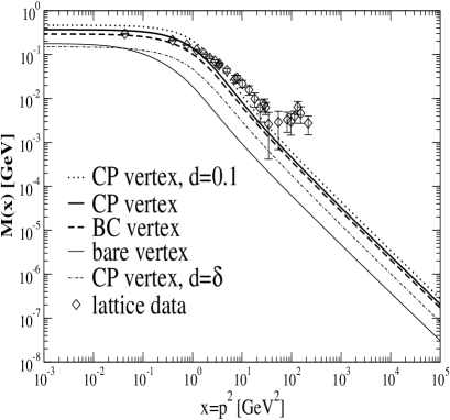
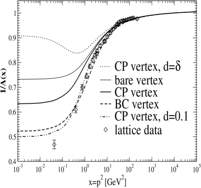
Figure 6.3: The mass function $M(x)$ and the inverse vector self energy $1/A(x)$ of a chiral quark are shown. We compare the results for five different vertices with lattice data taken from ref. [119].

     

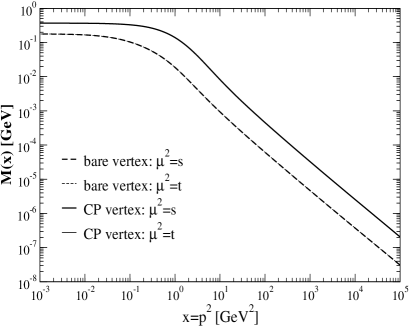
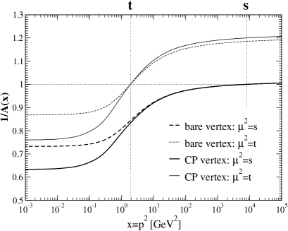
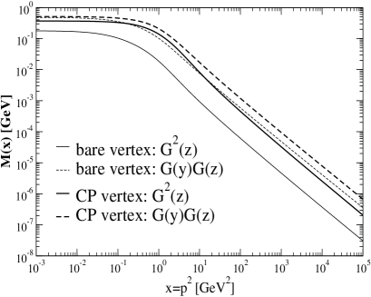
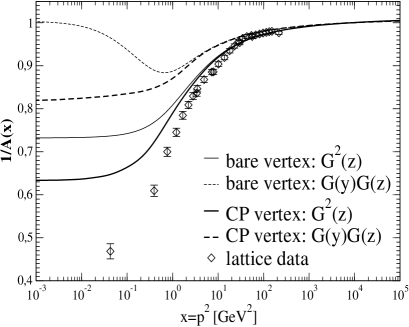
Figure 6.4: The behaviour of $M(x)$ and $1/A(x,s)$ under a change of the renormalisation point from $\mu^{2}=s$ to $\mu^{2}=t$.

     

Figure 6.5: In these diagrams we show that a change of arguments, $G^{2}(z)\rightarrow G(z)G(y)$, in the non-Abelian part of the quark-gluon vertex is disfavoured by lattice data.

Our approximate calculation of the pion decay constant should underestimate the experimental value $f_{\pi}=93\,\mbox{MeV}$ by about ten percent, c.f. the discussion below eq. (6.36). We thus have best results for the CP-vertex construction with $d=0$ and $d=0.1$. Furthermore we obtain very good agreement between the two different methods to extract the chiral condensate, c.f. subsection 6.2.1. Compared to the value $(-\langle\bar{\Psi}\Psi\rangle)^{1/3}=227\,\mbox{MeV}$ from the phenomenological study summarised in ref. [162] most of our results are larger.

Our favourite vertex for further investigations will be the CP-type construction. Although the bare vertex construction is by no means capable to reproduce phenomenological values of $M(0)$ and $f_{\pi}$ we will keep this vertex for the sake of comparison. However, we discard the BC-type vertex due to numerical problems in the infrared.

Apart from the case $d=\delta$ we obtain very good fits for the scalar and vector self energy, $A(x)$ and $B(x)$, for small momenta. The results for the fit parameters can be found in table 6.1. It is interesting to note that the exponents $a_{2}$ and $b_{2}$ in the fit functions of eq. (6.54) are all fitted very close to one. Such a behaviour might turn out to be crucial for the continuation of the quark propagator to negative $p^{2}$, i.e. timelike momenta, in future work.

A technical point is illustrated in Fig. 6.5. Here we display the dressing functions calculated with the bare vertex and the CP-vertex construction ($d=0$) for two different renormalisation points, $s=8100\,\mbox{GeV}^{2}$ and $t=1.9\,\mbox{GeV}^{2}$. Although these two points differ by three orders of magnitude the resulting mass functions for each vertex are indistinguishable in the plot. The wave function renormalisation $1/A(x,s)$ is multiplied by a constant factor when we change from $s$ to $t$, c.f. eq. (6.21). We thus find the behaviour expected from the discussion in subsection 6.1.1.

In Fig. 6.5 we compare the results for two different momentum assignments in the non-Abelian part of the vertex. We employ

$$W^{\neg abel}(x,y,z)=G^{2}(z,s)\>\tilde{Z}_{3}(s,L)\,,$$ (6.55)

in accordance with the $d=0$ case of eq. (6.11) and the modified assignment

$$W^{\neg abel}(x,y,z)=G(z,s)\>G(y,s)\>\tilde{Z}_{3}(s,L).$$ (6.56)

Both expressions behave similar under finite renormalisation and become equal in the limit of large momenta. Therefore both expressions lead to a mass function satisfying the conditions (i) and (ii) formulated in section 6.1. However, as can be seen from the plot, the lattice data for the wave function renormalisation $1/A$ clearly disfavour the second momentum assignment. This will be important in the next section, where we investigate the quark-loop in the gluon equation.

     

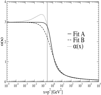
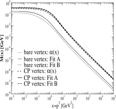
Figure 6.6: Results for three different forms of the running coupling in the quark equation: The running coupling calculated in chapter 3 and the two fits given in eqs. (3.57), (3.58).

Fig. 6.6 compares results for the bare vertex and the CP-type construction for three different forms of the running coupling in the interaction kernel of the quark equation. The two fit-functions, ’Fit A’ and ’Fit B’, have been given in eqs. (3.57), (3.58) Furthermore we used the running coupling calculated from the quenched ghost and gluon DSEs in section 3.4.2. Although there is the (presumably) artificial bump at $p^{2}\approx 0.1\,\mbox{GeV}^{2}$ in the running coupling, the mass functions obtained from the DSE-result and from ’Fit A’ are virtually indistinguishable. ’Fit B’, however leads to somewhat smaller masses. This observation suggests that nearly all the dynamically generated mass is produced from the integration strength above $p=500$ MeV, as is indicated by the vertical line in the plot of the running coupling. This is a favourable result as it would have been very unsatisfying if the artificial bump contributed a considerable amount to the quark mass function.

     

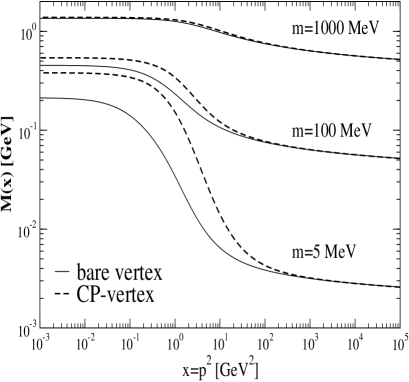
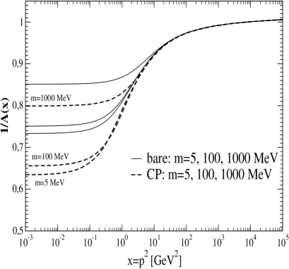
Figure 6.7: These diagrams show our results when three different bare quark masses are employed. In the diagram on the right small quark masses correspond to small values for $1/A$ in the infrared.

Finally we observe the effects of explicit chiral symmetry breaking in the plots of Fig. 6.7. We give results for three different quark masses, $m(2\,\mbox{GeV})=5$ MeV, $m(2\,\mbox{GeV})=100$ MeV and $m(1\,\mbox{GeV})=1000$ MeV. These values correspond roughly to the ones given by the Particle Data Group for the up/down-quark, the strange-quark and the charm-quark [102]. For small momenta we note again that the dressed vertex generates more mass in the quark equation than the bare vertex construction. This effect becomes much less dominant for the heavy quarks, where more and more of the infrared mass stems from explicit chiral symmetry breaking and not from dynamical mass generation. Furthermore in accordance with our analysis in subsection 6.1.2 we observe the same ultraviolet behaviour of the mass function for both vertex constructions.

6.3 Incorporating the quark-loop in the gluon equation

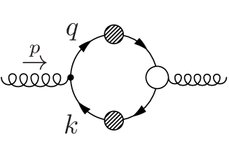
Figure 6.8: Diagrammatical representation of the quark-loop in the gluon equation.

In section 3.4.2 and in the last section we have discussed results for the ghost, gluon and quark propagators in quenched approximation. Now we go one step further and investigate the unquenched equations, i.e. we include the back-reaction of the quarks on the ghost-gluon system. To this end we incorporate the quark-loop in the truncation scheme developed in chapter 3. Due to our experience with the ghost- and gluon-loop this might seem to be a straightforward task. However, we will encounter some additional problems which are related to the quark-gluon vertex.

The contribution of the quark-loop to the gluon equation is given by

$$\Pi^{quark}_{\mu\nu}=-\frac{g^{2}N_{f}}{2(2\pi)^{4}}\,Z_{1F}\,\int d^{4}q\>\>\mbox{Tr}\left\{\gamma_{\mu}\,S(q)\,\Gamma_{\nu}(q,k)\,S(k)\right\},$$ (6.57)

where $x=p^{2}$ is the external gluon momentum and $y=q^{2}$ and $z=k^{2}=(q-p)^{2}$ are the squared momenta of the two quarks running in the loop. The trace is over Dirac indices.

In section 6.1 we have proposed an effective quark-gluon vertex $\Gamma_{\nu}(q,k)$ with Abelian and non-Abelian parts such that the quark equation is multiplicatively renormalisable and one-loop perturbation theory is recovered for large momenta. However, this construction is not capable to account as well for the one-loop behaviour of the unquenched gluon equation unless we switch the arguments of the non-Abelian part $W^{\neg abel}$, eq. (6.11), to different momenta. In the quark equation such a change of momentum leads to results clearly disfavoured by the lattice data, c.f. Fig. 6.5. We therefore have to use different momentum assignments for the quark-loop and the quark equation. Certainly, this is a deficiency which has to be resolved by a more elaborate vertex construction in future work. The aim of the present study, however, is to present an effective construction which captures essential properties of the theory.

Taking care of symmetries we propose the following ansatz for the non-Abelian part of the quark-gluon vertex in the quark-loop:

$$W^{\neg abel}_{quark-loop}(x,y,z) = G(y)G(z)\tilde{Z}_{3}(L)\frac{\left(G(y)\tilde{Z}_{3}(L)\right)^{-d-d/(2\delta)}}{\left(Z(y){Z}_{3}(L)\right)^{d/2}}\frac{\left(G(z)\tilde{Z}_{3}(L)\right)^{-d-d/(2\delta)}}{\left(Z(z){Z}_{3}(L)\right)^{d/2}}.$$

Here $x=p^{2}$ is the squared gluon momentum, $y=q^{2}$ and $z=k^{2}=(q-p)^{2}$ are the squared quark momenta, and $L=\Lambda^{2}$ is the squared cutoff. The Abelian part of the vertex is already symmetric with respect to the quark momenta.

Plugging the Curtis-Pennington type vertex into the quark-loop and contracting the free Lorenz-indices with the tensor (c.f. eq. (3.7))

$${\mathcal{P}}^{(\zeta)}_{\mu\nu}(p)=\delta_{\mu\nu}-\zeta\frac{p_{\mu}p_{\nu}}{p^{2}}\,,$$ (6.59)

we obtain

$$\Pi_{quark} = -\frac{g^{2}N_{f}}{(2\pi)^{4}}Z_{2}\int d^{4}q\frac{G(y)}{y+M^{2}(y)}\frac{G(z)}{z+M^{2}(z)}\frac{(G(y)\>G(z)\>\tilde{Z}_{3}^{2}(L))^{-d-d/(2\delta)}}{(Z(y)\>Z(z)\>Z_{3}^{2}(L))^{d/2}}\times$$

$$\times A^{-2}(y)A^{-2}(z)\>\left\{\frac{A(y)+A(z)}{2}\left(W_{1}(x,y,z)A(y)A(z)+W_{2}(x,y,z)B(y)B(z)\right)\right.$$

$$\hskip 85.35826pt+\frac{A(y)-A(z)}{2(y-z)}\left(W_{3}(x,y,z)A(y)A(z)+W_{4}(x,y,z)B(y)B(z)\right)$$

$$\hskip 85.35826pt+\frac{B(y)-B(z)}{y-z}\left(W_{5}(x,y,z)A(y)B(z)+W_{6}(x,y,z)B(y)A(z)\right)$$

$$\left.+\frac{(A(y)-A(z))(y+z)}{2((y-z)^{2}+(M^{2}(y)+M^{2}(z))^{2})}\left(W_{7}(x,y,z)A(y)A(z)+W_{8}(x,y,z)B(y)B(z)\right)\right\},$$

with the kernels

$$W_{1}(x,y,z) = \frac{\zeta z^{2}}{3x^{2}}+z\left(\frac{2-\zeta}{3x}-\frac{2\zeta y}{3x^{2}}\right)-\frac{2}{3}+\frac{(2-\zeta)y}{3x}+\frac{\zeta y^{2}}{3x^{2}}\,,$$ (6.61)

$$W_{2}(x,y,z) = \frac{2(4-\zeta)}{3x}\,,$$ (6.62)

$$W_{3}(x,y,z) = \frac{\zeta z^{3}}{3x^{2}}-z^{2}\left(\frac{1+\zeta}{3x}+\frac{\zeta y}{3x^{2}}\right)+z\left(\frac{1}{3}+\frac{(2\zeta-6)y}{3x}-\frac{\zeta y^{2}}{3x^{2}}\right)$$ (6.63)

$$+\frac{y}{3}-\frac{(\zeta+1)y^{2}}{3x}+\frac{\zeta y^{3}}{3x^{2}}\,,$$

$$W_{4}(x,y,z) = \frac{-2\zeta z^{2}}{3x^{2}}+z\left(\frac{4}{3x}+\frac{4\zeta y}{3x^{2}}\right)-\frac{2}{3}+\frac{4y}{3x}-\frac{2\zeta y^{2}}{3x^{2}}\,,$$ (6.64)

$$W_{5}(x,y,z) = \frac{\zeta z^{2}}{3x^{2}}-z\left(\frac{1+\zeta}{3x}+\frac{2\zeta y}{3x^{2}}\right)+\frac{1}{3}+\frac{(\zeta-3)y}{3x}+\frac{\zeta y^{2}}{3x^{2}}\,,$$ (6.65)

$$W_{6}(x,y,z) = \frac{\zeta z^{2}}{3x^{2}}-z\left(\frac{3-\zeta}{3x}+\frac{2\zeta y}{3x^{2}}\right)+\frac{1}{3}+\frac{(-\zeta-1)y}{3x}+\frac{\zeta y^{2}}{3x^{2}}\,,$$ (6.66)

$$W_{7}(x,y,z) = -\frac{z^{2}}{x}+z+\frac{y^{2}}{x}-y\,,$$ (6.67)

$$W_{8}(x,y,z) = 2\left(-\frac{z}{x}+\frac{y}{x}\right)\,.$$ (6.68)

Note that the symmetry factor $1/2$ and a factor $1/(3x)$ from the left hand side of the gluon equation have already been absorbed in the kernels. From this expression the corresponding one for the bare vertex construction can be read off easily by setting $W_{3-8}=0$ and replacing the remaining factor $(A(y)+A(z))/2$ in eq. (LABEL:quarkloop) by unity.

6.3.1 Ultraviolet analysis of the quark-loop

In section 3.3.1 we encountered quadratic divergences in the gluon equation for $\zeta\not=4$. These quadratic divergences occur in the ghost- and gluon-loop of the gluon equation and show up in the quark-loop as well. To identify such terms we expand the dressing functions in the integrand of the quark-loop around large loop momenta $y$ with the difference $(z-y)$ still larger than any quark mass. To leading order this expansion amounts in the replacements

$$G(z) \rightarrow G(y),$$

$$A(z) \rightarrow A(y),$$

$$\frac{A(y)-A(z)}{y-z} \rightarrow A^{\prime}(y),$$

$$\frac{B(y)-B(z)}{y-z} \rightarrow B^{\prime}(y),$$

$$\frac{(A(y)-A(z))(y+z)}{2((y-z)^{2}+(M^{2}(y)+M^{2}(z))^{2})} \rightarrow \frac{A^{\prime}(y)(y+z)}{2(y-z)},$$ (6.69)

with the derivatives $A^{\prime}$ and $B^{\prime}$. Note that the first two equations are identical to the angular approximation employed previously in subsection 3.3.1. For large momenta $x$ and $z$ the denominators in eq. (LABEL:quarkloop) simplify and the angular integrals are trivially performed using the integrals given in appendix C.1. We arrive at

$$\Pi_{quark}^{UV} = -\frac{g^{2}N_{f}}{16\pi^{2}}Z_{2}\int dy\>G^{2}(y)\>\frac{G(y)^{-2d-d/\delta}}{Z(y)^{d}}\>A^{-2}(y)\times$$ (6.70)

$$\hskip 54.06006pt\left\{A(y)\left(\frac{-2}{3y}+\frac{4-\zeta}{3x}+\frac{2(4-\zeta)}{3xy}M^{2}(y)\right)\right.$$

$$\hskip 54.06006pt+\frac{A^{\prime}(y)}{2}\left(\frac{1}{3}+\frac{-2(4-\zeta)y}{3x}+\left(\frac{-2}{3y}+\frac{2(4-\zeta)}{3x}\right)M^{2}(y)\right)$$

$$\hskip 54.06006pt+B^{\prime}(y)M(y)\left(\frac{2}{3y}-\frac{4-\zeta}{3x}\right)\left.+\frac{A^{\prime}(y)}{2}\left(\frac{4y}{x}-1+\frac{4}{x}M^{2}(y)\right)\right\}.\hskip 31.2982pt$$

Keeping in mind a factor $(1/y)$ hiding in the derivatives we are now able to identify three quadratically divergent terms: $(4-\zeta)/3x$ in the second line, $-2(4-\zeta)y/3x$ in the third line and $4y/x$ in the last line. The first two of them are proportional to $(4-\zeta)$ and reminds us of similar terms occurring in eq. (3.31). These terms are artefacts of the regularisation and will be subtracted from the kernels. However, we encounter the additional $\zeta$-independent quadratic divergent term $4y/x$ originating from the transverse part of the Curtis-Pennington vertex. Such a term is already known from corresponding studies in QED [169]. Although first suggestions have been made how the Curtis-Pennington vertex should be modified to avoid this problem [139], a convincing solution has not been found yet. In this thesis we therefore choose the pragmatic strategy of subtracting this term by hand together with the other quadratically divergent parts.

Moreover we subtract all further terms proportional to $(4-\zeta)$. Although these terms are not quadratically divergent they are artefacts of the regularisation. We then obtain a $\zeta$-independent expression for the quark loop at large momenta. Together with the corresponding expressions for the ghost-loop and the gluon-loop, eq. (3.31), we obtain a transversal gluon propagator in the ultraviolet as it should be the case in Landau gauge.

Collecting all modifications together we arrive at the new kernels

$$\widetilde{W}_{1}(x,y,z) = W_{1}(x,y,z)-\frac{(y+z)(4-\zeta)}{6x},$$ (6.71)

$$\widetilde{W}_{2}(x,y,z) = 0,$$ (6.72)

$$\widetilde{W}_{3}(x,y,z) = W_{3}(x,y,z)+\frac{2zy(4-\zeta)}{3x},$$ (6.73)

$$\widetilde{W}_{4}(x,y,z) = W_{4}(x,y,z)-\frac{(y+z)(4-\zeta)}{3x},$$ (6.74)

$$\widetilde{W}_{5}(x,y,z) = W_{5}(x,y,z)-\frac{(y+z)(4-\zeta)}{6x},$$ (6.75)

$$\widetilde{W}_{6}(x,y,z) = W_{6}(x,y,z)-\frac{(y+z)(4-\zeta)}{6x},$$ (6.76)

$$\widetilde{W}_{7}(x,y,z) = W_{7}(x,y,z)-\frac{(y-z)(y+z)}{x},$$ (6.77)

$$\widetilde{W}_{8}(x,y,z) = W_{8}(x,y,z).$$ (6.78)

Note that the subtracted terms are chosen to preserve the symmetry of the kernels with respect to the squared quark momenta $y$ and $z$.

Without quadratic divergences we are in a position to extract the leading logarithmic divergence of the quark-loop. With modified kernels the ultraviolet limit of the quark-loop is given by

$$\Pi_{quark}^{UV} = -\frac{g^{2}N_{f}}{16\pi^{2}}Z_{2}\int dy\>G^{2}(y)\>\frac{G(y)^{-2d-d/\delta}}{Z(y)^{d}}\>A^{-2}(y)\times$$ (6.79)

$$\hskip 71.13188pt\left\{A(y)\frac{-2}{3y}+\frac{A^{\prime}(y)}{2}\left(\frac{1}{3}+\frac{-2}{3y}M^{2}(y)\right)\right.$$

$$\hskip 71.13188pt+B^{\prime}(y)M(y)\frac{2}{3y}\left.+\frac{A^{\prime}(y)}{2}\left(-1+\frac{4}{x}M^{2}(y)\right)\right\}.$$

Similar to the situation in the DSE for the quark mass function, c.f. subsection 6.1.2, the leading ultraviolet term is the first term in the curly brackets. Substituting the ultraviolet limit of the vector self energy, eq. (6.22), the ghost and gluon dressing functions, eqs. (6.29), and choosing the perturbative renormalisation condition $G(s)=Z(s)=1$ we arrive at

$$\Pi_{quark}^{UV}=\frac{2N_{f}}{3(2\delta+1)\omega}\frac{g^{2}}{16\pi^{2}}\left\{\left[\omega\log\left(\frac{L}{s}\right)+1\right]^{2\delta+1}-\left[\omega\log\left(\frac{x}{s}\right)+1\right]^{2\delta+1}\right\}.$$ (6.80)

Here we have $\omega=\beta_{0}\alpha(s)/(4\pi)=(11N_{c}-2N_{f})\alpha(s)/(12\pi)$. Moreover $\delta$ is the anomalous dimension of the ghost propagator which is related to the corresponding anomalous dimension of the gluon by $\gamma+2\delta+1=0$, c.f. eq. (3.34). Combining the expression (6.80) with the results for the ghost and gluon loop, eq. (3.33) we obtain the anomalous dimensions

$$\gamma = \frac{-13N_{c}+4N_{f}}{22N_{c}-4N_{f}}$$ (6.81)

$$\delta = \frac{-9N_{c}}{44N_{c}-8N_{f}}$$ (6.82)

which are in accordance to one-loop perturbation theory for arbitrary numbers of colours $N_{c}$ and flavours $N_{f}$.

6.3.2 Infrared analysis of the quark-loop

In section 3.3.2 we employed the power law ansatz

$$Z(x)=Ax^{2\kappa},\hskip 28.45274ptG(x)=Bx^{-\kappa},$$ (6.83)

for the ghost and gluon dressing functions at small momenta $x$. Substituting this ansatz into the gluon equation we have found the ghost loop to be proportional to $x^{-2\kappa}$, dominating the gluon-loop in the infrared. When we compare our expression for the quark-loop, eq. (LABEL:quarkloop), with the ghost loop in eq. (3.25) we find two ghost dressing functions, $G(y)$ and $G(z)$, in each loop respectively. However, as the momenta $y$ and $z$ in the denominators of the quark loop are negligible compared to the quark masses in the infrared we anticipate that the quark-loop is less divergent than the ghost-loop for small momenta, provided the parameter $d$ is small.

An explicit calculation along the lines of our analysis in subsection 3.3.2 and appendix C.3 shows that the quark loop is proportional to $x^{-2\kappa+2+\kappa d/\delta}$ in the infrared. Therefore the quark loop is suppressed for small momenta provided the parameter $d$ fulfils the condition

$$d<\frac{-2\delta}{\kappa}.$$ (6.84)

As we have $\kappa\approx 0.5953$ and $\delta=-1/4$ for $N_{c}=3$ and $N_{f}=3$ we find the condition $d<0.84$, which is satisfied for all quark-gluon vertices employed in our calculation. From a numerical point of view we encounter serious instabilities in the quark and the gluon equation once $d$ is taken to be larger than $d\approx 0.2$.

We conclude that the quark-loop does not change the infrared behaviour of the ghost and gluon dressing functions found in section 3.3.2. In pure Yang-Mills theory as well as in QCD we thus have an infrared finite or vanishing gluon propagator and a ghost propagator which is more divergent than a simple pole. The Kugo-Ojima confinement criterion and Zwanziger’s horizon condition are both fulfilled not only in pure Yang-Mills theory but also in QCD. This is a central result of this chapter.

6.4 Numerical results

The numerical treatment of the integrals in the quark, ghost and gluon equations has been described in subsections 3.4.1 and 6.2.2. The iteration process is done for the ghost-gluon system and the quark equations separately: we first iterate the $N_{f}$ mutually uncoupled quark systems until convergence is achieved, feed the output into the ghost and gluon system, iterate until the ghost-gluon system converges, feed the output back into the quark equations and so on, until complete convergence of all equations is achieved. Similar to the quenched calculations we used $\alpha(s)=0.2$ at the renormalisation point $s=\mu^{2}$, and a transverse tensor to contract the gluon equation, $\zeta=1$.

In contrast to section 6.2 we fix the physical scale of the system not by the condition $\alpha(M_{Z}^{2})=0.118$ but by adjusting the pion decay constant to the experimental value. This choice has an important advantage: Whereas the asymptotic behaviour of the running coupling depends strongly on $N_{f}$ via the coefficient $\beta_{0}$ (c.f. appendix A.2), the pion decay constant turns out to be almost independent of $N_{f}$. In order to be able to compare different constructions for the quark-gluon vertex we fix the scale by requiring $f_{\pi}=85$ MeV for the CP-construction with $d=0.1$ and keep this scale when employing other vertices.

	M(0)		$f_{\pi}$		$(-\langle\bar{\Psi}\Psi\rangle)^{1/3}$		$\alpha(M_{Z})$		$\Lambda_{QCD}^{MOM}$
	[MeV]		[MeV]		[MeV]		-		[MeV]
vertex	qu.	unqu.	qu.	unqu.	qu.	unqu.	qu.	unqu.	qu.	unqu.
bare d=0	172	169	37.4	37.2	155	162	0.116	0.144	694	718
CP d=$\delta$	146	153	49.1	49.8	219	215	0.116	0.138	694	578
CP d=0	358	346	76.5	76.2	291	295	0.116	0.141	694	644
CP d=0.1	451	425	85.0	85.0	321	325	0.116	0.143	694	669

Table 6.2: A comparison between the quenched (qu.) and unquenched (unqu.) results for the quark mass M(0), the pion decay constant $f_{\pi}$, the renormalisation point independent chiral condensate, the running coupling at the mass of the Z-boson and $\Lambda_{QCD}^{MOM}$ for different vertices and values of the parameter $d$. The unquenched calculations are done for $N_{f}=3$ chiral quarks. Furthermore we have $\delta=-9N_{c}/(44N_{c}-8N_{f})=-0.25$ in the present case.

     

     

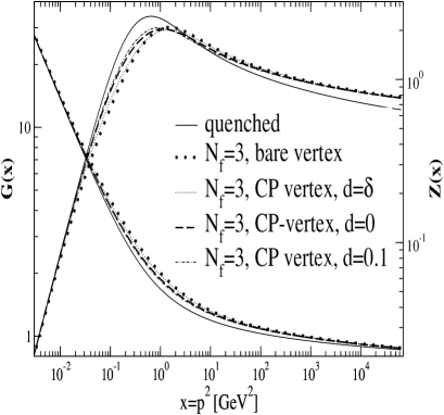
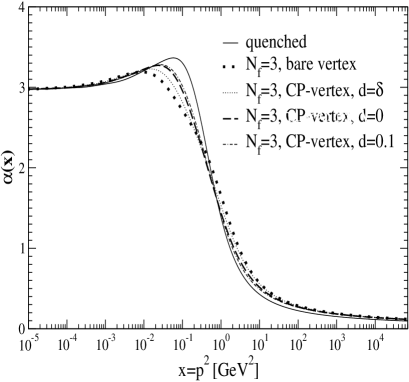
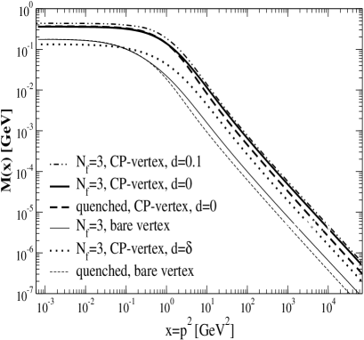
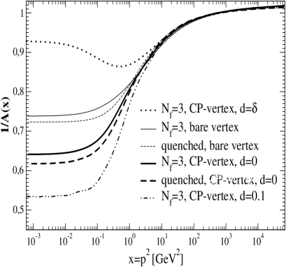
Figure 6.9: Displayed are the ghost and gluon dressing function, $Z$ and $G$, the running coupling $\alpha$, the quark mass function $M$ and the inverse vector self energy $1/A$. The calculations are done quenched and unquenched with $N_{f}=3$ quarks in the chiral limit.

     

         

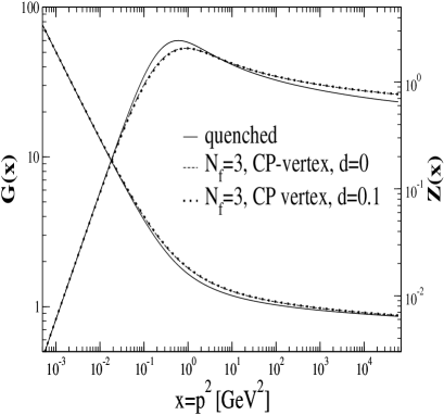
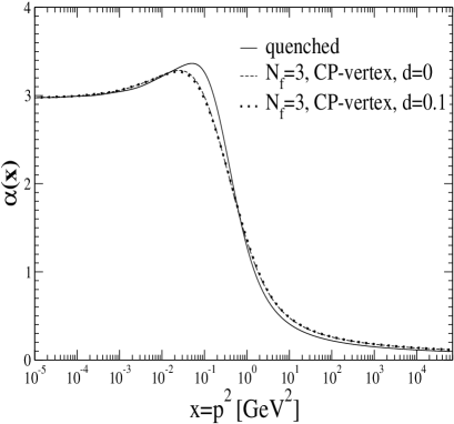
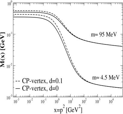
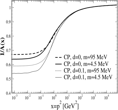
Figure 6.10: Results from the unquenched calculation with $N_{f}=3$ massive quarks. We used the renormalised masses $m_{u/d}(2\,\mbox{GeV})\approx 4.5$ MeV and $m_{s}(2\,\mbox{GeV})\approx 95$ MeV.

In table 6.2 we compare results for the quenched and unquenched system of equations, c.f. section 6.2. The quark mass, the pion decay constant and the chiral condensate differ only slightly for each vertex construction respectively. The only sizeable difference occurs in the running coupling. As expected from perturbation theory the unquenched running for $N_{f}=3$ results in larger values of the running coupling at $p^{2}=(M_{Z})^{2}$ compared to the quenched case $N_{f}=0$. We obtain $\alpha(M_{z})\approx 0.140$, which is somewhat larger than usually quoted values from experiment. If we increase the number of flavours in our calculation we encounter large numerical uncertainties and do not obtain convergence for $N_{f}\geq 5$.

All employed vertex constructions allow for nontrivial solutions of the quark equation corresponding to dynamical chiral symmetry breaking. However, similar to the quenched case the bare vertex construction and the CP-type vertex with $d=\delta$ generate much too small quark masses compared with typical phenomenological values. For $d=0$ we obtain good results for the quark mass, the pion decay constant and the chiral condensate, whereas the choice $d=0.1$ leads to somewhat large values. It is interesting to note that $d=0$ of all values is preferred as in this case the quark equation resembles most the fermion equation of QED.

In Fig. 6.9 we display the ghost, gluon and quark dressing functions corresponding to the unquenched and two representative quenched cases in table 6.2. We find different anomalous dimensions in the ultraviolet corresponding due to the change from $N_{f}=0$ to $N_{f}=3$, c.f. eqs. (6.29), (6.32), (6.82). As expected from the infrared analysis in subsection 6.3.2 the back-reaction of the quark-loop in the gluon equation does not affect the infrared behaviour of the ghost and gluon dressing functions. Consequently the infrared fixed point of the running coupling is the same as in pure Yang-Mills theory. Thus the Kugo-Ojima confinement criterion and Zwanziger’s horizon condition, c.f. section 2.3, are satisfied in quenched and unquenched Landau gauge QCD.

Our results for the case of explicitly broken chiral symmetry are shown in Fig. 6.10. We choose $N_{f}=3$ with renormalised quark masses corresponding to $m_{u/d}(2\,\mbox{GeV})=(4.4-4.6)$ MeV and $m_{s}(2\,\mbox{GeV})=(90-95)$ MeV. These masses are well in the range suggested by the Particle Data Group [102]. Compared to the chiral case the behaviour of the ghost and gluon dressing functions hardly changes. For the quark mass function we obtain the irregular asymptotic solution in the ultraviolet as expected from the analysis in subsection 6.1.2.

Furthermore we provide fits to our results for the quark propagator employing the fit functions

$$M(x) = \frac{1}{g_{1}+(x/\Lambda^{2}_{QCD})^{g_{2}}}\Bigg{(}g_{1}\,M(0)+$$ (6.85)

$$\left.\hskip 56.9055pt\hat{m}\left[\frac{2}{\ln(x/\Lambda^{2}_{QCD})}-\frac{2}{(x/\Lambda^{2}_{QCD})-1}\right]^{\gamma_{m}}(x/\Lambda^{2}_{QCD})^{g_{2}}\right)\,,\hskip 28.45274pt$$

$$\left[A(x)\right]^{-1} = \frac{\left[A(0)\right]^{-1}+h_{1}\,(x/\Lambda^{2}_{QCD})+h_{2}\,(x/\Lambda^{2}_{QCD})^{2}}{1+h_{3}\,(x/\Lambda^{2}_{QCD})+h_{4}\,(x/\Lambda^{2}_{QCD})^{2}}\,,$$ (6.86)

with $x=p^{2}$ and the six parameters $g_{1},g_{2},h_{1},h_{2},h_{3},h_{4}$. We used the renormalisation point independent current-quark mass $\hat{m}$, which is related to the renormalised mass $M(s)$ by

$$\hat{m}=M(s)\,\left(\frac{1}{2}\ln[s/\Lambda^{2}_{QCD}]\right)^{\gamma_{m}}\,,$$ (6.87)

to one loop order. For the running coupling, the ghost and the gluon dressing function we use the form ’Fit B’, given in eq. (3.58) and the fit functions from eqs. (3.59). In table 6.3 we give our values for all parameters as well as the numerical results for $M(0)$ and $[A(0)]^{-1}$. Note that the scale $\Lambda_{QCD}^{MOM}$ is different to the corresponding scale in the chiral limit due to the different ultraviolet behaviour of the quark-loop when quarks with non-vanishing bare masses are employed. When plotted the fits are virtually indistinguishable from our results in Fig. 6.10.

	$\Lambda^{MOM}_{QCD}$	a	b	c	d	$m_{R}$	$\hat{m}$	M(0)	$g_{1}$	$g_{2}$
	[MeV]					[MeV]	[MeV]	[MeV]
CP d=0	600	1.35	1.04	1.36	1.81	4.4	4.6	354	2.30	1.29
						90	96	507	3.42	1.09
CP d=0.1	620	1.32	1.06	1.42	1.78	4.5	4.6	429	2.22	1.28
						95	96	564	3.80	1.14

	$m_{R}$	$\left[A(0)\right]^{-1}$	$h_{1}$	$h_{2}$	$h_{3}$	$h_{4}$
	[MeV]
CP d=0	4.4	0.638	0.503	5.263$\times 10^{-3}$	0.544	5.202$\times 10^{-3}$
	90	0.671	0.305	1.420$\times 10^{-3}$	0.321	1.402$\times 10^{-3}$
CP d=0.1	4.5	0.538	0.448	2.740$\times 10^{-3}$	0.477	2.706$\times 10^{-3}$
	95	0.590	0.303	1.051$\times 10^{-3}$	0.317	1.037$\times 10^{-3}$

Table 6.3: Parameters for the fits to the unquenched results with $N_{f}=3$, $\alpha(s)=0.2$, $\delta=-0.25$, $\gamma_{m}=12/27$ and $\beta_{0}=27/3$.

     

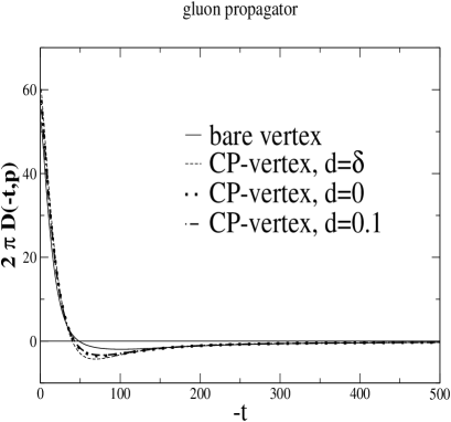
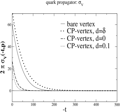
Figure 6.11: Here we display the one dimensional Fourier transforms of the gluon propagator, $D(-t,\vec{p}^{2})$, and the vector part of the quark propagator, $\sigma_{V}(-t,\vec{p}^{2})$. We observe violation of reflection positivity for the gluon propagator but not for the quark propagator.

Unquenched lattice calculations employing dynamical quarks are complex and time consuming [170]. To our knowledge such simulations for the propagators of QCD have not yet been performed. From our results in the Dyson-Schwinger approach we do not expect drastic differences between quenched and unquenched propagators on the lattice.

Finally, we investigate positivity violations in the gluon and quark propagators. Recall from our discussion in subsection 2.3.2 that the condition

$$\int_{0}^{\infty}dt\;dt^{\prime}\;\bar{f}(t^{\prime},\vec{p})\;S(-(t+t^{\prime}),\vec{p})\;f(t,\vec{p})\;<0$$ (6.88)

is sufficient for a given propagator $S$ to violate the reflection positivity axiom of Euclidean quantum field theory. Here $f$ are complex valued test functions, c.f. subsection 2.3.2. The one-dimensional Fourier transform $S(t,\vec{p})$ of the propagator $S(p_{0},\vec{p})$ is given by

$$S(t,\vec{p}):=\int\frac{dp_{0}}{2\pi}\,S(p_{0},\vec{p})\,e^{ip_{0}t}.$$ (6.89)

Provided there is a region around $t_{0}$ where $S(-t_{0},\vec{p})<0$ one can choose a real test function $f(t)$ which peaks strongly at $t_{0}$ to show positivity violation. In Fig. 6.11 we display the Fourier transform of the nontrivial part $D(p^{2})=Z(p^{2})/p^{2}$ of the gluon propagator and the vector part $\sigma_{V}(p^{2})=A(p^{2})/(p^{2}A(p^{2})+B(p^{2})$ of the quark propagator (we chose $\vec{p}^{2}=0$). Clearly the Fourier transform of the gluon propagator is negative on a large interval. The resulting positivity violation for the transverse gluon propagator in Landau gauge can be interpreted as a signal for gluon confinement, c.f. subsection 2.3.2. Note that the ghost propagator violates positivity trivially for $G(p^{2})>0$ as can be seen from the definition in eq. (3.3). From the Fourier transforms of $\sigma_{V}(p^{2})$ displayed in the second diagram of Fig. 6.11 we cannot conclude positivity violation for the quark propagator. As we have an indefinite metric in the unphysical part of the state space of QCD this result is not in contradiction with quark confinement. In addition we have to keep in mind that eq. (6.88) is a sufficient but not a necessary condition for the violation of positivity. Further investigations of the quark propagator will be done in future work.

6.5 Summary

In this chapter we have presented solutions of the (truncated) Dyson-Schwinger equations for the propagators of Landau gauge QCD. We first concentrated on the Dyson-Schwinger equation for the quark propagator. We proposed several ansätze for the quark-gluon vertex which consist of an Abelian part carrying the tensor structure of the vertex and a non-Abelian multiplicative correction. Our guiding principles for the construction of these vertices have been two important conditions on the truncated quark equation: it should be multiplicatively renormalisable and recover perturbation theory for large external momenta. We showed that the resulting quark mass function is independent of the renormalisation point and has the correct asymptotic behaviour for large momenta.

In the quark equation both the ghost and gluon dressing function show up at least implicitly. In the quenched approximation we employ our solutions of the ghost and gluon Dyson-Schwinger equations in the truncation scheme of chapter 3. In the unquenched calculations we include the back-reaction of the quarks on the ghost and gluon system and solve the quark, gluon and ghost Dyson-Schwinger equations self-consistently.

All our solutions show dynamical chiral symmetry breaking. However, only carefully constructed vertex ansätze have been able to generate masses in the typical phenomenological range of $300-400$ MeV. Constructions with an Abelian part satisfying the Abelian Ward-identity are superior to other vertex ansätze. We obtained very good results for the quark mass, the pion decay constant and the chiral condensate by employing a generalised Curtis-Pennington vertex. In the chiral limit both, the quark mass function and the vector self energy are close to recently obtained lattice results. This agreement confirms the quality of our truncation and in turn it shows that chiral extrapolation on the lattice works well.

In the unquenched case including the quark-loop in the gluon equation with $N_{f}=3$ light quarks we obtain only small corrections compared to the quenched calculations. In particular the quark-loop turns out to be suppressed in the gluon equation for small momenta. We thus showed on the level of our truncation that the Kugo-Ojima confinement criterion and Zwanziger’s horizon condition are satisfied in Landau gauge QCD.

Furthermore we searched for positivity violations in the gluon and quark propagators. We confirmed previous findings that the gluon propagator shows violation of reflection positivity. Thus the gluon is not contained in the physical state space of QCD. We did not find similar violations for the quark propagator. It is an open question whether these violations exist and if not, how else confinement shows up in the quark propagator.

Chapter 7 Conclusions and outlook

The central objects of interest in this thesis have been the two-point Green’s functions of QCD, i.e. the ghost, gluon and quark propagators. We have presented solutions for the corresponding set of coupled Dyson-Schwinger equations, employing ansätze for the ghost-gluon vertex, the three-gluon vertex and the quark-gluon vertex. These ansätze have been constructed such that important constraints from general principles are satisfied: both, the running coupling and the quark mass function are independent of the renormalisation point. Furthermore, we obtained the correct one-loop anomalous dimensions for all propagators.

We have been able to achieve considerable progress by overcoming the angular approximations used in previous studies. These approximations have proven to be quantitatively unreliable for small momenta. Our solutions corroborate previous findings of a vanishing gluon propagator in the infrared, whereas the ghost propagator is highly singular at $p^{2}=0$. In the momentum range covered by lattice simulations the lattice data and our results agree very well even on a quantitative level. Differences occur for intermediate momenta where the Dyson-Schwinger equations suffer from neglecting genuine two-loop diagrams. An important aim in future studies is the inclusion of these diagrams.

For the running coupling we obtain a fixed point in the infrared. Together, an infrared finite coupling and an infrared vanishing gluon propagator disprove the old idea of infrared slavery. Instead the ghost propagator turns out to be the dominant degree of freedom in the infrared, at least in Landau gauge. This is in accordance with Zwanziger’s horizon condition and the Kugo-Ojima confinement scenario. A strongly infrared diverging ghost propagator signals an unbroken global colour charge. In the Kugo-Ojima scenario this charge is used to show that the physical states of QCD are colourless. However, as two other central assumptions of the scenario, the existence of a well defined BRS charge and the violation of the cluster decomposition property, are currently unproven a complete verification of the Kugo-Ojima scenario is still lacking.

First steps towards a solution of the Dyson-Schwinger equations for the ghost and gluon propagators in general gauges have been performed in this thesis. We investigated the infrared behaviour of the ghost and gluon dressing functions in these gauges employing a bare vertex truncation. In all linear covariant gauges we find identical results to Landau gauge. For general ghost-antighost symmetric gauges, however, we do not find power solutions in the infrared when bare vertices are employed.

Another piece of progress achieved in this thesis is the solution of Dyson-Schwinger equations on a torus, i.e. for periodic boundary conditions for the fields. For various truncation schemes these solutions suffer only mildly from finite volume effects in the infrared and are very close to the continuum results for intermediate and large momenta. From a numerical point of view we found it to be easier to obtain solutions on a torus than for continuous momenta. The reason is the property of the finite volume torus to act as regulator in the infrared. Thus one avoids all problems with infrared singularities encountered in the continuum formulation of the Dyson-Schwinger equations. Our treatment of the Dyson-Schwinger equations on a torus is an ideal starting point for further investigations, provided the role of the zero modes can be clarified further. First, we are in a position to study finite volume effects in more detail by comparing solutions on different volumes to the continuum results. Second, by varying the extension of one direction in space-time the inclusion of finite temperature effects might be accomplished in a relatively easy way. Here the main qualitative question arises about the fate of the Kugo–Ojima confinement criterion at the deconfinement transition. Finally, changing from periodic to twisted boundary conditions we hope to be able to include topological effects in the Dyson-Schwinger equation approach.

The quark propagator is the basic input in many phenomenological models which describe mesons and baryons as bound states of quarks and gluons. In this context the Dyson-Schwinger equation for the quark propagator is the link between underlying QCD and the model frameworks. By solving the unquenched set of quark, gluon and ghost Dyson-Schwinger equations in different truncation schemes we have provided an important step in connecting these models with the fundamental theory. We obtained dynamical chiral symmetry breaking in the quark equation and found masses in the order of phenomenological values. Similar to previous studies in quenched QED we had to build the quark-gluon vertex carefully along general principles to obtain satisfying results. A central aim in future work will be to extend these calculations to the corresponding Bethe-Salpeter equation for mesons and thus make further contact with experiment.

Acknowledgements

With pleasure I take the opportunity to thank the people contributing in essential ways to this thesis.

First of all I am very grateful to Reinhard Alkofer for very useful advice, stimulating discussions, support and encouragement throughout this work. Furthermore I would like to thank Hugo Reinhardt for support and helpful discussions. With pleasure I recall the stimulating atmosphere in his group. I am grateful to Kurt Langfeld for communicating and elucidating his lattice results, Jacques Bloch for useful hints concerning the numerics, Lorenz von Smekal and Peter Watson for valuable discussions, and Sebastian Schmidt for useful advice, encouragement and support. I am indebted to Oliver Schröder for critical reading of the manuscript.

Furthermore I am indepted to Peter Tandy and Daniel Zwanziger for their warm hospitality and helpful discussions.

Finally I would like to thank my friends and family and especially my wife Elisabeth.

This work has been supported by the DAAD and the DFG under contracts Al 279/3-3, Al 279/3-4, Re 856-4/1 and GRK683 (European graduate school Basel–Tübingen).

Appendix A Notations, conventions and decompositions

A.1 Euclidean space conventions

In Euclidean space-time we use the metric $g_{\mu\nu}=\delta_{\mu\nu}$ and Hermitian Dirac matrices $\gamma_{\mu}$ related to the standard Minkowski ones [1] by

$$\gamma^{j} = -i\gamma^{j}_{M}\,,\hskip 28.45274ptj=1..3\,,$$ (A.1)

$$\gamma^{4} = \gamma^{0}_{M}\,.$$ (A.2)

The Dirac matrices satisfy the Clifford algebra

$$\{\gamma_{\mu},\gamma_{\nu}\}=2\delta_{\mu\nu}.$$ (A.3)

A.2 Perturbative running coupling

The non-perturbative definition of the running coupling in Landau gauge is given by (c.f. eq. (3.21) in section 3.2.2):

$$\alpha(p^{2})=\alpha(\mu^{2})\,Z(p^{2},\mu^{2})\,G^{2}(p^{2},\mu^{2}).$$ (A.4)

Here $Z$ is the dressing function of the full gluon propagator, $G$ the corresponding dressing function for the ghost propagator and $\mu^{2}$ is the squared renormalisation point. Since we have the renormalisation condition

$$Z(\mu^{2},\mu^{2})\,G^{2}(\mu^{2},\mu^{2})=1\,,$$ (A.5)

the momentum dependence of the running coupling is the same as the dependence of the renormalised coupling $\alpha(\mu^{2})=g^{2}(\mu^{2})/4\pi$ on the renormalisation point $\mu^{2}$.

For large renormalisation points $\mu^{2}$ the behaviour of $\alpha(\mu^{2})$ can be calculated from perturbation theory. To three-loop order the Particle Data Group gives the expression [102]

$$\alpha(\mu^{2}) = \frac{4\pi}{\beta_{0}\ln(\mu^{2}/\Lambda_{QCD}^{2})}\left[1-\frac{2\beta_{1}}{\beta_{0}^{2}}\frac{\ln\left[\ln(\mu^{2}/\Lambda_{QCD}^{2})\right]}{\ln(\mu^{2}/\Lambda_{QCD}^{2})}+\frac{4\beta_{1}^{2}}{\beta_{0}^{4}\ln^{2}(\mu^{2}/\Lambda_{QCD}^{2})}\right.$$ (A.6)

$$\hskip 85.35826pt\left.\times\left(\left(\ln\left[\ln(\mu^{2}/\Lambda_{QCD}^{2})\right]-\frac{1}{2}\right)^{2}+\frac{\beta_{0}\beta_{2}}{8\beta_{1}^{2}}-\frac{5}{4}\right)\right],$$

in the $\bar{\mbox{MS}}$ renormalisation scheme. The coefficients of the $\beta$-function are defined by

$$\mu\frac{\partial\alpha}{\partial\mu} = 2\beta(\alpha)=-\frac{\beta_{0}}{2\pi}\alpha^{2}-\frac{\beta_{1}}{4\pi^{2}}\alpha^{3}-\frac{\beta_{2}}{64\pi^{3}}\alpha^{4}-\ldots,$$ (A.7)

$$\beta_{0} = 11-\frac{2}{3}N_{f}\,,$$ (A.8)

$$\beta_{1} = 51-\frac{19}{3}N_{f}\,,$$ (A.9)

$$\beta_{2} = 2857-\frac{5033}{9}N_{f}+\frac{325}{27}N_{f}^{2}\,,$$ (A.10)

where $N_{c}$ is the number of colours and $N_{f}$ is the number of flavours.

A.3 Definitions and decompositions of correlation functions

In this section we give definitions and conventions for some correlation functions needed in this thesis. Further definitions are given at the appropriate places in the main body of this thesis.

A.3.1 Ghost, gluon and quark propagators

The full ghost, gluon and quark propagators in coordinate space are defined as

$$\langle\bar{c}^{a}(x){c}^{b}(y)\rangle = \frac{\delta^{2}W}{\delta\sigma^{a}(x)\delta\bar{\sigma}^{b}(y)}=D_{G}^{ab}(x-y),$$ (A.11)

$$\langle A_{\mu}^{a}(x)A_{\nu}^{b}(y)\rangle = \frac{\delta^{2}W}{\delta J_{\mu}^{a}(x)\delta J_{\nu}^{b}(y)}=D_{\mu\nu}^{ab}(x-y),$$ (A.12)

$$\langle\bar{\Psi}^{a}(x){\Psi}^{b}(y)\rangle = \frac{\delta^{2}W}{\delta\eta^{a}(x)\delta\bar{\eta}^{b}(y)}=S^{ab}(x-y).$$ (A.13)

The inverse bare propagators in coordinate space are easily derived from the quadratic part of the action $\mathcal{S}=\int dz\mathcal{L}$ with the Lagrangian $\mathcal{L}$ given in eq. (2.10). One obtains

$$\left[D_{G}^{(0)ab}(x-y)\right]^{-1} = \frac{\delta^{2}\mathcal{S}}{\delta\bar{c}^{a}(x)c^{b}(y)}\hskip 8.53581pt=\delta^{ab}\partial^{2}\delta(x-y)\,,$$ (A.14)

$$\left[D_{\mu\nu}^{(0)ab}(x-y)\right]^{-1} = \frac{\delta^{2}\mathcal{S}}{\delta A_{\mu}^{a}(x)A_{\nu}^{b}(y)}=\delta^{ab}\left(-\partial^{2}\delta_{\mu\nu}+\left(1-\frac{1}{\lambda}\right)\partial_{\mu}\partial_{\nu}\right)\,\delta(x-y)\,,\hskip 28.45274pt$$ (A.15)

$$\left[S^{(0)ab}(x-y)\right]^{-1} = \frac{\delta^{2}\mathcal{S}}{\delta\bar{\Psi}^{a}(x)\Psi^{b}(y)}=\delta^{ab}(\partial\hskip-5.0pt/^{x}+m_{0})\,\delta(x-y)\,,$$ (A.16)

with the gauge parameter $\lambda$ and the bare quark mass $m_{0}$. After Fourier transformation the corresponding expressions in momentum space are given by

$$\left[D_{G}^{(0)ab}(p)\right]^{-1} = -\delta^{ab}p^{2}\,,$$ (A.17)

$$\left[D_{\mu\nu}^{(0)ab}(p)\right]^{-1} = \left(\delta_{\mu\nu}-\left(1-\frac{1}{\lambda}\right)\frac{p_{\mu}p_{\nu}}{p^{2}}\right)p^{2}\,,$$ (A.18)

$$\left[S^{(0)ab}(p)\right]^{-1} = \delta^{ab}\left(-ip\hskip-5.0pt/+m_{0}\right)\,.$$ (A.19)

A.3.2 The ghost-gluon vertex

The tree level ghost-gluon vertex, $\Gamma_{\mu}^{(0)abc}$, is derived from the ghost-gluon part of the action,

$$\mathcal{S}_{ghost-gluon}=\int d^{4}x^{\prime}\left\{-i\left(1-\frac{\alpha}{2}\right)gf^{abc}\left(\partial^{\mu}\bar{c}^{a}\right)A^{c}_{\mu}c^{b}+i\frac{\alpha}{2}gf^{abc}\bar{c}^{a}A_{\mu}^{c}\partial^{\mu}c^{b}\right\}\,.$$ (A.20)

For general values of the gauge parameters $\alpha$ and $\lambda$ the vertex is given by

$$\Gamma_{\mu}^{(0)abc}(x,y,z) = \frac{\delta^{3}\mathcal{S}_{ghost-gluon}}{\delta A_{\mu}^{a}(x)\delta\bar{c}^{b}(y)\delta c^{c}(z)}$$

$$=-gf^{abc}\left[i\left(1-\frac{\alpha}{2}\right)\left(\partial_{\mu}^{z}\delta^{4}(z-y)\right)\delta^{4}(z-x)+i\frac{\alpha}{2}\partial_{\mu}^{z}\left(\delta^{4}(z-y)\delta^{4}(z-x)\right)\right].$$

Using the momentum conventions of Fig. A.1 the Fourier transformed bare ghost-gluon vertex reads

$$\Gamma_{\mu}^{(0)abc}(k,p,q) = \int d^{4}[xyz]\,\Gamma_{\mu}^{abc}(x,y,z)\,e^{i(k\cdot x+q\cdot y-p\cdot z)}$$ (A.22)

$$= gf^{abc}\,(2\pi)^{4}\,\delta^{4}(k+q-p)\,\left[\left(1-\frac{\alpha}{2}\right)q_{\mu}+\frac{\alpha}{2}p_{\mu}\right]\,,$$

where the abbreviation $d^{4}x\,d^{4}y\,d^{4}z=:d^{4}[xyz]$ has been introduced. Note the symmetry of the vertex in the ghost momenta $p_{\mu}$ and $q_{\mu}$ if $\alpha=1$. For convenience we define a reduced ghost-gluon vertex function $\Gamma_{\mu}^{(0)}(p,q)$ by

$$\Gamma_{\mu}^{(0)abc}(k,p,q) = gf^{abc}\,(2\pi)^{4}\,\delta^{4}(k+q-p)\,\Gamma_{\mu}^{(0)}(p,q)\,,$$

$$\Gamma_{\mu}^{(0)}(p,q) = \left[\left(1-\frac{\alpha}{2}\right)q_{\mu}+\frac{\alpha}{2}p_{\mu}\right].$$ (A.23)

Furthermore we will need the full one-particle irreducible ghost-gluon vertex in coordinate space, given by

$$\Gamma_{\mu}^{abc}(x,y,z)=\frac{\delta^{3}\Gamma}{\delta A^{a}_{\mu}(x)\delta\bar{c}^{b}(y)\delta{c}^{c}(z)}.$$ (A.24)

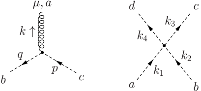
Figure A.1: Momentum routing for the tree level ghost-gluon and four-ghost vertices.

A.3.3 The four-ghost vertex

The bare four-ghost vertex $\Gamma_{4gh}^{(0)abcd}$ is derived from the four-ghost part of the action,

$$\mathcal{S}_{4gh}=\int d^{4}x^{\prime}\left\{\frac{\alpha}{2}\left(1-\frac{\alpha}{2}\right)\frac{\lambda}{2}g^{2}f^{ace}f^{bde}\bar{c}^{a}\bar{c}^{b}c^{c}c^{d}\right\}\,.$$ (A.25)

One obtains

$$\Gamma_{4gh}^{(0)abcd}(x,y,z,w) = \frac{\delta^{4}\mathcal{S}_{4gh}}{\delta\bar{c}^{a}(x)\delta\bar{c}^{b}(y)\delta c^{c}(z)\delta c^{d}(w)}$$ (A.26)

$$= \frac{\alpha}{2}\left(1-\frac{\alpha}{2}\right)\lambda g^{2}f^{abe}f^{cde}\delta^{4}(x-y)\delta^{4}(y-z)\delta^{4}(z-w).$$

With the momentum conventions given in Fig. A.1 the Fourier transformed bare four-ghost vertex is given by

$$\Gamma_{4gh}^{(0)abcd}(k_{1},k_{2},k_{3},k_{4}) = \frac{\alpha}{2}\left(1-\frac{\alpha}{2}\right)\lambda g^{2}f^{abe}f^{cde}(2\pi)^{4}\delta^{4}(k_{1}+k_{2}-k_{3}-k_{4}).$$ (A.27)

Again we define a reduced vertex function $\Gamma_{4gh}^{(0)}$ for convenience:

$$\Gamma_{4gh}^{(0)abcd}(k_{1},k_{2},k_{3},k_{4}) = g^{2}f^{abe}f^{cde}(2\pi)^{4}\delta^{4}(k_{1}+k_{2}-k_{3}-k_{4})\Gamma_{4g}^{(0)}$$

$$\Gamma_{4gh}^{(0)} = \frac{\alpha}{2}\left(1-\frac{\alpha}{2}\right)\lambda.$$ (A.28)

The full four-ghost vertex in coordinate space is formally given by

$$\Gamma^{abcd}(x,y,z)=\frac{\delta^{4}\Gamma}{\delta\bar{c}^{a}(x)\delta\bar{c}^{b}(y)\delta{c}^{c}(z)\delta{c}^{d}(y)}.$$ (A.29)

A.3.4 The other vertices

The quark-gluon vertex, the three-gluon vertex and the four-gluon vertex do not show up in the derivation of the ghost Dyson-Schwinger equation in appendix B. We therefore refrain from giving the expressions for these vertices in coordinate space but merely state the corresponding expressions for the bare vertices in momentum space. All vertices given in this subsection are reduced vertices i.e. we have suppressed a factor $(2\pi)^{4}$ and a delta function for momentum conservation.

The bare quark-gluon vertex in momentum space is given by

$$\Gamma^{(0)a}_{\mu}(k,q)=igt^{a}\gamma_{\mu}\,,$$ (A.30)

where $t^{a}$ is a generator of $SU(N_{c})$ gauge transformations.

For the bare three-gluon vertex in momentum space one finds

$$\Gamma^{(0)abc}_{\mu\nu\rho}(p,q,k)=gf^{abc}\left(\delta_{\mu\nu}\,(p-q)_{\rho}+\delta_{\nu\rho}\,(q-k)_{\mu}+\delta_{\rho\mu}\,(k-p)_{\nu}\right)\,,$$ (A.31)

where $f^{abc}$ is the structure constant of the gauge group. The three-gluon vertex is completely symmetric with respect to the three gluon momenta.

The four-gluon vertex is given by

$$\Gamma^{(0)abcd}_{\mu\nu\alpha\beta}(k_{1},k_{2},k_{3},k_{4}) = g^{2}\left\{f^{eab}f^{ecd}[\delta_{\mu\alpha}\,\delta_{\nu\beta}-\delta_{\mu\beta}\,\delta_{\nu\alpha}]+f^{ebc}f^{ead}[\delta_{\mu\nu}\,\delta_{\alpha\beta}-\delta_{\mu\alpha}\,\delta_{\nu\beta}]\right.$$ (A.32)

$$\left.\hskip 8.53581pt+f^{ebd}f^{eac}[\delta_{\mu\nu}\,\delta_{\alpha\beta}-\delta_{\nu\alpha}\,\delta_{\mu\beta}]\right\}\,,$$

and is symmetric in the Lorentz indices of the four attached gluons.

A.3.5 Decomposition of the connected ghost-gluon correlation function

For the derivation of the ghost Dyson-Schwinger equation from the generalised Lagrangian (2.11) performed in appendix B we will need some decompositions of connected correlation functions. These decompositions are derived in this and the next subsection. We will use the generating functional of connected Green’s functions, $W$, and the effective action, $\Gamma$, see appendix B for details. Furthermore we will exploit the fact that the fields and sources can be written as functional derivatives of $W$ and $\Gamma$:

$$\frac{\delta W}{\delta\sigma} = \bar{c},\hskip 28.45274pt\frac{\delta W}{\delta\bar{\sigma}}=c,\hskip 28.45274pt\frac{\delta W}{\delta J_{\mu}}=A_{\mu},$$

$$\frac{\delta\Gamma}{\delta c} = \bar{\sigma},\hskip 28.45274pt\frac{\delta\Gamma}{\delta\bar{c}}=\bar{\sigma},\hskip 28.45274pt\frac{\delta\Gamma}{\delta A_{\mu}}=J_{\mu}.$$ (A.33)

The sign conventions have been chosen such that derivatives with respect to $\bar{c}$ and $\bar{\sigma}$ are left derivatives whereas the ones with respect to ${c}$ and ${\sigma}$ are right derivatives.

With the help of the matrix relation

$$\frac{\delta\chi^{-1}}{\delta\phi}=-\chi^{-1}\frac{\delta\chi}{\delta\phi}\chi^{-1},$$ (A.34)

and the identity

$$\delta(y-x)\delta^{ab}=\int d^{4}z\frac{\delta\bar{\sigma}^{b}(y)}{\delta\bar{c}^{d}(z)}\frac{\delta\bar{c}^{d}(z)}{\delta\bar{\sigma}^{a}(x)} = \int d^{4}z\frac{\delta^{2}\Gamma}{\delta\bar{c}^{d}(z)\delta c^{b}(y)}\frac{\delta^{2}W}{\delta\bar{\sigma}^{a}(x)\delta\sigma^{d}(z)}\,,$$ (A.35)

we decompose the connected ghost-gluon correlation function, $\langle A^{a}_{\mu}(x)\bar{c}^{b}(y)c^{c}(z)\rangle$, in the following way:

$$\langle A^{a}_{\mu}(x)\bar{c}^{b}(y)c^{c}(z)\rangle = \frac{\delta^{3}W}{\delta J^{a}_{\mu}(x)\delta\bar{\sigma}^{b}(y)\delta{\sigma}^{c}(z)}$$ (A.36)

$$=\frac{\delta}{\delta J^{a}_{\mu}(x)}\left[\frac{\delta^{2}\Gamma}{\delta\bar{c}^{b}(y)\delta{c}^{c}(z)}\right]^{-1}$$

$$=\int d^{4}u_{1}\frac{\delta A^{d}_{\nu}(u_{1})}{\delta J^{a}_{\mu}(x)}\frac{\delta}{\delta A^{d}_{\nu}(u_{1})}\left[\frac{\delta^{2}\Gamma}{\delta\bar{c}^{b}(y)\delta{c}^{c}(z)}\right]^{-1}$$

$$=\int d^{4}[u_{1}u_{2}u_{3}]\frac{\delta^{2}W}{\delta J^{a}_{\mu}(x)\delta J^{d}_{\nu}(u_{1})}\>\frac{\delta^{2}W}{\delta\bar{\sigma}^{b}(y)\delta{\sigma}^{e}(u_{2})}\>\frac{\delta^{3}\Gamma}{\delta A^{d}_{\nu}(u_{1})\delta\bar{c}^{e}(u_{2})\delta{c}^{f}(u_{3})}\>\frac{\delta^{2}W}{\delta\bar{\sigma}^{f}(u_{3})\delta{\sigma}^{c}(z)}$$

$$=\int d^{4}[u_{1}u_{2}u_{3}]D_{\mu\nu}^{ad}(x-u_{1})D_{G}^{eb}(u_{2}-y)\Gamma^{def}_{\nu}(u_{1},u_{2},u_{3})D_{G}^{cf}(u_{3}-z).$$

Here we used the abbreviation $d^{4}[u_{1}u_{2}u_{3}]:=d^{4}u_{1}\,d^{4}u_{2}\,d^{4}u_{3}$ and the definitions of the gluon propagator $D_{\mu\nu}$, the ghost propagator $D_{G}$ and the ghost-gluon vertex $\Gamma_{\nu}$ given in previous subsections.

A.3.6 Decomposition of connected four-ghost correlation function

Furthermore we need the decomposition of the four-ghost correlation function into one-particle irreducible parts. We start at a stage where the sources are still present and set them to zero at the end of the derivation. We first give the decomposition of the connected ghost-antighost-ghost three-point function

$$\langle\bar{c}^{b}(y){c}^{c}(z)\bar{c}^{d}(w)\rangle = \frac{\delta^{3}W}{\delta\bar{\sigma}^{b}(y)\delta\sigma^{c}(z)\delta\bar{\sigma}^{d}(w)}$$

$$=\frac{\delta}{\delta\bar{\sigma}^{b}(y)}\left[\frac{\delta^{2}\Gamma}{\delta\sigma^{c}(z)\delta\bar{\sigma}^{d}(w)}\right]^{-1}$$

$$=\int d^{4}u_{1}\frac{\delta A^{e}_{\nu}(u_{1})}{\delta\bar{\sigma}^{b}(y)}\frac{\delta}{\delta A^{e}_{\nu}(u_{1})}\left[\frac{\delta^{2}\Gamma}{\delta\sigma^{c}(z)\delta\bar{\sigma}^{d}(w)}\right]^{-1}$$

$$=\int d^{4}[u_{1}u_{2}u_{3}]\frac{\delta^{2}W}{\delta\bar{\sigma}^{b}(y)\delta J^{e}_{\nu}(u_{1})}\>\frac{\delta^{2}W}{\delta\sigma^{c}(z)\delta\bar{\sigma}^{f}(u_{2})}\>\frac{\delta^{3}\Gamma}{\delta A^{e}_{\nu}(u_{1})\delta{c}^{f}(u_{2})\delta\bar{c}^{g}(u_{3})}\>\frac{\delta^{2}W}{\delta\sigma^{g}(u_{3})\delta\bar{\sigma}^{d}(w)}\,.$$

Then we decompose the connected four-ghost Green’s function:

$$\langle{c}^{a}(x)\bar{c}^{b}(y){c}^{c}(z)\bar{c}^{d}(w)\rangle = \frac{\delta^{4}W}{\delta\sigma^{a}(x)\delta\bar{\sigma}^{b}(y)\delta\sigma^{c}(z)\delta\bar{\sigma}^{d}(w)}$$ (A.38)

$$= \frac{\delta}{\delta\sigma^{a}(x)}\int d^{4}[u_{1}u_{2}u_{3}]\frac{\delta^{2}W}{\delta\bar{\sigma}^{b}(y)\delta J^{e}_{\mu}(u_{1})}\>\frac{\delta^{2}W}{\delta\sigma^{c}(z)\delta\bar{\sigma}^{f}(u_{2})}$$

$$\hskip 42.67912pt\times\frac{\delta^{3}\Gamma}{\delta A^{e}_{\mu}(u_{1})\delta{c}^{f}(u_{2})\delta\bar{c}^{g}(u_{3})}\>\frac{\delta^{2}W}{\delta\sigma^{g}(u_{3})\delta\bar{\sigma}^{d}(w)}.\hskip 28.45274pt$$

Carrying out the remaining derivative gives four terms. The two terms where the derivative acts on the second and on the last propagator vanish, because the term $\frac{\delta W}{\delta\bar{\sigma}^{b}(y)\delta J^{e}_{\nu}(u_{1})}$ vanishes when the sources are set to zero. The contribution where the derivative acts on the first propagator can be treated using eq. (A.36). In the expression with the derivative acting on the vertex we use

$$-\frac{\delta^{2}W}{\delta\bar{\sigma}^{b}(y)\delta J^{e}_{\mu}(u_{1})}\frac{\delta^{4}\Gamma}{\delta\sigma^{a}(x)\delta A^{e}_{\mu}(u_{1})\delta{c}^{f}(u_{2})\delta\bar{c}^{g}(u_{3})} = \frac{\delta^{4}\Gamma}{\delta\sigma^{a}(x)\delta\bar{\sigma}^{b}(y)\delta{c}^{f}(u_{2})\delta\bar{c}^{g}(u_{3})}$$

$$=\int d^{4}u_{4}\frac{\delta^{2}W}{\delta\sigma^{a}(x)\bar{\sigma}^{e}(u_{4})}\>\>\frac{\delta^{4}\Gamma}{\delta c^{e}(u_{4})\delta\bar{\sigma}^{b}(y)\delta{c}^{f}(u_{2})\delta\bar{c}^{g}(u_{3})}$$

$$=\int d^{4}[u_{4}u_{5}]\frac{\delta^{2}W}{\delta\sigma^{a}(x)\bar{\sigma}^{e}(u_{4})}\>\>\frac{\delta^{2}W}{\delta\bar{\sigma}^{b}(y)\delta{\sigma}^{h}(u_{5})}\>\>\frac{\delta^{4}\Gamma}{\delta c^{e}(u_{4})\delta\bar{c}^{h}(u_{5})\delta{c}^{f}(u_{2})\delta\bar{c}^{g}(u_{3})}$$

$$=-\int d^{4}[u_{4}u_{5}]\frac{\delta^{2}W}{\delta\sigma^{a}(x)\bar{\sigma}^{e}(u_{4})}\>\>\frac{\delta^{2}W}{\delta{\sigma}^{h}(u_{5})\delta\bar{\sigma}^{b}(y)}\>\>\frac{\delta^{4}\Gamma}{\delta\bar{c}^{g}(u_{3})\delta\bar{c}^{h}(u_{5})\delta c^{e}(u_{4})\delta{c}^{f}(u_{2})}.$$

Collecting all this together we arrive at

$$\langle{c}^{a}(x)\bar{c}^{b}(y){c}^{c}(z)\bar{c}^{d}(w)\rangle = \int d^{4}[u_{1}u_{2}u_{3}u_{4}u_{5}u_{6}]\left\{\frac{\delta^{2}W}{\delta J^{e}_{\mu}(u_{1})\delta J^{f}_{\nu}(u_{4})}\>\>\frac{\delta^{2}W}{\delta\sigma^{a}(x)\delta\bar{\sigma}^{g}(u_{5})}\right.$$ (A.40)

$$\hskip 28.45274pt\times\frac{\delta^{3}\Gamma}{\delta A^{f}_{\nu}(u_{4})\delta{c}^{g}(u_{5})\delta\bar{c}^{h}(u_{6})}\>\>\frac{\delta^{2}W}{\delta\sigma^{h}(u_{6})\delta\bar{\sigma}^{b}(y)}\>\>\frac{\delta^{2}W}{\delta\sigma^{c}(z)\delta\bar{\sigma}^{i}(u_{2})}$$

$$\hskip 28.45274pt\left.\times\frac{\delta^{3}\Gamma}{\delta A^{e}_{\mu}(u_{1})\delta{c}^{i}(u_{2})\delta\bar{c}^{j}(u_{3})}\>\>\frac{\delta^{2}W}{\delta\sigma^{j}(u_{3})\delta\bar{\sigma}^{d}(w)}\right\}$$

$$- \int d^{4}[u_{1}u_{2}u_{3}u_{4}u_{5}]\left\{\frac{\delta^{2}W}{\delta\sigma^{a}(x)\bar{\sigma}^{e}(u_{4})}\>\>\frac{\delta^{2}W}{\delta{\sigma}^{h}(u_{5})\delta\bar{\sigma}^{b}(y)}\right.$$

$$\hskip 28.45274pt\times\frac{\delta^{2}W}{\delta\sigma^{c}(z)\delta\bar{\sigma}^{f}(u_{2})}\>\>\frac{\delta^{4}\Gamma}{\delta\bar{c}^{g}(u_{3})\delta\bar{c}^{h}(u_{5})\delta c^{e}(u_{4})\delta{c}^{f}(u_{2})}$$

$$\hskip 28.45274pt\times\left.\frac{\delta^{2}W}{\delta\sigma^{g}(u_{3})\delta\bar{\sigma}^{d}(w)}\right\}.$$

Interchanging some Grassmann fields in the correlations and using the definitions for the propagators and vertices given in the previous subsections we arrive at

$$\langle\bar{c}^{b}(y)\bar{c}^{d}(w){c}^{a}(x){c}^{c}(z)\rangle = \int d^{4}[u_{1}u_{2}u_{3}u_{4}u_{5}u_{6}]\left\{D_{\mu\nu}^{ef}(u_{1}-u_{4})\,D_{G}^{ag}(x-u_{5})\right.$$ (A.41)

$$\hskip 28.45274pt\times\Gamma^{fhg}_{\nu}(u_{4},u_{6},u_{5})D_{G}^{hb}(u_{6}-y)\,D_{G}^{ci}(z-u_{2})$$

$$\hskip 28.45274pt\left.\times\Gamma^{eji}_{\mu}(u_{1},u_{3},u_{2})\,D_{G}^{jd}(u_{3}-w)\right\}$$

$$+ \int d^{4}[u_{1}u_{2}u_{3}u_{4}u_{5}]\left\{D_{G}^{ae}(x-u_{4})\,D_{G}^{hb}(u_{5}-y)\right.$$

$$\hskip 28.45274pt\left.\times D_{G}^{cf}(z-u_{2})\,\Gamma_{4gh}^{hgef}(u_{5},u_{3},u_{4},u_{2})\,D_{G}^{gd}(u_{3}-w)\right\},\hskip 28.45274pt$$

which is the decomposition of the four-ghost correlation used in appendix B.

Appendix B The derivation of the ghost Dyson-Schwinger equation in general ghost-antighost symmetric gauges

In this appendix we will derive the ghost Dyson-Schwinger equation from the generalised Lagrangian (2.11). As there are no direct couplings between quarks and ghosts contained in the Lagrangian it is sufficient to employ only the ghost-gluon part. We start by transforming the ghost-gluon part of the Lagrangian into a more suitable form using partial integrations under the assumption of vanishing fields at infinity. We obtain

$$\cal{L} = \frac{1}{2}A_{\mu}^{a}\left(-\partial^{2}\delta_{\mu\nu}+\left(1-\frac{1}{\lambda}\right)\partial_{\mu}\partial_{\nu}\right)A_{\nu}^{a}-gf^{abc}\left(\partial_{\mu}A_{\nu}^{a}\right)A_{\mu}^{b}A_{\nu}^{c}$$ (B.1)

$$+\frac{g^{2}}{4}f^{abe}f^{cde}A_{\mu}^{a}A_{\nu}^{b}A_{\mu}^{c}A_{\nu}^{d}+\bar{c}^{a}\partial^{2}c^{a}+\frac{\alpha}{2}\left(1-\frac{\alpha}{2}\right)\frac{\lambda}{2}g^{2}f^{ace}f^{bde}\bar{c}^{a}\bar{c}^{b}c^{c}c^{d}$$

$$+i\left(1-\frac{\alpha}{2}\right)gf^{abc}\bar{c}^{a}\partial_{\mu}\left(A_{\mu}^{c}c^{b}\right)+i\frac{\alpha}{2}gf^{abc}\bar{c}^{a}A_{\mu}^{c}\partial_{\mu}c^{b}.$$

The partition function of the theory is given by

$$Z[J,\sigma,\bar{\sigma}]=\int{\cal D}[A\bar{c}c]\exp\left\{-\int d^{4}z\,{\cal{L}}+\int d^{4}z\,\left(A^{a}J^{a}+\bar{\sigma}c+\bar{c}\sigma\right)\right\}$$ (B.2)

with the sources $J$, $\sigma$ and $\bar{\sigma}$ of the gluon, antighost and ghost fields, respectively. The action is given by $\mathcal{S}[J,c,\bar{c}]=\int d^{4}z\,{\cal{L}}$. The generating functional of connected Green’s functions, $W[J,\sigma,\bar{\sigma}]$, is defined as the logarithm of the partition function. The functional Legendre transform of $W$ is the effective action

$$\Gamma[A,\bar{c},c]=-W[J,\sigma,\bar{\sigma}]+\int d^{4}z\left(A^{a}J^{a}+\bar{\sigma}c+\bar{c}\sigma\right),$$ (B.3)

which is the generating functional of one-particle irreducible vertex functions. The fields and sources can be written as functional derivatives of the respective generating functionals in the following way

$$\frac{\delta W}{\delta\sigma} = \bar{c},\hskip 28.45274pt\frac{\delta W}{\delta\bar{\sigma}}=c,\hskip 28.45274pt\frac{\delta W}{\delta J_{\mu}}=A_{\mu},$$

$$\frac{\delta\Gamma}{\delta c} = \bar{\sigma},\hskip 28.45274pt\frac{\delta\Gamma}{\delta\bar{c}}=\bar{\sigma},\hskip 28.45274pt\frac{\delta\Gamma}{\delta A_{\mu}}=J_{\mu}.$$ (B.4)

The sign conventions have been chosen such that derivatives with respect to $\bar{c}$ and $\bar{\sigma}$ are left derivatives whereas the ones with respect to ${c}$ and ${\sigma}$ are right derivatives,

$$\frac{\delta}{\delta\left(\bar{\sigma},\bar{c}\right)}:=\mbox{left derivative}\hskip 28.45274pt\frac{\delta}{\delta\left({\sigma},{c}\right)}:=\mbox{right derivative}.$$ (B.5)

Given that the functional integral is well-defined, the Dyson-Schwinger equation for the ghost propagator is derived from the observation that the integral of a total derivative vanishes. We take the derivative with respect to the antighost field and obtain

$$0 = \int{\cal D}[A\bar{c}c]\frac{\delta}{\delta\bar{c}}\exp\left\{-\int d^{4}z\,{\cal{L}}+\int d^{4}z\,\left(A^{a}J^{a}+\bar{\sigma}c+\bar{c}\sigma\right)\right\}$$ (B.6)

$$= \int{\cal D}[A\bar{c}c]\left(-\frac{\delta S\left[A,c,\bar{c}\right]}{\delta\bar{c}}+\sigma\right)\exp\left\{-\int d^{4}z\,{\cal{L}}+\int d^{4}z\,\left(A^{a}J^{a}+\bar{\sigma}c+\bar{c}\sigma\right)\right\}$$

$$= \left(-\frac{\delta S\left[\frac{\delta}{\delta J},\frac{\delta}{\delta\bar{\sigma}},\frac{\delta}{\delta\sigma}\right]}{\delta\bar{c}}+\sigma\right)Z[J,\sigma,\bar{\sigma}].$$

Now we use the relations (B.4) and apply a further functional derivative with respect to the source $\sigma^{b}(y)$. We arrive at

$$0=\left(-\frac{\delta S}{\delta\bar{c}^{c}(z)}\bar{c}^{b}(y)+\sigma^{c}(z)\bar{c}^{b}(y)+\delta(z-y)\delta_{cb}\right)Z[J,\sigma,\bar{\sigma}]$$ (B.7)

with explicit colour indices and space-time arguments. Setting the sources equal to zero we obtain the ghost Dyson-Schwinger equation

$$\left\langle\frac{\delta S}{\delta\bar{c}^{c}(z)}\bar{c}^{b}(y)\right\rangle=\delta(z-y)\delta_{cb}.$$ (B.8)

The derivative is easily calculated

$$\frac{\delta S}{\delta\bar{c}^{c}(z)} = \partial^{2}c^{c}(z)+\frac{\alpha}{2}\left(1-\frac{\alpha}{2}\right)\frac{\lambda}{2}g^{2}f^{cde}f^{fge}\bar{c}^{d}(z)c^{f}(z)c^{g}(z)$$ (B.9)

$$+i\left(1-\frac{\alpha}{2}\right)gf^{cde}\partial_{\mu}\left(A^{e}_{\mu}(z)c^{d}(z)\right)+i\frac{\alpha}{2}gf^{cde}A^{e}_{\mu}(z)\partial_{\mu}c^{d}(z).$$

Whereas in the covariant formalism full and connected three-point functions are the same, the four-point correlations have to be decomposed into disconnected and connected parts. For the four-ghost correlation function this results in

$$\langle\bar{c}^{b}(y)\bar{c}^{d}(z)c^{f}(z)c^{g}(z)\rangle = \langle\bar{c}^{b}(y)c^{g}(z)\rangle\,\langle\bar{c}^{d}(z)c^{f}(z)\rangle-\langle\bar{c}^{b}(y)c^{f}(z)\rangle\,\langle\bar{c}^{d}(z)c^{g}(z)\rangle$$ (B.10)

$$+ \langle\bar{c}^{b}(y)\bar{c}^{d}(z)c^{f}(z)c^{g}(z)\rangle_{conn.}\,.$$

Keeping in mind the Grassmann nature of the ghost and antighost fields we then obtain

$$-\delta(z-y)\delta_{cb} = \partial^{2}\langle\bar{c}^{b}(y)c^{c}(z)\rangle+\frac{\alpha}{2}\left(1-\frac{\alpha}{2}\right)\frac{\lambda}{2}g^{2}f^{cde}f^{fge}\left\{\langle\bar{c}^{b}(y)\bar{c}^{d}(z)c^{f}(z)c^{g}(z)\rangle\right.$$

$$\left.+\left(\langle\bar{c}^{b}(y)c^{g}(z)\rangle\,\langle\bar{c}^{d}(z)c^{f}(z)\rangle-\langle\bar{c}^{b}(y)c^{f}(z)\rangle\,\langle\bar{c}^{d}(z)c^{g}(z)\rangle\right)\right\}$$

$$+ \left(1-\frac{\alpha}{2}\right)gf^{cde}\langle\bar{c}^{b}(y)\partial_{\mu}\left(A^{e}_{\mu}(z)c^{d}(z)\right)\rangle+\frac{\alpha}{2}gf^{cde}\langle\bar{c}^{b}(y)A^{e}_{\mu}(z)\partial_{\mu}c^{d}(z)\rangle\,,$$

where all correlations are connected Green’s functions. We now use the relation

$$\delta(y-x)\delta^{ab}=\frac{\delta\bar{\sigma}^{b}(y)}{\delta\bar{\sigma}^{a}(x)}=\int d^{4}z\frac{\delta\bar{\sigma}^{b}(y)}{\delta\bar{c}^{d}(z)}\frac{\delta\bar{c}^{d}(z)}{\delta\bar{\sigma}^{a}(x)} = \int d^{4}z\frac{\delta^{2}\Gamma}{\delta\bar{c}^{d}(z)\delta c^{b}(y)}\frac{\delta^{2}W}{\delta\bar{\sigma}^{a}(x)\delta\sigma^{d}(z)}$$

$$=: \int d^{4}z\left[D_{G}^{db}(z-y)\right]^{-1}D_{G}^{ad}(x-z)$$

and multiply eq. (LABEL:DSEa) with $-[D_{G}^{ac}(x-z)]^{-1}=\left[\langle\bar{c}^{c}(z)c^{a}(x)\rangle\right]^{-1}$. We arrive at

$$[D_{G}^{ab}(x-y)]^{-1} = \partial^{2}\delta(x-y)\delta^{ab}$$

$$- \frac{\alpha}{2}\left(1-\frac{\alpha}{2}\right)\frac{\lambda}{2}g^{2}f^{cde}f^{fge}\int d^{4}z\,[D_{G}^{ac}(x-z)]^{-1}\left\{\langle\bar{c}^{b}(y)\bar{c}^{d}(z)c^{f}(z)c^{g}(z)\rangle\right.$$

$$\hskip 68.28644pt+\,\left.\langle\bar{c}^{b}(y)c^{g}(z)\rangle\,\langle\bar{c}^{d}(z)c^{f}(z)\rangle-\langle\bar{c}^{b}(y)c^{f}(z)\rangle\,\langle\bar{c}^{d}(z)c^{g}(z)\rangle\right\}$$

$$- i\left(1-\frac{\alpha}{2}\right)gf^{cde}\int d^{4}z\,[D_{G}^{ac}(x-z)]^{-1}\langle\bar{c}^{b}(y)\partial_{\mu}\left(A^{e}_{\mu}(z)c^{d}(z)\right)\rangle$$

$$- i\frac{\alpha}{2}gf^{cde}\int d^{4}z\,[D_{G}^{ac}(x-z)]^{-1}\langle\bar{c}^{b}(y)A^{e}_{\mu}(z)\partial_{\mu}c^{d}(z)\rangle.$$

Before we decompose the connected Green’s functions into one particle irreducible ones we have to take care of the space-time derivatives. Noting that

$$\partial_{\mu}^{z}\frac{\delta^{2}W}{\delta J^{c}_{\mu}(z)\sigma^{d}(z)} = -\int d^{4}u\partial_{\mu}^{u}\left(\delta(u-z)\right)\frac{\delta^{2}W}{\delta J^{c}_{\mu}(u)\sigma^{d}(u)}$$ (B.14)

$$= -\int d^{4}[uv]\partial_{\mu}^{u}\left(\delta(u-z)\right)\delta(u-v)\frac{\delta^{2}W}{\delta J^{c}_{\mu}(v)\sigma^{d}(u)}$$

with the abbreviation $d^{4}u\,d^{4}v=:d^{4}[uv]$, and

$$\frac{\delta}{\delta J^{c}_{\mu}(z)}\partial_{\mu}^{z}\frac{\delta W}{\sigma^{d}(z)} = \int d^{4}[uv]\,\delta(u-z)\delta(u-v)\frac{\delta}{\delta J^{c}_{\mu}(v)}\partial_{\mu}^{u}\frac{\delta W}{\sigma^{d}(u)}$$ (B.15)

$$= -\int d^{4}[uv]\,\partial_{\mu}^{u}\left(\delta(u-z)\delta(u-v)\right)\frac{\delta^{2}W}{\delta J^{c}_{\mu}(v)\sigma^{d}(u)}$$

we can replace the derivative terms by the bare ghost-gluon vertex defined in appendix A.3. The tadpole term can be treated in the following way:

$$\int d^{4}z[D_{G}^{ac}(x-z)]^{-1}f^{cde}f^{fge}\left\{\langle\bar{c}^{b}(y)c^{g}(z)\rangle\,\langle\bar{c}^{d}(z)c^{f}(z)\rangle-\langle\bar{c}^{b}(y)c^{f}(z)\rangle\,\langle\bar{c}^{d}(z)c^{g}(z)\rangle\right\}$$ (B.16)

$$=2\int d^{4}z\,[D_{G}^{ac}(x-z)]^{-1}f^{cde}f^{fge}\left\{\langle\bar{c}^{b}(y)c^{g}(z)\rangle\,\langle\bar{c}^{d}(z)c^{f}(z)\rangle\right\}$$

$$=2\int d^{4}[zuv]\,[D_{G}^{ac}(x-z)]^{-1}\delta(z-u)\,\delta(u-v)\,f^{cde}f^{fge}\,D_{G}^{gb}(z-y)\,D_{G}^{fd}(v-u)$$

$$=2\int d^{4}[uv]\,\delta(x-y)\,\delta(z-u)\,\delta(u-v)\,f^{bde}f^{fae}\,D_{G}^{fd}(v-u).$$

Plugging the expressions for the ghost-gluon loop and the one for the tadpole into eq. (LABEL:DSEb) and using the expression for the bare four-ghost vertex given in appendix A.3 we obtain

$$[D_{G}^{ab}(x-y)]^{-1} = \partial^{2}\delta(x-y)\delta^{ab}-\int d^{4}[uv]\,\Gamma_{4gh}^{(0)bdfa}(x,u,v,y)\,D_{G}^{fd}(v-u)$$

$$+\frac{\alpha}{2}\left(1-\frac{\alpha}{2}\right)\frac{\lambda}{2}g^{2}f^{cde}f^{fge}\times$$

$$\hskip 14.22636pt\int d^{4}[zuv]\,\delta(z-u)\,\delta(u-v)\,[D_{G}^{ac}(x-z)]^{-1}\>\langle\bar{c}^{b}(y)\bar{c}^{d}(z)c^{f}(u)c^{g}(v)\rangle$$

$$-\int d^{4}[zuv]\,\Gamma^{(0)cde}_{\mu}(z,u,v)\,[D_{G}^{ac}(x-z)]^{-1}\,\langle\bar{c}^{b}(y)A^{e}_{\mu}(v)c^{d}(u)\rangle\,.$$

To decompose the connected Green’s functions into one-particle irreducible ones we use the relations

$$\langle A^{e}_{\mu}(v)\bar{c}^{b}(y)c^{d}(u)\rangle = \int d^{4}[z_{1}z_{2}z_{3}]\,D_{\mu\nu}^{ef}(v-z_{1})\,D_{G}^{bg}(y-z_{2})\,\Gamma_{\nu}^{fhg}(z_{1},z_{3},z_{2})\,D_{G}^{hd}(u-z_{3})$$

$$\langle\bar{c}^{b}(y)\bar{c}^{d}(z)c^{f}(u)c^{g}(v)\rangle = \int d^{4}[u_{1}u_{2}u_{3}u_{4}u_{5}u_{6}]\,\left\{D_{\mu\nu}^{ek}(u_{1}-u_{4})\,D_{G}^{fl}(u-u_{5})\right.$$ (B.19)

$$\hskip 28.45274pt\times\,\Gamma^{khl}_{\nu}(u_{4},u_{6},u_{5})\,D_{G}^{hb}(u_{6}-y)\,D_{G}^{gi}(v-u_{2})$$

$$\hskip 28.45274pt\left.\times\,\Gamma^{eji}_{\mu}(u_{1},u_{3},u_{2})\,D_{G}^{jd}(u_{3}-z)\right\}$$

$$- \int d^{4}[u_{1}u_{2}u_{3}u_{4}u_{5}]\,\left\{D_{G}^{fe}(u-u_{4})\,D_{G}^{hb}(u_{5}-y)\right.$$

$$\hskip 28.45274pt\left.\times\,D_{G}^{gi}(v-u_{2})\,\Gamma_{4gh}^{jhei}(u_{3},u_{5},u_{4},u_{2})\,D_{G}^{jd}(u_{3}-z)\right\}\,,\hskip 42.67912pt$$

which have been derived in appendix A.3.

Substituting these expressions into eq. (LABEL:DSEd) we arrive at the final expression for the ghost Dyson-Schwinger equation in coordinate space:

$$[D_{G}^{ab}(x-y)]^{-1} = [D_{G}^{(0)ab}(x-y)]^{-1}$$

$$- \int d^{4}[uv]\,\Gamma_{4gh}^{(0)bdfa}(x,u,v,y)\,D_{G}^{fd}(v-u)$$

$$- \frac{1}{2}\int d^{4}[zuvu_{1}u_{2}u_{3}u_{4}u_{5}]\,\Gamma^{(0)bdgf}_{4gh}(y,z,v,u)\,D_{\mu\nu}^{ek}(u_{1}-u_{4})\,D_{G}^{fl}(u-u_{5})$$

$$\hskip 28.45274pt\times\,\Gamma^{kal}_{\nu}(u_{4},x,u_{5})\,D_{G}^{gi}(v-u_{2})\,\Gamma^{eij}_{\mu}(u_{1},u_{3},u_{2})\,D_{G}^{jd}(u_{3}-z)$$

$$- \frac{1}{2}\int d^{4}[zuvu_{1}u_{2}u_{3}u_{4}]\Gamma^{(0)bdgf}_{4gh}(y,z,v,u)\,D_{G}^{fe}(u-u_{4})$$

$$\hskip 28.45274pt\times\,D_{G}^{gi}(v-u_{2})\,\Gamma_{4gh}^{jaei}(u_{3},x,u_{4},u_{2})\,D_{G}^{jd}(u_{3}-z)$$

$$- \int d^{4}[zuvz_{1}z_{2}z_{3}]\,\Gamma^{(0)bde}_{\mu}(y,u,v)\,D_{\mu\nu}^{ef}(v-z_{1})\,\Gamma_{\nu}^{fha}(z_{1},z_{3},x)D_{G}^{hd}(u-z_{3})$$

where an additional minus signs arises from the interchange of the colour indices $f$ and $g$ in the bare four-ghost vertices and from the interchange of $j$ and $i$ in the ghost-gluon vertex.

After performing a Fourier transformation we obtain the respective expression in momentum space

$$[D_{G}(p)]^{-1} = [D_{G}^{(0)}(p)]^{-1}$$

$$+ \left(-N_{c}\right)\frac{g^{2}}{(2\pi)^{4}}\int d^{4}q\>\Gamma_{4gh}^{(0)}\>D_{G}(q)$$

$$+ \left(\frac{-N_{c}^{2}}{2}\right)\frac{1}{2}\frac{g^{4}}{(2\pi)^{8}}\int d^{4}[q_{1}q_{2}]\>\Gamma^{(0)}_{4gh}\>D_{\mu\nu}(p-q_{1})\>D_{G}(q1)$$

$$\hskip 28.45274pt\times\,\Gamma_{\nu}(p,q_{1})\>D_{G}(q_{2})\>\Gamma_{\mu}(-p+q_{1}+q_{2},q_{2})\>D_{G}(p-q_{1}-q_{2})$$

$$- \left(-N_{c}^{2}\right)\frac{1}{2}\frac{g^{4}}{(2\pi)^{8}}\int d^{4}[q_{1}q_{2}]\Gamma^{(0)}_{4gh}\>D_{G}(q_{1})\>D_{G}(p-q_{1}-q_{2})\>\Gamma_{4gh}(p,q_{1},q_{2})\>D_{G}(q_{2})$$

$$+ \left(-N_{c}\right)\frac{g^{2}}{(2\pi)^{4}}\int d^{4}q\>\Gamma^{(0)}_{\mu}(p,q)\>D_{\mu\nu}(p-q)\>\Gamma_{\nu}(q,p)D_{G}(q)$$

where the colour traces have been carried out and the reduced vertices defined in appendix A.3 have been used.

Appendix C Methods to solve DSEs in flat Euclidean space-time

C.1 Angular integrals

Working in Euclidean space-time the four dimensional integrals in the loops of Dyson-Schwinger equations can be transformed to hyperspherical coordinates as

$$\int d^{4}q\>\ldots=\frac{1}{2}\int_{0}^{\infty}dq^{2}q^{2}\int_{0}^{2\pi}d\Phi\int_{0}^{\pi}d\Psi\sin(\Psi)\int_{0}^{\pi}d\theta\sin^{2}(\theta)\>\ldots.$$ (C.1)

We choose the external momentum $p_{\mu}$ to point in the four-direction, enclosing the angle $\theta$ with the loop momentum $q_{\mu}$. All integrands are then functions of the squared external momentum, the squared loop momentum and the angle $\theta$ only. The other two angular integrals can then be performed trivially yielding a factor of $4\pi$. We thus have the relation

$$\int d^{4}q\,f(p^{2},q^{2},\theta)=2\pi\int_{0}^{\infty}dq^{2}q^{2}\int_{0}^{\pi}d\theta\sin^{2}(\theta)\,f(p^{2},q^{2},\theta),$$ (C.2)

which is used frequently throughout this thesis.

Sometimes the remaining angular integral can be performed as well using the integration formulae

$$\int_{0}^{\pi}d\theta\frac{\sin^{2}(\theta)}{z^{2}} = \frac{\pi}{2}\left[\frac{\Theta(x-y)}{x(x-y)}+\frac{\Theta(y-x)}{y(y-x)}\right]$$ (C.3)

$$\int_{0}^{\pi}d\theta\frac{\sin^{2}(\theta)}{z} = \frac{\pi}{2}\left[\frac{\Theta(x-y)}{x}+\frac{\Theta(y-x)}{y}\right]$$ (C.4)

$$\int_{0}^{\pi}d\theta\sin^{2}(\theta) = \frac{\pi}{2}$$ (C.5)

$$\int_{0}^{\pi}d\theta\sin^{2}(\theta)\>z = \frac{\pi}{2}(x+y)$$ (C.6)

$$\int_{0}^{\pi}d\theta\sin^{2}(\theta)\>z^{2} = \frac{\pi}{2}\left((x+y)^{2}+xy\right)$$ (C.7)

where we have used the abbreviations $x:=p^{2}$, $y:=q^{2}$ and the squared momentum $z$ is defined as $z=(p-q)^{2}=x+y-2\sqrt{xy}\cos(\theta)$. A derivation of eqs. (C.3), (C.4) can be found e.g. in [141].

C.2 Tensor integrals

The explicit expression for the scalar bubble integral $I$, defined in eq. (C.8), can be easily evaluated in Euclidean space-time using the Feynman-parameterisation (see e.g. ref. [5]). With the squared momenta $x=p^{2}$, $y=q^{2}$ and $z=(p-q)^{2}$ the result is given by

$$I(a,b,p) := \int d^{4}q\frac{1}{y^{a}z^{b}}$$ (C.8)

$$= \pi^{2}\,x^{2-a-b}\,\frac{\Gamma(2-a)\,\Gamma(2-b)\,\Gamma(a+b-2)}{\Gamma(a)\,\Gamma(b)\,\Gamma(4-a-b)}\,.$$ (C.9)

The corresponding tensor integrals can be reduced to scalar integrals by extracting combinations of momenta $p_{\mu}$ and the symmetric tensor $\delta_{\mu\nu}$ according to the symmetry properties of the integrand:

$$J_{\mu}(a,b,p) := \int d^{4}q\frac{q_{\mu}}{y^{a}z^{b}}\hskip 19.91684pt=J_{1}(a,b,p)\,\,p_{\mu}\,,$$ (C.10)

$$K_{\mu\nu}(a,b,p) := \int d^{4}q\frac{q_{\mu}q_{\nu}}{y^{a}z^{b}}\hskip 17.07182pt\,=K_{1}(a,b,p)\,\,p_{\mu}p_{\nu}+K_{2}(a,b,p)\,\,x\,\delta_{\mu\nu}\,,$$ (C.11)

$$L_{\mu\nu\rho}(a,b,p) := \int d^{4}q\frac{q_{\mu}q_{\nu}q_{\rho}}{y^{a}z^{b}}\hskip 8.5359pt\,=L_{1}(a,b,p)\,\,p_{\mu}p_{\nu}p_{\rho}$$ (C.12)

$$\hskip 76.82234pt\,+\,L_{2}(a,b,p)\,\,x\,\left(p_{\mu}\,\delta_{\nu\rho}+p_{\nu}\,\delta_{\rho\mu}+p_{\rho}\,\delta_{\mu\nu}\right)\,,$$

$$M_{\mu\nu\rho\sigma}(a,b,p) := \int d^{4}q\frac{q_{\mu}q_{\nu}q_{\rho}q_{\sigma}}{y^{a}z^{b}}=M_{1}(a,b,p)\,\,p_{\mu}p_{\nu}p_{\rho}p_{\sigma}$$ (C.13)

$$\hskip 79.6678pt+\,M_{2}(a,b,p)\,\,x\,\left(\delta_{\mu\nu}\,p_{\rho}p_{\sigma}+\delta_{\mu\rho}\,p_{\nu}p_{\sigma}+\delta_{\mu\sigma}\,p_{\rho}p_{\mu}+\right.$$

$$\hskip 159.3356pt\left.\,\delta_{\nu\rho}\,p_{\mu}p_{\sigma}+\delta_{\nu\sigma}\,p_{\rho}p_{\mu}+\delta_{\rho\sigma}\,p_{\mu}p_{\nu}\right)$$

$$\hskip 79.6678pt+\,M_{3}(a,b,p)\,\,x^{2}\,\left(\delta_{\mu\nu}\,\delta_{\rho\sigma}+\delta_{\mu\rho}\,\delta_{\nu\sigma}+\delta_{\mu\sigma}\,\delta_{\rho\nu}\right)\,.\hskip 28.45274pt$$

The scalar integrals in these expressions are calculated by contracting them with appropriate tensors, writing all scalar products in terms of squared momenta $x,y$ and $z$ and applying eq. (C.9). One arrives at

$$J_{1} = \pi^{2}\frac{\Gamma(3-a)\,\Gamma(2-b)\,\Gamma(a+b-2)}{\Gamma(a)\,\Gamma(b)\,\Gamma(5-a-b)}\,x^{2-a-b}\,,$$ (C.14)

$$K_{1} = \pi^{2}\frac{\Gamma(4-a)\,\Gamma(2-b)\,\Gamma(a+b-2)}{\Gamma(a)\,\Gamma(b)\,\Gamma(6-a-b)}\,x^{2-a-b}\,,$$ (C.15)

$$K_{2} = \pi^{2}\frac{\Gamma(3-a)\,\Gamma(3-b)\,\Gamma(a+b-2)}{\Gamma(a)\,\Gamma(b)\,\Gamma(6-a-b)}\,\frac{1}{2(-3+a+b)}\,x^{2-a-b}\,,$$ (C.16)

$$L_{1} = \pi^{2}\frac{\Gamma(5-a)\,\Gamma(2-b)\,\Gamma(a+b-2)}{\Gamma(a)\,\Gamma(b)\,\Gamma(7-a-b)}\,x^{2-a-b}\,,$$ (C.17)

$$L_{2} = \pi^{2}\frac{\Gamma(4-a)\,\Gamma(3-b)\,\Gamma(a+b-2)}{\Gamma(a)\,\Gamma(b)\,\Gamma(7-a-b)}\,\frac{1}{2(-3+a+b)}\,x^{2-a-b}\,,$$ (C.18)

$$M_{1} = \pi^{2}\frac{\Gamma(6-a)\,\Gamma(2-b)\,\Gamma(a+b-2)}{\Gamma(a)\,\Gamma(b)\,\Gamma(8-a-b)}\,x^{2-a-b}\,,$$ (C.19)

$$M_{2} = \pi^{2}\frac{\Gamma(5-a)\,\Gamma(3-b)\,\Gamma(a+b-2)}{\Gamma(a)\,\Gamma(b)\,\Gamma(8-a-b)}\,\frac{1}{2(-3+a+b)}\,x^{2-a-b}\,,$$ (C.20)

$$M_{3} = \pi^{2}\frac{\Gamma(4-a)\,\Gamma(4-b)\,\Gamma(a+b-2)}{\Gamma(a)\,\Gamma(b)\,\Gamma(8-a-b)}\,\frac{1}{4(-3+a+b)(-4+a+b)}\,x^{2-a-b}\,.\hskip 28.45274pt$$ (C.21)

C.3 Analytic expressions for some diagrams in bare vertex approximation

In this appendix we give explicitly the expressions for some diagrams needed for our investigation in section 4.2. All algebraic manipulations have been done using the program FORM [96]. Our ansätze for the small momentum behaviour of the ghost dressing function $G$, the transversal gluon dressing function $Z$ and the longitudinal gluon dressing function $L$ are the power laws

$$G(x)=Bx^{\beta},\>\>\>\>Z(x)=Ax^{\sigma},\>\>\>\>L(x)=Cx^{\delta},$$ (C.22)

where we have used the abbreviation $x=p^{2}$.

We first evaluate the sunset diagram in the ghost equation given diagrammatically in Fig. C.1.

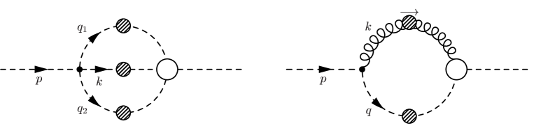
Figure C.1: Momentum routing for the sunset and for the dressing diagram in the ghost equation.

With the bare four-ghost vertex given in eq. (A.28) and the abbreviations for the squared momenta $x=p^{2}$, $y_{1}=(q_{1})^{2}$, $y_{2}=(q_{2})^{2}$, $z_{1}=(p-q_{1})^{2}$ and $z_{2}=(p-q_{1}-q_{2})^{2}$ the sunset diagram reads

$$U^{sun}=\frac{N_{c}^{2}\,g^{4}\,\tilde{Z}_{4}}{2\,(2\pi)^{8}}\left(\frac{\alpha}{2}\left(1-\frac{\alpha}{2}\right)\lambda\right)^{2}\int d^{4}q_{1}\,\frac{B\,(y_{1})^{\beta}}{x\,y_{1}}\,\int d^{4}q_{2}\,\frac{B^{2}\,(y_{2})^{\beta}\,(z_{2})^{\beta}}{y_{2}\,z_{2}}.$$ (C.23)

The factor $1/x$ in the first integral stems from the left hand side of the ghost equation. We now integrate the inner loop with the help of formula (C.9) and obtain

$$U^{sun}=\frac{N_{c}^{2}\,g^{4}\,\tilde{Z}_{4}\,B^{3}}{512\,\pi^{6}}\left(\frac{\alpha}{2}\left(1-\frac{\alpha}{2}\right)\lambda\right)^{2}\frac{\Gamma^{2}(1+\beta)\,\Gamma(-2\beta)}{\Gamma^{2}(1-\beta)\,\Gamma(2+2\beta)}\,\int d^{4}q_{1}\,\frac{(y_{1})^{\beta}}{x\,y_{1}}\,(z_{1})^{2\beta}\,,$$ (C.24)

where $z_{1}$ is the total squared momentum flowing through the integrated loop. The second integration is done in the same way. We arrive at

$$U^{sun} = x^{3\beta}\,\frac{N_{c}^{2}\,g^{4}\,\tilde{Z}_{4}\,B^{3}}{512\,\pi^{4}}\left(\frac{\alpha}{2}\left(1-\frac{\alpha}{2}\right)\lambda\right)^{2}\frac{\Gamma^{3}(1+\beta)\,\Gamma(-3\beta-1)}{\Gamma^{3}(1-\beta)\,\Gamma(3+3\beta)}$$ (C.25)

$$:= x^{3\beta}(U^{\prime})^{sun}\,.$$

As each integration step eats up the two squared momenta in the denominators of the integral kernels only powers of $x$ to the anomalous dimensions of the dressing functions in the loop (here $3\beta$ from three ghost propagators) survive. This mechanism works in the same way for all diagrams and explains the pattern in the eqs. (4.4), (4.5) and (4.6) of section 4.2.

Next we evaluate the two contributions in the gluon equation needed for the argument below eq. (4.9). The explicit expressions for the kernels of two-loop gluon diagrams are rather lengthy but the calculation is done along the same lines as in the ghost sunset diagram above. Therefore we just give the final results:

$$V^{squint}_{TTTT} = x^{4\sigma}\,\frac{-27\,g^{4}\,N_{c}^{2}\,Z_{4}\,A^{4}}{4096\,\pi^{4}}\,\frac{\Gamma(-1-4\sigma)\>\Gamma(1/2-\sigma)\>\Gamma(3\sigma)\>\Gamma^{2}(1+\sigma)}{\Gamma(4-3\sigma)\>\Gamma^{2}(2-\sigma)\>\Gamma(3/2-\sigma)\>\Gamma(4+4\sigma)}\times$$ (C.26)

$$2^{-4\sigma}\>(-1+3\sigma)\>(10+\sigma-66\sigma^{2}+63\sigma^{3})\>(5+43\sigma+47\sigma^{2})$$

$$:= x^{4\sigma}\,(V^{\prime})^{squint}_{TTTT}\,,$$

$$W^{sun}_{LLL} = x^{3\delta}\,\frac{g^{4}\,N_{c}^{2}\,Z_{4}\,C^{3}}{1536\,\pi^{4}}\,\frac{1}{(1+3\delta)}\frac{\Gamma^{3}(1+\delta)\>\Gamma(1-3\delta)}{\Gamma^{3}(2-\delta)\>\Gamma(3+3\delta)}\>\>\lambda^{3}$$ (C.27)

$$:= x^{3\delta}\,(W^{\prime})^{sun}_{LLL}\,.$$

Finally we calculate that part in the dressing diagram of the ghost equation which contains the longitudinal part of the gluon propagator for the special case $\alpha=0,2$, where $L(x)=1$. These are the linear covariant gauges. With the momentum assignments $x=p^{2}$, $y=q^{2}$ and $z=k^{2}=(p-q)^{2}$ the longitudinal part of the diagram is given by

$$U^{dress}_{L} = -\frac{N_{c}\,g^{2}\,\tilde{Z}_{1}}{(2\pi)^{4}}\int d^{4}q\,q_{\mu}\,\lambda\frac{k_{\mu}k_{\nu}}{z^{2}}p_{\nu}\frac{By^{\beta}}{x\,y}$$ (C.28)

where again the factor $1/x$ stems from the left hand side of the equation. Writing the kernel in terms of squared momenta we obtain

$$U^{dress}_{L} = -\frac{N_{c}g^{2}\,\tilde{Z}_{1}}{(2\pi)^{4}}\int d^{4}q\>\lambda\>B\>y^{\beta}\>\left(\frac{1}{2z^{2}}-\frac{x}{4yz^{2}}-\frac{y}{4xz^{2}}+\frac{1}{4xy}\right).$$ (C.29)

After integration we obtain

$$U^{dress}_{L} = -\frac{N_{c}\,g^{2}\,\tilde{Z}_{1}}{16\,\pi^{2}}\>\lambda\>B\,x^{\beta}\>\left(\frac{1}{2}-\frac{1}{4}-\frac{1}{4}+0\right)\Gamma(0)$$ (C.30)

$$= 0.$$ (C.31)

Although $\Gamma(0)$ is formally divergent this contribution vanishes due to vanishing coefficients.

C.4 Numerical methods for flat Euclidean space-time

Here we detail the numerical method we employed to solve the coupled system of ghost and gluon Dyson-Schwinger equations, (3.24) and (3.25). For the convenience of the reader we display the equations again:

$$\frac{1}{G(x)} = \tilde{Z}_{3}-g^{2}N_{c}\int\frac{d^{4}q}{(2\pi)^{4}}\frac{K(x,y,z)}{xy}G(y)Z(z)\;,$$ (C.32)

$$\frac{1}{Z(x)} = {Z}_{3}+g^{2}\frac{N_{c}}{3}\int\frac{d^{4}q}{(2\pi)^{4}}\frac{M(x,y,z)}{xy}G(y)G(z)$$ (C.33)

$$+g^{2}\frac{N_{c}}{3}\int\frac{d^{4}q}{(2\pi)^{4}}\frac{Q(x,y,z)}{xy}\frac{G(y)^{(1-a/\delta-2a)}}{Z(y)^{a}}\frac{G(z)^{(1-b/\delta-2b)}}{Z(z)^{b}}\;.$$

Recall $x=p^{2}$, $y=q^{2}$ and $z=(q-p)^{2}=x+y-2\sqrt{(}xy)\cos\Theta$. The integral over the loop momentum $q$ is transformed to four-dimensional hyperspherical coordinates. Two of the four integrals are then trivial and yield a factor of $4\pi$. The remaining angular integral and the radial integral have to be performed with the help of numerical routines. We use the Gauss-Legendre quadrature rule described in [171]. To achieve high accuracy we split the radial loop integral into three parts, $y\in[0,\epsilon^{2}]$, $y\in(\epsilon^{2},x]$ and $y\in(x,x_{UV}]$. The second split is necessary as the integrands are not smooth at the boundary $x$ and too much accuracy would be lost, if one uses a quadrature rule that spans the whole region $(\epsilon^{2},x_{UV}]$.

According to the value of their argument the dressing functions $Z$ as well as $G$ have to be handled differently. In the infrared region, $y,z\in[0,\epsilon^{2}]$, $Z$ and $G$ behave like powers and are replaced according to eq. (3.44). Recall that the approximation by leading powers in the infrared is justified by the analysis of subleading contributions at the end of subsection 3.3.2. The infrared matching point $\epsilon^{2}$ is chosen sufficiently low. In physical units we have $\epsilon^{2}=(0.55\,\mbox{MeV})^{2}$ in our calculations. In the high momentum regime, $y\in(x,x_{UV}]$, arguments $z$ occur which are larger than the numerical cutoff $x_{UV}$. There we approximate the respective dressing functions by the expressions

$$Z(z) = Z(l)\left[\omega\log\left(\frac{z}{l}\right)+1\right]^{\gamma}\;,$$ (C.34)

$$G(z) = G(l)\left[\omega\log\left(\frac{z}{l}\right)+1\right]^{\delta}\;.$$ (C.35)

according to the one loop behaviour of the solutions as has been detailed in subsection 3.3.1. Here $\omega=11N_{c}\alpha(l)/12\pi$ and the squared momentum $l$ is a perturbative scale. We chose $l=(174\,\mbox{GeV})^{2}$ to be slightly lower than the numerical cutoff $x_{UV}=(177\,\mbox{GeV})^{2}$. To be able to perform the angular integrations for momenta $[\epsilon^{2},x_{UV}]$ we expand the dressing functions in Chebychev polynomials and solve the coupled system of equations for the expansion coefficients using a Newton iteration method. Details of this technique can be found in appendix B of ref. [67].

C.5 One-loop scaling

In the framework of the truncation scheme presented in section 3.3 we have shown that the substitution

$$Z_{1}\rightarrow{\mathcal{Z}}_{1}(x,y,z;s,L)=\frac{G(y)^{(1-a/\delta-2a)}}{Z(y)^{(1+a)}}\frac{G(z)^{(1-b/\delta-2b)}}{Z(z)^{(1+b)}}$$ (C.36)

for the gluon vertex renormalisation constant $Z_{1}$ together with a bare three-gluon vertex yields the correct one-loop scaling of the gluon loop in the gluon Dyson-Schwinger equation. This is true for any values $a$ and $b$. Of course, in a full treatment of the coupled ghost-gluon system ${\mathcal{Z}}_{1}(s,L)$ would be independent of momentum. Therefore a choice of $a$ and $b$ which keeps ${\mathcal{Z}}_{1}$ as weakly varying as possible seems the most reasonable one.

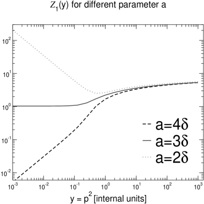
Figure C.2: The $y$-dependence of the function ${\mathcal{Z}}_{1}(y,z)$ for different values of the parameter $a$. Only the choice $a=3\delta$ leads to momentum independence in the infrared. Due to the symmetry of the ansatz for ${\cal Z}_{1}(y,z)$ the $z$-dependence is the same for $b=a$.

This choice can be inferred using the scaling of the dressing functions extracted from the renormalisation group equation, see ref. [66] for details. The dressing functions can be expressed as

$$Z(x) = \left(\frac{\alpha(x)}{\alpha(s)}\right)^{1+2\delta}R^{2}(x)\;,$$

$$G(x) = \left(\frac{\alpha(x)}{\alpha(s)}\right)^{-\delta}R^{-1}(x)\;,$$ (C.37)

where the running coupling provides the correct one loop scaling in the ultraviolet. Consequently the function $R(x)$ approaches unity for high momenta. Furthermore, from the known infrared behaviour of $Z(x)$, $G(x)$ and $\alpha(x)$ (c.f. subsection 3.3.2) one infers that $R(x)$ is proportional to $x^{\kappa}$ in the infrared. Writing ${\mathcal{Z}}_{1}$ in terms of $\alpha(x)$ and $R(x)$ yields

$${\mathcal{Z}}_{1}(x,y,z;s,L)=\left(\frac{\alpha(\mu^{2})}{\alpha(y)}\right)^{1+3\delta}R^{-3+a/\delta}(y)\left(\frac{\alpha(\mu^{2})}{\alpha(z)}\right)^{1+3\delta}R^{-3+b/\delta}(z).$$ (C.38)

In the perturbative region $R(y),R(z)\rightarrow 1$ and the function ${\mathcal{Z}}_{1}$ is therefore slowly varying for any $a$ and $b$ according to the logarithmic behaviour of the running coupling $\alpha$. In the infrared, however, $\alpha$ approaches its fixed point while the functions $R$ behaves like a power. Consequently the choice $a=b=3\delta$ guarantees the weakest momentum dependence of ${\mathcal{Z}}_{1}$ which is illustrated in Fig. C.2. Shown is the $y$-dependence of the function ${\mathcal{Z}}_{1}(x,y,z=y;s,L)$. (Note also that due to the symmetry ${\mathcal{Z}}_{1}(x,y,z;s,L)={\mathcal{Z}}_{1}(x,z,y;s,L)$ and the absence of an explicit $x$-dependence this is sufficient to demonstrate its momentum dependence.) In the perturbative momentum regime the function ${\mathcal{Z}}_{1}$ does not vary with the parameter $a$. So all three choices give the same logarithmic running in momentum as required to give the correct one loop scaling behaviour of the integral. In the infrared, however, a change in $a$ gives rise to substantial changes in the behaviour of ${\mathcal{Z}}_{1}$, with only the choice $a=3\delta$ leading to a constant.

Appendix D Discretisation and finite volume effects

D.1 Radial discretised DSEs

In this appendix we study possible discretisation errors in the Dyson-Schwinger equations. We investigate a discretised version of the angular approximated DSEs in the ghost-loop only truncation scheme discussed in subsection 5.1.2. From the infrared analysis of these DSEs one finds power laws for the ghost and gluon dressing functions. These power laws are used in the numerical treatment of eqs. (5.13), (5.14) to solve the integrals from zero momentum to an infrared matching point $\epsilon^{2}$. It has been claimed that these integrals are crucial to find numerical solutions for the ghost and gluon propagators [67]. In this section we will show that they are not. We will introduce a prescription to discretise the radial integrals in the DSEs such that the smallest momentum showing up in the equations is nonzero. Despite the infrared divergence of the ghost dressing function we reproduce the solutions from the formulation with continuous momenta without having to include the region in the very infrared. This is very important as otherwise the attempt to solve Dyson-Schwinger equations on a four-torus, performed in chapter 5, might be hopeless from the very beginning.

For the discretisation of eqs. (5.13), (5.14) we use the same prescription for the radial integral as one gets for all four Cartesian momentum directions if employing a finite volume. Note that contrary to the finite volume case there is no easy geometrical interpretation for a discretised radial integral.

With $l$ denoting the inverse spacing of the radial momentum $q$, we thus substitute

$$\int dq^{2}=\int dq\>2q\>\longrightarrow\>\left(\frac{2\pi}{l}\right)\sum_{j}2\left(\frac{2\pi}{l}j\right)=\left(\frac{2\pi}{l}\right)^{2}\sum_{j}2j\,,$$ (D.1)

into eqs. (5.13), (5.14). We obtain

$$\frac{1}{G(x_{i})} = \tilde{Z}_{3}-\frac{9}{4}\frac{g^{2}N_{c}}{48\pi^{2}}\left(\frac{2\pi}{l}\right)^{2}\left[Z(x_{i})\sum_{j=1}^{i-1}\frac{2j}{x_{i}}\frac{y_{j}}{x_{i}}G(y_{j})+\sum_{j=i}^{N}\frac{2j}{y_{j}}Z(y_{j})G(y_{j})\right]\,,$$ (D.2)

$$\frac{1}{Z(x_{i})} = Z_{3}+\frac{g^{2}N_{c}}{48\pi^{2}}\left(\frac{2\pi}{l}\right)^{2}\left[G(x_{i})\sum_{j=1}^{i-1}\frac{2j}{x_{i}}\left(-\frac{y_{j}^{2}}{x_{i}^{2}}+\frac{3y_{j}}{2x_{i}}\right)G(y_{j})+\sum_{j=i}^{N}\frac{2j}{2y_{j}}G^{2}(y_{j})\right]\,.$$

The squared momenta $x_{i}$ are given as $x_{i}=\left(i\,2\pi/l\right)^{2}$. The largest momentum $x_{N}$ corresponds to the numerical cutoff $L=\Lambda^{2}$ in the continuous version, eqs. (5.13), (5.14). The momentum $x_{0}=0$ is discarded in the calculation. We solve the discretised eqs. (D.2), (LABEL:gluon-rad) by iteration employing the Newton method. To directly compare the continuous solution with the discretised one we use the same cut-off and renormalise at the same momentum. This is most easily done by taking $Z_{3}(\mu^{2},\Lambda^{2})$ and $\tilde{Z}_{3}(\mu^{2},\Lambda^{2})$ in eqs. (D.2), (LABEL:gluon-rad) from the continuum solution.

It is quite amusing that there is a second way to solve eqs. (D.2), (LABEL:gluon-rad), which corresponds to the conversion of the continuous integral equations (5.13) and (5.14) into differential equations, see ref. [67]: Subtract eqs. (D.2), (LABEL:gluon-rad) from themselves for two different arbitrary momenta $x_{i}$ and $x_{s}$. One obtains

$$\frac{1}{G(x_{i})} = \frac{1}{G(x_{s})}-\frac{9}{4}\frac{g^{2}N_{c}}{48\pi^{2}}\left(\frac{2\pi}{l}\right)^{2}\left[Z(x_{i})\sum_{j=1}^{i-1}\frac{2j}{x_{i}}\frac{y_{j}}{x_{i}}G(y_{j})-Z(x_{s})\sum_{j=1}^{s-1}\frac{2j}{x_{s}}\frac{y_{j}}{x_{s}}G(y_{j})\right.$$ (D.4)

$$\hskip 170.71652pt+\left.\sum_{j=min(i,s)}^{min(i-1,s-1)}\frac{2j}{y_{j}}Z(y_{j})G(y_{j})\right]\,,$$

$$\frac{1}{Z(x_{i})} = \frac{1}{Z(x_{s})}+\frac{g^{2}N_{c}}{48\pi^{2}}\left(\frac{2\pi}{l}\right)^{2}\left[G(x_{i})\sum_{j=1}^{i-1}\frac{2j}{x_{i}}\left(-\frac{y_{j}^{2}}{x_{i}^{2}}+\frac{3y_{j}}{2x_{i}}\right)G(y_{j})\right.$$ (D.5)

$$\hskip 28.45274pt\left.-G(x_{s})\sum_{j=1}^{s-1}\frac{2j}{x_{s}}\left(-\frac{y_{j}^{2}}{x_{s}^{2}}+\frac{3y_{j}}{2x_{s}}\right)G(y_{j})+\sum_{j=min(i,s)}^{min(i-1,s-1)}\frac{2j}{2y_{j}}G^{2}(y_{j})\right]\,.$$

         

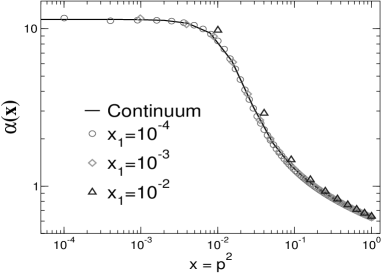
Figure D.1: Comparison of the gluon dressing function $Z(x)$, the ghost dressing function $G(x)$ and the running coupling $\alpha(x)$ obtained from the DSEs with continuous momenta and from the discretised version. For the radial grid of the discretised version we used three different momentum spacings.

If we now set $s=1$ the sums in the equations run from $j=1..i$. Given the values for $Z(x_{1})$ and $G(x_{1})$ the equations for $Z(x_{2})$ and $G(x_{2})$ are then simple quadratic equations which can be solved easily. Given these solutions we can solve the equations for $i=3$ and so on. The complete solution is thereby built point for point from the infrared to the ultraviolet region of momentum. The advantage of this method is that one does not have to use a numerical iteration procedure to solve the equations. Of course, the specification of the input values $Z(x_{1})$ and $G(x_{1})$ corresponds to a certain choice of the renormalisation constants $Z_{3}(\mu^{2},\Lambda^{2})$ and $\tilde{Z}_{3}(\mu^{2},\Lambda^{2})$, i.e. to the boundary restriction from a certain choice of renormalisation point. The disadvantage of this method is thus that one has to improve iteratively on the input values $Z(x_{1})$ and $G(x_{1})$ until the same $Z_{3}(\mu^{2},\Lambda^{2})$ and $\tilde{Z}_{3}(\mu^{2},\Lambda^{2})$ are obtained as for the continuous integral equations. Both ways of solving eqs. (D.2), (LABEL:gluon-rad) certainly yield the same results.

Our solutions for the dressing functions on the radial momentum grid are compared with the solutions from the continuum in Fig. D.1. For the dressing functions and the running coupling we find nearly the same results with both methods. There are only small discretisation errors for our largest momentum spacing. For smaller spacings these errors become more and more irrelevant and we thus conclude that there is a smooth transition to the continuum as the spacing more and more decreases.

D.2 The influence of zero modes on the solutions of DSEs on a torus

An important point when formulating the Dyson–Schwinger equations on the torus could be the treatment of the zero modes. In addition, on the torus an infrared analysis like the one in flat Euclidean space-time is not possible, and one is left with the problem how the dressing functions behave at vanishing momenta. Guided by the intuition that especially the long ranged modes should be affected by the finite volume we assume in the following $Z(x\rightarrow 0)=0$ just like in the continuum and $G(x\rightarrow 0)=const$ if zero modes are neglected. Phrased otherwise we assume that the zero modes are the missing ingredient to ensure the correct infinite volume limit for the torus results. Therefore, if on tori of different volumes $G(x=0)$ shows no sign of becoming divergent, the infrared enhancement seen in $G(x\rightarrow 0)$ or in the flat space-time results has to be due to the torus zero modes of gluons and ghosts.

Therefore, in this appendix, we will show that the assumption $G(x=0)<\infty$ does not lead to a contradiction in the equations on the torus if zero modes are neglected. To this end we focus on the truncation scheme without angular approximations. First we rewrite eqs. (3.24), (3.25) as

$$\frac{1}{G(x)} = Z_{3}-g^{2}N_{c}\int\frac{d^{4}q}{(2\pi)^{4}}\frac{K(x,y,z)}{xy}G(y)Z(z)\;,$$ (D.6)

$$\frac{1}{Z(x)} = \tilde{Z}_{3}+g^{2}\frac{N_{c}}{3}\int\frac{d^{4}q}{(2\pi)^{4}}\frac{M(x,y,z)}{xy}G(y)G(z)$$ (D.7)

$$\hskip 17.07182pt+\,g^{2}\frac{N_{c}}{3}\int\frac{d^{4}q}{(2\pi)^{4}}\frac{Q(x,y,z)}{xy}\frac{G(y)^{-2-6\delta}}{Z(y)^{3\delta}}\frac{G(z)^{-2-6\delta}}{Z(z)^{3\delta}}\;.$$

According to Appendix C.5 we have chosen $a=b=3\delta$, where $\delta=-9/44$, the anomalous dimension of the ghost. The kernels have the form:

$$K(x,y,z) = \frac{1}{z^{2}}\left(-\frac{(x-y)^{2}}{4}\right)+\frac{1}{z}\left(\frac{x+y}{2}\right)-\frac{1}{4}=xy\frac{\sin^{2}\Theta}{z^{2}}\;,$$ (D.8)

$$M(x,y,z) = \frac{1}{z}\left(\frac{\zeta-2}{4}x+\frac{y}{2}-\frac{\zeta}{4}\frac{y^{2}}{x}\right)+\frac{1}{2}+\frac{\zeta}{2}\frac{y}{x}-\frac{\zeta}{4}\frac{z}{x}\;,$$ (D.9)

$$Q^{\prime}(x,y,z) = \frac{1}{z^{2}}\left(\frac{1}{8}\frac{x^{3}}{y}+x^{2}-\frac{19-\zeta}{8}xy+\frac{5-\zeta}{4}y^{2}+\frac{\zeta}{8}\frac{y^{3}}{x}\right)$$ (D.10)

$$+\frac{1}{z}\left(\frac{x^{2}}{y}-\frac{15+\zeta}{4}x-\frac{17-\zeta}{4}y+\zeta\frac{y^{2}}{x}\right)$$

$$-\left(\frac{19-\zeta}{8}\frac{x}{y}-\frac{3-4\zeta}{2}+\frac{9\zeta}{4}\frac{y}{x}\right)$$

$$+z\left(\frac{\zeta}{x}+\frac{5-\zeta}{4y}\right)+z^{2}\frac{\zeta}{8xy}\;.$$

We first analyse the behaviour of the integrands in the limit $y\rightarrow 0$ for finite momenta $x$. Then $Z(z)\rightarrow Z(x)$ and $G(z)\rightarrow G(x)$ and the kernels times the respective dressing functions are to appropriate order in momentum $y$:

$$\frac{G(y)Z(z)}{xy}K(x,y,z) \rightarrow G(0)Z(x)\frac{\sin^{2}\Theta}{x^{2}}\;,$$ (D.11)

$$\frac{G(y)G(z)}{xy}M(x,y,z) \rightarrow G(0)G(x)\frac{1}{x^{2}}\left(1+(\zeta-2)\cos^{2}\Theta\right)\;,$$ (D.12)

$$\frac{G(y)^{-2-6\delta}G(y)^{-2-6\delta}}{Z(y)^{3\delta}Z(z)^{3\delta}xy}Q^{\prime}(x,y,z) \rightarrow \frac{G(0)^{-2-6\delta}G(x)^{-2-6\delta}}{Z(0)^{3\delta}Z(x)^{3\delta}xy}\left(\frac{\zeta\cos^{2}\Theta}{xy}+...\right)\;.$$ (D.13)

Furthermore, $z=x+y-2\sqrt{xy}\cos\Theta$ has been used and terms proportional to $\cos\Theta$ have been dropped, as they either integrate to zero in the continuum or cancel each other in the sums on the torus. Each of the expressions (D.11), (D.12), (D.13) is then the appropriate term for $j=0$ on the right hand side of the Dyson-Schwinger equations on the torus. Clearly one observes that only a finite ghost mode $G(0)$ avoids trouble with divergences. This is especially true for the kernel $Q^{\prime}$ of the gluon loop, as $Z^{-3\delta}(y\rightarrow 0)$ is more singular than the simple pole, so this kernel vanishes for small momenta $y$. The other two expressions (D.11) and (D.12) are finite. One is then left with the ambiguous quantities $\sin^{2}\Theta$ and $\cos^{2}\Theta$ which will be replaced by their integrals from zero to $2\pi$ in the calculation at the end of this section. The arbitrariness of this procedure is considerably moderated by the observation that any number plugged in for the trigonometric functions yields the same qualitative result at the end of this section.

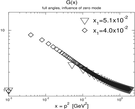
Figure D.2: $G(0)$ compared with the results for finite momentum $x$ on the torus. For convenience we have kept the logarithmic momentum scale and plotted the zero modes on the left border of the figure.

Second, we take the limit $z\rightarrow 0$, which on the torus is identical to $\Theta\rightarrow 0$. The ghost kernel $\sin^{2}\Theta/z^{2}$ alone would certainly diverge as $\Theta\rightarrow 0$, but taking into account the power law behaviour $Z(z)\sim z^{2\kappa}$ for the gluon dressing function the integrand is zero in this limit. This is valid for $\kappa>0.5$, which is in agreement with the infrared analysis in the continuum. We therefore may omit the points $z=0$ in the ghost equation. The situation is different in the gluon equation where the kernel of the ghost loop has a finite limit $z\rightarrow 0$: $M(x,x,0)/xy=(\zeta+1)/(2x^{2})$. Therefore with a finite ghost dressing function $G(0)$ the points $z=0$ in the ghost loop contribute but no divergences occur. In the gluon loop the kernel $Q^{\prime}$ multiplied by the dressing functions approaches zero for vanishing momentum $z$ due to the power law behaviour of $Z^{-3\delta}(z\rightarrow 0)$.

To obtain a definite value for $G(0)$ we now investigate the behaviour of the eqs. (D.6), (D.7) in the limit $x\rightarrow 0$. The integrands are then given by

$$\frac{G(y)Z(z)}{xy}K(x,y,z) \rightarrow G(y)Z(y)\frac{\sin^{2}\Theta}{y^{2}}\;,$$ (D.14)

$$\frac{G(y)G(z)}{xy}M(x,y,z) \rightarrow G(y)G(y)\left(\frac{1-\zeta\cos^{2}\Theta}{xy}+...\right)\;,$$ (D.15)

where the kernel $Q^{\prime}$ is of no interest, as we know the gluon loop to be subleading in the infrared. Clearly, the kernel $M$ of the ghost loop in the gluon equation is now singular for $x\rightarrow 0$, corresponding to a vanishing gluon dressing function in the infrared. This result confirms our working hypothesis that the gluon mode $Z(0)$ is not affected by the finite volume of the torus. The integrand of the ghost equation is finite up to the point $y=0$. There the pole in the kernel is cancelled by the behaviour of the gluon dressing function $Z(y)\sim y^{2\kappa}$ resulting in a zero for vanishing momentum $x$ and $y$.

We therefore arrive at a consistent set of equations for the ghost propagator at $p^{2}=0$ and a vanishing gluon $Z(0)$. In Fig. D.2 we show the results for the ghost dressing function gained on two different volumes on the torus. Within numerical accuracy the values of $G(0)$ are the same for the two volumes. Obviously terms with high loop momentum $y$ contribute most to the right hand side of the ghost equation for vanishing momentum $x$. Furthermore, one observes that the actual value of $G(0)$ is not in accordance with an extrapolation of the ghost curves to the infrared. There is also no sizeable change of the gluon and the ghost dressing function when $G(0)$ is set to zero by hand. This has been done in all calculations performed in chapter 5.

Having shown that $G(0)<\infty$ on the torus even in the infinite-volume limit and assuming that the torus should provide a reasonable infrared regularisation of physics in flat space-time we conclude that the divergence of $G(0)$ is very probably due to the torus zero modes of gluons and ghosts. Noting furthermore that a diverging $G(0)$ is related to Zwanziger’s horizon condition and the Kugo–Ojima confinement criterion this indicates a direct relation between zero modes, the Gribov horizon and confinement.

Bibliography

- [1] C. Itzykson and J. B. Zuber, “Quantum Field Theory,”. New York, Usa: Mcgraw-hill (1980) 705 P.(International Series In Pure and Applied Physics).
- [2] R. J. Rivers, “Path Integral Methods In Quantum Field Theory,”. Cambridge, UK: Univ. Pr. (1987) 339 p. (Cambridge monographs on mathematical physics).
- [3] T. P. Cheng and L. F. Li, “Gauge theory of elementary particle physicsS,”. Oxford, Uk: Clarendon ( 1984) 536 P. ( Oxford Science Publications).
- [4] S. Weinberg, “The Quantum theory of fields. Vol. 1-3,”. Cambridge, UK: Univ. Pr. (1996).
- [5] M. E. Peskin and D. V. Schroeder, “An Introduction to quantum field theory,”. Reading, USA: Addison-Wesley (1995) 842 p.
- [6] T. Muta, Foundations of quantum chromodynamics. World Scientific, 1998. Singapore.
- [7] W. J. Marciano and H. Pagels, “Quantum Chromodynamics: a review,” Phys. Rept. 36 (1978) 137.
- [8] F. Karsch, “Lattice results on QCD thermodynamics,” Nucl. Phys. A698 (2002) 199–208, hep-ph/0103314.
- [9] C. D. Roberts and S. M. Schmidt, “Dyson-Schwinger equations: Density, temperature and continuum strong QCD,” Prog. Part. Nucl. Phys. 45 (2000) S1–S103, nucl-th/0005064.
- [10] R. Alkofer and L. von Smekal, “The infrared behavior of QCD Green’s functions: Confinement, dynamical symmetry breaking, and hadrons as relativistic bound states,” Phys. Rept. 353 (2001) 281, hep-ph/0007355.
- [11] M. Creutz, “Lattice gauge theory: A retrospective,” Nucl. Phys. Proc. Suppl. 94 (2001) 219–226, hep-lat/0010047.
- [12] L. Baulieu and J. Thierry-Mieg, “The principle of BRS symmetry: an alternative approach to Yang-Mills theories,” Nucl. Phys. B197 (1982) 477.
- [13] S. Pokorski, “Gauge field theories,”. Cambridge, Uk: Univ. Pr. ( 1987) 394 P. ( Cambridge Monographs On Mathematical Physics).
- [14] L. D. Faddeev and V. N. Popov, “Feynman diagrams for the Yang-Mills field,” Phys. Lett. B25 (1967) 29–30.
- [15] L. Baulieu and M. Schaden, “Gauge Group TQFT and Improved Perturbative Yang-Mills Theory,” Int. J. Mod. Phys. A13 (1998) 985–1012, hep-th/9601039.
- [16] M. Schaden, “Quantization in the presence of Gribov ambiguities,” hep-th/9810162.
- [17] G. Parisi and Y.-s. Wu, “Perturbation theory without gauge fixing,” Sci. Sin. 24 (1981) 483.
- [18] D. Zwanziger, “Time-independent stochastic quantization, DS equations, and infrared critical exponents in QCD,” hep-th/0206053.
- [19] J. Thierry-Mieg, “Ghost creating gauges in Yang-Mills theory,” Nucl. Phys. B261 (1985) 55.
- [20] N. Nakanishi and I. Ojima, Covariant Operator Formalism Of Gauge Theories And Quantum Gravity. No. 27. World Scientific lecture notes in physics, 1990.
- [21] M. Quandt and H. Reinhardt, “Ward identities for Yang-Mills theory in Abelian gauges: Abelian dominance at high energies,” Phys. Lett. B424 (1998) 115–124, hep-th/9712181.
- [22] M. Quandt and H. Reinhardt, “Field strength formulation of SU(2) Yang-Mills theory in the maximal Abelian gauge: Perturbation theory,” Int. J. Mod. Phys. A13 (1998) 4049–4076, hep-th/9707185.
- [23] M. Schaden, “SU(2) gauge theory in covariant (maximal) Abelian gauges,” hep-th/0003030.
- [24] H. Leutwyler, “Principles of chiral perturbation theory,” hep-ph/9406283.
- [25] G. Ecker, “Chiral perturbation theory,” Prog. Part. Nucl. Phys. 35 (1995) 1–80, hep-ph/9501357.
- [26] A. V. Manohar, “Effective field theories,” hep-ph/9606222.
- [27] G. Ecker, “Chiral symmetry,” hep-ph/9805500.
- [28] P. C. Tandy, “Hadron physics from the global color model of QCD,” Prog. Part. Nucl. Phys. 39 (1997) 117–199, nucl-th/9705018.
- [29] Y. Nambu and G. Jona-Lasinio, “Dynamical model of elementary particles based on an analogy with superconductivity. I,” Phys. Rev. 122 (1961) 345–358.
- [30] Y. Nambu and G. Jona-Lasinio, “Dynamical model of elementary particles based on an analogy with superconductivity. II,” Phys. Rev. 124 (1961) 246–254.
- [31] R. Alkofer and H. Reinhardt, “Chiral quark dynamics,”. Berlin, Germany: Springer (1995) 114 p. (Lecture notes in physcis).
- [32] W. Hollik, “The electroweak standard model,”. Published in *Trieste 1999, Particle physics* 1-52.
- [33] M. Z. Iofa and I. V. Tyutin, “Gauge invariance of spontaneously broken nonabelian theories in the Bogolyubov-Parasiuk-Hepp-Zimmermann method. (in Russian),” Teor. Mat. Fiz. 27 (1976) 38–47.
- [34] C. Becchi, A. Rouet, and R. Stora, “Renormalization of gauge theories,” Annals Phys. 98 (1976) 287–321.
- [35] S. Elitzur, “Impossibility of spontaneously breaking local symmetries,” Phys. Rev. D12 (1975) 3978–3982.
- [36] K. Fujikawa, “Dynamical stability of the BRS supersymmetry and the Gribov problem,” Nucl. Phys. B223 (1983) 218.
- [37] R. Haag, “Local quantum physics: Fields, particles, algebras,”. Berlin, Germany: Springer (1992) 356 p. (Texts and monographs in physics).
- [38] H. Lehmann, K. Symanzik, and W. Zimmermann, “On the formulation of quantized field theories,” Nuovo Cim. 1 (1955) 205–225.
- [39] T. Kugo and I. Ojima, “Local covariant operator formalism of nonabelian gauge theories and quark confinement problem,” Prog. Theor. Phys. Suppl. 66 (1979) 1.
- [40] J. Baez and J. P. Muniain, “Gauge fields, knots and gravity,”. Singapore, Singapore: World Scientific (1994) 465 p. (Series on knots and everything, 4).
- [41] F. Strocchi, “Local and covariant gauge quantum field theories. Cluster property, superselection rules, and the infrared problem,” Phys. Rev. D17 (1978) 2010–2021.
- [42] R. P. Feynman, “The qualitative behavior of Yang-Mills theory in (2+1)- dimensions,” Nucl. Phys. B188 (1981) 479.
- [43] T. Kugo, “The Universal Renormalization Factors and Color Confinement Condition in Non-Abelian Gauge Theory,” hep-th/9511033.
- [44] H. Nakajima, S. Furui, and A. Yamaguchi, “Numerical study of the Kugo-Ojima criterion and the Gribov problem in the Landau gauge,” hep-lat/0007001.
- [45] H. Nakajima and S. Furui, “Numerical tests of the Kugo-Ojima color confinement criterion,” hep-lat/0006002.
- [46] H. Nakajima and S. Furui, “Numerical studies of confinement in the Landau gauge by the larger lattice simulation,” hep-lat/0208074.
- [47] H. Suman and K. Schilling, “First Lattice Study of Ghost Propagators in SU(2) and SU(3) Gauge Theories,” Phys. Lett. B373 (1996) 314–318, hep-lat/9512003.
- [48] K. Langfeld et al., “Vortex induced confinement and the IR properties of Green functions,” hep-th/0209173.
- [49] J. C. R. Bloch, A. Cucchieri, K. Langfeld, and T. Mendes, “Running coupling constant and propagators in SU(2) Landau gauge,” hep-lat/0209040.
- [50] A. Wightman, “Quelque problèmes mathématique de la thèorie quantique relativiste,”. In: Lecture notes, Faculté des Sciences, Univ. de Paris 1957.
- [51] K. Osterwalder and R. Schrader, “Axioms for Euclidean Green’s functions,” Commun. Math. Phys. 31 (1973) 83–112.
- [52] K. Osterwalder and R. Schrader, “Axioms for Euclidean Green’s functions. 2,” Commun. Math. Phys. 42 (1975) 281.
- [53] V. Sauli and J. Adam, “Solving the Schwinger-Dyson equation for a scalar propagator in Minkowski space,” hep-ph/0110298.
- [54] V. Sauli, “Minkowski solution of Dyson-Schwinger equations in momentum subtraction scheme,” hep-ph/0209046.
- [55] D. Zwanziger, “Critical limit of lattice gauge theory,” Nucl. Phys. B378 (1992) 525–590.
- [56] D. Zwanziger, “Renormalizability of the critical limit of lattice gauge theory by BRS invariance,” Nucl. Phys. B399 (1993) 477–513.
- [57] V. N. Gribov, “Quantization of non-Abelian gauge theories,” Nucl. Phys. B139 (1978) 1.
- [58] P. van Baal, “Gribov ambiguities and the fundamental domain,” hep-th/9711070.
- [59] D. Zwanziger, “Nonperturbative modification of the Faddeev-Popov formula and banishment of the naive vacuum,” Nucl. Phys. B209 (1982) 336.
- [60] P. van Baal, “More (thoughts on) Gribov copies,” Nucl. Phys. B369 (1992) 259–275.
- [61] D. Zwanziger, “Fundamental modular region, Boltzmann factor and area law in lattice gauge theory,” Nucl. Phys. B412 (1994) 657–730.
- [62] D. Zwanziger, “Non-perturbative Landau gauge and infrared critical exponents in QCD,” Phys. Rev. D65 (2002) 094039, hep-th/0109224.
- [63] D. Zwanziger, “Vanishing of zero momentum lattice gluon propagator and color confinement,” Nucl. Phys. B364 (1991) 127–161.
- [64] E. Eichten and F. Feinberg, “Dynamical symmetry breaking of nonabelian gauge symmetries,” Phys. Rev. D10 (1974) 3254–3279.
- [65] K. Langfeld, H. Reinhardt, and J. Gattnar, “Gluon propagators and quark confinement,” Nucl. Phys. B621 (2002) 131–156, hep-ph/0107141.
- [66] L. von Smekal, R. Alkofer, and A. Hauck, “The infrared behavior of gluon and ghost propagators in Landau gauge QCD,” Phys. Rev. Lett. 79 (1997) 3591–3594, hep-ph/9705242.
- [67] D. Atkinson and J. C. R. Bloch, “Running coupling in non-perturbative QCD. I: Bare vertices and y-max approximation,” Phys. Rev. D58 (1998) 094036, hep-ph/9712459.
- [68] P. Watson and R. Alkofer, “Verifying the Kugo-Ojima confinement criterion in Landau gauge QCD,” Phys. Rev. Lett. 86 (2001) 5239, hep-ph/0102332.
- [69] R. Alkofer, L. von Smekal, and P. Watson, “The Kugo-Ojima confinement criterion from Dyson-Schwinger equations,” hep-ph/0105142.
- [70] C. Lerche and L. von Smekal, “On the infrared exponent for gluon and ghost propagation in Landau gauge QCD,” Phys. Rev. D65 (2002) 125006, hep-ph/0202194.
- [71] J. E. Mandula, “The gluon propagator,” Phys. Rept. 315 (1999) 273–284.
- [72] F. D. R. Bonnet, P. O. Bowman, D. B. Leinweber, and A. G. Williams, “Infrared behavior of the gluon propagator on a large volume lattice,” Phys. Rev. D62 (2000) 051501, hep-lat/0002020.
- [73] F. D. R. Bonnet, P. O. Bowman, D. B. Leinweber, A. G. Williams, and J. M. Zanotti, “Infinite volume and continuum limits of the Landau-gauge gluon propagator,” Phys. Rev. D64 (2001) 034501, hep-lat/0101013.
- [74] A. Cucchieri, “The lattice gluon propagator into the next millennium,” hep-lat/9908050.
- [75] A. Cucchieri and D. Zwanziger, “Fit to gluon propagator and Gribov formula,” Phys. Lett. B524 (2002) 123–128, hep-lat/0012024.
- [76] A. Cucchieri, “Infrared behavior of the gluon propagator in lattice Landau gauge,” Phys. Lett. B422 (1998) 233–237, hep-lat/9709015.
- [77] A. Cucchieri, “Gribov copies in the minimal Landau gauge: The influence on gluon and ghost propagators,” Nucl. Phys. B508 (1997) 353–370, hep-lat/9705005.
- [78] C. Alexandrou, P. de Forcrand, and E. Follana, “The gluon propagator without lattice Gribov copies,” Phys. Rev. D63 (2001) 094504, hep-lat/0008012.
- [79] L. von Smekal, A. Hauck, and R. Alkofer, “A solution to coupled Dyson-Schwinger equations for gluons and ghosts in Landau gauge,” Ann. Phys. 267 (1998) 1, hep-ph/9707327.
- [80] A. Hauck, The Infrared Behaviour of Gluon and Ghost Propagators in Landau Gauge QCD. PhD thesis, Universität Tübingen, 1998.
- [81] J. C. Taylor, “Ward identities and charge renormalization of the Yang-Mills field,” Nucl. Phys. B33 (1971) 436–444.
- [82] D. Atkinson and J. C. R. Bloch, “QCD in the infrared with exact angular integrations,” Mod. Phys. Lett. A13 (1998) 1055–1062, hep-ph/9802239.
- [83] C. S. Fischer, R. Alkofer, and H. Reinhardt, “The elusiveness of infrared critical exponents in Landau gauge Yang-Mills theories,” Phys. Rev. D65 (2002) 094008, hep-ph/0202195.
- [84] C. S. Fischer and R. Alkofer, “Infrared exponents and running coupling of SU(N) Yang-Mills theories,” Phys. Lett. B536 (2002) 177–184, hep-ph/0202202.
- [85] J. C. R. Bloch, “Multiplicative renormalizability of gluon and ghost propagators in QCD,” Phys. Rev. D64 (2001) 116011, hep-ph/0106031.
- [86] L. von Smekal, P. A. Amundsen, and R. Alkofer, “A Covariant model for dynamical chiral symmetry breaking in QCD,” Nucl. Phys. A529 (1991) 633–652.
- [87] V. P. Gusynin, A. W. Schreiber, T. Sizer, and A. G. Williams, “Chiral symmetry breaking in dimensionally regularized nonperturbative quenched QED,” Phys. Rev. D60 (1999) 065007, hep-th/9811184.
- [88] A. W. Schreiber, T. Sizer, and A. G. Williams, “Dimensionally regularized study of nonperturbative quenched QED,” Phys. Rev. D58 (1998) 125014, hep-ph/9804385.
- [89] N. Brown and M. R. Pennington, “Studies of confinement: how quarks and gluons propagate,” Phys. Rev. D38 (1988) 2266.
- [90] N. Brown and M. R. Pennington, “Studies of confinement: how the gluon propagates,” Phys. Rev. D39 (1989) 2723.
- [91] A. Hauck, L. von Smekal, and R. Alkofer, “Solving the gluon Dyson-Schwinger equation in the Mandelstam approximation,” Comput. Phys. Commun. 112 (1998) 149, hep-ph/9604430.
- [92] P. Watson, “Perturbative constraints on the Slavnov-Taylor identity for the ghost-gluon vertex in QCD,” hep-ph/9901454.
- [93] P. Watson, The Inclusion of Ghosts in Landau Gauge Schwinger-Dyson Studies of Infrared QCD. PhD thesis, University of Durham, 2000.
- [94] C. Lerche, “Analyse des Infrarotverhaltens von Gluon- und Geistpropagator in der QCD in Landau-Eichung.” Diploma thesis (in German), Universität Erlangen-Nürnberg, 2001.
- [95] S. Mandelstam, “Approximation scheme for QCD,” Phys. Rev. D20 (1979) 3223.
- [96] J. A. M. Vermaseren, “New features of FORM,” math-ph/0010025.
- [97] H. Gies, “Running coupling in Yang-Mills theory: A flow equation study,” Phys. Rev. D66 (2002) 025006, hep-th/0202207.
- [98] K. A. Milton and I. L. Solovtsov, “Analytic perturbation theory in QCD and Schwinger’s connection between the beta function and the spectral density,” Phys. Rev. D55 (1997) 5295–5298, hep-ph/9611438.
- [99] K. A. Milton and O. P. Solovtsova, “Analytic perturbation theory: A new approach to the analytic continuation of the strong coupling constant alpha(s) into the timelike region,” Phys. Rev. D57 (1998) 5402–5409, hep-ph/9710316.
- [100] K. A. Milton, I. L. Solovtsov, O. P. Solovtsova, and V. I. Yasnov, “Renormalization scheme and higher loop stability in hadronic tau decay within analytic perturbation theory,” Eur. Phys. J. C14 (2000) 495–501, hep-ph/0003030.
- [101] D. V. Shirkov, “Analytic perturbation theory in analyzing some QCD observables,” Eur. Phys. J. C22 (2001) 331–340, hep-ph/0107282.
- [102] Particle Data Group Collaboration, K. Hagiwara et al., “Review of particle physics,” Phys. Rev. D66 (2002) 010001.
- [103] R. Alkofer, C. S. Fischer, and L. von Smekal, “The infrared behaviour of the running coupling in Landau gauge QCD,” Acta Phys. Slov. 52 (2002) 191, hep-ph/0205125.
- [104] R. Alkofer, C. S. Fischer, and L. von Smekal, “Infrared exponents and the running coupling of Landau gauge QCD and their relation to confinement,” hep-ph/0209366.
- [105] OPAL Collaboration, K. Ackerstaff et al., “Measurement of the strong coupling constant alpha(s) and the vector and axial-vector spectral functions in hadronic tau decays,” Eur. Phys. J. C7 (1999) 571–593, hep-ex/9808019.
- [106] B. V. Geshkenbein, “Hadronic tau decay, the renormalization group, analyticity of the polarization operators and QCD parameters,” hep-ph/0206094.
- [107] K. Langfeld, “Vortex induced confinement and the Kugo-Ojima confinement criterion,” hep-lat/0204025.
- [108] K. Langfeld, H. Reinhardt, and J. Gattnar, “Manifestation of confinement in the gluon propagator,” Nucl. Phys. Proc. Suppl. 106 (2002) 673–675, hep-lat/0110025.
- [109] R. Alkofer, C. Fischer, H. Reinhardt, and L. von Smekal, “On the infrared behaviour of Gluons and Ghosts in Ghost-Antighost symmetric gauges,” hep-th/0304134. Submitted to Phys. Rev. D.
- [110] N. P. Landsman and C. G. van Weert, “Real and imaginary time field theory at finite temperature and density,” Phys. Rept. 145 (1987) 141.
- [111] H. Leutwyler and A. Smilga, “Spectrum of Dirac operator and role of winding number in QCD,” Phys. Rev. D46 (1992) 5607–5632.
- [112] G. ’t Hooft, “A property of electric and magnetic flux in nonabelian gauge theories,” Nucl. Phys. B153 (1979) 141.
- [113] P. van Baal, Twisted Boundary Conditions: A Nonperturbative Probe For Pure Nonabelian Gauge Theories. PhD thesis, Utrecht, 1984. INIS-mf-9631.
- [114] A. Hauck, L. von Smekal, and R. Alkofer, “Solving a coupled set of truncated QCD Dyson-Schwinger equations,” Comput. Phys. Commun. 112 (1998) 166, hep-ph/9804376.
- [115] H. Hata and T. Kugo, “An operator formalism of statistical mechanics of gauge theory in covariant gauges,” Phys. Rev. D21 (1980) 3333.
- [116] H. Reinhardt, “Emergence of the Haar measure in the standard functional integral representation of the Yang-Mills partition function,” Mod. Phys. Lett. A11 (1996) 2451.
- [117] J. I. Skullerud and A. G. Williams, “Quark propagator in Landau gauge,” Phys. Rev. D63 (2001) 054508, hep-lat/0007028.
- [118] J. Skullerud, D. B. Leinweber, and A. G. Williams, “Nonperturbative improvement and tree-level correction of the quark propagator,” Phys. Rev. D64 (2001) 074508, hep-lat/0102013.
- [119] CSSM Lattice Collaboration, F. D. R. Bonnet, P. O. Bowman, D. B. Leinweber, A. G. Williams, and J.-b. Zhang, “Overlap quark propagator in Landau gauge,” Phys. Rev. D65 (2002) 114503, hep-lat/0202003.
- [120] F. D. R. Bonnet, D. B. Leinweber, A. G. Williams, J. M. Zanotti, and J. B. Zhang, “Quark propagator in a covariant gauge,” Nucl. Phys. Proc. Suppl. 109 (2002) 158–162, hep-lat/0202011.
- [121] P. O. Bowman, U. M. Heller, and A. G. Williams, “Lattice quark propagator with staggered quarks in Landau and Laplacian gauges,” Phys. Rev. D66 (2002) 014505, hep-lat/0203001.
- [122] C. D. Roberts and A. G. Williams, “Dyson-Schwinger equations and their application to hadronic physics,” Prog. Part. Nucl. Phys. 33 (1994) 477–575, hep-ph/9403224.
- [123] A. Bender, C. D. Roberts, and L. Von Smekal, “Goldstone Theorem and Diquark Confinement Beyond Rainbow- Ladder Approximation,” Phys. Lett. B380 (1996) 7–12, nucl-th/9602012.
- [124] P. Maris and C. D. Roberts, “pi and K meson Bethe-Salpeter amplitudes,” Phys. Rev. C56 (1997) 3369–3383, nucl-th/9708029.
- [125] P. Maris, C. D. Roberts, and P. C. Tandy, “Pion mass and decay constant,” Phys. Lett. B420 (1998) 267–273, nucl-th/9707003.
- [126] P. C. Tandy, “Soft QCD modeling of meson electromagnetic form factors,” nucl-th/0106031.
- [127] G. Hellstern, R. Alkofer, M. Oettel, and H. Reinhardt, “Nucleon form factors in a covariant diquark-quark model,” Nucl. Phys. A627 (1997) 679–709, hep-ph/9705267.
- [128] M. Oettel, G. Hellstern, R. Alkofer, and H. Reinhardt, “Octet and decuplet baryons in a covariant and confining diquark-quark model,” Phys. Rev. C58 (1998) 2459–2477, nucl-th/9805054.
- [129] J. C. R. Bloch, C. D. Roberts, S. M. Schmidt, A. Bender, and M. R. Frank, “Nucleon form factors and a nonpointlike diquark,” Phys. Rev. C60 (1999) 062201, nucl-th/9907120.
- [130] J. C. R. Bloch, C. D. Roberts, and S. M. Schmidt, “Selected nucleon form factors and a composite scalar diquark,” Phys. Rev. C61 (2000) 065207, nucl-th/9911068.
- [131] R. Alkofer, S. Ahlig, C. S. Fischer, M. Oettel, and H. Reinhardt, “Octet and decuplet baryons in a confining and covariant diquark quark model,” Nucl. Phys. A663 (2000) 683–686, hep-ph/9907563.
- [132] M. Oettel, M. Pichowsky, and L. von Smekal, “Current conservation in the covariant quark-diquark model of the nucleon,” Eur. Phys. J. A8 (2000) 251–281, nucl-th/9909082.
- [133] M. Oettel, S. Ahlig, R. Alkofer, and C. S. Fischer, “Form factors of baryons in a confining and covariant diquark quark model,” nucl-th/9910079.
- [134] M. Oettel, R. Alkofer, and L. von Smekal, “Nucleon properties in the covariant quark diquark model,” Eur. Phys. J. A8 (2000) 553–566, nucl-th/0006082.
- [135] S. Ahlig et al., “Production processes as a tool to study parameterizations of quark confinement,” Phys. Rev. D64 (2001) 014004, hep-ph/0012282.
- [136] R. Alkofer, S. Ahlig, C. S. Fischer, and M. Oettel, “Kaon photoproduction and form-factors in a covariant and confining diquark quark model,” Nucl. Phys. A680 (2001) 70–75.
- [137] C. S. Fischer, “Parametrizations of quark confinement in production processes,” Nucl. Phys. Proc. Suppl. 105 (2002) 130–131, hep-ph/0109114.
- [138] M. Oettel and R. Alkofer, “Nucleon form factors from a covariant quark core: Limits in their description,” hep-ph/0204178.
- [139] M. R. Pennington, “Mass production requires precision engineering,” hep-th/9806200.
- [140] C. S. Fischer and R. Alkofer, “Nonperturbative Propagators, Running Coupling and Dynamical Quark Mass of Landau gauge QCD,” Phys. Rev. D in print, hep-ph/0301094.
- [141] J. C. R. Bloch, “Multiplicative renormalizability and quark propagator,” Phys. Rev. D66 (2002) 034032, hep-ph/0202073.
- [142] J. Skullerud and A. Kizilersu, “Quark-gluon vertex from lattice QCD,” hep-ph/0205318.
- [143] R. Alkofer, P. Watson, and H. Weigel, “Mesons in a Poincare covariant Bethe-Salpeter approach,” Phys. Rev. D65 (2002) 094026, hep-ph/0202053.
- [144] P. Tandy and P. Watson. In preparation.
- [145] L. von Smekal, Perspectives for the hadronic physics from Dyson-Schwinger equations for the dynamics of quark and glue. Habilitationsschrift, Universität Erlangen-Nürnberg, 1998.
- [146] S. Ahlig, Analytical properties of the quark propagator: QED3, QCD and Kaon Photoproduction. PhD thesis, Universität Tübingen, url: http://w210.ub.uni-tuebingen.de/dbt/volltexte/2001/280, 2001.
- [147] J. S. Ball and T.-W. Chiu, “Analytic properties of the vertex function in gauge theories. 1,” Phys. Rev. D22 (1980) 2542.
- [148] J. S. Ball and T.-W. Chiu, “Analytic properties of the vertex function in gauge theories. 2,” Phys. Rev. D22 (1980) 2550.
- [149] C. J. Burden and C. D. Roberts, “Gauge covariance and the fermion - photon vertex in three- dimensional and four-dimensional, massless quantum electrodynamics,” Phys. Rev. D47 (1993) 5581–5588, hep-th/9303098.
- [150] D. Atkinson, J. C. R. Bloch, V. P. Gusynin, M. R. Pennington, and M. Reenders, “Strong QED with weak gauge dependence: Critical coupling and anomalous dimension,” Phys. Lett. B329 (1994) 117–122.
- [151] A. Bashir and M. R. Pennington, “Gauge independent chiral symmetry breaking in quenched QED,” Phys. Rev. D50 (1994) 7679–7689, hep-ph/9407350.
- [152] F. T. Hawes, A. G. Williams, and C. D. Roberts, “Renormalization and Chiral Symmetry Breaking in Quenched QED in Arbitrary Covariant Gauge,” Phys. Rev. D54 (1996) 5361–5372, hep-ph/9604402.
- [153] F. T. Hawes, T. Sizer, and A. G. Williams, “On renormalized strong-coupling quenched QED in four dimensions,” Phys. Rev. D55 (1997) 3866–3872, hep-ph/9608292.
- [154] A. Kizilersu, T. Sizer, and A. G. Williams, “Regularization-independent study of renormalized non- perturbative quenched QED,” Phys. Rev. D65 (2002) 085020, hep-ph/0101188.
- [155] D. C. Curtis and M. R. Pennington, “Truncating the Schwinger-Dyson equations: How multiplicative renormalizability and the Ward identity restrict the three point vertex in QED,” Phys. Rev. D42 (1990) 4165–4169.
- [156] D. C. Curtis and M. R. Pennington, “Nonperturbative study of the fermion propagator in quenched QED in covariant gauges using a renormalizable truncation of the Schwinger- Dyson equation,” Phys. Rev. D48 (1993) 4933–4939.
- [157] V. A. Miransky, “On dynamical chiral symmetry breaking,” Phys. Lett. B165 (1985) 401–404.
- [158] V. P. Gusynin and V. A. Miransky, “Chiral symmetry breaking in asymptotically free and nonasymptotically free gauge theories,” Phys. Lett. B191 (1987) 141.
- [159] A. Bender, W. Detmold, C. D. Roberts, and A. W. Thomas, “Bethe-Salpeter equation and a nonperturbative quark gluon vertex,” Phys. Rev. C65 (2002) 065203, nucl-th/0202082.
- [160] W. Detmold, Nonperturbative Approaches to Quantum Chromodynamics. PhD thesis, University Adelaide, 2002.
- [161] A. Kizilersu, A. W. Schreiber, and A. G. Williams, “Regularization-independent studies of nonperturbative field theory,” Phys. Lett. B499 (2001) 261–269, hep-th/0010161.
- [162] C. D. Roberts, “Continuum strong QCD: Confinement and dynamical chiral symmetry breaking,” nucl-th/0007054.
- [163] R. Oehme and W. Zimmermann, “Quark and Gluon Propagators in Quantum Chromodynamics,” Phys. Rev. D21 (1980) 471.
- [164] R. Oehme, “Analytic structure of amplitudes in gauge theories with confinement,” Int. J. Mod. Phys. A10 (1995) 1995–2014, hep-th/9412040.
- [165] J. D. Bjorken and S. D. Drell, “Relativistic quantum field theory. (German translation),”. Bibliograph.Inst./mannheim 1967, 409 P.(B.i.- hochschultaschenbuecher, Band 101).
- [166] R. Alkofer, S. Ahlig, C. S. Fischer, and M. Oettel, “Kaon photoproduction in a confining and covariant diquark model,” PiN Newslett. 15 (1999) 238–241, nucl-th/9911020.
- [167] M. Stingl, “A Systematic extended iterative solution for quantum chromodynamics,” Z. Phys. A353 (1996) 423–445, hep-th/9502157.
- [168] S. Ahlig, R. Alkofer, C. S. Fischer, M. Oettel, and H. Reinhardt, “Kaon photoproduction and form factors in a covariant and confining diquark-quark model for baryons,” Prog. Part. Nucl. Phys. 44 (2000) 361–362.
- [169] J. Bloch, Numerical Investigation of Fermion Mass generation in QED. PhD thesis, University of Durham,, 1995. hep-ph/0208074.
- [170] S. Aoki, “Unquenched QCD simulation results,” Nucl. Phys. Proc. Suppl. 94 (2001) 3–18, hep-lat/0011074.
- [171] W. Press, S. Teukolsky, W. Vetterling, and B. Flannery, “Numerical Recipes in Fortran,”. Second Edition. Cambridge, USA: Cambridge University Press (1992).