Instanton and Higher-Loop Perturbative Contributions to the QCD Sum-Rule Analysis of Pseudoscalar Gluonium

Abstract

Instanton effects and three-loop perturbative contributions are incorporated into QCD sum-rule analyses of pseudoscalar ($J^{PC}=0^{-+}$) gluonium. Gaussian sum-rules are shown to be superior to Laplace sum-rules in optimized predictions for pseudoscalar gluonium states in the presence of instanton contributions. The Gaussian sum-rule analysis yields a pseudoscalar mass of $(2.65\pm 0.33)\,{\rm GeV}$ and width bounded by $\Gamma<530\,{\rm MeV}$. The Laplace sum-rules provide corroborating evidence in support of the $\approx 2.7\,{\rm GeV}$ mass scale.

1 Introduction

The gluon self-interaction in QCD suggests the existence of bound gluonic states known as gluonium or glueballs. The properties of gluonium states have been studied within a wide variety of theoretical methods including lattice simulations [1, 2], QCD sum-rules [3, 4, 5, 6, 7, 8, 9, 10, 11], and other phenomenological models [12]. From the experimental viewpoint, a number of scalar and pseudoscalar isoscalar states exist which are potential gluonium candidates [13], but a consensus on the nature of these states has not been achieved. Similarly, theoretical investigations of the gluonium mass spectrum continue to be refined.

The initial QCD sum-rule analyses of scalar gluonium [4] and pseudoscalar gluonium [5] have been extended to include higher-loop contributions of QCD condensates and higher-loop perturbative effects [6, 7]. The non-leading condensate corrections arising from the gluon condensate $\langle\alpha G^{2}\rangle$ [14] are particularly significant since they provide the leading contribution in many sum-rules.

It is also known that (direct) instantons contribute to the pseudoscalar and scalar channels [15]. These contributions have a significant effect on the scalar gluonium Laplace [3, 8, 9, 11] and Gaussian sum-rules [16]. In particular, the instanton effects improve the self-consistency of the lowest-weighted Laplace sum-rule containing the low-energy theorem and the higher-weight sum-rules which are independent of the low-energy theorem [9, 16]. However, the role of instantons in the Laplace sum-rules for pseudoscalar gluonium have not been studied in similar detail. The self-dual properties of the instanton implies that the leading instanton effects in the scalar and pseudoscalar gluonic channels differ only by an overall sign. This presents the interesting possibility that instantons are responsible for the large mass splitting between scalar and pseudoscalar gluonium states observed in lattice simulations [1].

In this paper, instanton and higher-loop perturbative effects are incorporated into the Laplace and Gaussian QCD sum-rules for pseudoscalar gluonium. In Section 3 it is demonstrated that the Laplace sum-rules fail to yield an optimized mass prediction for the pseudoscalar gluonium state. This shortcoming is shown to be overcome by the Gaussian sum-rule approach presented in Section 4. The full phenomenological analysis of the Gaussian sum-rules for pseudoscalar gluonium is presented in Section 5.

2 QCD Laplace Sum-Rules for Pseudoscalar Gluonium

Pseudoscalar gluonium is studied through the two-point correlation function of the renormalization-group invariant currents $j(x)=\alpha_{s}G^{a}_{\mu\nu}\tilde{G}^{a}_{\mu\nu}=\alpha_{s}G^{a}_{\mu\nu}\frac{1}{2}\epsilon_{\mu\nu\alpha\beta}G^{a}_{\alpha\beta}$

$$\Pi\left(Q^{2}\right)=i\int\mathrm{d}^{4}x\,\mathrm{e}^{iq\cdot x}\langle 0|T[J(x)J(0)]|0\rangle,~{}~{}Q^{2}=-q^{2}>0\quad.$$ (1)

The correlation function (1) satisfies the dispersion relation

$$\Pi\left(Q^{2}\right)=\Pi(0)+Q^{2}\Pi^{\prime}(0)+\frac{1}{2}Q^{4}\Pi^{\prime\prime}(0)-Q^{6}\frac{1}{\pi}\int\limits_{t_{0}}^{\infty}\mathrm{d}t\,\frac{\rho(t)}{t^{3}\left(t+Q^{2}\right)}$$ (2)

relating the QCD prediction $\Pi\left(Q^{2}\right)$ to the hadronic spectral function $\rho(t)$ appropriate to pseudoscalar gluonic states above the physical threshold $t_{0}$ . The Laplace sum-rules resulting from (2) are

$${\mathcal{L}}_{k}(\tau)=\frac{1}{\pi}\int\limits_{t_{0}}^{\infty}t^{k}\mathrm{e}^{-t\tau}\rho(t)\,\d t\quad,\quad k=0,1,2\ldots\quad,$$ (3)

where the theoretically-determined quantity ${\mathcal{L}}_{k}(\tau)$ is obtained by applying the Borel-transform operator $\hat{B}$

$$\hat{B}\equiv\lim_{\stackrel{{\scriptstyle N,~{}Q^{2}\rightarrow\infty}}{{N/Q^{2}\equiv\tau}}}\frac{\left(-Q^{2}\right)^{N}}{\Gamma(N)}\left(\frac{\mathrm{d}}{\mathrm{d}Q^{2}}\right)^{N}$$ (4)

to the appropriately-weighted correlation function

$${\mathcal{L}}_{k}(\tau)\equiv\frac{1}{\tau}\hat{B}\left[\left(-1\right)^{k}Q^{2k}\Pi\left(Q^{2}\right)\right].$$ (5)

In the resonance(s) plus continuum model [17], hadronic physics is locally dual to the QCD prediction for energies above the continuum threshold $t=s_{0}$

$$\rho(t)=\rho^{had}(t)+\theta\left(t-s_{0}\right){\rm Im}\Pi^{QCD}(t)\quad.$$ (6)

The QCD continuum contribution

$$c_{k}\left(\tau,s_{0}\right)=\frac{1}{\pi}\int\limits_{s_{0}}^{\infty}t^{k}\mathrm{e}^{-t\tau}{\rm Im}\Pi^{QCD}(t)\,\mathrm{d}t$$ (7)

is thus combined with the quantity ${\mathcal{L}}_{k}(\tau)$ because both are QCD predictions, resulting in the following Laplace sum-rules relating QCD to hadronic physics phenomenology:

$$R_{k}\left(\tau,s_{0}\right)=\frac{1}{\pi}\int\limits_{t_{0}}^{s_{0}}t^{k}\mathrm{e}^{-t\tau}\rho^{had}(t)\,\mathrm{d}t$$ (8)

$$R_{k}\left(\tau,s_{0}\right)={\mathcal{L}}_{k}\left(\tau\right)-c_{k}\left(\tau,s_{0}\right)\quad.$$ (9)

The field-theoretical (QCD) calculation of $\Pi\left(Q^{2}\right)$ contains perturbative (logarithmic) corrections known up to three-loop order in the chiral limit of $n_{f}=3$ massless quarks in the $\overline{{\rm MS}}$ scheme [18], QCD condensate contributions [7, 20], and direct instantons [3, 21]

$$\begin{split}\Pi\left(Q^{2}\right)=&Q^{4}\log\left(\frac{Q^{2}}{\nu^{2}}\right)\left[a_{0}+a_{1}\log\left(\frac{Q^{2}}{\nu^{2}}\right)+a_{2}\log^{2}\left(\frac{Q^{2}}{\nu^{2}}\right)\right]\\ &+\left[b_{0}+b_{1}\log\left(\frac{Q^{2}}{\nu^{2}}\right)\right]\left\langle\alpha G^{2}\right\rangle+c_{0}\frac{1}{Q^{2}}\left\langle gG^{3}\right\rangle+d_{0}\frac{1}{Q^{4}}\left\langle{\mathcal{O}}_{8}\right\rangle\\ &-32\pi^{2}Q^{4}\int\rho^{4}\left[K_{2}\left(\rho\sqrt{Q^{2}}\right)\right]^{2}\mathrm{d}n(\rho)\end{split}$$ (10)

where

$$a_{0}=-2\left(\frac{\alpha}{\pi}\right)^{2}\left[1+20.75\frac{\alpha}{\pi}+305.95\left(\frac{\alpha}{\pi}\right)^{2}\right]$$ (11)

$$a_{1}=2\left(\frac{\alpha}{\pi}\right)^{3}\left[\frac{9}{4}+72.531\frac{\alpha}{\pi}\right]~{},~{}a_{2}=-10.1250\left(\frac{\alpha}{\pi}\right)^{4}$$ (12)

$$b_{0}=4\pi\frac{\alpha}{\pi}\quad,\quad b_{1}=9\pi\left(\frac{\alpha}{\pi}\right)^{2}\quad,\quad c_{0}=-8\pi^{2}\left(\frac{\alpha}{\pi}\right)^{2}\quad,\quad d_{0}=8\pi^{2}\frac{\alpha}{\pi}$$ (13)

$$\left\langle\alpha G^{2}\right\rangle=\left\langle\alpha G^{a}_{\mu\nu}G^{a\,\mu\nu}\right\rangle~{},~{}\left\langle gG^{3}\right\rangle=\left\langle gf_{abc}G^{a}_{\mu\nu}G^{b}_{\nu\rho}G^{c}_{\rho\mu}\right\rangle$$ (14)

$$\left\langle{\mathcal{O}}_{8}\right\rangle=\left\langle\left(\alpha f_{abc}G^{a}_{\mu\rho}G^{b}_{\nu\rho}\right)^{2}\right\rangle+10\left\langle\left(\alpha f_{abc}G^{a}_{\mu\nu}G^{b}_{\rho\lambda}\right)^{2}\right\rangle$$ (15)

and $K_{2}(x)$ is the modified Bessel function of the second kind in the conventions of [22]. Divergent polynomials corresponding to subtraction constants in the dispersion relation have been ignored because they are annihilated by the Borel transform, and hence do not contribute to the Laplace sum-rules. The Feynman diagrams used to calculate the leading order perturbative and condensate contributions are illustrated in Figure 1.

Figure 1: Feynman diagrams used to calculate the leading order perturbative and condensate contributions to (10). Diagram (a) corresponds to the perturbative contribution, diagram (b) is used to calculate the coefficient of $\langle\alpha G^{2}\rangle$, diagrams (c) and (d) are used to determine the contribution of $\langle gG^{3}\rangle$, and diagrams (e)–(g) are needed for the dimension-eight gluonic condensates. Additional diagrams with identical topologies have been omitted from the Figure.

Although the coefficient $b_{0}$ of the gluon condensate has only been calculated to leading order for the pseudoscalar correlation function, the one-loop coefficient $b_{1}$ is entirely determined by the leading order $b_{0}$ combined with the renormalization group [7]. As will be seen below, $b_{0}$ does not enter the Laplace sum-rules $\mathcal{L}_{k}$ for $k\geq 0$, and hence it is crucial to include $b_{1}$ to obtain the leading effects from $\langle\alpha G^{2}\rangle$. Finally, it should be noted that the three-loop perturbative calculation [18] uncovered an error in the two-loop expression [19] used in the sum-rule analysis [7], providing further motivation for revisiting this sum-rule analysis of pseudoscalar gluonium.

The instanton contribution in (10), representing non-interacting instantons of size $\rho$ with subsequent integration over the instanton density $n(\rho)$, is expected to be a reasonable approximation since multi-instanton effects have been found to be controllable [24]. The self-dual nature of the instanton implies that the instanton contributions to the pseudoscalar and scalar gluonium correlators only differ by an overall sign.

The Laplace sum-rules can be constructed from (10) by using the results contained in [9]

$$\begin{split}\mathcal{L}_{0}(\tau)=&\frac{1}{\tau^{3}}\left[-2a_{0}+a_{1}\left(-6+4\gamma_{E}\right)+a_{2}\left(\pi^{2}-6+18\gamma_{E}-6\gamma_{E}^{2}\right)\right]\\ &-\frac{b_{1}}{\tau}\left\langle\alpha G^{2}\right\rangle+c_{0}\left\langle gG^{3}\right\rangle+d_{0}\tau\left\langle\mathcal{O}_{8}\right\rangle\\ &-128\pi^{2}\int\mathrm{d}n(\rho)\ \frac{a^{4}\mathrm{e}^{-a}}{\rho^{2}}\left[\;2aK_{0}(a)+(1+2a)K_{1}(a)\;\right]\end{split}$$ (16)

$$\begin{split}\mathcal{L}_{1}(\tau)=&\frac{1}{\tau^{4}}\left[-6a_{0}+a_{1}\left(-22+12\gamma_{E}\right)+a_{2}\left(3\pi^{2}-36+66\gamma_{E}-18\gamma_{E}^{2}\right)\right]\\ &-\frac{b_{1}}{\tau^{2}}\left\langle\alpha G^{2}\right\rangle-d_{0}\left\langle\mathcal{O}_{8}\right\rangle\\ &-256\pi^{2}\int\mathrm{d}n(\rho)\ \frac{a^{5}\mathrm{e}^{-a}}{\rho^{4}}\left[\;(9-4a)aK_{0}(a)+(3+7a-4a^{2})K_{1}(a)\;\right]\end{split}$$ (17)

$$\begin{split}c_{k}\left(\tau,s_{0}\right)=&\int\limits_{s_{0}}^{\infty}t^{k+2}\mathrm{e}^{-t\tau}\left[-a_{0}-2a_{1}\log\left(t\tau\right)+a_{2}\left(\pi^{2}-3\log^{2}\left(t\tau\right)\right)\right]\,\mathrm{d}t\\ &-b_{1}\left\langle\alpha G^{2}\right\rangle\int\limits_{s_{0}}^{\infty}t^{k}\e^{-t\tau}\d t\\ &+16\pi^{3}\int\mathrm{d}n(\rho)\rho^{4}\int\limits_{s_{0}}^{\infty}t^{k+2}J_{2}\left(\rho\sqrt{t}\right)Y_{2}\left(\rho\sqrt{t}\right)\mathrm{e}^{-t\tau}\,\mathrm{d}t\quad,\end{split}$$ (18)

where $a=\rho^{2}/2\tau$ and it should be noted that the one-loop term provides the leading $\left\langle\alpha G^{2}\right\rangle$ contribution to the Laplace sum-rules. In obtaining these expressions, renormalization-group improvement has been implemented by setting $\nu^{2}=1/\tau$ after calculating Borel transforms [25], so that in the perturbative corrections, $\alpha$ is implicitly the three-loop $n_{f}=3$ $\overline{{\rm MS}}$ running coupling

$$\frac{\alpha_{s}(\nu)}{\pi}=\frac{1}{\beta_{0}L}-\frac{\bar{\beta}_{1}\log L}{\left(\beta_{0}L\right)^{2}}+\frac{1}{\left(\beta_{0}L\right)^{3}}\left[\bar{\beta}_{1}^{2}\left(\log^{2}L-\log L-1\right)+\bar{\beta}_{2}\right]$$ (19)

$$L=\log\left(\frac{\nu^{2}}{\Lambda^{2}}\right)~{},~{}\bar{\beta}_{i}=\frac{\beta_{i}}{\beta_{0}}~{},~{}\beta_{0}=\frac{9}{4}~{},~{}\beta_{1}=4~{},~{}\beta_{2}=\frac{3863}{384}~{},$$ (20)

with $\Lambda_{\overline{MS}}\approx 300\,{\rm MeV}$ for three active flavours, consistent with current estimates of $\alpha_{s}(M_{\tau})$ [13].

3 Laplace Sum-Rule Analysis of Pseudoscalar Gluonium

The instanton liquid model [26]

$$\d n(\rho)=n_{c}\delta\left(\rho-\rho_{c}\right)\d\rho\quad;\quad n_{c}=8\times 10^{-4}\,{\rm GeV^{4}}\quad,\quad\rho_{c}=\frac{1}{600\,{\rm MeV}}$$ (21)

will be used in the Laplace sum-rule analysis, along with the value for the the dimension-eight condensates obtained from vacuum saturation and the heavy-quark expansion [3, 27]

$$\left\langle\mathcal{O}_{8}\right\rangle=\frac{15}{16}\left(\left\langle\alpha G^{2}\right\rangle\right)^{2}$$ (22)

and the instanton estimate of the dimension-six gluon condensate [3, 17]

$$\left\langle gG^{3}\right\rangle=\left(0.27\,{\rm GeV^{2}}\right)\left\langle\alpha G^{2}\right\rangle\quad.$$ (23)

The dimension-six and dimension-eight condensates are thus related to the gluon condensate given by the determination [28]

$$\left\langle\alpha G^{2}\right\rangle=(0.07\pm 0.01)\,{\rm GeV^{4}}\quad.$$ (24)

In the narrow resonance(s) model

$$\rho^{had}(t)=\pi\sum F^{2}M^{4}\delta\left(t-M^{2}\right)\quad,$$ (25)

resonance masses are signaled by exponential decay of the sum-rules

$$R_{k}\left(\tau,s_{0}\right)=\sum F^{2}M^{4+2k}\exp{\left(-M^{2}\tau\right)}\quad.$$ (26)

A bound on the mass $M$ of the lightest state can then be obtained from the ratio

$$\frac{\mathcal{L}_{1}(\tau)}{\mathcal{L}_{0}(\tau)}=\lim_{s_{0}\to\infty}\frac{R_{1}\left(\tau,s_{0}\right)}{R_{0}\left(\tau,s_{0}\right)}\geq M^{2}\quad.$$ (27)

This bound is quite robust since it does not depend on the QCD continuum approximation and does not require dominance from the lightest state (see e.g. [9]). Figure 2 displays the ratio (27), resulting in a bound on the lightest pseudoscalar gluonium state of $M<3.1\,{\rm GeV}$.

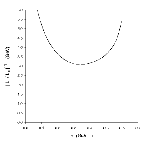
Figure 2: The ratio $\sqrt{\mathcal{L}_{1}/\mathcal{L}_{0}}$ as a function of $\tau$ for central values of the QCD parameters.

As illustrated in Figures 3 and 4, the rise past the minimum in Figure 2 is actually a manifestation of a zero which occurs in $\mathcal{L}_{0}(\tau)$ prior to the first zero of $\mathcal{L}_{1}(\tau)$, resulting in a singularity of the ratio (27). Negative values of $\mathcal{L}_{k}(\tau)$ are inconsistent with (5) and positivity of the spectral function $\rho(t)$. This unphysical behaviour of the sum-rules can be traced to the instanton contributions in the low-energy (large $\tau$) regime.

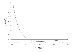
Figure 3: The sum-rule $\mathcal{L}_{0}\left(\tau\right)=\lim_{s_{0}\to\infty}R_{0}\left(\tau,s_{0}\right)$ as a function of $\tau$. Central values of the QCD parameters have been used.

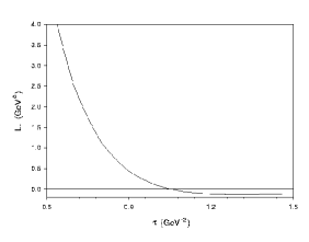
Figure 4: The sum-rule $\mathcal{L}_{1}\left(\tau\right)=\lim_{s_{0}\to\infty}R_{1}\left(\tau,s_{0}\right)$ as a function of $\tau$. Central values of the QCD parameters have been used.

The unphysical low-energy behaviour of the sum-rules does not necessarily invalidate the bounds obtained from Figure 2 because the minimum occurs in the perturbative (high-energy, low $\tau$) regime, but it does present difficulties in the extraction of an optimized mass estimate. Within the single narrow resonance model, (26) results in

$$\frac{R_{1}\left(\tau,s_{0}\right)}{R_{0}\left(\tau,s_{0}\right)}=M^{2}\quad.$$ (28)

In a typical sum-rule analysis [17], one decreases $s_{0}$ until a stable (i.e. nearly $\tau$-independent) ratio (28) is obtained. Figure 5 shows that the ratio does stabilize at approximately $2.7\,{\rm GeV}$, but the small $\tau$ values associated with this stability region are problematic because dominance of the lightest resonance cannot be assured and uncertainties from the continuum approximation become significant. However, because (27) has general validity beyond these approximations, the $M<3.1\,{\rm GeV}$ bound remains valid.

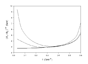
Figure 5: Sum-rule ratios $\sqrt{R_{1}\left(\tau,s_{0}\right)/R_{0}\left(\tau,s_{0}\right)}$ ranging from $s_{0}=\infty$ (i.e. $\sqrt{\mathcal{L}_{1}/\mathcal{L}_{0}}$) in the top curve to $s_{0}=8\,{\rm GeV^{2}}$ in the bottom curve. Central values of the QCD parameters have been used.

Thus instanton effects prevent the extraction of a reliable optimized Laplace sum-rule mass prediction for pseudoscalar gluonium, a difficulty that has also been observed in the configuration-space instanton analysis [24]. It is interesting that the resonance signal in each case is exponential decay associated with the resonance mass combined with $\tau$ in the Laplace sum-rules (26) or with Euclideanized time in the configuration-space approach [24]. The next Section will review the formulation of Gaussian sum-rules which will be seen to provide a fundamentally-different weighting of the hadronic spectral function and QCD contributions, obviating the problems associated with an optimization of the Laplace sum-rule analysis.

4 Gaussian Sum-Rules for Pseudoscalar Gluonium

The simplest Gaussian sum-rule (GSR) [29]

$$G\left(\hat{s},\tau\right)=\frac{1}{\pi}\int\limits_{t_{0}}^{\infty}\frac{1}{\sqrt{4\pi\tau}}\exp{\left(-\frac{\left(t-\hat{s}\right)^{2}}{4\tau}\right)}\,\rho(t)\,\mathrm{d}t\quad,\quad\tau>0$$ (29)

relates the QCD prediction on the left-hand side of (29) to the hadronic spectral function $\rho(t)$ smeared over the energy range $\hat{s}-2\sqrt{\tau}\lesssim t\lesssim\hat{s}+2\sqrt{\tau}$, representing an energy interval for quark-hadron duality. An interesting aspect of the GSR is that the duality interval is actually constrained by QCD. A lower bound on this duality scale $\tau$ necessarily exists because the QCD prediction has renormalization-group properties that reference running quantities the the energy scale $\nu^{2}=\sqrt{\tau}$ [29, 30]. Thus it is not possible to achieve the formal $\tau\to 0$ limit where complete knowledge of the spectral function could be obtained via

$$\lim_{\tau\to 0}G\left(\hat{s},\tau\right)=\frac{1}{\pi}\rho\left(\hat{s}\right)\quad,\quad\hat{s}>t_{0}\quad.$$ (30)

However, there is no theoretical constraint on the quantity $\hat{s}$ representing the peak of the Gaussian kernel appearing in (29). Thus the $\hat{s}$ dependence of the QCD prediction $G\left(\hat{s},\tau\right)$ probes the behaviour of the smeared spectral function, reproducing the essential features of the spectral function. In particular, as $\hat{s}$ passes through $t$ values corresponding to resonance peaks, the Gaussian kernel in (29) reaches its maximum value, implying that Gaussian sum-rules weight excited and ground states equally.

The QCD prediction for the GSR is obtained from the correlation function through

$$G(\hat{s},\tau)\equiv\sqrt{\frac{\tau}{\pi}}\mathcal{B}\left\{\frac{\Pi\left(-\hat{s}-i\Delta\right)-\Pi\left(-\hat{s}+i\Delta\right)}{i\Delta}\right\}\quad,$$ (31)

where the Borel transform $\mathcal{B}$ has been redefined as

$$\mathcal{B}\equiv\lim_{\stackrel{{\scriptstyle N,\Delta^{2}\rightarrow\infty}}{{\Delta^{2}/N\equiv 4\tau}}}\frac{(-\Delta^{2})^{N}}{\Gamma(N)}\left(\frac{\mathrm{d}}{\mathrm{d}\Delta^{2}}\right)^{N}\quad.$$ (32)

The GSR (29) then results from combining (31) with the dispersion relation (2) [29].

A connection between Gaussian and finite-energy sum-rules can be established through the diffusion equation satisfied by the GSR

$$\frac{\partial^{2}G\left(\hat{s},\tau\right)}{\partial\hat{s}^{2}}=\frac{\partial G\left(\hat{s},\tau\right)}{\partial\tau}\quad.$$ (33)

In particular, the resonance(s) plus continuum model (6), when $\rho^{{had}}(t)$ is evolved through the diffusion equation (33), only reproduces the QCD prediction at large energies ($\tau$ large) if the resonance and continuum contributions are balanced through the finite-energy sum-rule [29]

$$F\left(s_{0}\right)=\frac{1}{\pi}\int\limits_{t_{0}}^{s_{0}}\rho^{had}(t)\,\mathrm{d}t\quad.$$ (34)

Within the resonance(s) plus continuum model (6), the continuum contribution to the GSR is determined by QCD

$$G^{{cont}}(\hat{s},\tau,s_{0})=\frac{1}{\sqrt{4\pi\tau}}\int_{s_{0}}^{\infty}\exp\left[\frac{-(\hat{s}-t)^{2}}{4\tau}\right]\frac{1}{\pi}{\rm Im}\Pi^{QCD}(t)\d{t}\quad,$$ (35)

and is thus combined with $G_{k}\left(\hat{s},\tau\right)$ to give the total QCD contribution

$$G^{qcd}\left(\hat{s},\tau,s_{0}\right)\equiv G\left(\hat{s},\tau\right)-G^{{cont}}\left(\hat{s},\tau,s_{0}\right)\quad,$$ (36)

resulting in the final relation between the QCD and hadronic sides of the GSR.

$$G^{qcd}\left(\hat{s},\tau,s_{0}\right)=\int_{t_{0}}^{\infty}\exp\left[\frac{-(\hat{s}-t)^{2}}{4\tau}\right]\frac{1}{\pi}\rho^{had}(t)\d{t}\quad.$$ (37)

Comparison of (37) and (8) reveals that the GSR provides a fundamentally different weighting of the hadronic spectral function than the Laplace sum-rule. In particular, the Laplace sum-rules always emphasize the low-energy region, while this aspect is controlled in the GSR by the parameter $\hat{s}$.

The expression for the QCD prediction for the pseudoscalar gluonium GSR can then be constructed using the results of [16].

$$\begin{split}G^{qcd}(\hat{s},\tau,s_{0})&=-\frac{1}{\sqrt{4\pi\tau}}\int_{0}^{s_{0}}\!\!t^{2}\d{t}\exp\left[\frac{-(\hat{s}-t)^{2}}{4\tau}\right]\Biggl{[}(a_{0}-\pi^{2}a_{2})+2a_{1}\log\left(\frac{t}{\nu^{2}}\right)\Biggr{.}\\ &\phantom{-\frac{1}{\sqrt{4\pi\tau}}\int_{0}^{s_{0}}t^{2}\d{t}\exp\left[\frac{-(\hat{s}-t)^{2}}{4\tau}\right]}\qquad\Biggl{.}+3a_{2}\log^{2}\left(\frac{t}{\nu^{2}}\right)\Biggr{]}\\ &-\frac{1}{\sqrt{4\pi\tau}}b_{1}\langle\alpha G^{2}\rangle\int_{0}^{s_{0}}\exp\left[\frac{-(\hat{s}-t)^{2}}{4\tau}\right]\d{t}\\ &+\frac{1}{\sqrt{4\pi\tau}}\exp\left(\frac{-\hat{s}^{2}}{4\tau}\right)\left[c_{0}\left\langle{\mathcal{O}}_{6}\right\rangle-\frac{d_{0}\hat{s}}{2\tau}\left\langle{\mathcal{O}}_{8}\right\rangle\right]\\ &+\frac{16\pi^{3}}{\sqrt{4\pi\tau}}\int\!\!\d{n}(\rho)\rho^{4}\int_{0}^{s_{0}}t^{2}\exp\left[\frac{-(\hat{s}-t)^{2}}{4\tau}\right]J_{2}\left(\rho\sqrt{t}\right)Y_{2}\left(\rho\sqrt{t}\right)\d{t}\end{split}$$ (38)

As mentioned earlier, renormalization-group improvement necessitates the replacement $\nu^{2}=\sqrt{\tau}$ in (38) [29, 30]. As with the Laplace sum-rules, the one-loop term provides the leading $\left\langle\alpha G^{2}\right\rangle$ contribution to the GSR. For the dimension-six and -eight non-perturbative QCD condensate contributions in (38), it is easily seen that the non-perturbative corrections are exponentially suppressed for large $\hat{s}$. Since $\hat{s}$ represents the location of the Gaussian peak on the phenomenological side of the sum-rule, the non-perturbative corrections are most important in the low-energy region, as anticipated by the role of QCD condensates in relation to the vacuum properties of QCD. This explicit low-energy role of the QCD condensates clearly exhibited for the Gaussian sum-rules is obscured in the Laplace sum-rules.

Integrating both sides of (37) reveals that the overall normalization of the above equation is related to the finite-energy sum-rule [30]

$$\int\limits_{-\infty}^{\infty}G^{qcd}(\hat{s},\tau,s_{0})\d{\hat{s}}=\frac{1}{\pi}\int\limits_{t_{0}}^{\infty}\rho^{{had}}(t)\d{t}\quad.$$ (39)

Thus the diffusion equation analysis [16] relates the normalization of the GSR to the finite-energy sum-rules. Information independent of this relation is thus extracted from the normalized GSR [30]

$$N^{qcd}(\hat{s},\tau,s_{0})\equiv\frac{G^{qcd}\left(\hat{s},\tau,s_{0}\right)}{m_{0}\left(\tau,s_{0}\right)}$$ (40)

$$m_{n}(\tau,s_{0})=\int\limits_{-\infty}^{\infty}\hat{s}^{n}G^{qcd}\left(\hat{s},\tau,s_{0}\right)\d{\hat{s}}\quad,\quad n=0,1,2,\ldots\quad,$$ (41)

which is related to the hadronic spectral function via

$$N^{qcd}\left(\hat{s},\tau,s_{0}\right)=\frac{\int\limits_{t_{0}}^{\infty}\exp\left[\frac{-(\hat{s}-t)^{2}}{4\tau}\right]\rho^{{had}}(t)\d{t}}{\sqrt{4\pi\tau}\int\limits_{t_{0}}^{\infty}\rho^{{had}}(t)\,\d t}\quad.$$ (42)

5 Gaussian Sum-Rule Analysis of Pseudoscalar Gluonium

The techniques for analyzing the GSRs were initially developed in [16, 30]. In the single narrow resonance model, the normalized GSR (42) becomes

$$N^{qcd}\left(\hat{s},\tau,s_{0}\right)=\frac{1}{\sqrt{4\pi\tau}}\exp\left[-\frac{(\hat{s}-M^{2})^{2}}{4\tau}\right]\quad.$$ (43)

Deviations from the narrow-width limit are proportional to $M^{2}\Gamma^{2}/\tau$, so this narrow-width model may be a good numerical approximation. Phenomenological analysis of the single narrow resonance model proceeds from the observation that, as a function of $\hat{s}$, the phenomenological side of (43) has a maximum value (peak) at $\hat{s}=M^{2}$ independent of the value of $\tau$. The value of $s_{0}$ is then optimized by minimizing the $\tau$ dependence of the $\hat{s}$ peak position of the QCD prediction, and the resulting $\tau$-averaged $\hat{s}$ peak position leads to a prediction of the resonance mass [30].

For the central values of the QCD parameters, minimizing the $\hat{s}$ peak motion in the region $2\,{\rm GeV^{4}}<\tau<4\,{\rm GeV^{4}}$ results in $M=2.70\,{\rm GeV}$ for $\sqrt{s_{0}}=3.3\,{\rm GeV}$, which is remarkably similar to the mass scale resulting from the Laplace sum-rule stability analysis in Figure 5. Although an optimized Laplace sum-rule analysis was not possible, a consistent scenario is emerging from the two approaches.

Figure 6 compares the theoretical and phenomenological sides of the normalized GSR (42). It is evident from this comparison that the single narrow resonance model is an inadequate description of the spectral function predicted by QCD. Figure 6 also reveals a region of small $\hat{s}$ where the theoretical GSR is negative, inconsistent with a positive spectral function through (42). This effect can again be traced to the instanton contributions, and since $\hat{s}$ corresponds to the peak of the Gaussian kernel, it is clear that this is a low-energy non-perturbative effect that is safely isolated from the peak of the theoretical contribution which enters the optimization analysis.

By construction, all the curves in Figure 6 are normalized to unit area, so the QCD contributions which underestimate the peak are necessarily broader than those of the single narrow resonance model. In particular, moment combinations (41) associated with (43) result in

$$\frac{m_{2}}{m_{0}}-\left(\frac{m_{1}}{m_{0}}\right)^{2}=2\tau\quad.$$ (44)

Thus the narrow-resonance width of $2\tau$ is insufficient to provide agreement with QCD, indicative of distributed resonance strength that can be resolved by the GSR.

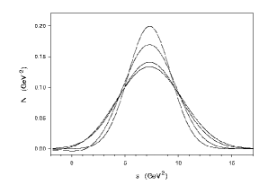
Figure 6: Comparison of the QCD and single narrow resonance model contributions to the normalized GSRs as a function of $\hat{s}$ for the optimized parameters $M=2.70\,{\rm GeV}$ and $\sqrt{s_{0}}=3.3\,{\rm GeV}$ for $\tau=2\,{\rm GeV^{4}}$ (upper pair of curves) and for $\tau=4\,{\rm GeV^{4}}$ (lower pair of curves). In each case, the peak of the theoretical (QCD) prediction lies below that of the single-resonance model.

A simple toy model that illustrates the effect of resonance widths in the broadening of the phenomenological side of the normalized GSR is a unit-area “square pulse” which could describe a broad structureless feature of the spectral function

$$\frac{1}{\pi}\rho^{{had}}(t)=\frac{1}{2M\Gamma}\left[\theta\left(t-M^{2}+M\Gamma\right)-\theta\left(t-M^{2}-M\Gamma\right)\right]\quad,$$ (45)

which leads to the following normalized Gaussian sum-rule [16]

$$N^{qcd}\left(\hat{s},\tau,s_{0}\right)=\frac{1}{4M\Gamma}\left[{\rm erf}\left(\frac{\hat{s}-M^{2}+M\Gamma}{2\sqrt{\tau}}\right)-{\rm erf}\left(\frac{\hat{s}-M^{2}-M\Gamma}{2\sqrt{\tau}}\right)\right]\quad.$$ (46)

The second-order moment combinations resulting from this sum-rule are [16]

$$\frac{m_{2}}{m_{0}}-\left(\frac{m_{1}}{m_{0}}\right)^{2}=2\tau+\frac{1}{3}M^{2}\Gamma^{2}\quad,$$ (47)

and hence resonance widths broaden the phenomenological side of the normalized GSR as would be expected intuitively.

For detailed analysis, the following Gaussian resonance and a skewed-Gaussian resonance models will be employed since they are numerically simpler to analyze than a Breit-Wigner resonance shape.

$$\rho(t)\sim\exp{\left[-\frac{\left(t-M^{2}\right)^{2}}{2\gamma^{2}}\right]}$$ (48)

$$\rho(t)\sim t^{2}\exp{\left[-\frac{\left(t-M^{2}\right)^{2}}{2\gamma^{2}}\right]}$$ (49)

The quantity $\gamma$ can be related to a Breit-Wigner width $\Gamma$ by equating the half-widths, resulting in $\Gamma=\sqrt{2\log 2}\,\gamma/M$. For the Gaussian model, the resulting normalized GSR is [16]

$$N^{qcd}\left(\hat{s},\tau,s_{0}\right)=\frac{1+\text{erf}\left(\frac{\hat{s}\gamma^{2}+2M^{2}\tau}{2\gamma\sqrt{\tau}\sqrt{\gamma^{2}+2\tau}}\right)}{\sqrt{2\pi}\sqrt{\gamma^{2}+2\tau}\left[1+\text{erf}\left(\frac{M^{2}}{\sqrt{2}{\gamma}}\right)\right]}\exp\left[-\frac{\left(\hat{s}-M^{2}\right)^{2}}{2\left(\gamma^{2}+2\tau\right)}\right]\quad.$$ (50)

For the skewed Gaussian model, the resulting normalized GSR is

$$\begin{split}\frac{N^{qcd}\left(\hat{s},\tau,s_{0}\right)}{A}=&\exp\left[-\frac{\left(\hat{s}-M^{2}\right)^{2}}{2\left(\gamma^{2}+2\tau\right)}\right]\left[1+\text{erf}\left(\frac{\hat{s}\gamma^{2}+2M^{2}\tau}{2\gamma\sqrt{\tau}\sqrt{\gamma^{2}+2\tau}}\right)\right]\\ &\times\sqrt{\pi}\left[\hat{s}^{2}\gamma^{4}+4\hat{s}\gamma^{2}\tau M^{2}+4\tau^{2}M^{4}+2\tau\gamma^{4}+4\tau^{2}\gamma^{2}\right]\\ &+2\gamma\left(\hat{s}\gamma^{2}+2\tau M^{2}\right)\sqrt{\tau\left(\gamma^{2}+2\tau\right)}\exp{\left[-\frac{\hat{s}^{2}\gamma^{2}+2\tau M^{4}}{4\tau\gamma^{2}}\right]}\end{split}$$ (51)

where

$$A=\frac{\frac{\gamma}{2\sqrt{\pi}\left(\gamma^{2}+2\tau\right)^{5/2}}}{M^{2}\gamma^{2}\exp{\left(-\frac{M^{4}}{2\gamma^{2}}\right)}+\sqrt{\frac{\pi}{2}}\left(M^{4}\gamma+\gamma^{3}\right)\left[1+\text{erf}\left(\frac{M^{2}}{\gamma\sqrt{2}}\right)\right]}~{}.$$ (52)

The inclusion of resonance widths implies that the $\hat{s}$ peak position of the phenomenological side of the sum-rules can develop $\tau$ dependence, complicating the optimization of $s_{0}$. The direct approach of determining all parameters from the best fit between the $\hat{s}$ dependence of the two sides of (50) and (51) over the range $2\,{\rm GeV^{4}}<\tau<4\,{\rm GeV^{4}}$ is facilitated by an initial estimate of $s_{0}$. An effective estimate of the optimized $s_{0}$ is obtained from the (approximate) $\tau$ dependence of the $\hat{s}$ peak which has the general behaviour [16, 30]

$$\hat{s}_{peak}\left(\tau,s_{0}\right)=a+\frac{b}{\tau}+\frac{c}{\tau^{2}}\quad.$$ (53)

Analysis of how the $\hat{s}$ peak “drifts” with $\tau$ in comparison with the behaviour (53) provides an estimate of $s_{0}$ which is found to be surprisingly close to the true fitted value, facilitating numerical analysis of the multi-dimensional fit.

For the central values of the QCD parameters, the resulting optimized parameters are $M=2.7\,{\rm GeV}$, $\Gamma=0.50\,{\rm GeV}$ in the Gaussian resonance model, and $M=2.6\,{\rm GeV}$, $\Gamma=0.53\,{\rm GeV}$ in the skewed Gaussian resonance model, with $\sqrt{s_{0}}=3.2\,{\rm GeV}$ in each case. The agreement between the QCD and phenomenological sides of the normalized GSR for the skewed Gaussian model is shown in Figure 7. Comparison of Figures 6 and 7 (which have identical scales) reveals that inclusion of a resonance width provides a significant improvement in the agreement between the QCD and phenomenological sides of the sum-rule without a significant change in the predicted resonance mass.

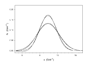
Figure 7: Comparison of the QCD and skewed-Gaussian resonance model contributions to the normalized GSR as a function of $\hat{s}$ for the optimized parameters $M=2.6\,{\rm GeV}$, $\Gamma=0.53\,{\rm GeV}$, and $\sqrt{s_{0}}=3.2\,{\rm GeV}$ for $\tau=2\,{\rm GeV^{4}}$ (upper pair of curves) and for $\tau=4\,{\rm GeV^{4}}$ (lower pair of curves). For the upper pair of curves the peak of the theoretical (QCD) prediction lies above that of the single-resonance model, but the situation is reversed for the lower pair of curves.

The un-skewed Gaussian resonance model results in an agreement between the QCD and phenomenological sides of the normalized GSR which is qualitatively and quantitatively indistinguishable from Figure 7. Unlike the single narrow resonance model where theory consistently underestimated the phenomenological peak, there is no evident pattern in the disagreement between QCD and the skewed-Gaussian model. It is possible that the slight disagreement that remains between QCD and the phenomenological model can be explained by the low-energy region where $G^{qcd}$ is negative, since this reduces the quantity $m_{0}$ for $\tau=2\,{\rm GeV^{4}}$, and hence raises the value of $N^{qcd}$. Thus there is no clear motivation for considering more complex resonance models.

The effect of varying the QCD instanton parameters by 15% and the gluon condensate within the range (24) in both the Gaussian and skewed-Gaussian models provides a final determination of the mass and width of pseudoscalar gluonium

$$M=(2.65\pm 0.33)\,{\rm GeV}\quad,\quad\Gamma<540\,{\rm MeV}\quad.$$ (54)

An interesting aspect of this analysis is that smaller instanton sizes are essentially consistent with a narrow resonance model.

6 Conclusions

Instanton and higher-loop perturbative effects have been incorporated into the Laplace and Gaussian sum-rules for pseudoscalar gluonium. Although the Gaussian sum-rules are found to be superior to the Laplace sum-rules in obtaining an optimized prediction of the pseudoscalar gluonium properties, the resulting mass scales in each analysis are remarkably consistent, providing corroborating evidence in support of our final mass prediction of $M\approx 2.7\,{\rm GeV}$. Our mass estimate is consistent with the benchmark lattice scalar glueball mass of approximately $1.6\,{\rm GeV}$ and a pseudoscalar to scalar mass ratio of approximately 1.5 [1].

The analysis presented in this paper has not pursued the interesting possibility of mixing between gluonium and quark mesons [31], although in principle any hadronic state that overlaps with the pseudoscalar gluonium interpolating field would be probed by the correlator (1) which underlies our entire analysis.

This possibility of other resonances coupled to the pseudoscalar gluonic current was explored through an extension of the Section 5 analysis to two narrow resonances tends to lead to nearly-degenerate states near $2.7\,{\rm GeV}$, suggesting that the $2.7\,{\rm GeV}$ state is more strongly coupled to the pseudoscalar gluonic operator than other pseudoscalar states such as the $\eta^{\prime}$. This result is not unexpected, since the coupling of the $2.7\,{\rm GeV}$ state $|P\rangle$ to the pseudoscalar gluonic current extracted from the peak value of $G^{qcd}\left(\hat{s},\tau,s_{0}\right)$ with the optimized value of $s_{0}$ is

$$\left|\langle O\left|\alpha G\tilde{G}\right|P\rangle\right|\approx 20\,{\rm GeV^{3}}\quad.$$ (55)

By comparison, the couplings of $\eta,\eta^{\prime}$ to the pseudoscalar gluonic operators are [32]

$$\left|\langle O\left|\alpha G\tilde{G}\right|\eta^{\prime}\rangle\right|\approx 0.9\,{\rm GeV^{3}}~{},~{}\left|\langle O\left|\alpha G\tilde{G}\right|\eta\rangle\right|\approx 0.1\,{\rm GeV^{3}}~{},$$ (56)

and hence the relative strength of the $|\eta^{\prime}\rangle$ compared with $|P\rangle$ obtained from the ratios of the squares of (55) and (56) is approximately 0.2%, and the relative strength of the $|\eta\rangle$ is approximately 0.02%. This result is upheld by a fit of the relative strength of the $\eta^{\prime}$ and a Gaussian resonance to the normalized GSR results in a relative strength of less than 1%. Thus the $2.7\,{\rm GeV}$ state resulting from our analysis appears to be dominantly-coupled to the pseudoscalar gluonic operators.

7 Acknowledgments

Research funding from the Natural Science & Engineering Research Council of Canada (NSERC) is gratefully acknowledged. Ailin Zhang is partly supported by National Natural Science Foundation of China.

References

-
[1]
C. Morningstar and M. Peardon, Phys. Rev. D60 (1999) 034509;
W. Lee and D. Weingarten, Phys. Rev. D61 (2000) 014015. - [2] A. Hart and M. Teper (UKQCD Collaboration), Phys. Rev. D65 (2002) 034502.
- [3] V.A. Novikov, M.A. Shifman, A.I. Vainshtein, and V. I. Zakharov, Nucl. Phys. B165 (1980) 67; ibid. B191 (2001) 301.
-
[4]
M.A. Shifman, Z. Phys. C9 (1981) 347;
P. Pascual and R. Tarrach, Phys. Lett. B113 (1982) 495;
S. Narison, Z. Phys. C26 (1984) 209;
C.A. Dominguez and N. Paver, Z. Phys. C31 (1986) 591;
J. Bordes, V. Gimènez and J.A. Peñarrocha, Phys. Lett. B223 (1989) 251;
J.P. Liu and D. Liu, J. Phys. G19 (1993) 373;
L.S. Kisslinger, J. Gardner and C. Vanderstraeten, Phys. Lett. B410 (1997) 1. -
[5]
K. Senba and M. Tanimoto, Phys. Lett. B105 (1981) 297;
S. Narison, Phys. Lett. B255 (1991) 101. -
[6]
E. Bagan and T.G. Steele, Phys. Lett. B243 (1990) 413;
S. Narison, Nucl. Phys. B509 (1998) 312. - [7] D. Asner, R.B. Mann, J.L. Murison, and T.G. Steele Phys. Lett. B296 (1992) 171.
-
[8]
H. Forkel, Phys. Rev. D64 (2001) 034015;
L.S. Kisslinger and M.B. Johnson, Phys. Lett. B523 (2001) 127. - [9] D. Harnett, T.G. Steele and V. Elias, Nucl. Phys. A686 (2001) 393.
-
[10]
Tao Huang, Hongying Jin and Ailin Zhang, Phys. Rev. D59 (1999) 034026;
S. Narison and G. Veneziano, Int. J. Mod. Phys. A4 (1989) 2751. - [11] E.V. Shuryak, Nucl. Phys. B203 (1982) 116.
-
[12]
T. Barnes, F. Close and S. Monaghan, Nucl. Phys. B198(1982) 380 ;
C.E. Carlson, T. Hansson and C. Peterson, Phys. Rev. D27 (1983) 1556;
N. Isgur, R. Kokoski and J. Paton, Phys. Rev. Lett, 54 (1985) 869;
A. Szczepaniak, E.S. Swanson, C.R. Ji and S.R. Cotanch, Phys. Rev. Lett. 76 (1996) 2011. - [13] Particle Data Group (K. Hagiwara et al ), Phys. Rev. D66 (2002) 010001.
- [14] E. Bagan and T.G. Steele, Phys. Lett. B234 (1990) 135.
-
[15]
A. Belavin, A. Polyakov, A. Schwartz and Y. Tyupkin,
Phys. Lett. B59 (1975) 85;
G. ’t Hooft, Phys. Rev. D14 (1976) 3432;
C.G. Callan, R. Dashen and D. Gross, Phys. Rev. D17 (1978) 2717;
M.A. Shifman, A.I. Vainshtein and V.I. Zakharov, Nucl. Phys. B165 (1980) 45. - [16] D. Harnett and T.G. Steele, Nucl. Phys. A695 (2001) 205.
- [17] M.A. Shifman, A.I. Vainshtein and V.I. Zakharov, Nucl. Phys. B147 (1979) 385, 448.
- [18] K.G. Chetyrkin, B.A. Kniehl and M. Steinhauser, Phys. Rev. Lett. 79 (1997) 353.
- [19] A.L. Kataev, N.V. Krasnikov, A.A. Pivovarov, Nucl. Phys. B198 (1982) 508, Erratum ibid B490 (1997) 505.
- [20] V.A. Novikov, M.A. Shifman, A.I. Vainshtein and V.I. Zakharov, Phys. Lett. B86 (1979) 347.
-
[21]
B.V. Geshkenbein and B.L. Ioffe, Nucl. Phys. B166 (1980) 340;
B.L. Ioffe and A.V. Samsonov, Phys. of Atom. Nucl. 63 (2000) 1527;
T. Schaefer and E.V. Shuryak, Rev. Mod. Phys. 70 (1998) 323. - [22] M. Abramowitz and I.E. Stegun, Mathematical Functions with Formulas, Graphs, and Mathematical Tables (National Bureau of Standards Applied Mathematics Series, Washington) 1972.
- [23] E. Bagan, M.R. Ahmady, V. Elias, T.G. Steele, Z. Phys. C61 (1994) 157.
- [24] T. Schäefer and E.V. Shuryak, Phys. Rev. Lett. 75 (1995) 1707.
- [25] S. Narison and E. de Rafael, Phys. Lett. B103 (1981) 57.
- [26] E.V. Shuryak, Nucl. Phys. B203 (1982) 93.
- [27] E. Bagan, J.I. Latorre, P. Pascual and R. Tarrach, Nucl. Phys. B254 (1985) 555.
- [28] S. Narison, Nucl. Phys. B (Proc. Supp.) 54A (1997) 238.
- [29] R.A. Bertlmann, G. Launer, E. de Rafael, Nucl. Phys. B250 (1985) 61.
- [30] G. Orlandini, T.G. Steele and D. Harnett, Nucl. Phys. A686 (2001) 261.
-
[31]
P. Ball, J.M. Frere and M. Tytgat, Phys. Lett. B365 (1996) 367;
F. De Fazio and M.R. Pennington, JHEP 0007 (2000) 051;
E. Kou, Phys. Rev. D63 (2001) 054027. -
[32]
V.A. Novikov, M.A. Shifman, A.I. Vainshtein, and V. I. Zakharov, Nucl. Phys. B165 (1980) 55;
F. De Fazio, M.R. Pennington, JHEP 0007 (2000) 051.