$D_{s}$ decays into $\phi$ and $f_{0}(980)$ mesons

Abstract

We consider the nonleptonic and semileptonic decays of $D_{s}$-mesons into $\phi$ and $f_{0}(980)$ mesons. QCD sum rules are used to calculate the form factors associated with these decays, and the correspondig decay rates. On the basis of data on $D_{s}^{+}\rightarrow\pi^{+}\pi^{+}\pi^{-}$, which goes dominantly via the transition $D_{s}^{+}\rightarrow\pi^{+}f_{0}(980)$, we conclude that there is space for a sizeable light quark component on $f_{0}(980)$.

I Introduction

The interpretation of the nature of the lightest scalar mesons have been controversial since their first observation over thirty years ago. Due to the complications of the nonperturbative strong interactions there is still no general agreement about their structure. Actually, the observed light scalar states are too numerous PDG to be accomodated in a single $q\bar{q}$ multiplet, and therefore, it has been suggested that some of them escape the quark model interpretation. It is not known whether there is necessarily a glueball among the light scalar, and whether some of the too numerous scalars are multiquark or some meson-meson bound states, or even admixtures of quarks and gluons cloto .

In particular, the structure of the meson $f_{0}(980)$ has been extensively debated. It has been interpreted as an $s\bar{s}$ state torn ; bev ; col , as an four quark $s\bar{s}q\bar{q}$ state jaffe , as a bound state of hadrons wein ; clo1 , and as a result of a process known as hadronic dressing torn ; bev ; faz .

The recently measured relative weight of the reaction $D_{s}^{+}\rightarrow f_{0}(980)\pi^{+}\rightarrow\pi^{+}\pi^{-}\pi^{+}$ Ait01 , may serve as a tool for the estimation of the $s\bar{s}$ component of the meson $f_{0}(980)$. As a matter of fact, if $f_{0}(980)$ has a pure strangeness component ($f_{0}(980)=s\bar{s}$), the dominant $D_{s}^{+}\rightarrow f_{0}(980)\pi^{+}$ decay proceeds via the spectator mechanism, as shown in Fig. 1. However, in the four quark scenario ($f_{0}(980)=s\bar{s}(u\bar{u}+d\bar{d})/2$) the decay $D_{s}^{+}\rightarrow f_{0}(980)\pi^{+}$ is expected to proceed through a much more complicated recombination.

Figure 1: Schematic picture of the spectator mechanism for the decay $D_{s}^{+}\rightarrow f_{0}(980)\pi^{+}$.

Since the spectator mechanism provides a strong production of the $\phi(1020)$ meson in the decay $D_{s}^{+}\rightarrow\phi\pi^{+}$, in this work we consider the ratio

$$R={\Gamma(D_{s}^{+}\rightarrow f_{0}(980)\pi^{+})\over\Gamma(D_{s}^{+}\rightarrow\phi\pi^{+})}\;,$$ (1)

to evaluate the importance of the $s\bar{s}$ component in the $f_{0}(980)$ meson. This same ratio was evaluated in recent calculations by using the spectral integration technique adn , and the constituent quark meson model detc . In both calculations the authors concluded that the $s\bar{s}$ component dominates the $f_{0}(980)$ meson and, therefore, the spectator mechanism dominates the $D_{s}^{+}\rightarrow f_{0}(980)\pi^{+}$ decay. Here we use the QCD sum rules method to evaluate the ratio in Eq. (1), as well as the branching ratios for the nonleptonic $D_{s}^{+}\rightarrow\phi\pi^{+}$ and semileptonic $D_{s}^{+}\rightarrow\phi\ell^{+}\nu_{\ell}$ and $D_{s}^{+}\rightarrow f_{0}(980)\ell^{+}\nu_{\ell}$ decays. The two branching ratios involving the meson $\phi$ will be used to check the reliability of the method, since these two branching ratios are known experimentaly PDG :

$${\cal B}^{exp}(D_{s}^{+}\rightarrow\phi\pi^{+})=(3.6\pm 0.9)\%\;,$$ (2)

$${\cal B}^{exp}(D_{s}^{+}\rightarrow\phi\ell^{+}\nu_{\ell})=(2.0\pm 0.5)\%\;.$$ (3)

II Decay widths

The decay width of the nonleptonic process $D_{s}^{+}\rightarrow M\pi^{+}$, where $M$ stands for the $\phi$ or $f_{0}(980)$ mesons, is given by:

$$\Gamma(D_{s}^{+}\rightarrow M\pi^{+})={1\over 16\pi m_{D_{s}}^{3}}|{\cal M}|^{2}\sqrt{\lambda(m_{D_{s}}^{2},m_{M}^{2},m_{\pi}^{2})}\;,$$ (4)

with $\lambda(x,y,z)=x^{2}+y^{2}+z^{2}-2xy-2xz-2yz$. The QCD factorization formula (in the limit $m_{\pi}^{2}\rightarrow 0$) gives for $f_{0}(980)$:

$$|{\cal M}(D_{s}^{+}\rightarrow f_{0}(980)\pi^{+})|^{2}={G_{F}^{2}\over 2}|V_{cs}|^{2}|V_{ud}|^{2}\left(c_{1}+{c_{2}\over 3}\right)^{2}f_{\pi}^{2}(m_{D_{s}}^{2}-m_{f_{0}}^{2})^{2}f_{+}^{2}(0),$$ (5)

where $f_{+}$ is the $D_{s}\rightarrow f_{0}(980)$ form factor defined as

$$\langle f_{0}(p^{\prime})|\bar{s}\gamma_{\mu}(1-\gamma_{5})c|D_{s}(p)\rangle=i(f_{+}(t)(p+p^{\prime})_{\mu}+f_{-}(t)q_{\mu}),$$ (6)

with $t=q^{2}$ and $q=p-p^{\prime}$. And for $\phi$ we have

$$|{\cal M}(D_{s}^{+}\rightarrow\phi\pi^{+})|^{2} = {G_{F}^{2}\over 8m_{\phi}^{2}}|V_{cs}|^{2}|V_{ud}|^{2}\left(c_{1}+{c_{2}\over 3}\right)^{2}f_{\pi}^{2}\lambda(m_{D_{s}}^{2},m_{\phi}^{2},m_{\pi}^{2})[(m_{D_{s}}+m_{\phi})A_{1}(0)$$ (7)

$$- (m_{D_{s}}-m_{\phi})A_{2}(0)]^{2},$$

where $A_{1}$ and $A_{2}$ are $D_{s}\rightarrow\phi$ form factors defined as bbd91

$$\langle\phi(p^{\prime})|\bar{s}\gamma_{\mu}(1-\gamma_{5})c|D_{s}(p)\rangle = -i(m_{D_{s}}+m_{\phi})A_{1}(t)\epsilon^{\phi}_{\mu}+i{A_{2}(t)\over m_{D_{s}}+m_{\phi}}\epsilon^{\phi}.p(p+p^{\prime})_{\mu}$$ (8)

$$+ i{A_{3}(t)\over m_{D_{s}}+m_{\phi}}\epsilon^{\phi}.p~{}q_{\mu}+{2V(t)\over m_{D_{s}}+m_{\phi}}\epsilon_{\mu}^{\nu\rho\sigma}\epsilon^{\phi}_{\nu}p_{\rho}p^{\prime}_{\sigma}.$$

In Eqs. (5) and (7) the coefficients $c_{1}$ and $c_{2}$ are the Wilson coefficients entering the effective weak Hamiltonian evaluated at the normalization scale $\mu$ bubu :

$$H_{W}={G_{F}\over\sqrt{2}}V_{cs}V^{*}_{ud}\left[\left(c_{1}(\mu)+{c_{2}(\mu)\over 3}\right)O_{1}+...\right],$$ (9)

with $O_{1}=(\bar{u}\gamma_{\mu}(1-\gamma_{5})d)(\bar{s}\gamma^{\mu}(1-\gamma_{5})c)$. Therefore, in calculating the ratio in Eq. (1) we are free from the uncertainties in the Wilson coefficients and in the CKM transition elements.

In the case of the semileptonic decays $D_{s}^{+}\rightarrow M\ell^{+}\nu_{\ell}$ the differential decay rates are given by

$$\frac{d\Gamma}{dt}=\frac{G_{F}^{2}|V_{cs}|^{2}}{192\pi^{3}m_{D_{s}}^{3}}\lambda^{3/2}(m_{D_{s}}^{2},m_{f_{0}}^{2},t)f_{+}^{2}(t)\;,$$ (10)

for $D_{s}^{+}\rightarrow f_{0}(980)\ell^{+}\nu_{\ell}$. The decay rate for the decay $D_{s}^{+}\rightarrow\phi\ell^{+}\nu_{\ell}$ is written in terms of the helicity amplitudes

$$H_{\pm}(t)=(m_{D_{s}}+m_{\phi})A_{1}(t)\mp{\lambda^{1/2}(m_{D_{s}}^{2},m_{\phi}^{2},t)\over m_{D_{s}}+m_{\phi}}V(t)\;,$$ (11)

$$H_{0}(t)={1\over 2m_{\phi}\sqrt{t}}\left((m_{D_{s}}^{2}-m_{\phi}^{2}-t)(m_{D_{s}}+m_{\phi})A_{1}(t)-{\lambda(m_{D_{s}}^{2},m_{\phi}^{2},t)\over m_{D_{s}}+m_{\phi}}A_{2}(t)\right)\;,$$ (12)

so that

$$\frac{d\Gamma_{\pm}}{dt}=\frac{G_{F}^{2}|V_{cs}|^{2}}{192\pi^{3}m_{D_{s}}^{3}}t\lambda^{1/2}(m_{D_{s}}^{2},m_{f_{0}}^{2},t)|H_{\pm}(t)|^{2}\;,$$ (13)

$$\frac{d\Gamma_{L}}{dt}=\frac{G_{F}^{2}|V_{cs}|^{2}}{192\pi^{3}m_{D_{s}}^{3}}t\lambda^{1/2}(m_{D_{s}}^{2},m_{f_{0}}^{2},t)|H_{0}(t)|^{2}\;,$$ (14)

$$\frac{d\Gamma_{T}}{dt}=\frac{d}{dt}(\Gamma_{+}+\Gamma_{-}),\;\;\;\;\frac{d\Gamma}{dt}=\frac{d}{dt}(\Gamma_{L}+\Gamma_{T})\;.$$ (15)

III Sum rules

The $D_{s}^{+}$ meson in the initial state is interpolated by the pseudoscalar current

$$j_{D_{s}}(x)=\bar{s}(x)i\gamma_{5}c(x)\;,$$ (16)

where $c$ and $s$ are the fields of the charmed and strange quark respectively. Summation over spinor and colour indices being understood but not indicated explicitly. The final hadronic state $M$ is interpolated by the current

$$j_{M}(x)=\bar{s}(x)\Gamma_{M}s(x)\;,$$ (17)

where

$$\begin{array}[]{c}\Gamma_{M}=\end{array}\left\{\begin{array}[]{c}1\mbox{ for }M=f_{0}(980)\\ \gamma_{\alpha}\mbox{ for }M=\phi\end{array}\right.$$ (18)

Using the QCD sum rule technique svz , the form factors in Eqs. (6) and (8) can be evaluated from the time ordered product of the two interpolating fields in Eqs. (16) and (17) and the weak current $j^{W}_{\mu}=\bar{s}\gamma_{\mu}(1-\gamma_{5})c$

$$T_{\mu M}(p,p^{\prime})=i\int d^{4}xd^{4}y\,\langle 0|{\rm T}[j_{M}(x)j^{W}_{\mu}(y)j_{D_{s}}^{\dagger}(0)]|0\rangle e^{i(p^{\prime}.x-q.y)}\;.$$ (19)

In order to evaluate the phenomenological side we insert intermediate states for $D_{s}$ and $M$, we use the definitions in Eqs. (6) and (8), and obtain the following relations

$$T_{\mu}^{phen}(p,p^{\prime}) = m_{f_{0}}f_{f_{0}}{m_{D_{s}}^{2}f_{D_{s}}\over m_{c}+m_{s}}~{}{f_{+}(t)(p+p^{\prime})_{\mu}+f_{-}(t)~{}q_{\mu}\over(p^{2}-m_{D_{s}}^{2})({p^{\prime}}^{2}-m_{f_{0}}^{2})}$$ (20)

$$+ \mbox{ contributions of higher resonances}\;,$$

for $f_{0}(980)$, and

$$T_{\mu\alpha}^{phen}(p,p^{\prime}) = m_{\phi}f_{\phi}{m_{D_{s}}^{2}f_{D_{s}}\over m_{c}+m_{s}}{1\over(p^{2}-m_{D_{s}}^{2})({p^{\prime}}^{2}-m_{\phi}^{2})}\bigg{(}-(m_{D_{s}}+m_{\phi})A_{1}(t)g_{\mu\alpha}$$ (21)

$$+ {A_{2}(t)\over(m_{D_{s}}+m_{\phi})}(p+p^{\prime})_{\mu}~{}p_{\alpha}-2i{V(t)\over(m_{D_{s}}+m_{\phi})}\epsilon_{\mu\alpha\rho\sigma}~{}p_{\rho}p^{\prime}_{\sigma}$$

$$+ \cdots\bigg{)}+\mbox{ contributions of higher resonances}\;,$$

for $\phi$, where we have shown only the structures important for the evaluation of the form factors $A_{1},~{}A_{2}$ and $V$.

In the above equations the coupling of the $f_{0}(980)$ to the scalar current $j_{s}=\bar{s}s$, was parametrized in terms of the constant $f_{f_{0}}$ as:

$$\langle 0|\bar{s}s|f_{0}\rangle=m_{f_{0}}~{}f_{f_{0}}\;,$$ (22)

and we have used the standard definitions of the couplings of $D_{s}$ and $\phi$ with the corresponding currents:

$$\langle 0|j_{D_{s}}|D_{s}\rangle={m_{D_{s}}^{2}f_{D_{s}}\over m_{c}+m_{s}}\;,$$ (23)

$$\langle 0|\bar{s}\gamma_{\alpha}s|\phi\rangle=m_{\phi}~{}f_{\phi}\epsilon_{\alpha}\;,$$ (24)

The three-point function Eq.(19) can be evaluated by perturbative QCD if the external momenta are in the deep Euclidean region

$$p\ll(m_{c}+m_{s})^{2},~{}~{}~{}{p^{\prime}}^{2}\ll 4m_{s}^{2},~{}~{}~{}t\ll(m_{c}+m_{s})^{2}\;.$$ (25)

In order to approach the not-so-deep-Euclidean region and to get more information on the nearest physical singularities, nonperturbative power corrections are added to the perturbative contribution. In practice, only the first few condensates contribute significantly, the most important ones being the 3-dimension, $\langle\bar{s}s\rangle$, and the 5-dimension, $\langle\bar{s}g_{s}\sigma.Gs\rangle$, condensates. For each invariant structure, $i$, we can write

$$T^{theor}_{i}(p^{2},{p^{\prime}}^{2},t) = {-1\over 4\pi^{2}}\int_{(m_{c}+m_{s})^{2}}^{\infty}ds\int_{4m_{s}^{2}}^{\infty}du\,\frac{\rho_{i}(s,u,t)}{(s-p^{2})(u-{p^{\prime}}^{2})}$$ (26)

$$+ T^{D=3}_{i}\langle\bar{s}s\rangle+T^{D=5}_{i}\langle\bar{s}g_{s}\sigma.Gs\rangle+\cdots\;.$$

The perturbative contribution is contained in the double discontinuity $\rho_{i}$.

In order to suppress the condensates of higher dimension and at the same time reduce the influence of higher resonances, the series in Eq. (26) is Borel improved, leading to the mapping

$$f(p^{2})\to\hat{f}(M^{2}),~{}~{}~{}~{}~{}\frac{1}{(p^{2}-m^{2})^{n}}\to\frac{(-1)^{n}}{(n-1)!}\frac{e^{-m^{2}/M^{2}}}{(M^{2})^{n}}\;.$$ (27)

Furthermore, we make the usual assumption that the contributions of higher resonances are well approximated by the perturbative expression

$${-1\over 4\pi^{2}}\int_{s_{0}}^{\infty}ds\int_{u_{0}}^{\infty}du\,\frac{\rho_{i}(s,u,t)}{(s-p^{2})(u-{p^{\prime}}^{2})}$$ (28)

with appropriate continuum thresholds $s_{0}$ and $u_{0}$. By equating the Borel transforms of the phenomenological expression for each invariant structure in Eqs.(20), (21) and that of the “theoretical expression”, Eq. (26), we obtain the sum rules for the form factors (at the order $m_{s}$):

$$C_{f_{0}}e^{-m_{D_{s}}^{2}/M^{2}}e^{-m_{f_{0}}^{2}/{M^{\prime}}^{2}}f_{+}(t)={-1\over 4\pi^{2}}\int_{(m_{c}+ms)^{2}}^{s_{0}}ds\int_{0}^{u_{0}}du\left[e^{-s/M^{2}}e^{-u/{M^{\prime}}^{2}}\rho_{+}(s,u,t)\right]$$ (29)

$$+ {\langle\bar{s}s\rangle\over 2}e^{-m_{c}^{2}/M^{2}}\left[-m_{c}+2m_{s}+{m_{c}^{2}m_{s}\over 2M^{2}}\right]+\langle\bar{s}g_{s}\sigma.Gs\rangle e^{-m_{c}^{2}/M^{2}}\left[{m_{c}^{2}(m_{c}-m_{s})\over 8M^{4}}-{2m_{c}-m_{s}\over 6M^{2}}\right.$$

$$+ \left.{m_{c}^{2}(4m_{c}-3m_{s})-2t(m_{c}-m_{s})\over 24M^{2}{M^{\prime}}^{2}}-{m_{c}-2m_{s}\over 6{M^{\prime}}^{2}}+{m_{c}^{2}m_{s}-2t(m_{c}-m_{s})\over 24M^{2}{M^{\prime}}^{2}}\right],$$

$$C_{\phi}(m_{D_{s}}+m_{\phi})^{2}e^{-m_{D_{s}}^{2}/M^{2}}e^{-m_{\phi}^{2}/{M^{\prime}}^{2}}A_{1}(t)={-1\over 4\pi^{2}}\int_{(m_{c}+ms)^{2}}^{s_{0}}ds\int_{0}^{u_{0}}du\left[e^{-s/M^{2}}e^{-u/{M^{\prime}}^{2}}\right.$$ (30)

$$\times \left.\rho_{1}(s,u,t)\right]+{\langle\bar{s}s\rangle\over 2}e^{-m_{c}^{2}/M^{2}}\left[t-m_{c}^{2}-{5\over 2}m_{c}m_{s}-{m_{c}m_{s}\over 2M^{2}}(t-m_{c}^{2})\right]$$

$$+ \langle\bar{s}g_{s}\sigma.Gs\rangle e^{-m_{c}^{2}/M^{2}}\left[-{1\over 6}+{m_{c}^{2}(m_{c}^{2}+2m_{c}m_{s}-t)\over 8M^{4}}-{2m_{c}^{2}+3m_{c}m_{s}-2t\over 12{M^{\prime}}^{2}}\right]$$

$$- \left.{3m_{c}^{2}+9m_{c}m_{s}-4t\over 12M^{2}}+{m_{c}(2m_{c}^{3}+3m_{c}m_{s}+tm_{s})/2-t(2m_{c}^{2}+3m_{c}m_{s}/2-2t)\over 6M^{2}{M^{\prime}}^{2}}\right],$$

$$C_{\phi}e^{-m_{D_{s}}^{2}/M^{2}}e^{-m_{\phi}^{2}/{M^{\prime}}^{2}}A_{2}(t) = {-1\over 4\pi^{2}}\int_{(m_{c}+ms)^{2}}^{s_{0}}ds\int_{0}^{u_{0}}du\left[e^{-s/M^{2}}e^{-u/{M^{\prime}}^{2}}\rho_{2}(s,u,t)\right]$$ (31)

$$+ {\langle\bar{s}s\rangle\over 2}e^{-m_{c}^{2}/M^{2}}\left(1-{m_{c}m_{s}\over 2M^{2}}\right)-\langle\bar{s}g_{s}\sigma.Gs\rangle e^{-m_{c}^{2}/M^{2}}$$

$$\times \left[{1\over 6M^{2}}+{m_{c}^{2}\over 8M^{4}}+{2m_{c}^{2}-m_{c}m_{s}-2t\over 12M^{2}{M^{\prime}}^{2}}\right],$$

and

$$-2C_{\phi}e^{-m_{D_{s}}^{2}/M^{2}}e^{-m_{\phi}^{2}/{M^{\prime}}^{2}}V(t) = {-1\over 4\pi^{2}}\int_{(m_{c}+ms)^{2}}^{s_{0}}ds\int_{0}^{u_{0}}du\left[e^{-s/M^{2}}e^{-u/{M^{\prime}}^{2}}\rho_{V}(s,u,t)\right]$$ (32)

$$+ {\langle\bar{s}s\rangle}e^{-m_{c}^{2}/M^{2}}\left(1-{m_{c}m_{s}\over 2M^{2}}\right)-\langle\bar{s}g_{s}\sigma.Gs\rangle e^{-m_{c}^{2}/M^{2}}$$

$$\times \left[-{1\over 3M^{2}}+{m_{c}^{2}\over 4M^{4}}+{2m_{c}^{2}-m_{c}m_{s}-2t\over 6M^{2}{M^{\prime}}^{2}}\right],$$

where

$$C_{f_{0}}={m_{f_{0}}f_{f_{0}}m_{D_{s}}^{2}f_{D_{s}}\over m_{c}+m_{s}},\;\;\mbox{and}\;\;C_{\phi}={m_{\phi}f_{\phi}m_{D_{s}}^{2}f_{D_{s}}\over(m_{c}+m_{s})(m_{D_{s}}+m_{\phi})}.$$ (33)

The decay constants $f_{D_{s}},\;f_{f_{0}}$ and $f_{\phi}$ defined in Eqs. (22), (23), and(24), and appearing in the constants $C_{f_{0}}$ and $C_{\phi}$, can also be determined by sum rules obtained from the appropriate two-point functions. The explicit expressions for the two-point sum rules and for the double discontinuities in Eqs. (29), (30), (31) and (32) are given in Appendices A and B respectively.

IV Evaluation of the sum rules and results

In the complete theory, the form factors on the right hand side of Eqs.  (29), (30), (31) and (32) should not depend on the Borel variables $M^{2}$ and ${M^{\prime}}^{2}$. However, in a truncated treatment there will always be some dependence left. Therefore, one has to work in a region where the approximations made are supposedly acceptable and where the result depends only moderately on the Borel variables. To decrease the dependence of the results on the Borel variables $M^{2}$ , we take them in the two-point functions at half the value of the corresponding variables in the three-point sum rules bbd91 ; ra . We furthermore choose

$$\frac{M^{2}}{{M^{\prime}}^{2}}=\frac{m_{D_{s}}^{2}-m_{c}^{2}}{m_{M}^{2}}\;.$$ (34)

If the momentum transfer, $t$, is larger than a critical value $t_{cr}$, non-Landau singularities have to be taken into account bbd91 . Since anyhow we have to stay away from the physical region , i.e. we must have $t\ll(m_{c}+m_{s})^{2}$, we limit our calculation to the region $-0.5<t<0.4\nobreak\,\mbox{GeV}$. In this range the t-dependence can be obtained from the sum rules directly. It can be fitted by a monopole, and extrapolated to the full kinematical region.

Since we do not take into account radiative corrections we choose the QCD parameters at a fixed renormalisation scale of about $1~{}\nobreak\,\mbox{GeV}^{2}$: the strange and charm mass $m_{s}=0.14\,\nobreak\,\mbox{GeV}$, $m_{c}=1.3\,\nobreak\,\mbox{GeV}$. We take for the strange quark condensate $\langle\overline{s}s\rangle\,=0.8\langle\overline{q}q\rangle$ with $\langle\overline{q}q\rangle\,=\,-(0.24)^{3}\,\nobreak\,\mbox{GeV}^{3}$, and for the mixed quark-gluon condensate $\langle\overline{s}g_{s}\sigma.Gs\rangle=m_{0}^{2}\langle\overline{s}s\rangle$ with $m_{0}^{2}=0.8\,\nobreak\,\mbox{GeV}^{2}$.

For the continuum thresholds we take the values discussed in the Appendix A: $s_{0}=7.7\pm 1.1~{}\nobreak\,\mbox{GeV}^{2}$ and,

$$\begin{array}[]{c}u_{0}=\end{array}\left\{\begin{array}[]{c}1.6\pm 0.1\nobreak\,\mbox{GeV}\mbox{ in Eq.(\ref{f+}) }\\ 2.0\pm 0.1\nobreak\,\mbox{GeV}\mbox{ in Eqs.(\ref{a1}), (\ref{a2}) and (\ref{v}) }\end{array}\right.$$ (35)

We evaluate our sum rules in the range $4.5\leq M^{2}\leq 9.0\nobreak\,\mbox{GeV}^{2}$, which is compatible with the Borel ranges used for the two-point functions in Appendix A. In Fig. 2 we show the different contributions to the form factors $f_{+},~{}A_{1},~{}A_{2}$ and $V$ at zero momentum transfer, from the sum rules in Eqs. (29), (30), (31) and (32), as a function of the Borel variable $M^{2}$, using the continuum thresholds $s_{0}=8.8\nobreak\,\mbox{GeV}^{2}$ and $u_{0}=1.6\nobreak\,\mbox{GeV}^{2}$ or $2.0\nobreak\,\mbox{GeV}^{2}$ for $f_{0}$ or $\phi$ respectively. We see that $A_{2}(0)$ gets a big contribution from the quark condensate, while the perturbative contribution is the largest one for all other form factors. Such kind of behaviour had been already obtained in the $D\rightarrow K^{*}$ semileptonic decay studied in bbd91 . The mixed condensate contribution is negligible for all four form factors, and the stability is quite satisfactory in the Borel range studied. Varying the continuum threshold $s_{0}$ in the range discussed in Appendix A, and also evaluating the sum rules using or the expressions given in Appedix A for the meson decay constants, or its numerical values, we get for the form factors at $t=0$:

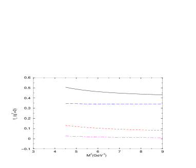
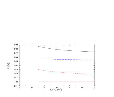
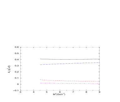
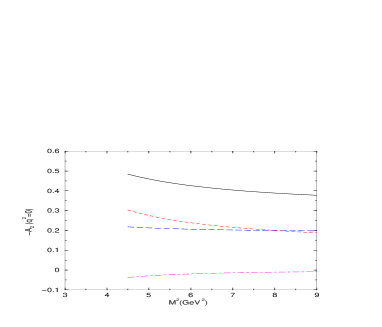
Figure 2: Various contributions to the OPE of the form factors as a function of the Borel parameter $M^{2}$. Solid curve: total contribution; long-dashed: perturbative; dashed: quark condensate; dot-dashed mixed condensate contribution.

$$0.40\leq f_{+}(0)\leq 0.48,\;\;\;\;\;\;\;\; 0.71\leq V(0)\leq 0.89\;,$$

$$0.32\leq A_{1}(0)\leq 0.42,\;\;\;\;\;\;\; - 0.43\leq A_{2}(0)\leq-0.37.$$ (36)

The value obtained for $f_{+}(0)$ is smaller than the value obtained for the same form factor in ref. detc by using the constituent quark meson model.

The $t$ dependence of the form factors evaluated at $M^{2}=7\nobreak\,\mbox{GeV}^{2}$ is shown in Fig. 3. In the range $-0.5\leq t\leq 0.4\;\nobreak\,\mbox{GeV}^{2}$ no non-Landau singularities occur for our choices of the continuum thresholds. The QCD sum rules results can, in this $t$-range, be very well approximated by a monopole expression

$$F(t)={F(0)\over 1-{t\over M_{P}^{2}}}\;,$$ (37)

for all four form factors. The reult of the fit is also shown in Fig. 3. the different values for the pole mass, $M_{P}$, for the different form factors are given by:

$$\begin{array}[]{c}M_{P}=\end{array}\left\{\begin{array}[]{c}(1.6\pm 0.2)\nobreak\,\mbox{GeV}\mbox{ for }f_{+}(t)\\ (4.2\pm 0.5)\nobreak\,\mbox{GeV}\mbox{ for }A_{1}(t)\\ (8.0\pm 2.0)\nobreak\,\mbox{GeV}\mbox{ for }A_{2}(t)\\ (1.95\pm 0.10)\nobreak\,\mbox{GeV}\mbox{ for }V(t)\end{array}\right.$$ (38)

In the case of $A_{2}$ we get a very hight $M_{P}$ showing a very weak $t$ dependence. This approximate $t$ independence stems from a mutual cancelation in the sum rule of an increase in the perturbative and a decrease in the quark condensate contributions. Even for $A_{1}$ the $t$ dependence is much weaker than for $f_{+}$ and $V$. It is also interesting to notice that $M_{P}^{(V)}$ is of the same order than the one for the semileptonic $D\rightarrow K^{*}\ell\nu_{\ell}$ found in bbd91 , and $M_{P}^{(f_{+})}$ is compatible with the ones found for the $D_{s}$ decays into $\eta$ cofa and $D\to\kappa\ell\nu_{\ell}$ dfnn .

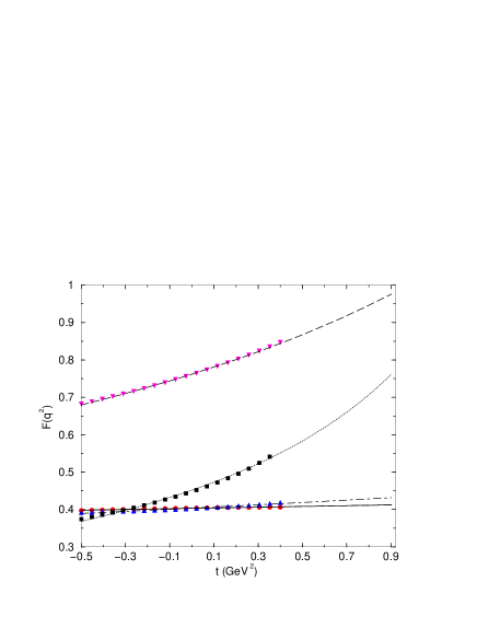
Figure 3: $t$ dependence of the form factors. The solid, dot-dashed, dotted and dashed lines give the monopole parametrization, in Eq.(37), to the QCD sum rule results for $-A_{2}$ (circles), $A_{1}$ (triangles up), $f_{+}$ (squares) and $V$ (triangles dow) respectively.

Having the form factors we can evaluate the decay widths for the $D_{s}^{+}\rightarrow\phi\pi^{+}$ and $D_{s}^{+}\rightarrow\phi\ell^{+}\nu_{\ell}$ decays, given by Eqs. (4) and (15) respectively. We obtain the following branching ratios:

$${\cal B}(D_{s}^{+}\to\phi\pi^{+})=(2.8\pm 0.7)\%\;,$$ (39)

and

$${\cal B}(D_{s}^{+}\to\phi\ell^{+}\nu)=(1.4\pm 0.4)\%\;$$ (40)

where we have used $V_{ud}=V_{cs}=0.975$, $f_{\pi}=0.132$ and the values $c_{1}(m_{c})=1.263$ and $c_{2}(m_{c})=-0.513$, corresponding to the results for the Wilson coefficients obtained at the leading order in renormalization group improved perturbation theory at $\mu\simeq 1.3\nobreak\,\mbox{GeV}$ cofa . The errors in the above results were estimated only by taking into account the uncertainties in the form factors in Eq. (36) and should be understood as limiting values for the branching ratios.

We see that, within the errors, our results are compatible with the experimental results given in Eqs. (2) and (3). Therefore, in the case of the $D_{s}$ decay into $\phi$, we can say that the factorization approximation works well. From this it seems reasonable to suppose that, if $f_{0}(980)$ has a dominant $\bar{s}s$ component, the factorization approximation should also work well for the $D_{s}$ decay into $f_{0}(980)$. Using Eqs. (4), (5) and (7), and the values for the form factors at $t=0$ given in Eq.(36) we get:

$${\Gamma(D_{s}^{+}\rightarrow f_{0}(980)\pi^{+})\over\Gamma(D_{s}^{+}\rightarrow\phi\pi^{+})}=0.44\pm 0.18\;.$$ (41)

In the recently measured spectra from the reaction $D_{s}^{+}\to\pi^{+}\pi^{+}\pi^{-}$ Ait01 , the relative weight of the channel $\pi^{+}f_{0}(980)$ is evaluated to be

$${{\cal B}(D_{s}^{+}\to\pi^{+}f_{0}(980)){\cal B}(f_{0}(980)\to\pi^{+}\pi^{-})\over{\cal B}(D_{s}^{+}\to\pi^{+}\pi^{+}\pi^{-})}=(56.5\pm 6.4)\%\;,$$ (42)

and the ratio of yields

$${\Gamma(D_{s}^{+}\rightarrow\pi^{+}\pi^{+}\pi^{-})\over\Gamma(D_{s}^{+}\rightarrow\phi\pi^{+})}=0.245\pm 0.028^{+0.019}_{-0.012}\;,$$ (43)

is measured. Taking into account the results in Eqs. (42) and (43) one gets:

$$R={\Gamma(D_{s}^{+}\rightarrow f_{0}(980)\pi^{+})\over\Gamma(D_{s}^{+}\rightarrow\phi\pi^{+})}={0.140\pm 0.046\over{\cal B}(f_{0}\to\pi^{+}\pi^{-})}\;.$$ (44)

Using the branching ratio ${\cal B}(f_{0}(980)\to\pi^{+}\pi^{-})\simeq 53\%$, the authors in ref. adn have estimated the ratio $R$ to be $R=0.275(1\pm 0.25)$. In a different way E791, using couple-channel Breit-Wigner function Ait01 , found a non significative $g_{K}$, that means indirectly a non significative contribution for the decay channel $f_{0}(980)\to KK$. Thus if we assume that ${\cal B}(f_{0}(980)\to\pi\pi)\sim 1$ which implies ${\cal B}(f_{0}(980)\to\pi^{+}\pi^{-})\sim 2/3$ (2/3 being the isospin factor), using this in Eq. (44) we get

$${\Gamma(D_{s}^{+}\rightarrow f_{0}(980)\pi^{+})\over\Gamma(D_{s}^{+}\rightarrow\phi\pi^{+})}=0.210\pm 0.069\;.$$ (45)

Therefore, from our result in Eq. (41), we conclude that there is a significant deviation from the factorization approximation for the $D_{s}^{+}\rightarrow f_{0}(980)\pi^{+}$ decay. This could be an indication that there is a sizeable nonstrange component in the $f_{0}(980)$ meson, or even that the $f_{0}(980)$ structure is more complex than indicated by the naive quark model.

It is interesting to notice that the result obtained in ref. detc for the ratio in Eq. (1) is very similar to our result in Eq. (41). However, the authors in detc concluded that their result supports a description of $f_{0}(980)$ as a $s\bar{s}$ state with a possible virtual $K\bar{K}$ cloud, but with no substantial mixture of $u\bar{u},~{}d\bar{d}$. We believe that this conclusion was reached because the authors in ref. detc misinterpreted the experimental result Ait01 . In their words, the E791 collaboration measured $R=0.62$, with a very small error. Since from the Particle Data Group PDG we only know that ${\cal B}(f_{0}\to\pi\pi)$ is dominant without knowing the exact number, there is still an indetermination in the ratio Eq. (44). As explained above, if we consider ${\cal B}(f_{0}\to\pi^{+}\pi^{-})\sim 2/3$, we arrive at the result in Eq. (45), which is smaller than our result in Eq. (41), leading us to an opposite conclusion compared with detc .

One possible way to test if there really is a sizeable nonstrange component in the $f_{0}(980)$ is through the measurement of the semileptonic $D_{s}^{+}\to f_{0}(980)\ell^{+}\nu$ decay, since in this decay we do not have problems with the factorization approximation. Our predicition for the branching ratio obtained from Eq.(10), by supposing $f_{0}(980)$ as a $\bar{s}s$ state, is:

$${\cal B}(D_{s}^{+}\to f_{0}(980)\ell^{+}\nu)=(0.55\pm 0.10)\%\;.$$ (46)

Any significant deviation from that will definitively imply in a sizeable nonstrange component in the $f_{0}(980)$ meson, which could be or not accomodated in the naive quark model. Therefore, we urge the experimentalists to search for this decay.

V Summary and conclusions

We have presented a QCD sum rule study of the $D_{s}^{+}$ decays to final states containing $\phi$ and $f_{0}(980)$ mesons. We have evaluated the $t$ dependence of the form factors $f_{+}(t)$, $A_{1}(t)$, $A_{2}(t)$ and $V(t)$ in the region $-0.5\leq t\leq 0.4\nobreak\,\mbox{GeV}^{2}$. The $t$ dependence of the form factors could be fitted by a monopole form and extrapolated to the full kinematical region. The axial-vector form factors $A_{1}$ and $A_{2}$ have a much weaker $t$ dependence than the form factors $f_{+}$ and $V$.

The form factors were used to evaluate the branching ratios for the decays $D_{s}^{+}\to\phi\pi^{+}$ and $D_{s}^{+}\to\phi\ell^{+}\nu_{\ell}$ and we have obtained a good agreement with experimental data. Since the evaluation of the decay width, in the nonleptonic decay, is based on the factorization approximation, our first conclusion is that the factorization approximation works well in the case of the decay $D_{s}^{+}\to\phi\pi^{+}$.

We have also evaluated the ratio $D_{s}^{+}\to f_{0}(980)\pi^{+}/(D_{s}^{+}\to\phi\pi^{+})$ and we got a result bigger than estimate based on experimental data. Based on the fact that factorization approximation works well in the case of the decay $D_{s}^{+}\to\phi\pi^{+}$, this result can be interpretated as an indication that there is a sizeable nonstrange component in the $f_{0}(980)$ meson, or even that the $f_{0}(980)$ structure is more complex than indicated by the naive quark model. This hypothesis could be tested by the measurement of the semileptonic $D_{s}^{+}\to f_{0}(980)\ell^{+}\nu$ decay, since there is no problem with the factorization approximation in the semileptonic decays.

Acknowledgements: We would like to thank H.G. Dosch for giving us the idea for this calculation and F.S. Navarra for fruitful discussions. This work has been supported by CNPq and FAPESP (Brazil).

Appendix A Two-point sum rules

In ref. faz the two-point sum rule for the $f_{0}(980)$ meson was evaluated by considering $f_{0}$ as a $\bar{s}s$ state. They got:

$$m_{f_{0}}^{2}f_{f_{0}}^{2}e^{-m_{f_{0}}^{2}/M^{2}} = {3\over 8\pi^{2}}\int_{4m_{s}^{2}}^{u_{0}}duu\left(1-{4m_{s}^{2}\over u}\right)^{3/2}e^{-u/M^{2}}$$ (47)

$$+ m_{s}e^{-m_{s}^{2}/M^{2}}\left[\langle\bar{s}s\rangle\left(3+{m_{s}^{2}\over M^{2}}\right)+{\langle\bar{s}g_{s}\sigma.Gs\rangle\over M^{2}}\left(1-{m_{s}^{2}\over 2M^{2}}\right)\right]\;.$$

Considering $M^{2}$ in the interval $1\leq M^{2}\leq 2\nobreak\,\mbox{GeV}^{2}$, $u_{0}=1.6\pm 0.1\nobreak\,\mbox{GeV}^{2}$ they got

$$f_{f_{0}}=(0.180\pm 0.015)\nobreak\,\mbox{GeV}.$$ (48)

If we consider $m_{s}^{2}=0$, the result for $f_{f_{0}}$ does not change significantly, and we get $f_{f_{0}}=(0.19\pm 0.02)\nobreak\,\mbox{GeV}$.

The sum rule for $\phi$ is given by rr :

$$f_{\phi}^{2}e^{-m_{\phi}^{2}/M^{2}}={1\over 4\pi^{2}}\int_{4m_{s}^{2}}^{u_{0}}du{(u+2m_{s}^{2})\sqrt{u-4m_{s}^{2}}\over u^{3/2}}e^{-u/M^{2}}+{2m_{s}\langle\bar{s}s\rangle\over M^{2}}+{\langle g^{2}G^{2}\rangle\over 48\pi^{2}M^{2}}.$$ (49)

Considering $m_{s}$ at most linearly and using $u_{0}=2.0\pm 0.1\nobreak\,\mbox{GeV}^{2}$ we get

$$f_{\phi}=(0.232\pm 0.010)\nobreak\,\mbox{GeV},$$ (50)

in the interval $1\leq M^{2}\leq 2\nobreak\,\mbox{GeV}^{2}$, in a very good agreement with the experimental value $f_{\phi}^{exp}=0.234\nobreak\,\mbox{GeV}$ PDG .

For $f_{D_{s}}$ the two point sum rule is given by:

$${m_{D_{s}}^{4}f_{D_{s}}^{2}\over(m_{c}+m_{s})^{2}}e^{-m_{D_{s}}^{2}/M^{2}}={3\over 8\pi^{2}}\int_{(m_{c}+m_{s})^{2}}^{s_{0}}ds(1-{(m_{c}-m_{s})^{2}\over s}\bigg{)}\sqrt{\lambda(s,m_{c}^{2},m_{s}^{2})}e^{-s/M^{2}}$$ (51)

$$+ \langle\bar{s}s\rangle e^{-m_{c}^{2}/M^{2}}\left(-m_{c}+{m_{s}\over 2}+{m_{s}m_{c}^{2}\over M^{2}}\right)-{m_{c}\langle\bar{s}g_{s}\sigma.Gs\rangle\over 2M^{2}}e^{-m_{c}^{2}/M^{2}}\left(1-{m_{c}^{2}\over 2M^{2}}\right)\;.$$

Considering $m_{s}$ at most linearly and using $s_{0}=8.8\nobreak\,\mbox{GeV}^{2}$ we get

$$f_{D_{s}}=(0.22\pm 0.02)\nobreak\,\mbox{GeV},$$ (52)

in the interval $2.3\leq M^{2}\leq 4.5\nobreak\,\mbox{GeV}^{2}$, in a good agreement with the value quoted in ref. ck00 , and also with recent lattice determination lat : $f_{D_{s}}=(0.252\pm 0.009)\nobreak\,\mbox{GeV}$.

Appendix B Perturbative Contributions to the three-point functions

In all this work we take into account the mass of the strange quark at most linearly. We have checked that the contibution of terms proportional to $m_{s}^{2}$ and higher powers are negligible. The perturbative contributions for the sum rules defined in Sec. III are:

$$\rho_{+}(s,u,t) = {3\over\lambda^{3/2}(s,u,t)}\left\{u\left[2m_{c}m_{s}(2m_{c}^{2}-s-t+u)+m_{c}^{2}(s-t+u)+s(-s+t+u)\right]\right.$$ (53)

$$- \left.(2m_{c}^{2}-s-t+u)(su+m_{c}m_{s}(s-t+u))\right\}\theta(s-s_{M}),$$

$$\rho_{1}(s,u,t) = -{3\over 2\lambda^{3/2}(s,u,t)}\left\{m_{c}u\left[\lambda(s,u,t)+2m_{c}^{2}(m_{c}^{2}-s-t+u)+2st\right]\right.$$ (54)

$$+ m_{s}\left[s^{3}-t^{3}+2ut^{2}+ut(2m_{c}^{2}-u)-2m_{c}^{2}u(m_{c}^{2}+u)\right.$$

$$- \left.\left.s^{2}(3t+2u)+s(3t^{2}-2tu+u(2m_{c}^{2}+u))\right]\right\}\theta(s-s_{M}),$$

$$\rho_{2}(s,u,t) = {3\over 2\lambda^{5/2}(s,u,t)}\left\{m_{c}u(s-t-u)\left[\lambda(s,u,t)+6st+6m_{c}^{2}(m_{c}^{2}-s-t+u)\right]\right.$$ (55)

$$+ m_{s}\left[s^{4}+t^{4}-t^{3}u+2m_{c}^{2}u^{2}(3m_{c}^{2}+u)-ut^{2}(10m_{c}^{2}+u)\right.$$

$$- s^{3}(4t+3u)+tu(6m_{c}^{4}+8m_{c}^{2}u+u^{2})+s^{2}(6t^{2}-tu+u(2m_{c}^{2}+3u))$$

$$- \left.\left.s(4t^{3}-5t^{2}u-4tu(2m_{c}^{2}+u)+u(6m_{c}^{4}+4m_{c}^{2}u+u^{2}))\right]\right\}\theta(s-s_{M}),$$

$$\rho_{V}(s,u,t) = {3\over 2\lambda^{3/2}(s,u,t)}\left\{m_{c}u\left(2m_{c}^{2}-s-t+u\right)\right.$$ (56)

$$+ \left.m_{s}\left[s^{2}+t^{2}-ut-2um_{c}^{2}-s(2t+u)\right]\right\}\theta(s-s_{M}),$$

where

$$s_{M}=m_{c}^{2}+{m_{c}^{2}u\over m_{c}^{2}-t}.$$ (57)

References

(1) Particle Data Group, K.Hagiwara et al., Phys. Rev.D66, 010001 (2002).
(2) F.E. Close and N.A. Törnqvist, J. Phys.G28, R249 (2002).
(7) J. Weinstein and N. Isgur, Phys. Rev. Lett.48,
659 (1982); Phys. Rev.D41, 2236 (1997).
(8) N. Brown and F.E. Close, In The DANE Physics
Handbook, L. Maiani, G. Pancheri and N. Paver eds, INFN Frascati, 1995, pp.
447; F.E. Close, N. Isgur and S. Kumano, Nucl. Phys.B389, 513
(1993).
(9) F. de Fazio and M.R. Pennington, Phys. Lett.B521,
15 (2001).
(11) V.V. Anisovich, L.G. Dakhno and V.A. Nikonov,
hep-ph/0302137.
(12) A. Deandrea et al., Phys. Lett.B502,
79 (2001).
(13) P. Ball, V.M. Braun and H.G. Dosch, Phys. Rev.,
D44, 3567 (1991).
(14) G. Buchalla, A.J. Buras and M.E. Lautenbacher, Rev.
Mod. Phys.68,1125 (1996).
(15) M.A. Shifman, A.I. and Vainshtein and V.I. Zakharov,
Nucl. Phys., B147, 385 (1979).
(16) R.S. Marques de Carvalho et al., Phys. Rev.D60,
034009 (1999).
(17) P. Colangelo and F. de Fazio, Phys. Lett.B520,
78 (2001).
(18) H.G. Dosch, E.M. Ferreira, F.S. Navarra and M. Nielsen,
Phys. Rev., D65, 114002 (2002).
(19) L.J. Reinders and H.R. Rubinstein, Phys. Lett.B145,
108 (1984).
(20) P. Colangelo and A. Khodjamirian,
QCD sum rules: A modern perspective, in At the Frontier of
Particle Physics, ed. M. Shifman, Singapore 2001, hep-ph/0010175.
(21) Alpha Collaboration, A. Jütner and J. Rolf, hep-lat/0302016.