Abstract

The propagation of hard partons through spatially extended matter leads to medium-modifications of their fragmentation pattern. Here, we review the current status of calculations of the corresponding medium-induced gluon radiation, and how this radiation affects hadronic observables at collider energies.

Chapter 0 Gluon Radiation and Parton Energy Loss

Contents

1. 0 Gluon Radiation and Parton Energy Loss
   1. 1 Introduction
   2. 2 Gluon Bremsstrahlung in the Eikonal Approximation
      1. 1 N=1 opacity approximation (single hard scattering limit)
      2. 2 Multiple soft scattering limit (dipole approximation)
   3. 3 Gluon Radiation beyond the Eikonal Approximation
      1. 1 Wilson Lines for Non-Eikonal Trajectories
      2. 2 Target averages for non-eikonal Wilson lines
      3. 3 The medium-induced gluon radiation spectrum
   4. 4 Properties of the medium-induced gluon radiation spectrum
      1. 1 Multiple soft scattering
      2. 2 Opacity Expansion of the radiation cross section
   5. 5 Applications
      1. 1 Properties of Quenching Weights
      2. 2 Quenching factors for hadronic spectra
      3. 3 Medium-modified fragmentation functions
   6. 6 Appendix A: Eikonal calculations in the target light cone gauge.
   7. 7 Appendix B: Path integral formalism for the photon radiation spectrum

1 Introduction

In the QCD improved parton model, inclusive cross sections for high-$p_{\perp}$ partons (observed as leading hadrons or jets) can be calculated through collinear factorization. This formalism convolutes the perturbatively calculable parton-parton cross sections with non-perturbative but process-independent (“initial state”) parton distribution functions and (“final state”) fragmentation functions. What additional physics input is needed if one extends the application of QCD to the description of inclusive high-$p_{\perp}$ parton cross sections in nucleus-nucleus collisions at RHIC or LHC, where hadronic projectiles have significant spatial extension $\propto A^{1/3}$ ?

The current discussion of this question focuses in particular on the following effects: (i) The density of the incoming parton distributions increases for given $x$ and $Q^{2}$ by a factor $\approx A^{1/3}$. This implies that with increasing $A^{1/3}$ the non-linear modifications [21, 47, 11, 29, 35] of the QCD evolution equations become relevant at lower center of mass energies (or larger momentum fractions $x$). (ii) The QCD evolution of the projectile wave function may be altered due to the presence of a spatially extended “target” through which it propagates[13]. This goes under the name “initial state partonic energy loss”. It is discussed e.g. in Drell-Yan production in $p-A$ where a quark in the proton may undergo multiple scattering in the nucleus on its route to annihilation [14, 32]. (iii) The hard partonic collision is well-localized on a scale $1/Q$ which is much smaller than the diameter of a nucleon $1/\Lambda_{QCD}$. Thus, one does not expect medium-modifications of the hard partonic cross section itself. However, there is a class of high-$p_{\perp}$ observables in e-A and p-A for which the medium-modification can be described by nuclear enhanced twist-four matrix elements whose importance is determined by the pole structure of the hard partonic cross section [43, 44, 50]. This is the only case of a nuclear dependence for which higher twist factorization theorems are proven. iv) At sufficiently large center of mass energy or for sufficiently extended projectiles ($A^{1/3}>1$), the probability of two independent hard parton interactions in the same hadronic collision becomes significant [49]. This is e.g. a significant background to some of the hadronic Higgs decay channels searched for in p-p collisions at the LHC [16]. (v) Finally, the presence of spatially extended matter can affect the fragmentation and hadronization of hard partons produced in nucleus-nucleus collisions[12, 24, 3]. This effect is often referred to as “final state partonic energy loss” or “jet quenching” and is expected to affect essentially all high-$p_{\perp}$ hadronic observables in heavy ion collisions at collider energies. The main motivation for the study of these observables is that the degree of nuclear modification may allow for a detailed characterization of the hot and dense matter produced in the collision.

All the above mentioned effects should emerge from a theory of QCD processes in nuclear matter. The development of such a theory is still at the very beginning. The high rate at which new data are becoming available from RHIC, as well as the rapid development of new theoretical ideas and phenomenological interpretations make it likely that any comprehensive review will be outdated very soon. In this situation, we have decided to focus entirely on a simple partonic multiple scattering formalism which underlies at present almost all “jet quenching” calculations. This limited scope excludes many important issues. In particular, we do not discuss to what extent experimental data from RHIC provide indications of partonic energy loss (see [46]). Moreover, many phenomenologically proposals for discovering partonic energy loss, such as the measurement of back-to-back correlations[12, 54, 55], the specific behavior of massive $b$-quarks [18, 41, 42, 17] or particle ratios at high $p_{\perp}$ are not included in the discussion. Finally, we do not discuss recent alternative formulations of partonic energy loss, e.g. in the framework of nuclear enhanced higher twist matrix elements  [23, 56].

The presentation is organized as follows: in section 2, we discuss the formalism of eikonal scattering in which $S$-matrix amplitudes are determined in terms of eikonal Wilson lines in the target field. Section 3 discusses the generalization of this formalism to non-eikonal trajectories which take the transverse Brownian motion of the partonic projectile into account. The medium-induced gluon energy distribution radiated off a hard parton is calculated in this generalized formalism. Section 4 discusses the properties of this medium-induced spectrum and section 5 turns to some applications.

2 Gluon Bremsstrahlung in the Eikonal Approximation

At high energy, the propagation time of a parton through a target is short, partons propagate independently of each other and their transverse positions do not change during the propagation. The only effect of the propagation is that the wave function of each parton in the projectile acquires an eikonal phase due to the interaction with the target field[15, 38]. To be specific, we consider a hadronic projectile wave function whose relevant degrees of freedom are the transverse positions and color states of the partons,

$$\Psi_{in}=\sum_{\{\alpha_{i},{\bf x}_{i}\}}\,\psi(\{\alpha_{i},{\bf x}_{i}\})\,|\{\alpha_{i},{\bf x}_{i}\}\rangle\,.$$ (1)

The color index $\alpha_{i}$ can belong to the fundamental, anti fundamental or adjoint representation of the color $SU(N)$ group, corresponding to quark, anti quark or gluon in the wave function. We choose the Lorentz frame in which the projectile moves in the negative $z$ direction. Thus at high energy the light cone coordinate $x^{+}$ of the projectile does not change during the propagation thought the target. The projectile emerges form the interaction region with the wave function

$$\Psi_{out}={\cal S}\Psi_{in}=\sum_{\{\alpha_{i},{\bf x}_{i}\}}\psi(\{\alpha_{i},{\bf x}_{i}\})\prod_{i}W({\bf x}_{i})_{\alpha_{i}\beta_{i}}\,|\{\beta_{i},{\bf x}_{i}\}\rangle\,.$$ (2)

Here ${\cal S}$ is the $S$-matrix, and the $W$’s are Wilson lines along the (straight line) trajectories of the propagating particles

$$W({\bf x}_{i})={\cal P}\exp\{i\int dz^{-}T^{a}A^{+}_{a}({\bf x}_{i},z^{-})\}$$ (3)

with $A^{+}$ - the gauge field in the target and $T^{a}$ - the generator of $SU(N)$ in a representation corresponding to a given parton.

The interaction in the target field changes the relative phases between components of the wave function and thus “decoheres” the initial state. As a result the final state is different from the initial one, and contains emitted gluons.

The component of the outgoing wave function which belongs to the subspace orthogonal to the incoming state reads

$$|\delta\Psi\rangle = \left[1-|\Psi_{in}\rangle\langle\Psi_{in}|\right]|\Psi_{out}\rangle\,.$$ (4)

From this, one can calculate for example the inelastic cross section which up to the factor of total flux is given by the probability

$$P_{\rm inel}=|\delta\Psi|^{2}=1-|s|^{2}\,,$$ (5)

where

$$s=\langle\Psi_{in}|\Psi_{out}\rangle\,.$$ (6)

The $S$-matrix element in eq.(6) has to be averaged over the distribution of the color fields in the target. Also, the total and diffractive cross sections can be calculated by projecting other components out of $\Psi_{out}$ [38].

In what follows, we apply the above framework to calculate the gluon radiation spectrum radiated off a hard quark which propagates at high energy through a nuclear target. At this point we assume the quark to be coming from outside the target rather than being produced inside the target in a hard scattering event. Thus it carries with it the fully developed wave function which contains the cloud of quasi real gluons.

In the first order in perturbation theory the incoming wave function contains the Fock state $|\alpha\rangle$ of the bare quark, supplemented by the coherent state of quasi real gluons which build up the Weizsäcker-Williams field $f({\bf x})$,

$$\Psi_{\rm in}^{\alpha} = |\alpha\rangle+\int d{\bf x}\,d\xi f({\bf x})\,T^{b}_{\alpha\,\beta}\,|\beta\,;b({\bf x},\xi)\rangle$$

Here Lorentz and spin indices are suppressed. In the projectile light cone gauge $A^{-}=0$, the gluon field of the projectile is the Weizsäcker-Williams field

$$A^{i}({\bf x})\propto\theta(x^{-})\,f_{i}({\bf x})\,,\qquad\qquad f_{i}({\bf x})\propto g{{\bf x}_{i}\over{\bf x}^{2}}\,,$$ (8)

where $x^{-}=0$ is the light cone coordinate of the quark in the wave function. The integration over the rapidity of the gluon in the wave function (2) goes over the gluon rapidities smaller than that of the quark. In the leading logarithmic order the wave function does not depend on rapidity and we suppress the rapidity label in the following.

The interaction of the projectile (2) with the target leads to a color rotation $\alpha_{i}\to\beta_{i}$ of each projectile component $i$, resulting in an eikonal phase $W({\bf x}_{i})_{\alpha_{i}\beta_{i}}$. The outgoing wave function reads

$$\Psi_{\rm out}^{\alpha} = W^{F}_{\alpha\,\gamma}({\bf 0})\,|\gamma\rangle+\int d{\bf x}\,f({\bf x})\,T_{\alpha\,\beta}^{b}W_{\beta\,\gamma}^{F}({\bf 0})\,W_{b\,c}^{A}({\bf x})\,|\gamma\,;c({\bf x})\rangle\,,$$ (9)

where $W^{F}({\bf 0})$ and $W^{A}({\bf x})$ are the Wilson lines in the fundamental and adjoint representations respectively, corresponding to the propagating quark at the transverse position ${\bf x}_{q}={\bf 0}$ and gluon at ${\bf x}_{g}={\bf x}$. Gluon radiation is an inelastic process, for which we have to calculate the projection (4)

$$|\delta\Psi_{\alpha}\rangle=|\Psi_{\rm out}^{\alpha}\rangle-\sum_{\gamma}|\Psi_{\rm in}(\gamma)\rangle\langle\Psi_{in}(\gamma)|\Psi_{out}^{\alpha}\rangle$$ (10)

Here, the index $\gamma$ in the projection operator runs over the quark color index. It appears in eq.(10) since we have to project out the components of the wave function which differ from the initial state only by a global rotation in the color space [38].

The number spectrum of produced gluons is obtained from (10) by calculating the expectation value of the number operator in the state $\delta\Psi_{\alpha}$, averaged over the incoming color index $\alpha$. After some color algebra, one obtains

$$N_{\rm prod}({\bf k})=\frac{1}{N}\sum_{\alpha}\langle\delta\Psi_{\alpha}|a_{d}^{\dagger}({\bf k})\,a_{d}({\bf k})|\,\delta\Psi_{\alpha}\rangle$$

$$\quad=\frac{\alpha_{s}\,C_{F}}{2\pi}\,\int d{\bf x}\,d{\bf y}\,e^{i{\bf k}\cdot({\bf x}-{\bf y})}\frac{{\bf x}\cdot{\bf y}}{{\bf x}^{2}\,{\bf y}^{2}}\Bigg{[}1-\frac{1}{N^{2}-1}\,\langle\langle{\rm Tr}\left[W^{A\,\dagger}({\bf x})\,W^{A}({\bf 0})\right]\rangle\rangle_{t}$$

$$\qquad\qquad\qquad\qquad\qquad\qquad-\frac{1}{N^{2}-1}\,\langle\langle{\rm Tr}\left[W^{A\,\dagger}({\bf y})\,W^{A}({\bf 0})\right]\rangle\rangle_{t}$$

$$\qquad\qquad\qquad\qquad\qquad\qquad+\frac{1}{N^{2}-1}\,\langle\langle{\rm Tr}\left[W^{A\,\dagger}({\bf y})\,W^{A}({\bf x})\right]\rangle\rangle_{t}\Bigg{]}\,.$$ (11)

Here, we have used $f({\bf x})\,f({\bf y})=\frac{\alpha_{s}}{2\pi}\,\frac{{\bf x}\cdot{\bf y}}{{\bf x}^{2}\,{\bf y}^{2}}$ for the Weizsäcker-Williams field of the quark projectile in configuration space and the symbol $\langle\rangle_{t}$ denotes the averaging over the gluon fields of the target.

To obtain an explicit expression, we require the target average of the product of adjoint Wilson lines. Various averaging procedures are discussed in the literature [61, 15, 57, 58, 38]. To be specific, we consider a target which consists of static scattering centers with scattering potentials $a_{a}^{+}({\bf q})$ at positions $(\hat{\bf x}_{n},\hat{z}_{n})$. In the high energy approximation, each scattering center transfers only transverse momentum to the projectile,

$$A_{a}^{+}({\bf x},z^{-})=\sum_{n}\int\frac{d^{2}{\bf q}}{(2\pi)^{2}}e^{i({\bf x}-\hat{\bf x}_{n})\cdot{\bf q}}\,a_{a}^{+}({\bf q})\,\delta(z^{-}-\hat{z}^{-}_{n})\,.$$ (12)

We define the target average as an average over the transverse positions of the static scattering centers. Introducing the longitudinal density of scattering centers, $n(z^{-})=\sum_{n}\delta(z^{-}-\hat{z}^{-}_{n})$, we find

$$\langle\langle\int dz^{-}\,d\tilde{z}^{-}\,A_{a}^{+}({\bf x},z^{-})\,A_{a}^{+}({\bf y},\tilde{z}^{-})\rangle\rangle_{t}=\int d\xi\,n(\xi)\,\frac{C_{A}}{2}\,\sigma({\bf x}-{\bf y})\,,$$ (13)

where we have defined the dipole cross section

$$\sigma({\bf x}-{\bf y})=2\int\frac{d^{2}{\bf q}}{(2\pi)^{2}}|a^{+}({\bf q})|^{2}\,\left(1-e^{i{\bf q}\cdot({\bf x}-{\bf y})}\right)\,.$$ (14)

We now consider the gluon number spectrum (11) in two limiting cases.

1 N=1 opacity approximation (single hard scattering limit)

This limit is relevant for a small target with weak target fields $A^{+}=O(g)$. In this case the projectile can scatter at most once. Thus the adjoint Wilson lines can be expanded to leading order in the single scattering potential $a_{a}^{+}({\bf q})$. Using (13), we find

$$\frac{1}{N^{2}-1}\langle\langle{\rm Tr}\left[W^{A\,\dagger}({\bf x})\,W^{A}({\bf y})\right]\rangle\rangle_{t}\approx 1-\frac{1}{4\,C_{F}}\int d\xi\,n(\xi)\,\sigma({\bf x}-{\bf y})\,.$$ (15)

The corresponding gluon number spectrum reads

$$N_{\rm prod}({\bf k}) = \frac{\alpha_{s}C_{A}}{8\pi}\,\int d\xi\,n(\xi)\,d{\bf x}\,d{\bf y}\,e^{i{\bf k}\cdot({\bf x}-{\bf y})}\frac{{\bf x}\cdot{\bf y}}{{\bf x}^{2}\,{\bf y}^{2}}\Bigg{[}\sigma({\bf x})+\sigma({\bf y})-\sigma({\bf x}-{\bf y})\Bigg{]}$$ (16)

$$= \alpha_{s}\,\pi C_{A}\int d\xi\,n(\xi)\,\int\frac{d^{2}{\bf q}}{(2\pi)^{2}}|a^{+}({\bf q})|^{2}\,\frac{{\bf q}^{2}}{{\bf k}^{2}\,({\bf k}-{\bf q})^{2}}\,.$$

Differentiated with respect to the momentum transfer ${\bf q}$, this result is the well-known Gunion-Bertsch radiation cross section[22] for the gluon radiation cross section in quark-quark scattering,

$$\qquad\qquad=\frac{d\sigma^{\rm GB}}{d\ln x\,d{\bf q}\,d{\bf k}}=\frac{C_{A}\,\alpha_{s}}{\pi^{2}}|a^{+}_{\rm QCD}({\bf q})|^{2}\,\frac{{\bf q}^{2}}{{\bf k}^{2}\,({\bf k}-{\bf q})^{2}}\,.$$ (17)

Integrated over the transverse momentum exchanged with the “target” quark, this radiation spectrum can be written in terms of the dipole cross section (14),

$$\frac{d\sigma^{\rm GB}}{d\ln x\,d{\bf k}} = 4\,C_{A}\,\alpha_{s}\int\frac{d{\bf q}}{(2\,\pi)^{2}}\,\frac{{\bf q}^{2}}{{\bf k}^{2}\,({\bf k}-{\bf q})^{2}}\,$$ (18)

$$\qquad\qquad\times{-1\over 2}\int{d{\bf r}\over(2\pi)^{2}}\,\sigma_{\rm QCD}({\bf r})\,\exp\left\{i\,{\bf q}\cdot{\bf r}\right\}\,.$$

For a scattering on a static source described by a Yukawa type potential, one has $|a^{+}_{\rm QCD}({\bf q})|^{2}\propto\frac{\alpha_{\rm s}M^{2}}{\left(M^{2}+{\bf q}^{2}\right)^{2}}$. Although perturbatively gluons are massless, the screening mass $M$ is frequently introduced to mimic the medium effects which cut off the infrared divergence[24]. The factor $\alpha_{s}$ in this expression accounts for the fact that the gluon field in eqs.(13,14) is emitted by the single particle source. It is the presence of this coupling constant that justifies the expansion of the Wilson lines to leading order in $\sigma$.

It is interesting to compare the expression eq.(17) with the high energy limit of the Bethe-Heitler photon radiation cross section in QED,

$$\frac{d\sigma^{\rm BH}}{d\ln x\,d{\bf q}\,d{\bf k}}=\frac{\alpha_{\rm em}}{\pi^{2}}\,|a^{+}_{\rm QED}({\bf q})|^{2}\,\frac{x^{2}\,{\bf q}^{2}}{{\bf k}^{2}\,({\bf k}-x{\bf q})^{2}}$$ (19)

Here, ${\bf k}$ is the transverse photon momentum and $x=\omega_{\gamma}/E$ the fraction of the energy carried away by the photon. Again, if integrated over the transverse momentum transfer ${\bf q}$ from the target, this radiation spectrum can be written in terms of a dipole cross section

$$\frac{d\sigma^{\rm BH}}{d\ln x\,d{\bf k}} =-2\,\alpha_{\rm em}\int\frac{d{\bf q}\,d{\bf r}}{(2\,\pi)^{4}}\,\frac{{\bf q}^{2}}{{\bf k}^{2}\,({\bf k}-{\bf q})^{2}}\,\sigma_{\rm QED}(x\,{\bf r})\,e^{i\,{\bf q}\cdot{\bf r}}\,.$$ (20)

The radiation cross section (17) and (19) for QCD and QED differ only by their $x$-dependence. The QCD radiation is flat in rapidity, whereas the QED radiation cross section peaks at projectile rapidity $x=1$. The physical reason is that in QCD, the radiated gluon is charged. The distribution of gluons in the incoming quark wave function is flat in rapidity. Thus when a gluon scatters directly off a scattering center into the final state, the rapidity plateau is produced. It is the non-abelian diagram contributing to (17) which dominates the QCD radiation spectrum. This is also the reason why the explicit Casimir factor in (17) is the adjoint and not the fundamental one. In QED on the other hand only the electron can scatter directly off a source. This scattering is most effective for electrons with small fraction of longitudinal momentum. Such scattering events result in final state photons which carry most of the initial longitudinal momentum, and thus the photon spectrum is peaked around $x=1$.

In configuration space, the different $x$-dependence of the QCD and QED radiation spectrum is reflected in the different arguments of the dipole cross sections: the QCD dipole cross section is tested at transverse distances ${\bf r}$ but the QED one is tested at $x{\bf r}$. For an intuitive understanding of this behavior, consider the incoming projectile electron or quark in the light cone frame as a superposition of the bare particle and its higher Fock states,

$$|{\rm projectile}\rangle=|q\rangle+|q\,g\rangle+\dots\,.$$ (21)

If all Fock components interact with the scattering potentials with the same amplitude, then the coherence between these amplitudes is not disturbed, and no bremsstrahlung is generated. The radiation amplitude depends on the decoherence between the different Fock state elements, i.e., on the difference between the elastic scattering amplitudes of different fluctuations. This difference is characterized by the impact parameter difference between different Fock state components. It can be estimated from the transverse separation of the $|q\rangle$ and $|q\,\gamma\rangle$ fluctuations. On a characteristic time scale ${1\over\Delta E}=\left(\frac{k_{\perp}^{2}}{2x(1-x)E}\right)^{-1}$ set by the transverse energy of the two-particle Fock state, the quark, gluon or photon move in the impact parameter plane by distances

$$x_{\perp\,\gamma}\,,\,x_{\perp\,g} \propto {k_{\perp}\over x\,E}{1\over\Delta E}\propto{(1-x)\over k_{\perp}}\,,$$ (22)

$$x_{\perp\,q}\,,\,x_{\perp\,e} \propto {k_{\perp}\over(1-x)\,E}{1\over\Delta E}\propto{x\over k_{\perp}}\,.$$ (23)

Since the photon does not carry charge, the transverse distance $x_{\perp\,\gamma}$ plays no role in the decoherence of QED Fock state components, while the distance $x_{\perp\,g}$ plays the dominant role in the corresponding QCD process. The QED and QCD dipole cross sections thus measure the transverse separations

To leading order $O(1/x)$, the cross sections in (18) and (20) thus differ by a factor $x$ in the argument of $\sigma({\bf r})$. Based on the above picture, Nikolaev and Zakharov proposed[48] to write the dipole cross section for the $q\bar{q}g$- configuration beyond leading $O(1/x)$ as

$$\sigma_{\rm QCD}({\bf r},x) = {9\over 8}\,\left\{\bar{\sigma}({\bf r})+\bar{\sigma}((1-x)\,{\bf r})\right\}-{1\over 8}\,\bar{\sigma}(x\,{\bf r})\,,$$ (24)

where the prefactors account for the color representations of quark and gluon.

Due to this distinct $x$-dependence the QED expression cannot be obtained in the eikonal approximation. The eikonal limit where the energy loss of the electron is neglected is equivalent to the limit $x=0$, where according to eq.(19) no photons are emitted. In our wave function formalism this arises since the components of the wave function with no photons and with one photon rotate with the same phase during the propagation through the target, if the energies of the electron in both components are assumed to be the same. Thus in QED the eikonal approximation leads to the vanishing inelastic cross section. In QCD this is of course not the case, since the gluon component of the wave function scatters most efficiently.

2 Multiple soft scattering limit (dipole approximation)

We now consider the opposite limit, when the projectile undergoes many scatterings. Assume that these scatterings are independent in the sense that the vector potentials of the different scattering centers in eq.(12) are uncorrelated in color space. Then the dipole cross section in eq.(15) exponentiates. We also assume that the cross section is dominated by the low momentum transfer in each individual scattering. In this limit the dipole cross section $\sigma({\bf x}-{\bf y})$ can be approximated by the lowest order term in the Taylor expansion $\sigma({\bf x}-{\bf y})\propto({\bf x}-{\bf y})^{2}$. This is the so-called logarithmic approximation, in which the target correlator of two Wilson lines is characterized in terms of the saturation momentum $Q_{s}$,

$$\frac{1}{N^{2}-1}\,\langle\langle{\rm Tr}\left[W^{A\,\dagger}({\bf y})\,W^{A}({\bf x})\right]\rangle\rangle_{t} \approx \exp\left[-\frac{C_{A}}{4\,C_{F}}\int d\xi\,n(\xi)\,\sigma({\bf x}-{\bf y})\right]$$ (25)

$$\approx \exp\left[-{({\bf x}-{\bf y})^{2}\over 8}{C_{A}\over C_{F}}Q^{2}_{s}\right]\,.$$

Here, the saturation momentum is

$$Q_{s}^{2}=\int d\xi\,n(\xi)\,\int\frac{d{\bf q}}{(2\pi)^{2}}|a_{a}^{+}({\bf q})|^{2}\,{\bf q}^{2}\,,$$ (26)

which in the model (12) of the target fields characterizes the average transverse momentum squared transferred from the target to the projectile. Using the average (25) to calculate the produced gluon number spectrum (11), we obtain [34]

$$N_{\rm prod}({\bf k}) = \frac{\alpha_{s}\,C_{F}}{2\pi}\int d{\bf x}\,d{\bf y}\,e^{ik(x-y)}\,\frac{{\bf x}\cdot{\bf y}}{{\bf x}^{2}\,{\bf y}^{2}}$$ (27)

$$\times\left(1+e^{-({\bf x}-{\bf y})^{2}\,{C_{A}\over 8C_{F}}Q_{s}^{2}}-e^{-{\bf x}^{2}\,{C_{A}\over 8C_{F}}Q_{s}^{2}}-e^{-{\bf y}^{2}\,{C_{A}\over 8C_{F}}Q_{s}^{2}}\right)$$

$$= \frac{\alpha_{s}\,C_{F}}{(2\pi)^{3}}\frac{2\,C_{F}}{C_{A}\,Q_{s}^{2}}\frac{1}{\pi}\,\int d{\bf q}\,e^{-{2C_{F}\over C_{A}Q_{s}^{2}}{\bf q}^{2}}\,\frac{{\bf q}^{2}}{{\bf k}^{2}\,({\bf k}-{\bf q})^{2}}\,.$$

Expression (27) contains again the Gunion-Bertsch radiation cross section (17). In the dipole approximation (25), however, the entire medium acts coherently as a single scattering center with a Gaussian momentum distribution

$$|a_{+}({\bf q})|^{2}\propto e^{-{2C_{F}\over C_{A}Q_{s}^{2}}{\bf q}^{2}}\,.$$ (28)

There is an interesting attempt to generalize (27) to the case of a dense projectile realized in nucleus-nucleus collisions [36].

The eikonal approximation described in this section is valid as long as the average momentum transfer from the medium is much smaller than the longitudinal momentum of the produced gluon. Only in this limit all scattering centers contribute coherently to the production amplitude. The purpose of the following is to generalize (27) to the kinematic region where this is not necessarily the case, and incoherent scatterings also play an important role.

3 Gluon Radiation beyond the Eikonal Approximation

In the eikonal approximation, the Wilson lines (3) determine the $S$-matrix for the scattering of partonic wave functions. In this section, we derive the leading finite energy corrections $O(1/p^{-})$ to this high energy limit. We explain the form of the target averages including $O(1/p^{-})$ corrections and we give two applications: the photo absorption cross section and the medium-induced gluon radiation spectrum.

1 Wilson Lines for Non-Eikonal Trajectories

We consider the $N$-fold scattering amplitude of a high energy quark. In the light cone gauge $A^{-}=0$, it reads

$$F(x_{0},p) =$$ (29)

$$=\sum_{N=0}^{\infty}\prod_{i=1}^{N}{\cal P}\,\left(\int\frac{dp_{i}^{+}\,dp_{i}^{-}\,d{\bf p}_{i}}{(2\pi)^{4}}\int dx_{i}^{+}\,dx_{i}^{-}\,d{\bf x}_{i}\,\frac{i}{\not p_{i}-m+i\epsilon}\,\right.$$

$$\times\left.\left(-i\gamma^{-}\,A^{+}({\bf x}_{i},x_{i}^{-})\right)\,e^{ix_{i}^{+}\cdot(p^{-}_{i+1}-p^{-}_{i})+ix^{-}_{i}\cdot(p^{+}_{i+1}-p^{+}_{i})}e^{i{\bf x}_{i}\cdot({\bf p}_{i+1}-{\bf p}_{i})}\right)\,$$

$$\times e^{ix_{0}\cdot p_{1}}\,v(p)\,.$$

Here, the target gauge fields $A^{+}=A^{+}_{a}T_{a}$ are path-ordered along the trajectory of the quark; we suppress color and spin indices on the quark propagators and the spinor $v(p)$. The additional phase factor $e^{ix_{0}\cdot p_{1}}$ in (29) is useful in order to connect the multiple scattering diagram to the vertex of a more complicated amplitude by integration over $x_{0}$. In the absence of scattering centers, (29) reduces to a free quark wave function $e^{ix_{0}\cdot p}\,v(p)$.

We approximate eq. (29) to leading order $O\left(\left(1/p^{-}\right)^{0}\right)$ in the norm and to subleading order $O\left(1/p^{-}\right)$ in the phase. To this order we can neglect the dependence of the target fields on $x_{i}^{+}$, as indicated in (29). This is because the incoming quark propagates in the negative $z$ direction and thus only feels the fields at $x^{+}=0$. The integration over $x_{i}^{+}$ and $p_{i}^{-}$ is then trivial: all propagators have the same component $p_{i}^{-}=p^{-}$. To simplify (29) further, we use

$$\frac{1}{\not p-m}=\frac{\sum_{s}u_{s}(p)\,\bar{u}_{s}(p)}{p^{2}-m^{2}}+\frac{\gamma^{-}}{2p^{-}}\,,$$ (30)

and neglect the last term to leading order in the energy $1/p^{-}$. The spinor structure can be simplified:

$$\bar{u}_{s}(p)\left(-i\gamma\cdot A\right)u_{s^{\prime}}(p)\simeq p^{-}\,A^{+}\,\delta_{ss^{\prime}}\,.$$ (31)

With these simplifications, eq. (29) takes the form

$$F(x_{0},p) = \sum_{N=0}^{\infty}\prod_{i=1}^{N}{\cal P}\,\left(\int\frac{dp_{i}^{+}\,d{\bf p}_{i}}{(2\pi)^{3}}\int dx_{i}^{-}\,d{\bf x}_{i}\,\frac{-i}{p^{+}_{i}-({\bf p}_{i}^{2}+m^{2})/p^{-}+i\epsilon}\,\right.$$ (32)

$$\times\left.\left(iA^{+}({\bf x}_{i},x_{i}^{-})\right)\,e^{ip_{i}^{+}\cdot(x^{-}_{i-1}-x^{-}_{i})}e^{-i{\bf p}_{i}\cdot({\bf x}_{i-1}-{\bf x}_{i})}\right)\,$$

$$\times e^{ix^{+}_{0}\cdot p^{-}}e^{ix_{N}^{-}p^{+}-i{\bf x}_{N}\cdot{\bf p}}\,v(p)\,.$$

The spatial ordering of the scattering centers along the trajectory is fixed explicitly by performing the $p^{+}_{i}$-integrations. Neglecting the mass term, we find a product of $\Theta$-functions times phase factors

$$\int\frac{dp_{i}^{+}}{2\pi}\,\frac{i}{p^{+}_{i}-({\bf p}_{i}^{2}+m^{2})/p^{-}+i\epsilon}\,e^{ip_{i}^{+}(x^{-}_{i-1}-x^{-}_{i})}$$

$$\quad=e^{i\frac{{{\bf p}_{i}}^{2}}{p_{i}^{-}}\,(x^{-}_{i-1}-x^{-}_{i})}\,\Theta(x^{-}_{i}-x^{-}_{i-1})\,.$$ (33)

Inserting this expression into (32) and performing the transverse ${\bf p}_{i}$-integration, we obtain the basic building block of the formalism, the free light-cone Green’s function

$$G_{0}({\bf x}_{i-1},x^{-}_{i-1};{\bf x}_{i},x^{-}_{i}|p^{-})=\int\frac{d{\bf p}_{i}}{(2\pi)^{2}}e^{i\frac{{\bf p}_{i}^{2}}{p_{i}^{-}}\,(x^{-}_{i-1}-x^{-}_{i})}\,e^{-i{\bf p}_{i}\cdot({\bf x}_{i-1}-{\bf x}_{i})}$$

$$=\frac{p^{-}}{4\pi i(x^{-}_{i}-x^{-}_{i-1})}\,\exp\left[{\frac{ip^{-}({\bf x}_{i}-{\bf x}_{i-1})^{2}}{4\,(x^{-}_{i}-x^{-}_{i-1})}}\right]$$

$$=\int{\cal D}{\bf r}(\xi)\,\exp\left[\frac{ip^{-}}{4}\int_{x^{-}_{i-1}}^{x^{-}_{i}}d\xi\,\dot{\bf r}^{2}(\xi)\right]\,.$$ (34)

Here, $\dot{\bf r}=d{\bf r}/dz^{-}$ and the boundary conditions on the free path integral are ${\bf r}(x^{-}_{i})={\bf x}_{i}$. The limit $x_{i}^{-}-x_{i-1}^{-}\to 0$ of (34) is equivalent to the high- energy limit

$$\lim_{p^{-}\to\infty}G_{0}({\bf x}_{i-1},x^{-}_{i-1};{\bf x}_{i},x^{-}_{i}|p^{-})=\delta^{2}({\bf x}_{i-1}-{\bf x}_{i})\,.$$ (35)

The free Green’s function (34) evolves the free plane wave $e^{ix_{i}^{-}p^{+}-i{\bf x}_{i}\cdot{\bf p}}$ to the position $({\bf x}_{i-1},x^{-}_{i-1})$. The sum of the $N$-fold scattering amplitudes (29) reads

$$F(x_{0},p) = e^{ix^{+}_{0}\cdot p^{-}}\sum_{N=0}^{\infty}{\cal P}\,\Bigg{(}\prod_{i=1}^{N}\int dx_{i}^{-}\,d{\bf x}_{i}\,G_{0}({\bf x}_{i-1},x^{-}_{i-1};{\bf x}_{i},x^{-}_{i}|p^{-})$$ (36)

$$\qquad\times\Theta(x_{i}^{-}-x_{i-1}^{-})\,\left(iA^{+}({\bf x}_{i},x_{i}^{-})\right)\,\Bigg{)}\,e^{ix_{N}^{-}p^{+}-i{\bf x}_{N}\cdot{\bf p}}\,v(p)$$

$$= e^{ix^{+}_{0}\cdot p^{-}}\int d{\bf x}G({\bf x}_{0},x_{0}^{-};{\bf x},x^{-}|p^{-})\,e^{i\frac{{{\bf p}_{i}}^{2}}{p_{i}^{-}}\,x^{-}\,-i{\bf p}_{i}\cdot{\bf x}}v(p)\,,$$

where the full Green’s function is

$$G({\bf x}_{0},x_{0}^{-};{\bf x},x^{-}|p^{-})$$

$$\quad=\int{\cal D}{\bf r}(\xi)\,\exp\left[\frac{ip^{-}}{4}\int_{x^{-}_{i-1}}^{x^{-}_{i}}d\xi\,\dot{\bf r}^{2}(\xi)\right]\,W([{\bf r}];x_{0}^{-},x^{-})\,,$$ (37)

$$W([{\bf r}];x_{0}^{-},x^{-})={\cal P}\,\exp\left[i\int_{x_{0}^{-}}^{x^{-}}d\xi\,A^{+}({\bf r}(\xi),\xi)\right]\,.$$ (38)

These expressions give the leading $O(1/p^{-})$ corrections to the phase of the eikonal Wilson line (3). The path integral in (37) has a very simple interpretation. It describes the quantum mechanical particle which, while propagating through the medium can move in the transverse plane. The free transverse motion is governed by the kinetic term $\frac{p^{-}}{4}\dot{\bf r}^{2}$ - a two-dimensional light-cone hamiltonian with “mass” given by the total energy $p^{-}/2$ of the projectile along the beam. During the motion the wave function of the particle also acquires a phase given by the Wilson line along the trajectory. The infinite energy limit corresponds to the classical limit, where a single straight classical trajectory dominates the sum over paths. In this limit the Green’s function (37) reduces to the eikonal Wilson line in (3),

$$\lim_{p^{-}\to\infty}G({\bf x}_{0},x_{0}^{-};{\bf r},x^{-}|p^{-})=W({\bf r};x_{0}^{-},x^{-})\,\delta^{2}({\bf x}_{0}-{\bf r})\,.$$ (39)

Non-abelian Furry approximation (target field $A_{0}$)

The multiple scattering diagram (36) contains the leading order $O(1/p^{-})$ corrections to the phase of the eikonal Wilson line, but the norm of (36) is given to $O\left((1/p^{-})^{0}\right)$ only. For a scalar quark that would be the only important correction. For a spinor quark however this is not enough if one wants for example to discuss emission of on shell gluons. It turns out that the leading order of this propagator vanishes when connected to an emission vertex of a real gluon. To get a leading order result for this process one has to keep order $O(1/p^{-})$ corrections to the first propagator $1/(\gamma\cdot p_{1}-m)$. We now discuss the non Abelian Furry approximation which addresses this issue.

We also change our notations slightly in accordance with literature. The target field will not be described by a large $A^{+}$-component but rather specified by the Gyulassy-Wang model [24, 53] as a collection of scattering potentials of Yukawa-type with Debye screening mass $M$,

$$A_{\mu}({\bf x}) = \delta_{0\mu}\,\sum_{i=1}^{\infty}\,\varphi^{a}_{i}({\bf x})\,T^{a}\,,$$ (40)

$$\varphi^{a}_{i}({\bf x}) = \varphi({\bf x}-\check{\bf x}_{i})\,\delta^{a\,a_{i}}\,.$$ (41)

Here, the $i$-th scattering center is located at $\check{\bf x}_{i}$ and exchanges a specific colour charge $a=a_{i}$.

For this target field (40), the calculation of the multiple scattering diagram (29) proceeds in close analogy to section 1. The components $\gamma^{-}A^{+}$ in (29) are replaced by $\gamma_{0}A_{0}$. The role of the $p^{+}_{i}$-integrals (33) is played by the $p_{l}$-integrals which lead to an ordering along the longitudinal direction. To simplify the spinor structure, one uses $(\not p)\gamma_{0}\simeq E(\gamma_{0}-\gamma_{3})\gamma_{0}$ which can be iterated, $\left(E(\gamma_{0}-\gamma_{3})\gamma_{0}\right)^{n}v(p)=2^{n-1}\,E^{n}\,(\gamma_{0}-\gamma_{3})\gamma_{0}\,v(p)\simeq 2^{n}\,E^{n}\,v(p)$.

In comparison to section 1, the only new feature of the present discussion is that we approximate the first quark propagator to $O(1/E)$. In a coordinate system with ${\bf p}\parallel{\bf n}$ and for $\vec{\alpha}=\gamma_{0}\,\vec{\gamma}$, we have

$$\not{p}_{i}\gamma_{0} = p(\gamma_{0}-\gamma_{3})\gamma_{0}+\alpha^{\perp}\cdot({\bf p}_{1}-{\bf p})-\alpha^{L}\,\left({{\bf p}_{1}^{2}\over 2\,E}-{{\bf p}^{2}\over 2\,E}\right)$$

$$\longrightarrow p\,(\gamma_{0}-\gamma_{3})\gamma_{0}+i\vec{\alpha}\cdot{\partial\over\partial{\bf y}}-{\vec{\alpha}}\cdot\left({\bf p}-p\,{\bf n}\right)\,.$$ (42)

Here, the operator ${\partial\over\partial{\bf y}}$ acts on wave functions of the form $\exp\left\{-i\,{\bf p}_{i}\cdot{\bf y}\right\}$. This structure leads to the differential operator $\hat{D}_{i}$

$$\hat{D}_{i} = 1-i\,\frac{\vec{\alpha}\cdot\vec{\nabla}}{2\,E}-\frac{\vec{\alpha}\cdot({\bf p}_{i}-{\bf n}\,p_{i})}{2\,E}\,,$$ (43)

which carries the transverse and longitudinal spinor structure to order $O(1/E)$. To lowest non-trivial order $O(1/E)$ in the norm and phase, the multiple scattering diagram (29) takes now the form[58]

$${\Psi_{v}}(y^{0},{\bf y},p) \equiv e^{i\,E\,y^{0}-i\,p\,y_{L}}\,{\hat{D}}\,F({\bf y},{\bf p})\,u({\bf p})\,,$$

Here, the differential operator ${\hat{D}}$ acts on the transverse wavefunctions $F$ which for far forward longitudinal distances $x_{L}$ satisfies plane wave boundary conditions

$$F_{\infty}({\bf x},x_{L},{\bf p}_{i}) = \exp\left\{-i\,{\bf p}_{i}\cdot{\bf x}+i\,{{\bf p}_{i}^{2}\over 2\,p_{i}}x_{L}\right\}\,,$$ (45)

$$F({\bf y},y_{L},{\bf p}_{i}) = \int d{\bf x}\,\bar{G}({\bf y},y_{L};{\bf x},x_{L}|p)\,F_{\infty}({\bf x},x_{L},{\bf p})\,.$$ (46)

The full Green’s function in this expression is given in close analogy to (37) by the sum over paths weighted with the Wilson lines. It satisfies the recursion relation involving the free non-interacting Green’s function $G_{0}$,

$$\bar{G}({\bf r},z;{\bf r}^{\prime},z^{\prime}|p) \equiv G_{0}({\bf r},z;{\bf r}^{\prime},z^{\prime}|p)$$ (47)

$$-i\int\limits_{z}^{z^{\prime}}d\xi\,\int d{\bf\rho}\,G_{0}({\bf r},z;{\bf\rho},\xi|p)\,A_{0}({\bf\rho},\xi)\,G_{0}({\bf\rho},\xi;{\bf r}^{\prime},z^{\prime}|p)\,$$

$$+{\cal P}\int\limits_{z_{L}}^{x_{L}}d\xi_{1}\,\int\limits_{\xi_{1}}^{x_{L}}d\xi_{2}\,\int d{\bf\rho}_{1}\,d{\bf\rho}_{2}\,G_{0}({\bf r},z;{\bf\rho}_{1},\xi_{1}|p)\,i\,A_{0}({\bf\rho}_{1},\xi_{1})$$

$$\quad\times G_{0}({\bf\rho}_{1},\xi_{1};{\bf\rho}_{2},\xi_{2}|p)\,i\,A_{0}({\bf\rho}_{2},\xi_{2})\,\bar{G}({\bf\rho}_{2},\xi_{2};{\bf r}^{\prime},z^{\prime}|p)\,,$$

$$G_{0}({\bf r},z;{\bf r}^{\prime},z^{\prime}|p) \equiv \frac{p}{2\pi i(z^{\prime}-z)}\exp\left\{\frac{ip\,\left({\bf r}-{\bf r}^{\prime}\right)^{2}}{2(z^{\prime}-z)}\right\}\,.$$ (48)

The path ordering ${\cal P}$ in (47) ensures that the potentials $A_{0}$ are ordered along the longitudinal axis.

This formula is in fact a direct non Abelian generalization of the corresponding expression in Quantum Electrodynamics. Consider the solution of the Dirac equation for an electron in a spatially extended scattering potential $U({\bf x})$

$$\left[i\,{\partial\over\partial t}-U({\bf x})-m\,\gamma_{0}+i\,\bf{\alpha}\cdot\bf{\nabla}\right]\,\Psi(x,p)=0\,.$$ (49)

In the high-energy approximation in which we neglect corrections of order $O(U/E_{i})$ and $O(1/E_{i}^{2})$, the solution to this Dirac equation is the Furry wave function [33, 57],

$$\Psi_{F}(x,{\bf p}_{i})=e^{iE_{i}t-i|{\bf p}_{i}|z}\,\hat{D}_{i}\,F({\bf x},{\bf p}_{i})\,v({\bf p}_{i})\,.$$ (50)

This solution has the same form as the non-abelian multiple scattering diagram in (1). The Green’s function used to evolve the wave function $F$ is now given in terms of the scattering potential $U({\bf x})$,

$$\qquad\qquad G({\bf r},z;{\bf r}^{\prime},z^{\prime}|\,p)=$$

$$\int{\cal D}{\bf r}(\xi)\,\exp\left\{\int\limits_{z}^{z^{\prime}}{\it d}\xi\,\left[\frac{ip}{2}\dot{\bf r}^{2}(\xi)-i\,U\bigl{(}{\bf r}(\xi),\xi\bigr{)}\right]\right\}\,.$$ (51)

Again, it describes the quantum mechanical evolution of the projectile particle in the plane transverse to the beam.

2 Target averages for non-eikonal Wilson lines

In section 2, we discussed the target average of two eikonal Wilson lines. In section 1 we showed that the $O(1/E)$-improved generalization of eikonal Wilson lines are given in terms of the path integral (37). We can compute the target average of two such Green’s functions expanding both Green’s functions in powers of $A_{0}$ according to (47) and then resumming the series. We assume that the different scattering centers in (40) are uncorrelated and that the projectile can interact with a given scattering center only once (elastically or inelastically). For generality we take the two Greens’ function to act on initial states with different energies $(1-\alpha)p$ and $\alpha p$, respectively. This is a generic situation in the application to deeply inelastic scattering, where the initial quark and anti quark share the energy in the initial state. This will also be useful for us in the following, since we will need to calculate phase differences between the wave functions of an initial state parton and a final state parton with a different energy. Performing the target average as in (13), the target average for two adjoint Green’s functions[59] leads to the appearance of the dipole cross section $\sigma$,

$$\langle\langle\bar{G}({\bf r}_{1},z;{\bf r}_{1}^{\prime},z^{\prime}(1-\alpha)p)|\bar{G}({\bf r}_{2},z;{\bf r}_{2}^{\prime},z^{\prime}|\alpha p)\rangle\rangle_{t}$$

$$\qquad=\int\limits_{{\bf r}_{1}(z)={\bf r}_{1}}^{{\bf r}_{1}(z^{\prime})={\bf r_{1}^{\prime}}}{\cal D}{\bf r}_{1}\,\int\limits_{{\bf r}_{2}(z)={\bf r}_{2}}^{{\bf r}_{2}(z^{\prime})={\bf r_{2}^{\prime}}}{\cal D}{\bf r}_{2}\exp\left[i\int_{z}^{z^{\prime}}d\bar{\xi}\,\frac{p}{2}\left(\alpha\,\dot{\bf r}_{2}^{2}+(1-\alpha)\,\dot{\bf r}_{1}^{2}\right)\right.$$

$$\qquad\qquad\qquad\qquad\left.+i\,\frac{1}{2}\,n(\xi)\,\sigma\left({\bf r}_{1}(\xi)-{\bf r}_{2}(\xi)\right)\right]\,.$$ (52)

With the help of the transformation

$${\bf r}_{a}(\xi) = (1-\alpha)\,{\bf r}_{1}(\xi)+\alpha\,{\bf r}_{2}(\xi)\,,$$ (53)

$${\bf r}_{b}(\xi) = {\bf r}_{1}(\xi)-{\bf r}_{2}(\xi)\,,$$ (54)

the target average can be written as

$$\langle\langle\bar{G}({\bf r}_{1},z;{\bf r}_{1}^{\prime},z^{\prime}(1-\alpha)p)|\bar{G}({\bf r}_{2},z;{\bf r}_{2}^{\prime},z^{\prime}|\alpha p)\rangle\rangle_{t}$$

$$={\cal K}_{0}\bigl{(}{\bf r}_{a}(z^{\prime}),z^{\prime};{\bf r}_{a}(z),z|p\bigr{)}\,{\cal K}\bigl{(}{\bf r}_{b}(z^{\prime}),z^{\prime};{\bf r}_{b}(z),z|p\alpha(1-\alpha)\bigr{)}\,.$$ (55)

Here, the new path integrals are of the form

$${\cal K}_{0}\bigl{(}{\bf r}^{\prime},z^{\prime};{\bf r},z|\mu\bigr{)} = \frac{\mu}{2\pi\,i\,(z^{\prime}-z)}\exp\left[{{i\mu}\left({\bf r}^{\prime}-{\bf r}\right)^{2}\over{2\,(z^{\prime}-z)}}\right]\,,$$ (56)

$${\cal K}\bigl{(}{\bf r}^{\prime},z^{\prime};{\bf r},z|\mu\bigr{)} = \int{\cal D}{\bf r}\,\exp\left[i\,\int\limits_{z}^{z^{\prime}}\,d\xi\,\left[{\mu\over 2}\dot{\bf r}^{2}+i\,\frac{1}{2}n(\xi)\,\sigma\left({\bf r}\right)\right]\right]\,.$$ (57)

In the high-energy limit, this path-integral coincides with the average (26) of two eikonal (fundamental) Wilson lines,

$$\lim_{\mu\to\infty}{\cal K}\bigl{(}{\bf r}^{\prime},z^{\prime};{\bf r},z|\mu\bigr{)}=\exp\left[-\frac{1}{2}n(\xi)\,\sigma\left({\bf r}\right)\right]\,\delta^{(2)}({\bf r}^{\prime}-{\bf r})\,.$$ (58)

The path-integral (57) determines the $O(1/E)$-corrections to this eikonal average. Quite generally, it is seen to compare the relative distance (54) between the trajectories of the two generalized Wilson lines as a function of $\xi$.

3 The medium-induced gluon radiation spectrum

We consider now the medium-induced radiation amplitude for a quark of color $a$ splitting into a quark and a gluon of colors $b$ and $c$ respectively. The diagram for arbitrarily many $M$-, $L$-, and $N$-fold scatterings of the in- and outgoing partons is

(59)

These multiple scattering contributions are summed up in the Green’s functions (37) which include the $O(1/E)$ corrections to the eikonal Wilson lines. The corresponding radiation amplitude reads

$${\cal M}_{a\to b\,c}=-i\int dy_{l}\,e^{i\,\bar{q}\,y_{l}}\,e^{-\epsilon\,|y_{l}|}\int d^{2}{\bf y}\int d^{2}{\bf x}_{1}\,d^{2}{\bf x}_{2}\,d^{2}{\bf x}_{g}\,$$

$$\qquad\times e^{i{\bf x}_{1}\cdot{\bf p}_{1}-i{\bf x}_{2}\cdot{\bf p}_{2}-i{\bf x}_{g}\cdot{\bf k}}e^{-i\frac{{\bf p}_{1}^{2}}{2p_{1}}x_{l}+i\frac{{\bf p}_{2}^{2}}{2p_{2}}x_{l}-i\frac{{\bf k}^{2}}{2\omega}x_{l}}$$

$$\qquad\times G_{(q)}^{aa_{1}}({\bf x}_{1};{\bf y}|p_{1})\,\hat{\Gamma}_{\bf y}\left(T^{c_{1}}\right)_{a_{1}b_{1}}\,G_{(g)}^{c_{1}c}({\bf y};{\bf x}_{g}|\omega)\,G_{(q)}^{b_{1}b}({\bf y};{\bf x}_{2}|p_{2})\,,$$ (60)

where the interaction vertex reads

$$\hat{\Gamma}_{\bf y}=v^{\dagger}(p_{1})\,\hat{D}_{1}\gamma_{0}\epsilon\cdot\gamma\hat{D_{2}}\,v(p_{2})\,.$$ (61)

Here, the differential operators $\hat{D}_{i}$ stem from the Furry approximations of the quark lines, see eq. (43). The gluon radiation amplitude (60) is a typical example for which the order $O(E^{0})$ term in the norm of the Green’s function vanishes. As a consequence, the derivatives ${\partial\over\partial{\bf y}}$ which are subleading in the Green’s function itself, appear to leading order in the transition amplitude and in the radiation cross section,

$${d^{3}\sigma^{(in)}\over d(\ln x)\,d{\bf k}}={\alpha_{s}\over(2\pi)^{2}}\,{1\over 4\,E_{1}^{2}\,(1-x)^{2}}\int d{\bf p}\,\langle|{\cal M}_{a\to b\,c}|^{2}\rangle$$

$$={\alpha_{s}\over(2\pi)^{2}}\,{1\over x^{2}\,E_{1}^{2}\,(1-x)^{2}}2\,{\rm Re}\,\int_{z_{-}}^{z_{+}}dy_{l}\,\int_{y_{l}}^{z_{+}}d{\bar{y}}_{l}\,e^{i\bar{q}(y_{l}-{\bar{y}}_{l})-\epsilon\,|y_{l}|-\epsilon\,|{\bar{y}}_{l}|}\,$$

$$\times\int d{\bf y}\,d{\bf\bar{y}}\,d{\bf x}_{1}\,d{\bf\bar{x}}_{1}\,d{\bf x}_{g}\,d{\bf\bar{x}}_{g}\,d{\bf x}_{2}\,e^{-i{\bf k}\cdot({\bf x}_{g}-{\bf\bar{x}}_{g})}\,.$$

$$\times\Bigg{\langle}G_{(q)}^{aa_{1}}({\bf x}_{1};{\bf y}|p_{1})\,T^{c_{1}}_{a_{1}b_{1}}\,\left({\partial\over\partial{\bf y}}G_{(g)}^{c_{1}c}({\bf y};{\bf x}_{g}|\omega)\right)\,G_{(q)}^{b_{1}b}({\bf y};{\bf x}_{2}|p_{2})\,$$

$$\qquad G_{(q)}^{b\bar{b}_{1}}({\bf x}_{2};{\bf\bar{y}}|p_{2})\,\left({\partial\over\partial{\bf\bar{y}}}G_{(g)}^{c\bar{c}_{1}}({\bf\bar{x}}_{g};{\bf\bar{y}}|\omega)\right)\,T^{{\bar{c}}_{1}}_{\bar{b}_{1}\bar{a}_{1}}\,G_{(q)}^{\bar{a}_{1}a}({\bf\bar{y}};{\bf\bar{x}}_{1}|p_{1})\Bigg{\rangle}\,.$$ (62)

Graphically, this can be visualized as

(63)

As discussed earlier, the softer parton, which in this case is the gluon, rescatters much more efficiently. Keeping only the leading $O(x)$ terms the final result for this radiation cross section reads[59]

$${d^{3}\sigma^{(in)}\over d(\ln x)\,d{\bf k}}={\alpha_{s}\over(2\pi)^{2}}\,{1\over\omega^{2}}\,C_{F}\,2{\rm Re}\int_{z_{-}}^{z_{+}}dy_{l}\int_{y_{l}}^{z_{+}}d\bar{y}_{l}\,e^{-\epsilon|y_{l}|\,-\epsilon|\bar{y}_{l}|}$$

$$\quad\times\int d{\bf u}\,e^{-i{\bf k}\cdot{\bf u}}e^{-\frac{1}{2}\int_{\bar{y}_{l}}^{z_{+}}d\xi\,n(\xi)\,\sigma({\bf u})}\,{\partial\over\partial{\bf y}}\cdot{\partial\over\partial{\bf u}}\,{\cal K}({\bf y}=0,y_{l};{\bf u},\bar{y}_{l}|\omega)\,.$$ (64)

The $\epsilon$-regularization in this expression has been introduced to suppress the contributions of gluons emitted at $t=\pm\infty$. With this adiabatic switching on (off) of the interaction at asymptotically early (late) times, the state of a single quark is an eigenstate of the Hamiltonian at $t\rightarrow\pm\infty$, and thus the medium induced emission of an extra gluon is indeed a transition to a different eigenstate. One could in principle perform the calculation without introduction of this explicit regulator. However in this case one must take care to calculate the transition amplitude between eigenstates of the interacting Hamiltonian and thus take into account $O(\alpha_{s})$ corrections to the wave functions of the initial and final states. The initial “dressed quark” state in such a calculation will contain the admixture of a $|qg\rangle$ component as discussed in Section 2. To calculate the radiation spectrum one then needs to subtract from the final state wave function the component which overlaps with the “dressed quark” wave function. Introduction of the regulator makes the calculation technically much simpler. However, care is needed since the limit $\epsilon\to 0$ in (64) does not commute with the longitudinal integrations. In practice, one can remove the regularization e.g. by splitting up the longitudinal $y_{L}$- and $\bar{y}_{L}$-integrations of the radiation cross sections into six parts,

$$\int\limits_{z_{-}}^{z_{+}}\int\limits_{y_{L}}^{z_{+}} = \int\limits_{z_{-}}^{0}\int\limits_{y_{L}}^{0}+\int\limits_{z_{-}}^{0}\int\limits_{0}^{L}+\int\limits_{z_{-}}^{0}\int\limits_{L}^{z_{+}}+\int\limits_{0}^{L}\int\limits_{y_{L}}^{L}+\int\limits_{0}^{L}\int\limits_{L}^{z_{+}}+\int\limits_{L}^{z_{+}}\int\limits_{y_{L}}^{z_{+}}\,,$$ (65)

and to write the radiation cross section as a sum of the corresponding six contributions

$$\frac{d^{3}\sigma}{d({\rm ln}x)\,d{\bf k}}=\frac{\alpha_{s}}{\pi^{2}}\,C_{F}\,\left(I_{1}+I_{2}+I_{3}+I_{4}+I_{5}+I_{6}\right)\,.$$ (66)

This allows to remove in all terms $I_{j}$ the $\epsilon$-regularization of (64). In what follows, we are interested in the gluon energy distribution of a quark produced in the medium at position $z_{-}=0$. In this case, the contributions $I_{1}$, $I_{2}$, $I_{3}$ to (65) vanish. The remaining three terms denote the direct production term $I_{4}$ for gluon emission inside the target in both amplitude and complex conjugate amplitude, the destructive interference term $I_{5}$ which is the characteristic interference term between gluon emission in and beyond the target, and the hard vacuum radiation term $I_{6}$,

(67)

The contribution $I_{6}$ can be associated to the medium-independent contribution to the hard radiation off a nascent quark jet propagating in the vacuum [59]. This is a consequence of the leading $O(x)$ approximation in which only the rescattering of the radiated gluon contributes, and the rescattering of the hard quark in (67) is neglected,

$$I_{6}=\frac{1}{{\bf k}^{2}}\,.$$ (68)

This term may be viewed as the medium-unaffected DGLAP part of the gluon radiation. In the following, we shall discuss the medium-induced modification of the gluon radiation spectrum, determined by $I_{4}$ and $I_{5}$. For notational convenience, we shall not denote explicitly that the medium-independent term $I_{6}$ is subtracted.

4 Properties of the medium-induced gluon radiation spectrum

Two approximation schemes for the radiation cross section (64) have been explored recently: the dipole approximation [3, 61, 6, 59] and the opacity expansion[59, 26]. In the dipole approximation, the medium-dependence results from the multiple soft scattering of the projectile in the spatially extended matter. The opacity expansion can be related to an expansion in the effective number of scatterings and allows for hard momentum transfers from the medium. Here, we discuss for both approximations the inclusive energy distribution of gluon radiation off an in-medium produced parton. Integrating over the transverse momentum of the radiated gluon up to $|{\bf k}|<\chi\,\omega$, we have [59, 60]

$$\omega\frac{dI}{d\omega} = {\alpha_{s}\,C_{R}\over(2\pi)^{2}\,\omega^{2}}\,2{\rm Re}\int_{\xi_{0}}^{\infty}dy_{l}\int_{y_{l}}^{\infty}d\bar{y}_{l}\,\int d^{2}{\bf u}\,\int_{0}^{\chi\omega}\,d^{2}{\bf k}\,e^{-i{\bf k}\cdot{\bf u}}\,e^{-\frac{1}{2}\int_{\bar{y}_{l}}^{\infty}d\xi\,n(\xi)\,\sigma({\bf u})}\,$$ (69)

$$\times{\partial\over\partial{\bf y}}\cdot{\partial\over\partial{\bf u}}\,\int_{{\bf y}=0}^{{\bf u}={\bf r}(\bar{y}_{l})}{\cal D}{\bf r}\exp\left[i\int_{y_{l}}^{\bar{y}_{l}}d\xi\frac{\omega}{2}\left(\dot{\bf r}^{2}-\frac{n(\xi)\sigma\left({\bf r}\right)}{i\,\omega}\right)\right]\,.$$

The radiation off hard quarks or gluons differs by the Casimir factor $C_{R}=C_{F}$ or $C_{A}$, respectively. The properties of the medium enter eq. (69) by the product of the density $n(\xi)$ of scattering centers times the dipole cross section $\sigma({\bf r})$ which determines the strength of a single elastic scattering, see (14). Note that the density can be time-dependent as is for example the case in expanding medium.

1 Multiple soft scattering

Consider a medium-dependence introduced by arbitrary many soft scattering centers, rather than a few hard ones. In such a medium the projectile performs a Brownian motion in transverse plane; the transverse position of the projectile in configuration space changes rather smoothly and small relative distances in the dipole cross section are important. The integrand of (64) has its main support at small transverse distances $r=|{\bf r}|$ which allows to write the dipole cross section to logarithmic accuracy as [61, 64]

$$n(\xi)\,\sigma({\bf r})\simeq\frac{1}{2}\,\hat{q}(\xi)\,{\bf r}^{2}\,.$$ (70)

Here, $\hat{q}(\xi)$ is the transport coefficient[4] which characterizes the transverse momentum squared $\mu^{2}$ transferred to the projectile per mean free path $\lambda$. For a static medium, it is time-independent,

$$\hat{q}=\frac{\mu^{2}}{\lambda}\,.$$ (71)

In the multiple soft scattering approximation, the transport coefficient $\hat{q}$ and the in-medium pathlength $L$ are the only informations about the properties of the medium which enter the gluon radiation spectrum (69).

The harmonic oscillator approximation (static medium)

In the so-called dipole approximation (70), the path integral (57) in the gluon radiation cross section (64) is equivalent to that of a harmonic oscillator[64, 60]

$${\cal K}_{\rm osc}\bigl{(}{\bf y},y_{l};{\bf u},\bar{y}_{l}|\mu\bigr{)} = {A\over\pi\,i}\exp\left[iAB({\bf y}^{2}+{\bf u}^{2})-2\,i\,A\,{\bf y}\cdot{\bf u}\right]\,,$$ (72)

$$A = {\mu\Omega\over 2\,\sin(\Omega\,\Delta y)}\,,\qquad B=\cos(\Omega\,\Delta y)\,,$$ (73)

with complex oscillator frequency

$$\Omega=\frac{1-i}{\sqrt{2}}\,\sqrt{\hat{q}\over 2\omega}\,.$$ (74)

Explicit solution for parton produced inside the medium:
Inserting ${\cal K}_{\rm osc}$ into $\omega\frac{dI}{d\omega}$, the medium-induced gluon energy distribution becomes

$$\omega\frac{dI}{d\omega} = \frac{\alpha_{s}}{\pi^{2}}\,C_{R}\,\left(\bar{I}_{4}+\bar{I}_{5}\right)\,,$$ (75)

$$\bar{I}_{j} \equiv \int_{0}^{2\pi}d\varphi_{k}\int_{0}^{\chi\,\omega}k_{\perp}\,dk_{\perp}\,I_{j}\,,$$ (76)

where the terms $I_{j}$ are defined by eq. (67). Their explicit form is

$$\bar{I}_{4} = 4\pi{\rm Re}\int_{0}^{\tilde{L}}d\tilde{z}_{1}\int_{0}^{\tilde{z}_{1}}d\tilde{z}_{2}\left(\frac{i}{2}\frac{1}{1-\cosh[(1+i)\Delta\tilde{z}]}\right.$$ (77)

$$\qquad\qquad+\left.\frac{i}{4}\,e^{-2M_{c}^{2}\sinh[(1+i)\Delta\tilde{z}/2]/2}\,\frac{F}{N^{2}}\right)\,,$$

$$\bar{I}_{5} = 4\pi{\rm Re}\int_{0}^{\tilde{L}}d\tilde{z}\left(\frac{-1}{2}\frac{1+i}{\sinh[(1+i)\tilde{z}]}\right.$$ (78)

$$\qquad\qquad+\left.\frac{(1+i)\,e^{-(1+i)M_{c}^{2}\tanh[(1+i)\tilde{z}/2]}}{4\,\sinh[(1+i)\tilde{z}/2]\cosh[(1+i)\tilde{z}/2]}\right)\,,$$

$$F \equiv \tilde{z}_{2}^{2}-2i\coth[(1+i)\Delta\tilde{z}/2]\left[(1+i)(M_{c}^{2}+\tilde{z}_{2})\right.$$ (79)

$$\qquad\qquad+\left.\coth[(1+i)\Delta\tilde{z}/2]\right]\,,$$

$$N \equiv \tilde{z}_{2}\,\sinh\left(\frac{1+i}{2}(\tilde{z}_{1}-\tilde{z}_{2})\right)+(1-i)\,\cosh\left(\frac{1+i}{2}(\tilde{z}_{1}-\tilde{z}_{2})\right)\,.$$ (80)

Here, the longitudinal distances are written in dimensionless units, rescaled by the modulus of the oscillator frequency $|\Omega|$,

$$\tilde{z}=\sqrt{2}|\Omega|\,z\,,\qquad\tilde{L}=\sqrt{2}|\Omega|\,L\,.$$ (81)

The upper integration limit of the $k_{\perp}$ integral takes in dimensionless variables the from

$$M_{c}=\frac{\chi\,\omega}{\sqrt{2\omega\sqrt{2}|\Omega|}}\,.$$ (82)

Totally coherent limit for parton in initial state:
Assume that a parton is part of an initial state. In this case, prior to scattering on a target, the parton has already a fully developped wavefunction with additional virtual gluons. In the scattering process, these virtual gluons can be freed. As a consequence, the gluon energy distribution radiated off this parton has to include radiation vertices at arbitrary early times. One needs to include all six terms $I_{j}$ of (66) in calculating eq. (75). Explicit expressions for this case are given in Ref. [60]. Here, we consider only the high-energy limit of the resulting expression. Since $\Omega\propto\frac{1}{\sqrt{\omega}}$, this high-energy limit of the radiation spectrum corresponds to the leading order in $O(\tilde{L}=\sqrt{2}|\Omega|\,L)$. It reads

$$\omega\frac{d^{3}I^{(in)}}{d\omega\,d{\bf k}}=\frac{\alpha_{s}}{\pi^{2}}{4\pi C_{R}\over\hat{q}\,L}\int\frac{d^{2}{\bf q}}{(2\pi)^{2}}\,e^{-\frac{{\bf q}^{2}}{\hat{q}\,L}}\,\frac{{\bf q}^{2}}{({\bf q}-{\bf k})^{2}\,{\bf k}^{2}}\,.$$ (83)

This is the totally coherent limit of the gluon radiation spectrum for an incoming parton. It is the Gunion-Bertsch gluon radiation spectrum (28) for a target momentum transfer ${\bf q}$ which is acquired by the transverse Brownian motion of the incoming projectile,

Qualitative estimates of $\omega\frac{dI}{d\omega}$ vs. quantitative calculations

Important properties of the gluon energy distribution can be obtained from simple estimates. Their range of applicability, however, depends on phase space constraints which are not as easy to estimate. Here, we compare qualitative arguments to numerical calculations[60, 52].

Qualitative arguments:[10] We consider a gluon in the hard parton wave function. This gluon is emitted due to multiple scattering if it picks up sufficient transverse momentum to decohere from the partonic projectile. For this, the average phase $\varphi$ accumulated by the gluon should be of order one,

$$\varphi=\Bigg{\langle}\frac{k_{\perp}^{2}}{2\omega}\,\Delta z\Bigg{\rangle}\sim\frac{\hat{q}\,L}{2\omega}L=\frac{\omega_{c}}{\omega}\,.$$ (84)

Thus, for a hard parton traversing a finite pathlenth $L$ in the medium, the scale of the radiated energy distribution is set by the “characteristic gluon frequency”

$$\omega_{c}=\frac{1}{2}\,\hat{q}\,L^{2}\,.$$ (85)

For an estimate of the shape of the energy distribution, we consider the number $N_{\rm coh}$ of scattering centers which add coherently in the gluon phase (84), $k_{\perp}^{2}\simeq N_{\rm coh}\,\mu^{2}$. Based on expressions for the coherence time of the emitted gluon, $t_{\rm coh}\simeq\frac{\omega}{k_{\perp}^{2}}\simeq\sqrt{\frac{\omega}{\hat{q}}}$ and $N_{\rm coh}=\frac{t_{\rm coh}}{\lambda}=\sqrt{\frac{\omega}{\mu^{2}\,\lambda}}$, one estimates for the gluon energy spectrum per unit pathlength

$$\omega\frac{dI}{d\omega\,dz}\simeq\frac{1}{N_{\rm coh}}\,\omega\frac{dI^{\rm 1\,scatt}}{d\omega\,dz}\simeq\frac{\alpha_{s}}{t_{\rm coh}}\simeq\alpha_{s}\,\sqrt{\frac{\hat{q}}{\omega}}\,.$$ (86)

This $1/\sqrt{\omega}$-energy dependence of the medium-induced non-abelian gluon energy spectrum is expected for sufficiently small $\omega<\omega_{c}$.

Quantitative analysis: The gluon energy distribution (69) depends not only on $\omega_{c}$, but also on the dimensionless “density parameter”[51]

$$R=\frac{1}{2}\,\hat{q}\,\chi^{2}\,L^{3}\,.$$ (87)

A finite value of $R$ implements the kinematical constraint $k_{\perp}<\chi\omega$ in the transverse momentum phase space of the emitted gluon, see (69). The kinematical boundary is $\chi=1$. This constraint is neglected in the argument leading to the $1/\sqrt{\omega}$-energy dependence of (86).

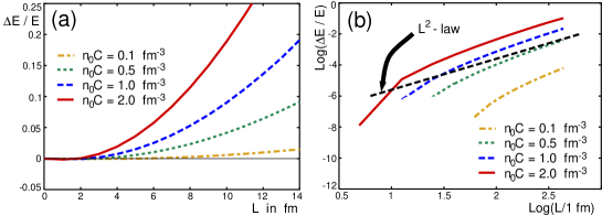
Figure 1: (a) Dependence of the medium-induced radiative energy loss $\langle\Delta E\rangle$ on the in-medium pathlength $L$ for $E=100$ GeV. The transport coefficient is defined here as $\frac{\hat{q}}{2}=n_{0}\,C$. (b) Double logarithmic presentation of (a). Figure taken from [60].

The limit $R\to\infty$ removes the kinematical constraint from (69) and coincides with the original result of Baier, Dokshitzer, Mueller, Peigné and Schiff[4],

$$\lim_{R\to\infty}\,\omega\frac{dI}{d\omega}=\frac{2\alpha_{s}C_{R}}{\pi}\,\ln\Bigg{|}{\cos\left[\,(1+i)\sqrt{\frac{\omega_{c}}{2\omega}}\,\right]}\Bigg{|}\,.$$ (88)

The limiting case for small $\omega$ is as expected from the estimates (86), [9]

$$\lim_{R\to\infty}\,\omega\frac{dI}{d\omega}\simeq\frac{2\alpha_{s}C_{R}}{\pi}\left\{\begin{array}[]{r@{\qquad\hbox{for}\quad}l}\sqrt{\frac{\omega_{c}}{2\,\omega}}&\omega<\omega_{c}\,,\\ \frac{1}{12}\left(\frac{\omega_{c}}{\omega}\right)^{2}&\omega>\omega_{c}\,.\end{array}\right.$$ (91)

The average parton energy loss is the zeroth moment of this energy distribution

$$\langle\Delta E\rangle_{R\to\infty}=\lim_{R\to\infty}\,\int d\omega\,\omega\frac{dI}{d\omega}\simeq\frac{\alpha_{s}C_{R}}{2}\,\omega_{c}\propto L^{2}\,.$$ (92)

This is the well-known $L^{2}$-dependence of the average energy loss [3, 4, 62]. The numerical calculation in Figure  1 shows deviations from the limiting case (92). [In Ref.[60], an erroneous prefactor $N_{c}$ was included in the definition of $\omega\frac{dI}{d\omega}$; hence, the values for $\Delta E$ shown in Fig.1 and 3 are a factor 3 too large.] In general, the strong increase of the average energy loss $\Delta E$ with in-medium pathlength indicates the strong sensitivity of partonic energy loss to the geometry of the nuclear collision.

Figure 2: The energy distribution of radiated gluons $\omega\frac{dI}{d\omega}$ for different values of the kinematical constraint $R=\omega_{c}\,L$. Figure taken from [52].

The average energy loss $\Delta E$ is the first moment of the energy distribution (69). Fig. 2 shows this distribution for finite values of the density parameter $R$. At sufficiently large gluon energy, the distribution approaches for any value of $R$ the BDMPS limit (88) . Below a critical gluon energy $\bar{\omega}$, however, the finite size gluon spectrum is depleted in comparison to the BDMPS limit. This suppression results from a phase space constraint: gluons are radiated on average at a characteristic angle [52],

$$\Theta_{c}^{2}\simeq\frac{k_{\perp}^{2}}{\omega^{2}}\simeq\frac{\sqrt{\omega\hat{q}}}{\omega^{2}}\simeq\left(\frac{\omega}{\omega_{c}}\right)^{-3/2}\frac{1}{R}<1\,.$$ (93)

This depletes the gluon distribution for gluon energy $\bar{\omega}$ below

$$\frac{\bar{\omega}}{\omega_{c}}\propto\left(\frac{1}{R}\right)^{2/3}\,.$$ (94)

This $R$-dependent suppression is seen clearly in Fig. 2.

Angular Dependence of the gluon energy distribution

Quantum Chromodynamics is a finite resolution theory; the energy of a single quark or gluon is not a measurable quantity. One rather measures the fraction of the hadronic decay products of a single quark or gluon which are radiated within a certain jet opening angle. Thus, the angular dependence of the medium-induced modification of gluon bremsstrahlung is important.

The angular dependence of $\omega\frac{dI}{d\omega}$ can be studied by varying the kinematic cut-off $\chi\,\omega$ of the transverse momentum integration [7, 60, 8]. For fixed characteristic gluon energy $\omega_{c}=\frac{1}{2}\hat{q}L^{2}$ and fixed dimensionless parameter $\frac{1}{2}\hat{q}L^{3}$, the radiation spectrum $\omega\frac{dI}{d\omega}$ inside a given angle $\Theta=\arcsin(\chi)$ depends on the parameters $\omega_{c}$ and $R=\chi^{2}\frac{1}{2}\hat{q}L^{3}$. From Fig. 2 one thus concludes immediately that the harder gluons are emitted more collinear.

From the gluon energy distribution inside a given cone opening angle, one obtains the medium-induced additional average energy emitted outside a cone of given opening angle $\Theta$,

$$\frac{\Delta E}{E}(\Theta=\arcsin(\bar{\chi}))=\frac{\Delta E}{E}(\chi=1)-\frac{\Delta E}{E}(\bar{\chi})\,.$$ (95)

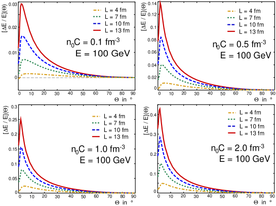
Figure 3: The fraction of the total radiative energy loss $\Delta E/E$ emitted outside a jet cone of fixed angle $\Theta$. Here, the transport coefficient is defined as $\hat{q}=2\,n_{0}\,C$. Figure taken from [60].

As seen from Fig. 3, $\frac{\Delta E}{E}(\Theta)$ does not decrease monotonously with increasing $\Theta$ but has a maximum at finite jet opening angle. The reason is that the radiative energy loss outside a cone angle $\Theta$ receives additional contributions from the Brownian $k_{\perp}$-broadening

$$\frac{1}{{\bf k}^{2}}\longrightarrow\frac{1}{({\bf k}+{\bf q})^{2}}$$ (96)

of the hard vacuum radiation term $I_{6}$. Such contributions do not affect the total ${\bf k}$-integrated yield $\frac{\Delta E}{E}(\Theta=0)$, since they result only in a shifting of the transverse momentum phase space distribution of the emitted gluon. However, this shift in transverse phase space shows up as soon as a finite cone size is chosen. We conclude from Fig. 3 that the total ${\bf k}$-integrated radiative energy loss$\frac{\Delta E}{E}(\Theta=0)$ is not the upper bound for the radiative energy loss outside a finite jet cone angle $\frac{\Delta E}{E}(\Theta)$. Depending on the transport coefficient and the in-medium path length, the latter can be larger by more than a factor $2$.

Harmonic oscillator approximation (expanding medium)

In nucleus-nucleus collisions at collider energies, the produced hard partons propagate through a rapidly expanding medium. The density of scattering centers and thus the transport coefficient $\hat{q}(\xi)$ is expected to reach a maximal value $\hat{q}_{d}$ around the plasma formation time $\xi_{0}$, and then decreases rapidly due to the strong longitudinal and - to a lesser extent - transverse expansion,

$$\hat{q}(\xi)=\hat{q}_{d}\left(\frac{\xi_{0}}{\xi}\right)^{\alpha}\,.$$ (97)

Here, $\alpha=0$ characterizes the static medium discussed above. The value $\alpha=1$ corresponds to a one-dimensional, boost-invariant longitudinal expansion and approximates the findings of hydrodynamical simulations. The formation time $\xi_{0}$ of the medium may be set by the inverse of the saturation scale $p_{\rm sat}$ [19] and is $\approx$ 0.2 fm/c at RHIC and $\approx$ 0.1 fm/c at LHC. Since the time difference between the formation of the hard parton and the formation of the medium bulk is irrelevant for the evaluation of the radiation spectrum (69), one can replace in (69) the production time $\xi_{0}$ of the parton by $0$.

For a dynamically evolving medium of the type (97), the path-integral (57) in (69) is the path integral of a 2-dimensional harmonic oscillator with time dependent (imaginary) frequency $\Omega^{2}(\xi)\equiv{\hat{q}(\xi)\over i2\omega}$ and mass $\omega$. The explicit solution can be written in terms of the variables $z(\xi)=2i\nu\Omega(\xi_{0})\xi_{0}\left({\xi\over\xi_{0}}\right)^{1/2\nu}$ and $\nu={1\over 2-\alpha}$: [5]

$${\cal K}({\bf r}(y_{l}),y_{l};{\bf r}(\bar{y}_{l}),\bar{y}_{l}|\omega)=$$ (98)

$${\omega\over 2\pi iD(\bar{y}_{l},y_{l})}\exp\left[-{\omega\over 2iD(\bar{y}_{l},y_{l})}\left(c_{1}{\bf r}(\bar{y}_{l})^{2}+c_{2}{\bf r}(y_{l})^{2}-2{\bf r}(\bar{y}_{l})\cdot{\bf r}(y_{l})\right)\right]\,.$$

Here, the coefficients are given by modified Bessel functions $I_{\nu}(z)$ and $K_{\nu}(z)$ [here: $z\equiv z(y_{l})$, $\bar{z}\equiv z(\bar{y}_{L})$]

$$c_{1} \equiv c_{1}(\bar{y}_{L},y_{L})=z(\bar{z}/z)^{\nu}\,\left[I_{\nu-1}(z)K_{\nu}(\bar{z})+K_{\nu-1}(z)I_{\nu}(\bar{z})\right]\,,$$ (99)

$$c_{2} \equiv c_{2}(\bar{y}_{L},y_{L})=\bar{z}(z/\bar{z})^{\nu}\,\left[K_{\nu}(z)I_{\nu-1}(\bar{z})+I_{\nu}(z)K_{\nu-1}(\bar{z})\right]\,.$$ (100)

and the fluctuation determinant reads

$$D(t,t_{0})={2\nu\xi_{0}\over(2i\nu\Omega(t_{o})\xi_{0})^{2\nu}}(zz_{0})^{\nu}\left[I_{\nu}(z)K_{\nu}(z_{0})-K_{\nu}(z)I_{\nu}(z_{0})\right]\,.$$ (101)

One checks that for $\alpha=0$, $\nu=\frac{1}{2}$, the solution (72) is regained.

Figure 4: LHS: The medium-induced gluon energy distribution radiation for a dynamically expanding collision regions (97) with expansion parameter $\alpha=$ 0, 0.5, 1.0 and 1.5. The value of the transport coefficient $\hat{q}_{0}$ is taken at initial time $\xi_{0}$. RHS: The same gluon radiation spectrum with parameters rescaled according to (102). Figure taken from [52].

Using the explicit form of the path integral (98), one can calculate the medium-induced gluon energy distribution (69) for a dynamically expanding medium [5]. The result is shown in Fig.4. The radiation spectrum $\omega\frac{dI}{d\omega}$ satisfies a simple scaling law which relates the radiation spectrum of a dynamically expanding collision region to an equivalent static scenario. The linearly weighed line integral [51]

$$\overline{\hat{q}}=\frac{2}{L^{2}}\int_{\xi_{0}}^{\xi_{0}+L}d\xi\,\left(\xi-\xi_{0}\right)\,\hat{q}(\xi)$$ (102)

defines the transport coefficient of the equivalent static scenario. The linear weight in (102) implies that scattering centers which are further separated from the production point of the hard parton are more effective in leading to partonic energy loss. In contrast to earlier believe that parton energy loss is most sensitive to the hottest and densest initial stage of the collision, this implies for a dynamical expansion following Bjorken scaling [$\alpha=1$ in eq. (97)] that all timescales contribute equally to the average transport coefficient. This makes partonic energy loss a valuable tool for the measurement of the quark-gluon plasma lifetime.

Properties of the transport coefficient

The only property of the medium which enters the medium-induced energy distribution (69) is the transport coefficient

$$\hat{q}=\mu^{2}/\lambda=\int\frac{d{\bf q}}{(2\pi)^{2}}\,{\bf q}^{2}\,|a_{+}({\bf q})|^{2}\,$$ (103)

For phenomenological estimates of the value $\hat{q}$ for cold nuclear matter, one often invokes the relation of $\hat{q}$ to the gluon structure function $\hat{q}=\frac{4\pi^{2}\,\alpha_{s}N_{c}}{N_{c}^{2}-1}\rho\left[xG(x,\hat{q}L)\right]$. This leads to estimates [4] $\hat{q}_{\rm cold}<(200\,{\rm MeV})^{2}/{\rm fm}$. There are alternative approaches [4, 1] which extract $\hat{q}_{\rm cold}$ from the medium modification of hard processes in “cold nuclear matter”, such as medium-modifications to the Drell-Yan production [1] in $p-A$ or the dijet imbalance in $e-A$ [43, 44]. The extracted values are consistent with $\hat{q}_{\rm cold}<(200\,{\rm MeV})^{2}/{\rm fm}$, but the systematic uncertainties of these determinations are difficult to specify.

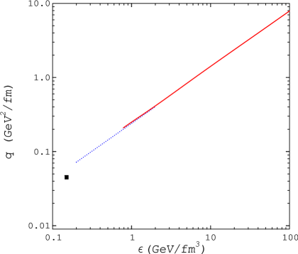
Figure 5: Estimate of the transport coefficient as a function of the energy density $\epsilon$. Figure taken from [10].

For the transport coefficient in hot quark-gluon matter, even less is known. Baier, Dokshitzer, Mueller and Schiff [4] estimated for the rescattering properties of hot matter at a temperature $T=250$ MeV a value $\hat{q}=(500\,{\rm MeV})^{2}/{\rm fm}$. In any case, the transport coefficient is expected to increase linearly with the energy density, as seen in Fig. 5. In the case of a phase transition at $T_{c}\approx 175$ MeV, this indicates a strong jump of $\hat{q}$ at $T_{c}$. The medium modification of hard processes observed at RHIC and LHC should allow to determine the value of $\hat{q}$ and thus provide an independent estimate of the energy density attained in the collision. For this, the proper treatment of the dynamical expansion of the collision region e.g. via (102) is obviously important.

The transport coefficient has been related also to the saturation momentum scale[10]

$$Q_{s}^{2}\simeq\hat{q}\,L\,.$$ (104)

The saturation scale entering here should be defined for a color octet dipole – thus, it is a factor $C_{A}/C_{F}$ larger than the saturation scale determined from the $q\bar{q}$ scattering probability in DIS. The numerical value of $Q_{s}$ is very uncertain but $Q_{s}^{2}\leq(3\,{\rm GeV})^{2}$ may be considered as an upper bound at LHC. For in-medium path lengths $L$ up to twice the nuclear size, this corresponds to values up to $R=\frac{1}{2}\hat{q}L^{3}<40000$.

2 Opacity Expansion of the radiation cross section

In what follows, we discuss the opacity expansion of the radiation cross section (69). This is based on the expansion of the path-integral (57) in powers of the dipole cross section,

$${\cal K}({\bf r},y_{l};{\bf\bar{r}},\bar{y}_{l})={\cal K}_{0}({\bf r},y_{l};{\bf\bar{r}},\bar{y}_{l})$$

$$-\int\limits_{z}^{z^{\prime}}\,{\it d}\xi\,n(\xi)\,\int{\it d}{\bf r}_{1}\,{\cal K}_{0}({\bf r},y_{l};{\bf r}_{1},\xi)\,\frac{1}{2}\,\sigma({\bf r}_{1})\,{\cal K}_{0}({\bf r}_{1},\xi;{\bf\bar{r}},\bar{y}_{l})$$

$$+\int\limits_{z}^{z^{\prime}}{\it d}\xi_{1}\,n(\xi_{1})\,\int\limits_{\xi_{1}}^{z^{\prime}}{\it d}\xi_{2}\,n(\xi_{2})\,\int{\it d}{\bf r}_{1}\,{\it d}{\bf r}_{2}\,{\cal K}_{0}({\bf r},y_{l};{\bf r}_{1},\xi_{1})\,$$

$$\times\frac{1}{2}\,\sigma({\bf r}_{1})\,{\cal K}({\bf r}_{1},\xi_{1};{\bf r}_{2},\xi_{2})\,\frac{1}{2}\,\sigma({\bf r}_{2})\,{\cal K}_{0}({\bf r}_{2},\xi_{2};{\bf\bar{r}},\bar{y}_{l})\,.$$ (105)

The $N$-th order in opacity is obtained by expanding the integrand of the gluon energy distribution (69) to $N$-th order in $\left(n(\xi)\,\sigma({\bf r})\right)^{N}$ [59, 26, 25]. We start with a discussion of the first order term for which the medium acts effectively as a single hard momentum transfer positioned within path length $L$.

Expansion to order $N=0$ and $N=1$

For the gluon energy distribution (69) of a free incoming quark, the zeroth order in opacity vanishes. A free incoming particle does not radiate without interaction. A parton produced in some hard process, however, does radiate without further interaction in order to decrease its virtuality. This is the DGLAP parton shower whose medium modification is accessed by the medium-induced spectrum $\omega\frac{dI}{d\omega}$. To zeroth order in $L\,n_{0}$, this spectrum is given by

$$\omega{d^{3}I(N=0)\over d\omega\,d{\bf k}}={\alpha_{s}\over\pi^{2}}\,C_{R}\,\frac{1}{{\bf k}^{2}}\,,\qquad H({\bf k})=\frac{1}{{\bf k}^{2}}\,,$$ (106)

(107)

This is the characteristic gluon radiation spectrum associated to the production of a hard parton. Medium modifications to (106) appear to first order in opacity. Introducing the transverse energies $Q=\frac{{\bf k}^{2}}{2\omega}$, $Q_{1}=\frac{\left({\bf k}+{\bf q}_{1}\right)^{2}}{2\omega}$, one finds

$$\omega{d^{3}I(N=1)\over d\omega\,d{\bf k}}={\alpha_{s}\over\pi^{2}}\,\frac{C_{R}}{2\,\omega^{2}}\,\int\frac{d{\bf q}_{1}}{(2\pi)^{2}}\,|a_{0}({\bf q}_{1})|^{2}$$

$$\qquad\qquad\qquad\times\frac{-{\bf k}\cdot{\bf q}_{1}}{Q\,Q_{1}}\,n_{0}\,\frac{LQ_{1}-\sin(LQ_{1})}{Q_{1}}\,.$$ (108)

(109)

The formation time for a medium-induced gluon is $t_{f}\approx 1/Q_{1}$. For a finite distance $\simeq L$ between the production point of the parton and the point of its rescattering, there are thus gluons whose formation times are too long: $L/t_{f}=LQ_{1}<1$. The interference term $\frac{LQ_{1}-\sin(LQ_{1})}{Q_{1}}$ in (108) prevents such gluons from being radiated. It provides a logarithmic cut-off for an otherwise infrared divergent ${\bf k}$- integrated expression, see eq. (121) below.

This radiation spectrum interpolates between the totally coherent and totally incoherent limiting cases. These can be discussed in terms of the isolated contributions for the hard (vacuum) and the medium-induced Gunion-Bertsch radiation terms:

(110)

In the totally coherent limit, the extension of the target is negligible, and medium-corrections are absent,

$$\lim_{L\to 0}{d^{3}\sigma^{(nas)}(N=1)\over d(\ln x)\,d{\bf k}}=0\,.$$ (111)

In the incoherent $L\to\infty$ limit, the radiation cross section (69) expanded up to first order in opacity, takes the form

$$\lim_{L\to\infty}\sum_{m=0}^{N=1}\omega{d^{3}I(m)\over d\omega\,d{\bf k}}={\alpha_{s}\over\pi^{2}}\,C_{F}(1-w_{1})H({\bf k})$$

$$\qquad+{\alpha_{s}\over\pi^{2}}\,C_{F}\,n_{0}\,L\,\int\frac{d{\bf q}_{1}}{(2\pi)^{2}}|a_{0}({\bf q}_{1})|^{2}\Bigg{(}H({\bf k}+{\bf q}_{1})+R({\bf k},{\bf q}_{1})\Bigg{)}\,.$$ (112)

The three terms on the r.h.s. of (112) have a simple physical meaning: the first is the hard, medium-independent radiation (106) reduced by the probability $w_{1}$ that one interaction of the projectile occurs in the medium. The second term describes the hard radiation component which rescatters once in the medium. The third term is the medium-induced Gunion-Bertsch contribution associated with the rescattering. For the case $N=1$, the above discussion that eq. (108) pattern interpolates between simple and physically intuitive limiting cases. In general, the $N$-th order term in the opacity expansion is a convolution of the radiation associated to $N$-fold scattering and a readjustment of the probabilities that rescattering occurs with less than $N$ scattering centers [59].

Qualitative estimates of $\omega\frac{dI}{d\omega}$ vs. quantitative calculations

In general, the radiation spectrum $\omega\frac{dI}{d\omega}$ displays an interference pattern between medium-induced and hard (vacuum) radiation amplitudes. Formation time effects determine this interplay and allow for some qualitative estimates. In the simplest case, consider a hard partonic projectile which picks up a single transverse momentum $\mu$ by interacting with a single hard scatterer. An additional gluon of energy $\omega$ decoheres from the projectile wave function if its typical formation time $\bar{t}_{\rm coh}=\frac{2\omega}{\mu^{2}}$ is smaller than the typical distance $L$ between the production point of the parton and the position of the scatterer. The relevant phase is

$$\gamma=\frac{L}{\bar{t}_{\rm coh}}\equiv\frac{\bar{\omega}_{c}}{\omega}\,.$$ (113)

Thus one expects that the radiation of gluons is suppressed if their energy $\omega$ is larger than the characteristic gluon energy

$$\bar{\omega}_{c}=\frac{1}{2}\mu^{2}\,L\,.$$ (114)

From this one can estimate the gluon energy spectrum per unit path length in terms of the coherence time $\bar{t}_{\rm coh}$,

$$\omega\frac{dI^{N=1}}{d\omega\,dz}\simeq\frac{\alpha_{s}}{\bar{t}_{\rm coh}}\simeq\alpha_{s}\,\frac{\mu^{2}}{\omega}\,.$$ (115)

This estimate can be compared to the full $N=1$ opacity term (108) integrated over transverse momentum up to $|{\bf k}|<\chi\,\omega$. Introducing the kinematic constraint in transverse momentum phase space,

$$\bar{R}=\chi^{2}\bar{\omega}_{c}\,L\,,$$ (116)

the gluon radiation spectrum takes the form[52]

$$\omega\frac{dI^{N=1}}{d\omega} = 2\frac{\alpha_{s}\,C_{R}}{\pi}\,(n_{0}L)\,\gamma\,\int_{0}^{\infty}dr\,\frac{r-sin(r)}{r^{2}}$$ (117)

$$\times\left(\frac{1}{r+\gamma}-\frac{1}{\sqrt{((\bar{R}/2\gamma)+r+\gamma)^{2}-4r\bar{R}/2\gamma}}\right)\,.$$

Figure 6: The medium-induced gluon energy distribution $\omega\frac{dI}{d\omega}$ in the $N=1$ opacity expansion. Different curves are for different values of the kinematic constraint $\bar{R}=\bar{\omega}_{c}\,L$. Figure taken from [52].

The expression (117) is plotted in Fig. 6. It shows qualitatively the same shape as the spectrum in the multiple soft scattering case. The position of the maximum of $\omega\frac{dI(N=1)}{d\omega}$ changes $\propto\frac{1}{\sqrt{\bar{R}}}$. This is in accordance with the assumption that gluon radiation is suppressed for energies below which the characteristic angle of the gluon emission is of order one

$$\Theta_{c}^{2}\simeq\frac{\mu^{2}}{\omega^{2}}\simeq\left(\frac{\bar{\omega}_{c}}{\omega}\right)^{2}\frac{1}{\bar{R}}\sim 1\quad\Longrightarrow\quad\frac{\omega}{\bar{\omega}_{c}}\propto\frac{1}{\sqrt{\bar{R}}}\,.$$ (118)

In the limit $\bar{R}\to\infty$ in which the phase space constraint is removed, one recovers some pocket formulas from the literature [25]. First, this limit satisfies the characteristic $1/\omega$-energy dependence of the estimate (115) for sufficiently large gluon energies $\omega>\bar{\omega}_{c}$,

$$\lim_{\bar{R}\to\infty}\,\omega\frac{dI(N=1)}{d\omega} = 2\,\frac{\alpha_{s}\,C_{R}}{\pi}\,\left(n_{0}\,L\right)\,\gamma\,\int_{0}^{\infty}dr\,\frac{1}{r+\gamma}\,\frac{r-sin(r)}{r^{2}}\,$$ (121)

$$\simeq 2\,\frac{\alpha_{s}\,C_{R}}{\pi}\,\left(n_{0}\,L\right)\,\left\{\begin{array}[]{r@{\qquad\hbox{for}\quad}l}\log\left[\frac{\bar{\omega}_{c}}{\omega}\right]&\bar{\omega}_{c}>\omega\\ \frac{\pi}{4}\,\frac{\bar{\omega}_{c}}{\omega}&\bar{\omega}_{c}<\omega\end{array}\right.$$

Moreover, this expression allows to estimate the average parton energy loss for a single hard scattering. Remarkably, this seems dominated by contributions from the region $\omega>\bar{\omega}_{c}$,[25, 66]

$$\lim_{\bar{R}\to\infty}\langle\Delta E\rangle^{N=1}=\lim_{\bar{R}\to\infty}\,\int d\omega\,\omega\frac{dI^{N=1}}{d\omega}\simeq\frac{\alpha_{s}C_{R}}{2}(n_{0}L)\,\bar{\omega}_{c}\,\log\left[E/\bar{\omega}_{c}\right]\,,$$ (122)

which appears to be logarithmically enhanced in comparison to the region $\omega<\bar{\omega}_{c}$ for which

$$\lim_{\bar{R}\to\infty}\,\int_{0}^{\bar{\omega}_{c}}d\omega\,\omega\frac{dI^{N=1}}{d\omega}\simeq\frac{2\,\alpha_{s}C_{R}}{\pi}(n_{0}L)\,\bar{\omega}_{c}\,.$$ (123)

However, the logarithmic enhancement of (122) does not persist upon closer inspection: All calculations so far worked for fixed coupling constant which may be justified if all momentum transfers are of the same order. In calculating (122), however, the ${\bf k}$-integration was extended up to the total energy $E$. If one takes the running of the coupling into account, this logarithmic enhancement factor is reduced to a $\log\log$ factor.

Parameters in the opacity expansion

In the multiple scattering approximation, the gluon energy distribution (69) depends on two quantities: the transport coefficient $\hat{q}$ and the in-medium path length $L$ (we ignore the angular dependence in the following discussion). In the opacity expansion, there are three parameters instead: the in-medium path length $L$, the transverse momentum squared $\mu^{2}$ transferred on average by a single scattering, and the inverse mean free path $n_{0}=\frac{1}{\lambda}$. The multiple scattering approximation describes the average momentum transfer per unit path length while the opacity expansion specifies in addition by how many scattering centers this momentum is transferred on average. In the limit of multiple soft scattering, this additional information is redundant since

$$\mu^{2}\,n_{0}\,L=\hat{q}\,L\,,\qquad\hbox{for Brownian motion.}$$ (124)

However, deviations from Brownian motion arise due to the high transverse momentum tails of the elastic scattering cross sections $|a({\bf q})|^{2}=\left(\mu^{2}(2\pi)^{2}\right)/\left({\pi({\bf q}^{2}+\mu^{2})^{2}}\right)$. These tails lead to a logarithmically enhancement factor in the transport coefficient

$$\hat{q}\,L=n_{0}L\int^{Q}\frac{d^{2}{\bf q}}{(2\pi)^{2}}\,|a({\bf q})|^{2}\,\frac{1}{2}\,{\bf q}^{2}\,\cos^{2}\varphi\sim(n_{0}L)\,\mu^{2}\,\ln\sqrt{\frac{Q}{\mu}}\,.$$ (125)

This allows to relate via $\omega_{c}\simeq(n_{0}L)\,\bar{\omega_{c}}\ln\sqrt{\frac{Q}{\mu}}$ the characteristic gluon energies (85) and (114) which set the energy scale in the multiple soft and single hard scattering limits. For realistic values [$\mu\geq\Lambda_{\rm QCD}$ and $Q\leq E$ say], $\ln\sqrt{\frac{Q}{\mu}}\ll 10$, one concludes from Figs. 1 and  6 that the medium-induced gluon energy distribution is significantly harder in the opacity approximation than in the multiple soft scattering limit[52].

5 Applications

Irrespective of the number of additionally radiated gluons, what matters for the medium modification of hadronic observables is how much additional energy $\Delta E$ is radiated off a hard parton. In this section, we first discuss the so called quenching weight which is the probability distribution $P(\Delta E)$ of the additional medium-induced energy loss. For independent gluon emission, this probability is the normalized sum of the emission probabilities for an arbitrary number of $n$ gluons which carry away a total energy $\Delta E$:[9]

$$P(\Delta E)=\sum_{n=0}^{\infty}\frac{1}{n!}\left[\prod_{i=1}^{n}\int d\omega_{i}\frac{dI(\omega_{i})}{d\omega}\right]\delta\left(\Delta E-\sum_{i=1}^{n}\omega_{i}\right)e^{-\int d\omega\frac{dI}{d\omega}}\,.$$ (126)

Then we discuss how this probability can be used to calculate the medium modification of hadronic observables.

1 Properties of Quenching Weights

In general, the quenching weight (126) has a discrete and a continuous part,[51]

$$P(\Delta E)=p_{0}\,\delta(\Delta E)+p(\Delta E)\,.$$ (127)

The discrete weight $p_{0}$ emerges as a consequence of a finite mean free path. It determines the probability that no additional gluon is emitted due to in-medium scattering and hence no medium-induced energy loss occurs.

In order to determine the discrete and continuous part of (127), it is convenient to rewrite eq. (126) as a Laplace transformation [9]

$$P(\Delta E) = \int_{C}\frac{d\nu}{2\pi i}\,{\cal P}(\nu)\,e^{\nu\Delta E}\,,$$ (128)

$${\cal P}(\nu) = \exp\left[-\int_{0}^{\infty}d\omega\,\frac{dI(\omega)}{d\omega}\,\left(1-e^{-\nu\,\omega}\right)\right]\,.$$ (129)

Here, the contour $C$ runs along the imaginary axis with ${\rm Re}\nu=0$.

For the further discussion, it is useful to treat the medium-induced gluon energy distribution $\omega\frac{dI}{d\omega}$ in eq. (69) explicitly as the medium modification of a “vacuum” distribution [52]

$$\omega\frac{dI^{({\rm tot})}}{d\omega}=\omega\frac{dI^{({\rm vac})}}{d\omega}+\omega\frac{dI}{d\omega}\,.$$ (130)

From the Laplace transform (128), one finds the total probability

$$P^{({\rm tot})}(\Delta E)=\int_{0}^{\infty}d\bar{E}\,P(\Delta E-\bar{E})\,P^{({\rm vac})}(\bar{E})\,.$$ (131)

This probability $P^{({\rm tot})}(\Delta E)$ is normalized to unity and it is positive definite. In contrast, the medium-induced modification of this probability, $P(\Delta E)$, is a generalized probability. It can take negative values for some range in $\Delta E$, as long as its normalization is unity,

$$\int_{0}^{\infty}d\bar{E}\,P(\bar{E})=p_{0}+\int_{0}^{\infty}d\bar{E}\,p(\bar{E})=1\,.$$ (132)

We now discuss separately the properties of the discrete contribution $p_{0}$ and the continuous one $p(\bar{E})$. A CPU-inexpensive Fortran routine[52] is available for the calculation of these quenching weights.

Figure 7: The discrete part $p_{0}$ of the quenching weight calculated in the multiple soft scattering limit as a function of $R$. Figure taken from [52].

Discrete part of the quenching weight

The discrete part of the quenching weight is the $n=0$ term of eq. (126). It can be expressed in terms of the total gluon multiplicity,

$$p_{0}=\lim_{\nu\to\infty}\,{\cal P}(\nu)=\exp\left[-N(\omega=0)\right]\,,$$ (133)

where the multiplicity $N(\omega)$ of gluons with energy larger than $\omega$ emerges by partially integrating the exponent of (129),

$$N(\omega)\equiv\int_{\omega}^{\infty}d\omega^{\prime}\,\frac{dI(\omega^{\prime})}{d\omega^{\prime}}\,.$$ (134)

For the limiting case of infinite in-medium path length, the total multiplicity $N(\omega)$ diverges and the discrete part vanishes. In general, however, $p_{0}$ is finite. A typical dependence of $p_{0}$ on model parameters is shown in Fig. 7 for the radiation spectrum calculated in the multiple soft scattering limit. A qualitatively similar behavior is found in the opacity expansion. Remarkably, $p_{0}$ can exceed unity for some parameter range, since the medium modification $\omega\frac{dI}{d\omega}$ to the radiation spectrum (130) can be negative. The value $p_{0}>1$ then compensates a predominantly negative continuous part $p(\Delta E)$ and satisfies the normalization (132). This indicates a phase space region at very small transverse momentum, into which less gluons are emitted in the medium than in the vacuum. This effect is more pronounced for gluons than for quarks.

Continuous part of the quenching weight

The continuous part $p(\Delta E)$ of the probability distribution (127) can be calculated numerically from the Mellin transform (129). To facilitate the numerical calculation, one subtracts from $P(\nu)$ the discrete contribution $p_{0}$ which dominates the large-$\nu$ behavior.

Fig. 8 shows the continuous part of the quenching weight, calculated in the multiple soft scattering limit. In the opacity expansion, it looks qualitatively similar. As expected from the normalization condition (132), the continuous part $p(\Delta E)$ shows predominantly negative contributions for the parameter range for which the discrete weight $p_{0}$ exceeds unity. With increasing density of scattering centers (i.e. increasing $R=\frac{1}{2}\hat{q}L^{3}$) the probability of loosing a significant energy fraction $\Delta E$ increases. The energy loss is larger for gluons which have a stronger coupling to the medium. This broadens the width of $p(\Delta E)$ for the gluonic case.

Figure 8: The continuous part of the quenching weight (127), calculated in the multiple soft scattering limit for a hard quark (upper row) or hard gluon (lower row). Figure taken from [52].

In the multiple soft scattering approximation, an analytic estimate for the quenching weight can be obtained[9] in the limit $R\to\infty$ from the small-$\omega$ approximation $\omega\frac{dI}{d\omega}\propto\frac{1}{\sqrt{\omega}}$

$$P^{\rm approx}_{\rm BDMS}(\epsilon)=\sqrt{\frac{a}{\epsilon^{3}}}\exp\left[-\frac{\pi\,a}{\epsilon}\right]\,,\qquad\hbox{\rm where}\,\,a=\frac{2\,\alpha_{s}^{2}\,C_{R}^{2}}{\pi^{2}}\omega_{c}\,.$$ (135)

This reproduces roughly [51] the shape of the probability distribution for large system size, but it has an unphysical large $\epsilon$-tail with infinite first moment $\int d\epsilon\,\epsilon\,P^{\rm approx}_{\rm BDMS}(\epsilon)$. An alternative analytic approach [2] aims at fitting a two-parameter log-normal distribution to the numerical result for $P(\Delta E)$.

2 Quenching factors for hadronic spectra

Assume that a hard parton looses an additional energy fraction $\Delta E$ while escaping the collision region. The medium-dependence of the corresponding inclusive transverse momentum spectra can be characterized in terms of the quenching factor $Q$ [9]

$$Q(p_{\perp}) = {{d\sigma^{\rm med}(p_{\perp})/dp^{2}_{\perp}}\over{d\sigma^{\rm vac}(p_{\perp})/dp^{2}_{\perp}}}=\int d{\Delta E}\,P(\Delta E)\left({d\sigma^{\rm vac}(p_{\perp}+\Delta E)/dp^{2}_{\perp}}\over{d\sigma^{\rm vac}(p_{\perp})/dp^{2}_{\perp}}\right)$$ (136)

$$\simeq \int d{\Delta E}\,P(\Delta E)\,\left({p_{\perp}\over p_{\perp}+\Delta E}\right)^{n}\,.$$

Here, the last line is obtained by assuming a power law fall-off of the $p_{\perp}$-spectrum. The effective power $n$ depends in general on $p_{\perp}$. It is $n\simeq 7$ for the $p_{\perp}$-range relevant for RHIC. Alternatively, instead of the quenching factor (136), the medium modification of hadronic transverse momentum spectra is often characterized by a shift factor $S(p_{\perp})$,

$$\frac{d\sigma^{{\rm med}}(p_{\perp})}{dp^{2}_{\perp}}\simeq\frac{d\sigma^{{\rm vac}}(p_{\perp}+S(p_{\perp}))}{dp^{2}_{\perp}}\,,$$ (137)

which is related to the shift $S(p_{\perp})$ by

$$Q(p_{\perp})=\exp\left\{-\frac{n}{p_{\perp}}\cdot S(p_{\perp})\right\}\,.$$ (138)

Most importantly, since the hadronic spectrum shows a strong power law decrease, what matters for the suppression is not the average energy loss $\langle\Delta E\rangle$ but the least energy loss with which a hard parton is likely to get away. One concludes that $S(p_{\perp})<\langle\Delta E\rangle$ and depends on transverse momentum [9].

Figure 9: The quenching factor (136) calculated in the multiple soft scattering limit. Upper row: calculation in the $R\to\infty$-limit but with a variable sharp cut-off on the infrared part of the gluon energy distribution. Lower row: the same calculation is insensitive to infrared contributions if the finite kinematic constraint $R=\omega_{c}L<\infty$ is included. Figure taken from [52].

Fig. 9 shows a calculation of the quenching factor (136) in the multiple soft scattering limit. A qualitatively similar result is obtained in the opacity expansion. In general, quenching weights increase monotonically with $p_{\perp}$ since the medium-induced gluon radiation is independent of the total projectile energy for sufficiently high energies. At very low transverse momenta, the calculation based on (69) is not reliable and the interpretation of the medium modification of hadronic spectra in nucleus-nucleus collisions will require additional input (e.g. modifications due to the Cronin effect). Fig. 9 suggests, however, that hadronic spectra at transverse momenta $p_{\perp}>10$ GeV, can be suppressed significantly due to partonic final state rescattering.

To quantify the sensitivity of the calculation to the low momentum region, Baier et al.[9] introduced a sharp cut-off on the $R\to\infty$ gluon energy distribution which was varied between $\omega_{\rm cut}=0$ and $\omega_{\rm cut}=500$ MeV. However, phase space constraints (i.e. finite $R$) deplete the gluon radiation spectrum in the soft region, see Fig. 2. As seen in Fig. 9, this decreases significantly the sensitivity of quenching factors to the uncontrolled infrared properties of the radiation spectrum.

3 Medium-modified fragmentation functions

For an alternative calculation of the medium modification of hadronic spectra, one may determine the dependence of fragmentation functions on partonic energy loss. In general, hadronic cross sections are calculated by convoluting the parton distributions of the incoming projectiles with the product $d\sigma^{h}(z,Q^{2})$ of a perturbatively calculable partonic cross section $\sigma^{q}$ and the fragmentation function $D_{h/q}(x,Q^{2})$ of the produced parton, $d\sigma^{h}(z,Q^{2})=\left(\frac{d\sigma^{q}}{dy}\right)dy\,D_{h/q}(x,Q^{2})\,dx$. Here, $x=E_{h}/E_{q}$, $y=E_{q}/Q$ and $z=E_{h}/Q$ denote fractions between the virtuality of the hard process $Q$, and the energies of the produced parton and resulting hadron. If the produced parton loses with probability $P(\epsilon)$ an additional fraction $\epsilon=\frac{\Delta E}{E_{q}}$ of its energy due to medium-induced radiation, then the hadronic cross section is given in terms of the medium-modified fragmentation function [54, 28]

$$D_{h/q}^{(\rm med)}(x,Q^{2})=\int_{0}^{1}d\epsilon\,P(\epsilon)\,\frac{1}{1-\epsilon}\,D_{h/q}(\frac{x}{1-\epsilon},Q^{2})\,.$$ (139)

The hadronized remnants of the medium-induced soft radiation are neglected in the definition of (139). However, these remnants are expected to be soft, and their inclusion would thus amount to an additional contribution to $D_{h/q}^{(\rm med)}(x,Q^{2})$ for $x>0.1$ say.

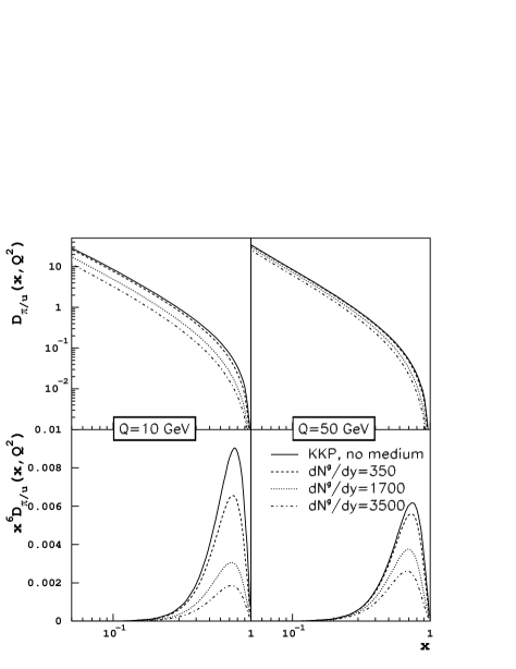
Figure 10: The LO KKP [31] fragmentation function $u\to\pi$ for no medium and the medium-modified fragmentation functions for different gluon rapidity densities (see eq. (140)) and $L=7$ fm. Figure taken from [51].

Fig. 10 shows a calculation of the parton fragmentation functions $D_{\pi/q}(x,Q^{2})$ from (139) using the quenching weights of Fig. 8 and the LO KKP [31] parametrization of $D_{h/q}(x,Q^{2})$. For this calculation, the virtuality $Q$ of $D_{h/q}(x,Q^{2})$ is identified with the (transverse) initial energy $E_{q}$ of the parton. This is justified since $E_{q}$ and $Q$ are of the same order, and $D_{h/q}(x,Q^{2})$ has a weak logarithmic $Q$-dependence while medium-induced effects change as a function of $\epsilon=\frac{\Delta E}{Q}\approx O(\frac{1}{Q})$. For a collision region expanding according to Bjorken scaling, the transport coefficient can be related to the initial gluon rapidity density [4, 27],

$$R=\frac{1}{2}\hat{q}L^{3}=\frac{L^{2}}{R_{A}^{2}}\,\frac{dN^{g}}{dy}\,.$$ (140)

That’s what is done in Fig. 10. Interestingly, eq. (140) indicates how partonic energy loss changes with the particle multiplicity in nucleus-nucleus collisions. This allows to extrapolate parton energy loss effects from RHIC to LHC energies [51].

In principle, the medium modified fragmentation function should be convoluted with the hard partonic cross section and parton distribution functions in order to determine the medium modified hadronic spectrum. For illustration, however, one may exploit that hadronic cross sections weigh $D_{h/q}^{(\rm med)}(x,Q^{2})$ by the partonic cross section ${d\sigma^{q}}/{dp_{\perp}^{2}}\sim{1}/{p_{\perp}^{n(\sqrt{s},p_{\perp})}}$ and thus effectively test $x^{n(\sqrt{s},p_{\perp})}D_{h/q}^{(\rm med)}(x,Q^{2})$ [20]. The value $n=6$ characterizes [20] the power law for typical values at RHIC ($\sqrt{s}=200$ GeV and $p_{\perp}\sim 10$ GeV). Thus, the position of the maximum $x_{\rm max}$ of $x^{6}D_{h/q}^{(\rm med)}(x,Q^{2})$ corresponds to the most likely energy fraction $x_{\rm max}E_{q}$ of the leading hadron. And the suppression around its maximum translates into a corresponding relative suppression of this contribution to the high-$p_{\perp}$ hadronic spectrum at $p_{\perp}\sim x_{\rm max}E_{q}$. In general, the suppression of hadronic spectra extracted in this way is in rough agreement[52] with calculations of the quenching factor (136).

6 Appendix A: Eikonal calculations in the target light cone gauge.

In section 2 of this review we have used the light cone gauge $A^{-}=0$. In this gauge the gluon and quark distributions of the projectile wave function are simply expressible in terms of the gluon and quark number operators and we will therefore refer to it as the projectile light cone gauge (PLCG). The standard light cone gauge used in DIS calculations on the other hand is $A^{+}=0$, which facilitates simple expressions of the target distribution functions. In this appendix we show how the spectrum of emitted gluons is obtained in this standard light cone gauge, which we will refer to as the target light cone gauge (TLCG).

Recall, that in PLCG the target is described as an ensemble of gluon fields with dominant component $A^{+}$. The eikonal $S$-matrix for the propagation of a charged parton through the target is given my the Wilson line eq.(3)

$$W({\bf x}_{i})={\cal P}\exp\{i\int dz_{-}T^{a}A^{+}_{a}({\bf x}_{i},z_{-})\}$$ (141)

In the TLCG the $A^{+}$ component of the vector potential vanishes. Instead the chromoelectric fields in the target are given in terms of the transverse components $A_{i}$. The $A^{i}$ are obtained from $A^{+}$ by the gauge transformation from PLCG to TLGT [37]

$$A_{i}({\bf x}_{i},x_{-})=iV^{\dagger}({\bf x}_{i},x_{-})\partial_{i}V({\bf x}_{i},x_{-})$$ (142)

where

$$V({\bf x}_{i},x_{-})={\cal P}\exp\{i\int_{-\infty}^{x_{-}}dz_{-}T^{a}A^{+}_{a}({\bf x}_{i},z_{-})\}$$ (143)

Note that the TLGT condition $A^{+}=0$ does not fix the gauge unambiguously, but only up to residual gauge transformation which does not depend on $x^{-}$. The choice of the lower limit of the $z_{-}$ integration in eq.(143) is equivalent to fixing this residual gauge freedom by imposing the condition $\partial_{j}A_{j}({\bf x}_{i},x_{-}\rightarrow-\infty)=0$ [37]. With this choice we have

$$V({\bf x}_{i},x_{-}\rightarrow-\infty)=1,\ \ \ \ V({\bf x}_{i},x_{-}\rightarrow\infty)=W({\bf x}_{i})\,.$$ (144)

Eq.(142) defines the vector potential $A_{i}$ as two dimensional pure gauge, $\partial_{i}A^{a}_{j}-\partial_{j}A^{a}_{i}-f^{abc}A^{b}_{i}A^{c}_{j}=0$. Moreover, at $x_{-}\rightarrow+\infty$ the vector potential is genuinely (and not just two dimensionally) pure gauge.

Let us now consider scattering of a projectile with the wave function eq.(1) on the target described by ensemble of fields $A_{i}$ of the form eq.(142). Since the $A^{+}$ component of the vector potential vanishes, in eikonal approximation the wave function of the projectile does not change while it propagates through the target. The outgoing wave function therefore is equal to the incoming one

$$\Psi_{out}=\sum_{\{\alpha_{i},{\bf x}_{i}\}}\,\psi(\{\alpha_{i},{\bf x}_{i}\})\,|\{\alpha_{i},{\bf x}_{i}\}\rangle\,.$$ (145)

This however does not mean that no scattering takes place. To calculate the scattering amplitude one has to project the outgoing wave function into the Hilbert space orthogonal to the wave function of the freely propagating system far ”to the right” of the target, that is at $x_{-}\rightarrow+\infty$. In the PLCG the target gauge field vanishes at both $x_{-}\rightarrow-\infty$ and $x_{-}\rightarrow+\infty$ and the freely propagating wave functions are identical ”to the left” and ”to the right” of the target. However in TLGT this is not the case. At $x_{-}\rightarrow+\infty$ the target vector potential does not vanish, but is instead a pure gauge, eq. (142). Therefore the freely propagating wave function at $x_{-}\rightarrow+\infty$ is not identical to that at $x_{-}\rightarrow-\infty$, but is rather its gauge transform with the gauge transformation generated by the Wilson loop eq. (141). In particular the fields ”to the right” of the target, $A$ are related to the fields ”to the left” of the target, $a$ by

$$A=W^{\dagger}aW+iW^{\dagger}\partial W\,.$$ (146)

Thus the free Fock basis ”to the right” of the target is related to the free Fock basis ”to the left” of the target by

$$|\{\alpha,{\bf x}_{i}\}\rangle_{R}=W^{\dagger}_{\alpha\beta}({\bf x}_{i})|\{\beta,{\bf x}_{i}\}\rangle_{L}\ .$$ (147)

The outgoing wave function eq.(145) is given in the basis $|\{\alpha,{\bf x}_{i}\}\rangle_{L}$. On the other hand all observables at late time after scattering, including the number of emitted gluons must be calculated with respect to the basis $|\{\alpha,{\bf x}_{i}\}\rangle_{R}$. It is thus convenient to rewrite $\Psi_{out}$ using eq.(147) as

$$\Psi_{out}=\sum_{\{\alpha_{i},{\bf x}_{i}\}}\psi(\{\alpha_{i},{\bf x}_{i}\})\prod_{i}W({\bf x}_{i})_{\alpha_{i}\beta_{i}}\,|\{\beta_{i},{\bf x}_{i}\}\rangle_{R}\,.$$ (148)

However the same projectile freely propagating to the right of the target would have the wave function

$$\Psi_{free}=\sum_{\{\alpha_{i},{\bf x}_{i}\}}\,\psi(\{\alpha_{i},{\bf x}_{i}\})\,|\{\alpha_{i},{\bf x}_{i}\}\rangle_{R}\,.$$ (149)

Thus we see that the outgoing wave function indeed differs from the freely propagating one, and thus the scattering is nontrivial and gluons are emitted in the final state. It is a somewhat curious feature of the TLCG that the nontrivial scattering amplitude appears entirely due to rotation of the free particle basis between early and late times Nevertheless it is obvious that the results of the calculation in this gauge are identical to those in PLCG as they should be. In fact from this point on all calculations are identical to those presented in section 2, as the interesting part of the outgoing wave function is given by eq.(5) with $\Psi_{free}$ of eq.(149) substituted for $\Psi_{in}$ and the ”free” gluons are defined as states in the $R$ Hilbert space, $|\{\alpha,{\bf x}\}\rangle_{R}$.

7 Appendix B: Path integral formalism for the photon radiation spectrum

In section 3, we discussed how to derive the non-abelian gluon radiation spectrum from the non-abelian Furry approximation (1). In this appendix, we present in more detail the derivation of the abelian analogue from the abelian Furry wave function (50). The QED photon radiation cross section in terms of Furry wave functions reads[57]

$$\frac{d^{5}\sigma}{d({\rm ln}x)\,d{\bf p}\,d{\bf k}}=\frac{\alpha_{em}}{(2\pi)^{4}}\,\left|M_{fi}\right|^{2}\,,$$ (150)

$$M_{fi}=\int d^{4}x\,{\Psi^{-}}^{\dagger}(x,p_{2})\,{\bf\alpha}\cdot{\bf\epsilon}\,e^{-\epsilon\,|z|}\,e^{i\,k\cdot x}\,\Psi^{+}(x,p_{1})\ .$$ (151)

Here, $e^{-\epsilon\,|z|}$ is the adiabatic switching off of the interaction term at large distances, discussed below eq. (64). To simplify (151), we perform the following steps:

1. Rotation of coordinate system Choose the momenta $p_{1}$ and $p_{2}$ of the incoming and outgoing electron in the frame in which the longitudinal axis is taken along the photon:

   $${\bf p}_{1} = {-1\over x}\,{\bf k}\,,\qquad{\bf p}_{2}={\bf p}-{1-x\over x}\,{\bf k}\,,$$ (152)

2. z-dependent phase: The z-dependent phases of the Furry wave function (50) combine in the radiation amplitude (151) to an inverse photon formation length

   $$\bar{q}=p_{1}-p_{2}-k=\frac{x\,m_{e}^{2}}{2\,(1-x)\,E_{1}}\,.$$ (153)

3. Simplifying the spinor structure: The spinor structure

   $$\widehat{\Gamma}_{r}=\sqrt{1-x}\,u^{*}({\bf p}_{2})\,\hat{D}^{*}_{2}\,{\bf\alpha}\cdot{\bf\epsilon}\,\hat{D}_{1}\,u({\bf p}_{1})$$ (154)

   in the amplitude (151) can be simplified on the cross section level. The spin- and helicity-averaged combination $\widehat{\Gamma}_{r}\,\widehat{\Gamma}_{r^{\prime}}^{*}$ take the simple form

   $$\widehat{\Gamma}_{r}\,\widehat{\Gamma}_{r^{\prime}}^{*}=\left[4-4x+2x^{2}\right]\frac{\partial}{\partial{\bf r}}\cdot\frac{\partial}{\partial{\bf r^{\prime}}}\,+2m_{e}^{2}x^{2}\,.$$ (155)

4. in-medium average: The cross section (150) contains products of the Green’s functions (58). These are averaged over the distribution of scattering centers in the medium, see (52) for the non-abelian case. These averages can be written in terms of the dipole cross section (14):

   $$\Bigg{\langle}\exp\left\{i\int\limits_{z}^{z^{\prime}}{\it d}\xi\,\left[U\bigl{(}{\bf r}(\xi),\xi\bigr{)}-U\bigl{(}{\bf r}^{\prime}(\xi),\xi\bigr{)}\right]\right\}\Bigg{\rangle}$$

   $$\qquad=\exp\left\{-\frac{1}{2}\int\limits_{z}^{z^{\prime}}{\it d}\xi\,n(\xi)\,\sigma\bigr{(}{\bf r}(\xi)-{\bf r}^{\prime}(\xi)\bigl{)}\right\}\,.$$ (156)

   For the products of Green’s functions, this leads to

   $$\langle G(\rho,z^{\prime};{\bf r},z|p_{2})\,\,G^{*}({\bf r}^{\prime},z^{\prime};\rho^{\prime},z|p_{1})\,\rangle=\frac{-p}{2\pi\,i\,(z^{\prime}-z)}\frac{1}{x}$$

   $$\times\exp\left\{\frac{ip}{2\,(z^{\prime}-z)}\left[(1-x)\bigl{(}\rho-{\bf r}\bigr{)}^{2}-\bigl{(}{\bf r}^{\prime}-\rho^{\prime}\bigr{)}^{2}\right]\right\}$$

   $$\times\int{\cal D}{\bf r}_{b}\exp\left\{\frac{i\mu}{2}\int_{z}^{z^{\prime}}{\dot{\bf r}}_{b}^{2}-\int_{z}^{z^{\prime}}\Sigma\bigl{(}\xi,{\hat{\rho}}_{f}+x{\bf r}_{b}\bigr{)}\right\}\,,$$ (157)

   where $\mu=p\,(1-x)\,x$ and

   $${\hat{\rho}}_{f}(\xi)={\rho}_{2}\frac{\xi-z}{z^{\prime}-z}+{\rho}_{1}\frac{z^{\prime}-\xi}{z^{\prime}-z}\,.$$ (158)

After inserting the Furry wave function (50) into the radiation amplitude (151). The radiation probability $\langle|M_{fi}|^{2}\rangle$ in terms of averages of Green’s functions reads

$$\langle|M_{fi}|^{2}\rangle = \frac{2}{4\,p_{1}^{2}\,(1-x)^{2}}\,{\rm Re}\,\int{\it d}{\bf r}_{1}\,{\it d}{\bf r}\,{\it d}\rho\,d{\bf r}_{2}\,{\it d}{\bf r}^{\prime}_{1}\,{\it d}{\bf r}^{\prime}\,{\it d}\rho^{\prime}\,{\it d}{\bf r}^{\prime}_{2}\int dz\int\limits_{z}^{\infty}dz^{\prime}$$ (159)

$$\quad\times e^{-i{\bf p}_{2}\cdot({\bf r}_{2}-{\bf r}_{2}^{\prime})+i{\bf p}_{1}\cdot({\bf r}_{1}-{\bf r}_{1}^{\prime})-i\bar{q}(z^{\prime}-z)}e^{-\epsilon(|z|+|z^{\prime}|)}$$

$$\quad\times\langle G({\bf r}_{2},z_{+};\rho,z^{\prime}|p_{2})\,G^{*}({\bf r}^{\prime}_{2},z_{+};{\bf r}^{\prime},z^{\prime}|p_{2})\rangle$$

$$\quad\times\widehat{\Gamma}_{-r}\,\widehat{\Gamma}_{r^{\prime}}^{*}\langle G(\rho,z^{\prime};{\bf r},z|p_{2})\,G^{*}({\bf r}^{\prime},z^{\prime};\rho^{\prime},z|p_{1})\rangle$$

$$\quad\times\langle G({\bf r},z;{\bf r}_{1},z_{-}|p_{1})\,G^{*}({\rho}^{\prime},z;{\bf r}^{\prime}_{1},z_{-}|p_{1})\rangle\,.$$

Equation (159) is rearranged such that the photon emission in the amplitude ${\cal M}_{\rm fi}$ occurs prior to emission in the complex conjugate amplitude ${\cal M}_{\rm fi}^{*}$. The opposite contribution is accounted for by taking twice the real part. Averages $\langle\dots\rangle$ of pairs of Green’s functions effectively compare the paths ${\bf r}(\xi)$ and ${\bf r}^{\prime}(\xi)$ of the electron in amplitude and complex conjugate amplitude, see eq. (157). Using this average, one arrives at the final expression[63, 57]

$$\frac{d^{3}\sigma}{d({\rm ln}x)\,d{\bf k}}=\frac{\alpha_{em}}{(2\pi)^{2}}\,{2\over{E_{1}^{2}\,(1-x)^{2}}}\,$$

$$\qquad\times{\rm Re}\,\int\limits_{z_{-}}^{z_{+}}\,dz\int\limits_{z}^{z_{+}}\,dz^{\prime}\exp\left\{-i\frac{x\,m_{e}^{2}}{2\,(1-x)\,E_{1}}(z^{\prime}-z)-\epsilon(|z|+|z^{\prime}|)\right\}$$

$$\qquad\times\int{\it d}{\bf r}_{1}\exp\left\{-i{\bf k}\cdot{\bf r}_{1}\right\}\,\exp\left\{-\int\limits_{z_{-}}^{z}d\xi\,n(\xi)\,\sigma(x\,{\bf r}_{1})\right\}$$

$$\qquad\times\left[{{4-4x+2x^{2}}\over 4x^{2}}{\partial\over\partial{\bf r}_{1}}\cdot{\partial\over\partial{\bf r}_{2}}+{m_{e}^{2}\,x^{2}\over 2}\right]{\cal K}\bigl{(}z^{\prime},{\bf r}_{2}=0;z,{\bf r}_{1}|\mu\bigr{)}\,,$$ (160)

where the abelian path-integral takes the form

$${\cal K}\bigl{(}z^{\prime},{\bf r}_{c}(z^{\prime});z,{\bf r}_{c}(z)|\mu=E_{1}(1-x)x\bigr{)}$$

$$\quad=\int{\cal D}{\bf r}_{c}\,\exp\left\{i\,\int\limits_{z}^{z^{\prime}}\,d\xi\,\left[{\mu\over 2}\dot{\bf r}_{c}^{2}+i\,\Sigma\bigl{(}\xi,x\,{\bf r}_{c}\bigr{)}\right]\right\}\,.$$ (161)

The expression (160) provides a path-integral formulation of the Landau-Pomeranchuk-Migdal radiation spectrum[39, 40, 45, 30]. Graphically, as can be seen from eq. (159), this radiation spectrum can be represented as

Thus, for propagation from $z_{-}=-\infty$ up to the longitudinal photon emission point $z$ in ${\cal M}_{\rm fi}$, the electron propagates with initial energy $E_{1}$ in both amplitude and complex amplitude. Then it propagates with momentum $E_{2}=E_{1}(1-x)$ in ${\cal M}_{\rm fi}$ but with $E_{1}$ in ${\cal M}_{\rm fi}^{*}$ up to $z^{\prime}$, the photon emission point in the complex amplitude, etc. The average (157) ensures that if propagation in ${\cal M}_{\rm fi}$ and ${\cal M}_{\rm fi}^{*}$ occur with the same energy, then the relative distance between the paths ${\bf r}(\xi)$ and ${\bf r}^{\prime}(\xi)$ does not change: physically, the radiation cross section counts only those changes in ${\bf r}(\xi)-{\bf r}^{\prime}(\xi)$ which amount to phase shifts between amplitude and complex conjugate amplitude. Those are accumulated between the photon emission points $z$ and $z^{\prime}$ in ${\cal M}_{\rm fi}$ and ${\cal M}_{\rm fi}^{*}$, respectively.

Acknowledgments

Both authors thank the Institute for Nuclear Theory at the University of Washington for its hospitality and the Department of Energy for partial support during the completion of this work.

References

- [1] F. Arleo, Phys. Lett. B 532 (2002) 231 [arXiv:hep-ph/0201066].
- [2] F. Arleo, JHEP 0211, 044 (2002) [arXiv:hep-ph/0210104].
- [3] R. Baier, Y. L. Dokshitzer, A. H. Mueller, S. Peigne and D. Schiff, Nucl. Phys. B 483 (1997) 291 [arXiv:hep-ph/9607355].
- [4] R. Baier, Y. L. Dokshitzer, A. H. Mueller, S. Peigne and D. Schiff, Nucl. Phys. B 484 (1997) 265 [arXiv:hep-ph/9608322].
- [5] R. Baier, Y. L. Dokshitzer, A. H. Mueller and D. Schiff, Phys. Rev. C 58 (1998) 1706 [arXiv:hep-ph/9803473].
- [6] R. Baier, Y. L. Dokshitzer, A. H. Mueller and D. Schiff, Nucl. Phys. B 531 (1998) 403 [arXiv:hep-ph/9804212].
- [7] R. Baier, Y. L. Dokshitzer, A. H. Mueller and D. Schiff, Phys. Rev. C 60 (1999) 064902 [arXiv:hep-ph/9907267].
- [8] R. Baier, Y. L. Dokshitzer, A. H. Mueller and D. Schiff, Phys. Rev. C 64 (2001) 057902 [arXiv:hep-ph/0105062].
- [9] R. Baier, Y. L. Dokshitzer, A. H. Mueller and D. Schiff, JHEP 0109 (2001) 033 [arXiv:hep-ph/0106347].
- [10] R. Baier, arXiv:hep-ph/0209038.
- [11] I. Balitsky, Nucl. Phys. B 463 (1996) 99 [arXiv:hep-ph/9509348].
- [12] J. D. Bjorken, Fermilab-Pub-82/59-THY, Batavia (1982); Erratum, unpublished.
- [13] G. T. Bodwin, S. J. Brodsky and G. P. Lepage, Phys. Rev. D 39 (1989) 3287.
- [14] S. J. Brodsky, A. Hebecker and E. Quack, Phys. Rev. D 55 (1997) 2584 [arXiv:hep-ph/9609384].
- [15] W. Buchmuller, T. Gehrmann and A. Hebecker, Nucl. Phys. B 537 (1999) 477 [arXiv:hep-ph/9808454].
- [16] A. Del Fabbro and D. Treleani, Phys. Rev. D 66 (2002) 074012 [arXiv:hep-ph/0207311].
- [17] M. Djordjevic and M. Gyulassy, arXiv:nucl-th/0302069.
- [18] Y. L. Dokshitzer and D. E. Kharzeev, Phys. Lett. B 519 (2001) 199 [arXiv:hep-ph/0106202].
- [19] K. J. Eskola, K. Kajantie, P. V. Ruuskanen and K. Tuominen, Nucl. Phys. B 570 (2000) 379
- [20] K. J. Eskola and H. Honkanen, Nucl. Phys. A 713 (2003) 167 [arXiv:hep-ph/0205048].
- [21] L. V. Gribov, E. M. Levin and M. G. Ryskin, Phys. Rept. 100 (1983) 1.
- [22] J. F. Gunion and G. Bertsch, Phys. Rev. D 25 (1982) 746.
- [23] X. F. Guo and X. N. Wang, Phys. Rev. Lett. 85 (2000) 3591
- [24] M. Gyulassy and X. N. Wang, Nucl. Phys. B 420 (1994) 583.
- [25] M. Gyulassy, P. Levai and I. Vitev, Phys. Rev. Lett. 85 (2000) 5535 [arXiv:nucl-th/0005032].
- [26] M. Gyulassy, P. Levai and I. Vitev, Nucl. Phys. B 594 (2001) 371 [arXiv:nucl-th/0006010].
- [27] M. Gyulassy, I. Vitev and X. N. Wang, Phys. Rev. Lett. 86 (2001) 2537 [arXiv:nucl-th/0012092].
- [28] M. Gyulassy, P. Levai and I. Vitev, Phys. Lett. B 538 (2002) 282 [arXiv:nucl-th/0112071].
- [29] J. Jalilian-Marian, A. Kovner and H. Weigert, Phys. Rev. D 59 (1999) 014015 [arXiv:hep-ph/9709432].
- [30] S. Klein, Rev. Mod. Phys. 71 (1999) 1501 [arXiv:hep-ph/9802442].
- [31] B. A. Kniehl, G. Kramer and B. Potter, Nucl. Phys. B 582 (2000) 514 [arXiv:hep-ph/0010289].
- [32] B. Kopeliovich, arXiv:hep-ph/9609385.
- [33] B. Z. Kopeliovich, A. V. Tarasov and A. Schafer, Phys. Rev. C 59 (1999) 1609 [arXiv:hep-ph/9808378].
- [34] Y. V. Kovchegov and A. H. Mueller, Nucl. Phys. B 529 (1998) 451 [arXiv:hep-ph/9802440].
- [35] Y. V. Kovchegov, Phys. Rev. D 60 (1999) 034008 [arXiv:hep-ph/9901281].
- [36] Y. V. Kovchegov, Nucl. Phys. A 692 (2001) 557 [arXiv:hep-ph/0011252].
- [37] A. Kovner, J. G. Milhano and H. Weigert, Phys. Rev. D 62 (2000) 114005 [arXiv:hep-ph/0004014].
- [38] A. Kovner and U. A. Wiedemann, Phys. Rev. D 64 (2001) 114002 [arXiv:hep-ph/0106240].
- [39] L. D. Landau and I. Pomeranchuk, Dokl. Akad. Nauk Ser. Fiz. 92 (1953) 535.
- [40] L. D. Landau and I. Pomeranchuk, Dokl. Akad. Nauk Ser. Fiz. 92 (1953) 735.
- [41] Z. W. Lin and R. Vogt, Nucl. Phys. B 544 (1999) 339 [arXiv:hep-ph/9808214].
- [42] I. P. Lokhtin and A. M. Snigirev, Eur. Phys. J. C 21 (2001) 155 [arXiv:hep-ph/0105244].
- [43] M. Luo, J. w. Qiu and G. Sterman, Phys. Rev. D 49 (1994) 4493.
- [44] M. Luo, J. W. Qiu and G. Sterman, Phys. Rev. D 50 (1994) 1951.
- [45] A. B. Migdal, Phys. Rev. 103 (1956) 1811.
- [46] M. Gyulassy, I. Vitev, X. N. Wang and B. W. Zhang, contribution to this volume, arXiv:nucl-th/0302077.
- [47] A. H. Mueller and J. W. Qiu, Nucl. Phys. B 268 (1986) 427.
- [48] N. N. Nikolaev and B. G. Zakharov, Z. Phys. C 49 (1991) 607.
- [49] N. Paver and D. Treleani, Nuovo Cim. A 70 (1982) 215.
- [50] J. W. Qiu and G. Sterman, arXiv:hep-ph/0111002.
- [51] C. A. Salgado and U. A. Wiedemann, Phys. Rev. Lett. 89 (2002) 092303 [arXiv:hep-ph/0204221].
- [52] C. A. Salgado and U. A. Wiedemann, arXiv:hep-ph/0302184.
- [53] X. N. Wang, M. Gyulassy and M. Plumer, Phys. Rev. D 51 (1995) 3436 [arXiv:hep-ph/9408344].
- [54] X. N. Wang, Z. Huang and I. Sarcevic, Phys. Rev. Lett. 77 (1996) 231 [arXiv:hep-ph/9605213].
- [55] X. N. Wang, Phys. Rev. C 63 (2001) 054902 [arXiv:nucl-th/0009019].
- [56] E. Wang and X. N. Wang, arXiv:hep-ph/0202105.
- [57] U. A. Wiedemann and M. Gyulassy, Nucl. Phys. B 560 (1999) 345 [arXiv:hep-ph/9906257].
- [58] U. A. Wiedemann, Nucl. Phys. B 582 (2000) 409 [arXiv:hep-ph/0003021].
- [59] U. A. Wiedemann, Nucl. Phys. B 588 (2000) 303 [arXiv:hep-ph/0005129].
- [60] U. A. Wiedemann, Nucl. Phys. A 690 (2001) 731 [arXiv:hep-ph/0008241].
- [61] B. G. Zakharov, JETP Lett. 63 (1996) 952 [arXiv:hep-ph/9607440].
- [62] B. G. Zakharov, JETP Lett. 65 (1997) 615, [arXiv:hep-ph/9704255].
- [63] B. G. Zakharov, Phys. Atom. Nucl. 62 (1999) 1008 [Yad. Fiz. 62 (1999) 1075] [arXiv:hep-ph/9805271].
- [64] B. G. Zakharov, Phys. Atom. Nucl. 61 (1998) 838 [Yad. Fiz. 61 (1998) 924] [arXiv:hep-ph/9807540].
- [65] B. G. Zakharov, JETP Lett. 70 (1999) 176 [arXiv:hep-ph/9906536].
- [66] B. G. Zakharov, JETP Lett. 73 (2001) 49 [Pisma Zh. Eksp. Teor. Fiz. 73 (2001) 55] [arXiv:hep-ph/0012360].