Bicocca-FT-03-8

DCPT-03-36

IPPP-03-18

LPTHE-03-12

NIKHEF/2003-007

Generalized resummation of QCD final-state observables

A. Banfi⁽¹⁾, G.P. Salam⁽²⁾ and G. Zanderighi^(3)
(1) NIKHEF Theory Group, P.O. Box 41882, 1009 DB Amsterdam, The Netherlands, Dipartimento di Fisica, Università di Milano-Bicocca and INFN, Sezione di Milano, Italy. ⁽²⁾ LPTHE, Universities of Paris VI and VII and CNRS UMR 7589, Paris, France. ⁽³⁾ IPPP, Department of Physics, University of Durham, Durham DH1 3LE, UK.

Abstract

The resummation of logarithmically-enhanced terms to all perturbative orders is a prerequisite for many studies of QCD final-states. Until now such resummations have always been performed by hand, for a single observable at a time. In this letter we present a general ‘master’ resummation formula (and applicability conditions), suitable for a large class of observables. This makes it possible for next-to-leading logarithmic resummations to be carried out automatically given only a computer routine for the observable. To illustrate the method we present the first next-to-leading logarithmic resummed prediction for an event shape in hadronic dijet production.

1 Introduction

QCD is unique among the theories of the standard model in that both strong and weak coupling regimes are relevant to modern collider experiments. This manifests itself most dramatically in hadronic final states of high-energy collisions, whose branching pattern is sensitive to physics spanning the whole range of scales from the (perturbative) hard collision virtuality down to (non-perturbative) hadronic masses. Accordingly final states are a privileged laboratory for QCD studies: perturbative investigations have for example led to many measurements of the strong coupling, $\alpha_{\mathrm{s}}$ [1], and to tests of the underlying $\mathrm{SU}(3)$ group structure of the theory [2]; and final-states are also proving to be a rich source of information on the poorly understood relation between perturbative, partonic predictions and the non-perturbative, hadronic degrees of freedom observed in practice [3, 4].

Among the most widely studied final-state properties are measures ($v$) of the extent to which the geometric properties of an event’s energy-momentum flow differ from that of a Born event (the lowest order contribution to the given process, for example $e^{+}e^{-}\to q\bar{q}$). Fixed-order perturbative calculations, which involve a small number of additional partons, are suitable for describing large departures from the Born-event energy flow pattern, in which the extra partons are energetic and at large angles. Such configurations are however rare, their likelihood being suppressed by powers of the perturbative coupling.

The most common events are instead those in which the departure from the Born energy-flow pattern is small, $v\ll 1$, with any extra partons being soft and/or collinear to the original Born-event partons. This poses a problem for fixed-order studies because each power of the coupling is then accompanied by up to two powers of the large logarithm $\ln 1/v$, associated with soft and collinear divergences. As a result, the perturbative series involves terms $(\alpha_{\mathrm{s}}\ln^{2}1/v)^{n}$, and must be resummed to all orders.

Today’s state of the art calculations exploit the fact that for many measures (‘observables’), the dominant all-orders perturbative contribution can be written as an exponential of leading-logarithmic (LL) terms $\alpha_{\mathrm{s}}^{n}\ln^{n+1}1/v$. Furthermore the next-to-leading logarithmic (NLL) terms, $\alpha_{\mathrm{s}}^{n}\ln^{n}1/v$, factorise and can be calculated to all orders [5]. But to obtain this NLL accuracy one needs a detailed understanding of the observable’s analytical properties and of the corresponding phase-space integrals. Thus it is usual for an entire paper to be dedicated to the resummation, in a single process, of just one or two observables.

In this letter we instead adopt the novel approach of simultaneously examining a whole class of observables, for which it will be possible to carry out a common analysis. The results, involving a ‘master’ formula with applicability conditions, will be relevant to a range of processes including $e^{+}e^{-}$ to $2$ or $3$ jets, DIS to $1$ or $2$ jets, Drell-Yan (or $\gamma$, $W^{\pm}$, Higgs,…) plus a jet, and hadronic dijet production. The final answer for some specific observable will be expressed in terms of straightforwardly (and automatically) identifiable characteristics of the observable.

2 Master formula and applicability conditions

Let us start by taking a Born event consisting of $n$ hard partons or ‘legs’ ($n_{i}$ of which are incoming), with momenta $p_{1},\ldots,p_{n}$. We shall consider the resummation, in the $n$-jet limit, of $n$-jet infrared and collinear (IRC) safe observables — these measure the extent to which an event’s energy flow departs from that of an $n$-parton event. For the resummation approach to be valid the observable (a function $V$ of the final-state momenta) should:

1. vanish smoothly as a single extra ($n$+$1$)^th parton of momentum $k$ is made asymptotically soft and collinear to leg $\ell$, the functional dependence being of the form:

   $$V(\{{\tilde{p}}\},k)=d_{\ell}\left(\frac{k_{t}}{Q}\right)^{a_{\ell}}e^{-b_{\ell}\eta}\,g_{\ell}(\phi)\>.$$ (1)

   Here $Q$ is a hard scale of the problem; $\{{\tilde{p}}\}$ represents the Born (hard) momenta after recoil from the emission, which is defined in terms of its transverse momentum $k_{t}$ and rapidity $\eta$ with respect to leg $\ell$, and where relevant, by an azimuthal angle $\phi$ relative to a Born event plane. By requiring the functional form (1) (in practice, almost always valid), the problem of analysing the observable reduces in part to identifying, for each leg $\ell$, the coefficients $a_{\ell}$, $b_{\ell}$, $d_{\ell}$ as well as the function $g_{\ell}(\phi)$ parameterising the azimuthal dependence (the normalisation may be fixed by the condition $g_{\ell}(\pi/2)=1$). IRC safety implies $a_{\ell}>0$ and $b_{\ell}>-a_{\ell}$ (see also [6]). We further require the observable to be positive definite.

2. be recursively IRC (rIRC) safe: meaning that, given an ensemble of arbitrarily soft and collinear emissions, the addition of a relatively much softer or more collinear emission should not significantly alter the value of the observable. The formal requirement can be formulated as follows: we introduce momenta $\kappa_{i}(\lambda_{i})$ that are functions of parameters $\lambda_{i}$ such that,

   $$V(\{\tilde{p}\},\kappa_{i}(\lambda_{i}))=\lambda_{i}\,,$$ (2)

   with the condition that in the soft and/or collinear limits, $\lambda_{i}\to 0$, the azimuthal angle $\phi_{i}$ of $\kappa_{i}(\lambda_{i})$ should be fixed. Each of the momentum functions $\kappa_{1}(\lambda)$, $\kappa_{2}(\lambda)$, etc. may be different as long as they all satisfy eq. (2). The conditions for rIRC safety then become that

   • the limit

     $$\lim_{\epsilon\to 0}\frac{1}{\epsilon}V(\{\tilde{p}\},\kappa_{1}(\epsilon\lambda_{1}),\ldots,\kappa_{m}(\epsilon\lambda_{m}))$$ (3)

     should be well-defined and non-zero (except possibly in a region of phase-space of zero measure). This can be interpreted as a requirement that the soft and collinear scaling properties of the observable should be the same regardless of whether there is just one, or many emissions.

   • the following two limits should be identical,

     $$\lim_{\lambda_{m+1}\to 0}\lim_{\epsilon\to 0}\frac{1}{\epsilon}V(\{\tilde{p}\},\kappa_{1}(\epsilon\lambda_{1}),\ldots,\kappa_{m}(\epsilon\lambda_{m}),\kappa_{m+1}(\epsilon\lambda_{m+1}))\\ =\lim_{\epsilon\to 0}\frac{1}{\epsilon}V(\{\tilde{p}\},\kappa_{1}(\epsilon\lambda_{1}),\ldots,\kappa_{m}(\epsilon\lambda_{m}))\,,$$ (4)

     i.e.  having taken the limit eq. (3), the addition of an extra much softer and/or more collinear emission should not affect the value of the of the observable. At first sight this closely resembles normal IRC safety, but actually differs critically because of the order of the limits on the left-hand side of eq. (4).

   These conditions (until now never formulated), which should hold regardless of how precisely the $\kappa_{i}(\lambda)$ vanish as $\lambda\to 0$, allow one to translate a restriction on the ensemble of emissions, $V(\{\tilde{p}\},k_{1},\ldots,k_{m})<v$, into a restriction on each individual emission, $V(\{\tilde{p}\},k_{i})\lesssim v$ (modulo NLL corrections discussed below). This is necessary in order to ensure exponentiation of the LL terms.

3. be continuously global [8] — this means that for a single soft emission, the observable’s parametric dependence on the emission’s transverse momentum (with respect to the nearest leg) should be independent of the emission direction, $\partial_{\eta}\partial_{\ln k_{t}}\ln V(\{{\tilde{p}}\},k)=0$ and $\partial_{\phi}\partial_{\ln k_{t}}\ln V(\{{\tilde{p}}\},k)=0$. In practice, this is perhaps the most restrictive of the conditions. It avoids the need to analyse possibly quite complicated angular boundaries between regions with different transverse-momentum dependences and calculate the corresponding non-global logarithms [8]. It implies $a_{1}=a_{2}=\ldots=a_{n}\equiv a$.

Given the above conditions, one can derive the following NLL master resummation formula for the probability $\Sigma(v)$ that the observable’s value is less than $v$ [9]:

$$\begin{split}\ln\Sigma(v)&=-\sum_{\ell=1}^{n}C_{\ell}\left[r_{\ell}(L)+r_{\ell}^{\prime}(L)\left(\ln{\bar{d}}_{\ell}-b_{\ell}\ln\frac{2E_{\ell}}{Q}\right)+B_{\ell}\,T\!\left(\frac{L}{a+b_{\ell}}\right)\right]\\ &+\sum_{\ell=1}^{n_{i}}\ln\frac{f_{\ell}(x_{\ell},v^{\frac{2}{a+b_{\ell}}}\mu_{\textsc{f}}^{2})}{f_{\ell}(x_{\ell},\mu_{\textsc{f}}^{2})}+\ln S\left(T(L/a\right))+\ln{\cal{F}}(C_{1}r_{1}^{\prime},\ldots,C_{n}r_{n}^{\prime})\,,\end{split}$$ (5)

where $L=\ln 1/v$, $C_{\ell}$ is the colour factor associated with Born leg $\ell$ ($C_{F}$ for a quark and $C_{A}$ for a gluon), and $E_{\ell}$ is its energy, $B_{\ell}$ accounts for hard collinear splittings and is $-3/4$ for quarks and $-(11C_{A}-4T_{R}n_{\!f})/(12C_{A})$ for gluons, $\ln{\bar{d}}_{\ell}=\ln d_{\ell}+\int_{0}^{2\pi}\frac{d\phi}{2\pi}\ln g_{\ell}(\phi)$, and for incoming legs, the $f_{\ell}$ are the appropriate (Born flavour) parton densities.

The functions $r_{\ell}(L)$ contain all the LL (and some NLL) terms and are defined by

$$r_{\ell}(L)=\int_{Q^{2}v^{\frac{2}{a}}}^{Q^{2}v^{\frac{2}{a+b_{\ell}}}}\frac{dk_{t}^{2}}{k_{t}^{2}}\frac{\alpha_{\mathrm{s}}(k_{t})}{\pi}\ln\left(\frac{k_{t}}{v^{1/a}Q}\right)^{a/b_{\ell}}+\int_{Q^{2}v^{\frac{2}{a+b_{\ell}}}}^{Q^{2}}\frac{dk_{t}^{2}}{k_{t}^{2}}\frac{\alpha_{\mathrm{s}}(k_{t})}{\pi}\ln\frac{Q}{k_{t}}\>,$$ (6)

where $\alpha_{\mathrm{s}}$ runs at two-loop order and is to be taken in the Bremsstrahlung scheme [10]. Exponentiation guarantees that the LL terms of $r_{\ell}$ are in the class $\alpha_{\mathrm{s}}^{n}L^{n+1}$.

All remaining terms are relevant only at NLL accuracy: $r_{\ell}^{\prime}=\partial_{L}r_{\ell}$; $T(L)$ is given by

$$T(L)=\int_{Q^{2}e^{-2L}}^{Q^{2}}\frac{dk_{t}^{2}}{k_{t}^{2}}\frac{\alpha_{\mathrm{s}}(k_{t})}{\pi}\>.$$ (7)

The process dependence associated with large-angle soft radiation is contained in $S(T(L/a))$, whose form depends on the number of legs:

$$n=2:\!\! \quad\ln S(t)=-t\cdot 2C_{F}\,\ln\frac{Q_{qq^{\prime}}}{Q}\,,$$

$$n=3:\!\! \quad\ln S(t)=-t\left[{C_{A}}\ln\frac{Q_{qg}Q_{q^{\prime}g}}{Q_{qq^{\prime}}Q}+2C_{F}\ln\frac{Q_{qq^{\prime}}}{Q}\right]\,,$$

$$n=4:\!\! \quad\ln S(t)=-t\sum_{\ell}C_{\ell}\ln\frac{Q_{12}}{Q}+\ln\frac{\mathrm{Tr}(He^{-t\Gamma^{\dagger}/2}Me^{{-t}\Gamma/2})}{\mathrm{Tr}(HM)}\,,$$

where $Q^{2}_{ab}=2p_{a}.p_{b}$ and $q$, $q^{\prime}$ and $g$ denote the (anti)-quarks and gluon. The $n=2,3$ formulae apply to $e^{+}e^{-}$, DIS and Drell-Yan production, while a process such as $gg\to\mathrm{Higgs}+g$ would simply involve different colour factors. The $n=4$ formula applies to hadronic dijet production ($1$ and $2$ label the incoming legs). The quantities $H$, $M$ and $\Gamma$ are the hard, soft and anomalous dimension matrices of [11] (modulo normalisations and our explicit extraction of the factor $t$ from $\Gamma$, see [9]).

Finally, we examine the factor ${\cal{F}}$. Without it, eq. (5) corresponds essentially to the probability of vetoing all (independent) emissions $k$ with $V(\{\tilde{p}\},k)>v$. But given some ensemble of emissions $k_{1},\ldots,k_{m}$ that individually satisfy $V(\{\tilde{p}\},k_{i})<v$, the observable may be such that one still has $V(\{\tilde{p}\},k_{1},\ldots,k_{m})>v$. It is then necessary to apply a somewhat stronger veto in order to guarantee $V(\{\tilde{p}\},k_{1},\ldots,k_{m})<v$. This (and the converse situation of $V(\{\tilde{p}\},k_{i})>v$ being allowed in the presence of multiple emissions) is accounted for by the NLL function ${\cal{F}}$,

$${\cal{F}}(R_{1}^{\prime},\ldots,R_{n}^{\prime})=\left\langle\exp\left\{-R^{\prime}\ln\frac{V(\{{\tilde{p}}\},k_{1},\ldots,k_{m})}{\max\{V(\{{\tilde{p}}\},k_{1}),\ldots,V(\{{\tilde{p}}\},k_{m})\}}\right\}\right\rangle,$$ (8)

where $R^{\prime}=\sum_{\ell}R_{\ell}^{\prime}$, $R_{\ell}^{\prime}=C_{\ell}\,r^{\prime}_{\ell}$. The average is carried out over ensembles of emissions generated as follows (cf. section 2 of [12]): first one specifies the value of the maximum of the $V(\{{\tilde{p}}\},k_{i})$, say $v_{\max}$ ($\ll 1$). For each event (ensemble), a random number ($m$, formally infinite) of emissions is generated, according to an independent emission pattern uniform in $\ln k_{t}$, $\eta$ and $\phi$, such that on average, below $v_{\max}$, the density per unit $\ln V(\{\tilde{p}\},k)$ of emissions on leg $\ell$ is $R^{\prime}_{\ell}$. To ensure a result containing only NLL terms, one takes the result in the limit $v_{\max}\to 0$. Full details, including the derivation and a treatment of subtleties associated with the running of the coupling and the recoil momenta, $\{\tilde{p}\}$ (determined anew for each set of emitted momenta), are given elsewhere [12, 9].

We note that attempting to evaluate ${\cal{F}}$ for an observable that is rIRC unsafe will yield a result that is either ill-defined or improperly behaved for $R^{\prime}\to 0$. This can be thought of as analogous to the divergence of NLO terms of a fixed order calculation for observables that are IRC unsafe.

Before proceeding, some remarks on the master formula are in order. As can be verified in a straightforward way, we note that:

• eq. (5) is independent of the frame in which one determines the $d_{\ell}$, because the frame-dependence of the $d_{\ell}$ is cancelled by that of the $E_{\ell}$;

• to NLL accuracy, eq. (5) is also independent of the choice of hard scale $Q$;

• hard emissions collinear to each leg $\ell$ are accounted for through the factor $B_{\ell}$ in eq. (5), and, in the case of radiation from an incoming leg, also through the modification of the corresponding parton density factorisation scale from $\mu_{\textsc{f}}$ to $\mu_{\textsc{f}}v^{\frac{1}{a+b_{\ell}}}$. Hard collinear contributions depend only on the combination $a+b_{\ell}$, which is to be related to the fact that in this region, for an emission $k$ with a fixed energy fraction, the observable behaves simply as $V(\{\tilde{p}\},k)\sim(k_{t}/Q)^{a+b_{\ell}}$;

• finally the continuous globalness of the observable ensures that, to NLL accuracy, eq. (5) is insensitive to the details of the observable’s dependence on large-angle soft gluons, the only relevant information being that for any large-angle emission the observables scales as $V(\{\tilde{p}\},k)\sim(k_{t}/Q)^{a}$.

Given the above elements, one could imagine a procedure whereby the applicability conditions and the parameters of eq. (1) are established by hand, analytically, with only the ${\cal{F}}$ being determined numerically. A related approach was presented in [12], though instead of using a master formula, we had to analytically carry out a resummation for a ‘simplified’ version of the full observable — new results were obtained there for three observables in $e^{+}e^{-}\to$ 2 jets. This was already a considerable improvement over the traditional, entirely manual resummation approach, which requires a painstaking analysis of the observable’s dependence on arbitrary numbers of emissions followed by involved mathematical procedures to obtain a result which quite often cannot even be expressed in closed form (see [13] for a tortuous example).

However the introduction of a master formula makes it possible to implement a fundamentally new approach. Given a subroutine that calculates the observable for an arbitrary set of four momenta, a computer program can carry out the entire resummation: it first establishes whether the applicability conditions hold true and determines for each leg $\ell$ the parameters and functions of (1), $a_{\ell}$, $b_{\ell}$, $d_{\ell}$ and $g_{\ell}(\phi)$. This is achieved by probing the observable with randomly chosen test configurations of soft and collinear emissions, taking the asymptotic limit with the help of high precision arithmetic (we choose to use Bailey’s portable multiple-precision package [14]).

If any of the applicability conditions fail to hold (e.g. for the Jade 3-jet resolution parameter in $e^{+}e^{-}$, which is not recursively IRC safe and so does not exponentiate [7]), the program does not proceed, i.e. a resummed answer is provided only when the correctness of the result is guaranteed to NLL accuracy.

This method allows one to make an attempt at the resummation of an arbitrary observable in a fully automated way, accessible even to non-experts. This is to be compared to the standard approach, involving a painstaking (and historically sometimes error-prone) manual analysis of the observable, requiring a search for integral transformations (in up to 5 variables [13]!) to reduce it to a factorised form — this form is then used for the actual resummation, after which one evaluates the inverse transforms.

Usually the two approaches give indistinguishable results, though in some instances one or the other may be preferred: for some observables (involving cancellations between contributions from different emissions), exponentiation is only partial, resulting in (5) being accurate only up to some finite value of $R^{\prime}$ (typically of order 1) — beyond this point ${\cal{F}}$ diverges [12] and only the use of the appropriate integral transform method can give a full answer (e.g. Drell-Yan $p_{t}$ resummations with a Fourier transform to impact parameter). For certain other observables however, the ‘factorising’ integral transform has yet to be found (e.g. the Durham 3-jet resolution parameter) and a numerical approach represents the only way of obtaining a resummed answer.

3 Resummation in hadronic dijets events

We have verified that our approach reproduces the analytically known results in $e^{+}e^{-}$ and DIS (e.g. [5, 13, 8]). Here, to demonstrate its feasibility more generally, we show the first resummed result for an event shape in hadronic dijet production. Rapid progress is currently being made on measurements [15] and fixed-order predictions [16] for such observables, with the results showing a clear need for resummations. We shall examine the (global) transverse thrust (as opposed to DØ’s discontinuously global variant [15]), defined as:

$$T_{\perp}\equiv\max_{\vec{n}_{\perp}}\frac{\sum_{i}|{\vec{p}}_{\perp i}\cdot{\vec{n}_{\perp}}|}{\sum_{i}p_{\perp i}}\,,$$ (9)

where the sum runs over all particles in the final state, $p_{\perp}$ is the momentum transverse to the beam direction (rather than to a given leg, denoted by $p_{t}$) and $\vec{n}_{\perp}$ is the unit transverse vector that maximises the projection.

The transverse thrust has a couple of features worth commenting: firstly, it receives non-negligible contributions from emissions nearly collinear to the beams — thus it will be sensitive to radiation from the ‘underlying event’, making it useful for quantitative studies of non-perturbative effects that are qualitatively new compared to those examined up to now in $e^{+}e^{-}$ and DIS. Various other observables will be proposed in forthcoming work [9], a number of which will be less sensitive to radiation from the incoming legs, providing a good degree of complementarity. Secondly, whereas (9) sums over all particles, experiments can only measure up to some maximum rapidity $\eta_{\max}$. In the presence of such a restriction it can be shown that the resummation still remains valid for values of $v\gtrsim e^{-(a+b_{\min})\eta_{\mathrm{max}}}$, where $b_{\min}$ is the smaller of the two incoming leg $b_{\ell}$ values [9].

leg $\ell$	$a_{\ell}$	$b_{\ell}$	$g_{\ell}(\phi)$	$d_{\ell}$	$\langle\ln g_{\ell}(\phi)\rangle$
1	1	$0$	tabulated	1.02062	$-1.85939$
2	1	$0$	tabulated	1.02062	$-1.85939$
3	1	$1$	$\sin^{2}\phi$	1.04167	$-2\ln(2)$
4	1	$1$	$\sin^{2}\phi$	1.04167	$-2\ln(2)$

Table 1: Automatically determined leg parameters for $\tau_{\perp}$ in hadronic dijet production (in a c.o.m. frame with outgoing legs at an angle $\cos\theta=0.2$).

Let us now examine the automated resummation itself: the quantity to be resummed is actually $\tau_{\perp}\equiv 1-T_{\perp}$, since it is this that vanishes in the Born limit. The observable passes all the (automated) applicability tests and table 1, generated automatically, shows the leg properties for a particular reference Born configuration. The different $b_{\ell}$ values for incoming and outgoing legs imply different leading logarithmic structures. The azimuthal dependence $g_{\ell}(\phi)$ is tabulated and integrated numerically, except in the case of certain easily recognisable analytical functions. The function ${\cal{F}}$ has a simple analytical form, however to demonstrate the feasibility of our whole approach we shall show results based on a numerically determined ${\cal{F}}$.

One further step is needed before presenting actual distributions: our master formula applies to individual Born configurations. For example in the case of $p\bar{p}\to$ 2 jets, the analysis is carried out with a fixed rapidity for the pair of jets and fixed values of the Mandelstam invariants of the underlying hard process. In contrast experimental measurements integrate over a range of Born configurations. A priori there is no reason for the leg parameters or ${\cal{F}}$ to be independent of the configuration and it could be necessary to repeat the analysis for a range of configurations. However for most observables, modulo certain permutations of momenta (as can be verified automatically), it is only the $d_{\ell}$ that depend on the configuration and they are easily redetermined as one integrates over Born configurations.

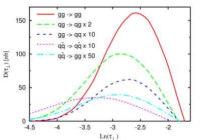
Figure 1: NLL resummed differential distribution $D(\tau_{\perp})\equiv d\Sigma(\tau_{\perp})/d\ln\tau_{\perp}$ for different underlying hard subprocesses.

The resulting distribution for $\tau_{\perp}$ is shown in fig. 1, decomposed into the most relevant underlying hard subprocesses, for the Tevatron run II regime ($\sqrt{s}=1.96$TeV). We select events containing two outgoing jets with $E_{\perp}>50$GeV and $|\eta|<1.0$ and use the CTEQ6M parton density set [17], corresponding to $\alpha_{s}(M_{Z})=0.118$. We have set $Q=\mu_{F}=\mu_{R}$ to be the Born partonic c.o.m. energy, though in future work we intend to explore a range of alternative scales. As is to be expected, channels with lower overall colour charge have broader distributions. We note that the different shapes of the various channels constitutes information that might be exploitable in fits of parton distributions. Of course detailed phenomenological analyses, both for perturbative and non-perturbative quantities, will also require matching to fixed-order predictions, another step that we leave to future work. Here we just remark that resummed results obtained from the master formula are in semi-analytical form (fully analytic but for the pure NLL function ${\cal{F}}$), so that they can be easily expanded to give the fixed-order coefficients needed when matching.

4 Conclusions

In this letter we have provided the elements needed for a novel, automated approach to general NLL resummation, specifically for the case of continuously global, exponentiable $(n\!+\!1)$-jet final-state observables in the $n$-jet limit. Results are obtained simply by specifying the Born process (and the number of hard partons) and providing the definition of the observable to be resummed in the form of a computer routine, similar to the long-established practice for fixed-order calculations, and in contrast to the tedious manual approach that has been used up to now for resummations. The results are provided in semi-analytical form, making it straightforward to obtain the expansions needed for procedures such as matching to fixed-order predictions.

We have demonstrated that the approach can be implemented in practice, by presenting automatically generated predictions for the transverse thrust in hadronic dijet production, the first event shape to be resummed in this important process. Only concerns for brevity prevent us from showing results for a range of other observables and processes, including several new observables in hadronic dijet production and jet rates in $e^{+}e^{-}$ and DIS.

An open question is whether such an approach, based on the analysis of classes of observables can be applied in other resummations contexts, or in the search for higher resummation accuracies. We enthusiastically advocate investigations in this direction.

Acknowledgments

We wish to thank Mrinal Dasgupta, Yuri Dokshitzer, Eric Laenen and Pino Marchesini for useful discussions and suggestions and Zoltan Nagy for providing us with the latest version of NLOJET++ and assistance in using it. We are grateful to each other’s institutes for hospitality and to CERN and the University of Milano-Bicocca for the use of computing facilities.

References

- [1] S. Bethke, J. Phys. G 26, R27 (2000).
- [2] S. Kluth et al., Eur. Phys. J. C 21, 199 (2001) and references therein.
- [3] V. A. Khoze and W. Ochs, Int. J. Mod. Phys. A 12, 2949 (1997) and references therein.
- [4] Yu. L. Dokshitzer, G. Marchesini and B. R. Webber, Nucl. Phys. B 469, 93 (1996); see also M. Beneke, Phys. Rept. 317, 1 (1999).
- [5] S. Catani, L. Trentadue, G. Turnock and B. R. Webber, Nucl. Phys. B 407, 3 (1993).
- [6] C. F. Berger, T. Kucs and G. Sterman, Phys. Rev. D 68, 014012 (2003)
- [7] N. Brown and W. J. Stirling, Phys. Lett. B 252, 657 (1990).
- [8] M. Dasgupta and G. P. Salam, Phys. Lett. B 512, 323 (2001); JHEP 0208, 032 (2002).
- [9] A. Banfi, G. P. Salam and G. Zanderighi, in preparation.
- [10] S. Catani, B. R. Webber and G. Marchesini, Nucl. Phys. B 349, 635 (1991); Yu. L. Dokshitzer, V. A. Khoze and S. I. Troyan, Phys. Rev. D 53, 89 (1996).
- [11] J. Botts and G. Sterman, Nucl. Phys. B 325, 62 (1989); N. Kidonakis, G. Oderda and G. Sterman, Nucl. Phys. B 531, 365 (1998).
- [12] A. Banfi, G. P. Salam and G. Zanderighi, JHEP 0201, 018 (2002).
- [13] A. Banfi, G. Marchesini, Yu. L. Dokshitzer and G. Zanderighi, JHEP 0007, 002 (2000); JHEP 0105, 040 (2001).
- [14] D. H. Bailey, “A Portable High Performance Multiprecision Package”, NASA Ames RNR Technical Report RNR-90-022; “A Fortran-90 Based Multiprecision System”, RNR Technical Report RNR-94-013.
- [15] I. A. Bertram [D0 Collaboration], Acta Phys. Polon. B 33, 3141 (2002).
- [16] Z. Nagy, Phys. Rev. Lett. 88, 122003 (2002); hep-ph/0307268.
- [17] J. Pumplin et al., JHEP 0207, 012 (2002).