On coherent radiation in electron-positron colliders

Abstract

The electromagnetic processes in linear colliders are discussed on the basis of quasiclassical operator method. The complete set of expressions is written down for spectral probability of radiation from an electron and pair creation by a photon taking into account both electron and photon polarization. Some new formulas are derived for radiation intensity and its asymptotics. The main mechanisms of pair creation dominate at $\chi\leq 1$ are discussed.

1 Introduction

The particle interaction at beam-beam collision in linear colliders occurs in an electromagnetic field provided by the beams. As a result, 1)the phenomena induced by this field turns out to be very essential, 2)the cross section of the main QED processes are modified comparing to the case of free particles. These items were considered by V.M.Strahkhovenko and authors [1], [2].

The magnetic bremsstrahlung mechanism dominates and its characteristics are determined by the value of the quantum parameter $\chi(t)$ dependent on the strength of the incoming beam field at the moment $t$ (the constant field limit)

$$\chi^{2}=-\frac{e^{2}}{m^{2}}(F_{\mu\nu}p_{\nu})^{2},\quad\chi=\frac{\gamma F}{H_{0}},$$ (1)

where $p^{\nu}(\varepsilon,\textbf{p})$ is a particle four-momentum, $F^{\mu\nu}$ is an external electromagnetic field tensor, $\gamma=\varepsilon/m$, $\textbf{F}=\textbf{E}_{\bot}+\textbf{v}\times\textbf{H}$, E and H are the electric and magnetic fields in the laboratory frame, $\textbf{E}_{\bot}=\textbf{E}-\textbf{v}(\textbf{vE})$, v is the particle velocity, $F=|\textbf{F}|$ and $H_{0}=m^{2}/e=(m^{2}c^{3}/e\hbar)=4.41\cdot 10^{13}$ Oe. We employ units $\hbar=c=1$ and $\alpha=1/137$,

1.1 General formulas

The photon radiation length in an external field is

$$l_{c}(\chi,u)=\lambda_{c}\frac{H_{0}}{F}\left(1+\frac{\chi}{u}\right)^{1/3}=\frac{\lambda_{c}\gamma}{\chi}\left(1+\frac{\chi}{u}\right)^{1/3},$$ (2)

where $\lambda_{c}=\hbar/mc$ is the electron Compton wave length, $u=\omega/\varepsilon^{\prime},\varepsilon^{\prime}=\varepsilon-\omega$, $\omega$ is the photon energy. The field of the incoming beam changes very slightly along the formation length $l_{c}$, if the condition $l_{c}\ll\sigma_{z}$ ($\sigma_{z}$ is the longitudinal beam size) is satisfied, providing a high accuracy of the magnetic bremsstrahlung approximation.

In the general case, when both polarizations of electron and photon are taken into account, the spectral probability of radiation from an electron per unit time has the form[3] (see also [2])

$$\frac{dw_{\gamma}}{dt}\equiv dW_{\gamma}(t)=\frac{\alpha}{2\sqrt{3}\pi\gamma^{2}}\Phi_{\gamma}^{\zeta}(1+(\mbox{\boldmath$\lambda$}\mbox{\boldmath$\xi$}))d\omega;~{}\Phi_{\gamma}^{\zeta}=\Phi_{\gamma}-\frac{\omega}{\varepsilon}(\mbox{\boldmath$\zeta$}{\bf h})K_{1/3}(z),$$

$$\Phi_{\gamma}(t)=\left(\frac{\varepsilon}{\varepsilon^{\prime}}+\frac{\varepsilon^{\prime}}{\varepsilon}\right)K_{2/3}(z)-\int_{z}^{\infty}K_{1/3}(y)dy,$$ (3)

where $K_{\nu}(z)$ is the Macdonald functions, $z=2u/3\chi(t)$, $\mbox{\boldmath$\lambda$}(\lambda_{1},\lambda_{2},\lambda_{3})$ are the Stokes parameters of emitted photons for the following choice of axes: ${\bf e}_{1}=({\bf v}\times{\bf h}),~{}{\bf h}={\bf F}^{\ast}/F,~{}{\bf e}_{2}={\bf h},~{}{\bf F}^{\ast}=e/|e|[{\bf H}_{\perp}+({\bf E}\times{\bf v})]$, $e$ is the charge of particle, $\zeta$ is the spin vector of the initial electron in its rest frame. The vector $\xi$ determines the mean photon polarization and its components are given by the following expressions:

$$\xi_{1}=\frac{\omega(\mbox{\boldmath$\zeta$}{\bf v}{\bf h})}{\varepsilon^{\prime}\Phi_{\gamma}^{\zeta}}K_{1/3}(z),\quad\xi_{3}=\frac{1}{\Phi_{\gamma}^{\zeta}}\left[K_{2/3}(z)+\frac{\omega}{\varepsilon^{\prime}}(\mbox{\boldmath$\zeta$}{\bf h})K_{1/3}(z)\right],$$

$$\xi_{2}=\frac{(\mbox{\boldmath$\zeta$}{\bf v})}{\Phi_{\gamma}^{\zeta}}\Bigg{[}\left(\frac{\varepsilon}{\varepsilon^{\prime}}-\frac{\varepsilon^{\prime}}{\varepsilon}\right)K_{2/3}(z)-\frac{\omega}{\varepsilon}\int_{z}^{\infty}K_{1/3}(y)dy\Bigg{]},$$ (4)

here $(\mbox{\boldmath$\zeta$}{\bf v}{\bf h})=\mbox{\boldmath$\zeta$}({\bf v}\times{\bf h})$.

Using asymptotic expansion of the Macdonald functions $K_{\nu}(z)=(\Gamma(\nu)/2)(2/z)^{\nu},~{}(z\ll 1)$ we obtain for the case $u\ll\chi$

$$\Phi_{\gamma}^{\zeta}=\Gamma\left(\frac{2}{3}\right)\left(\frac{3\chi}{u}\right)^{2/3}\left(1+\frac{\omega^{2}}{2\varepsilon\varepsilon^{\prime}}\right);$$

$$\xi_{1}=0,~{}\xi_{2}=\frac{\varepsilon^{2}-\varepsilon^{\prime 2}}{\varepsilon^{2}+\varepsilon^{\prime 2}}(\mbox{\boldmath$\zeta$}{\bf v}),~{}\xi_{3}=\frac{\varepsilon\varepsilon^{\prime}}{\varepsilon^{2}+\varepsilon^{\prime 2}}.$$ (5)

It is seen from given here characteristics that, generally speaking, the radiation is polarized. For unpolarized initial electrons $\xi_{3}\neq 0$.

The probability of pair creation by a photon in the external field can be find from formulas (3), (4) using the substitution rule [3]: $\varepsilon\rightarrow-\varepsilon,\quad\omega\rightarrow-\omega,\quad\mbox{\boldmath$\zeta$}\rightarrow-\mbox{\boldmath$\zeta$},\quad\lambda_{2}\rightarrow-\lambda_{2},\quad\lambda_{1,3}\rightarrow\lambda_{1,3}({\bf e}\rightarrow{\bf e}^{\ast}),\quad\omega^{2}d\omega\rightarrow-\varepsilon^{2}d\varepsilon$. Performing these substitutions we obtain

$$\frac{dw_{e}}{dt}\equiv dW_{e}(t)=\frac{\alpha m^{2}}{2\sqrt{3}\pi\omega^{2}}\Phi_{e}^{\zeta}(1+(\mbox{\boldmath$\lambda$}\mbox{\boldmath$\Sigma$}))d\varepsilon;~{}\Phi_{e}^{\zeta}=\Phi_{e}-\frac{\omega}{\varepsilon}(\mbox{\boldmath$\zeta$}{\bf h})K_{1/3}(y),$$

$$\Phi_{e}(t)=\left(\frac{\varepsilon}{\varepsilon^{\prime}}+\frac{\varepsilon^{\prime}}{\varepsilon}\right)K_{2/3}(y)+\int_{y}^{\infty}K_{1/3}(x)dx,,~{}\Sigma_{1}=-\frac{\omega(\mbox{\boldmath$\zeta$}{\bf v}{\bf h})}{\varepsilon^{\prime}\Phi_{e}^{\zeta}}K_{1/3}(y),$$

$$\Sigma_{2}=\frac{(\mbox{\boldmath$\zeta$}{\bf v})}{\Phi_{e}^{\zeta}}\Bigg{[}\left(\frac{\varepsilon}{\varepsilon^{\prime}}-\frac{\varepsilon^{\prime}}{\varepsilon}\right)K_{2/3}(y)+\frac{\omega}{\varepsilon}\int_{y}^{\infty}K_{1/3}(x)dx\Bigg{]},$$

$$\Sigma_{3}=-\frac{1}{\Phi_{e}^{\zeta}}\left[K_{2/3}(y)+\frac{\omega}{\varepsilon^{\prime}}(\mbox{\boldmath$\zeta$}{\bf h})K_{1/3}(y)\right],~{}y=\frac{2\omega^{2}}{3\varepsilon\varepsilon^{\prime}\kappa},~{}\kappa=\frac{\omega F}{mH_{0}}$$ (6)

here $\varepsilon$ is the energy of the created electron, $\varepsilon^{\prime}=\omega-\varepsilon$ is the energy of created positron, $\zeta$ is the electron spin vector, $\mbox{\boldmath$\lambda$}(\lambda_{1},\lambda_{2},\lambda_{3})$ are the Stokes parameters of the initial photon.

Integrating (6) over $\varepsilon$ (in some terms, integration by parts was carried out) we get the total probability of pair creation (per unit time) [4]

$$W_{e}^{\zeta}=\frac{1}{2}\left(W_{e}-\frac{\alpha m^{2}}{\sqrt{3}\pi\omega}(\mbox{\boldmath$\zeta$}{\bf h})\int_{0}^{1}\frac{K_{1/3}(\eta)}{x}dx\right),$$

$$W_{e}=\frac{2\alpha m^{2}}{3\sqrt{3}\pi\omega}\int_{0}^{1}K_{2/3}(\eta)\Bigg{[}\frac{1-3\lambda_{3}}{2}+\frac{1}{x(1-x)}\Bigg{]}dx,$$ (7)

where $x=\varepsilon/\omega$ and $\eta=2/(3\kappa x(1-x))$.

For longitudinally polarized initial electrons (see Eqs.(4),(5)) the hard photons ($\omega\simeq\varepsilon,~{}\varepsilon^{\prime}\ll\varepsilon$) are circularly polarized. The polarization of created electrons and positrons is discussed in detail in[5]. In particular, for the circular polarization of incoming photon the created electrons with $x\rightarrow 1$ have the longitudinal polarization (see (6)). All these effects are manifestation of ”the helicity transfer”.

2 Photon Emission

Here we consider radiation from unpolarized electrons. The spectral probability of radiation is (3)

$$\frac{dw_{\gamma}}{d\omega}=\frac{\alpha}{\pi\gamma^{2}\sqrt{3}}\int_{-\infty}^{\infty}\Phi_{\gamma}(t)dt.$$ (8)

For the Gaussian beams

$$\chi(t)=\chi_{0}(x,y)\exp(-2t^{2}/\sigma_{z}^{2}),$$ (9)

here the function $\chi_{0}(x,y)$ depends on transverse coordinates.

It turns out that for the Gaussian beams the integration of the spectral probability over time can be carried out in a general form:

$$\frac{dw_{\gamma}}{du}=\frac{\alpha m\sigma_{z}}{\pi\gamma\sqrt{6}}\frac{1}{(1+u)^{2}}\Bigg{[}\left(1+u+\frac{1}{1+u}\right)$$

$$\times\int_{1}^{\infty}K_{2/3}\left(ay\right)\frac{dy}{y\sqrt{\ln y}}-2a\int_{1}^{\infty}K_{1/3}\left(ay\right)\sqrt{\ln y}~{}dy\Bigg{]},$$ (10)

where $a=2u/3\chi_{0}$. In the case when $a\gg 1$ the main contribution into integral (10) gives the region $y=1+\xi,\xi\ll 1$. Taking the integrals over $\xi$ we obtain

$$\frac{dw_{\gamma}^{CF}}{du}\simeq\frac{\sqrt{3}\alpha m\sigma_{z}}{4\gamma}\frac{1+u+u^{2}}{u(1+u)^{3}}\chi_{0}\exp\left(-\frac{2u}{3\chi_{0}}\right)$$ (11)

For round beams the integration over transverse coordinates is performed with the density

$$n_{\perp}(\mbox{\boldmath$\varrho$})=\frac{1}{2\pi\sigma_{\perp}^{2}}\exp\left(-\frac{\varrho^{2}}{2\sigma_{\perp}^{2}}\right)$$ (12)

The parameter $\chi_{0}(\varrho)$ we present in the form

$$\chi_{0}(\varrho)=\chi_{m}\frac{f(x)}{f_{0}},\quad x=\frac{\varrho}{\sigma_{\perp}},\quad f(x)=\frac{1}{x}\left(1-\exp(-x^{2}/2)\right),$$

$$\chi_{rd}=0.720\alpha N\gamma\frac{\lambda_{c}^{2}}{\sigma_{z}\sigma_{\perp}},~{}f^{\prime}(x_{0})=0,~{}f_{0}=f(x_{0})=0.451256,$$ (13)

where $N$ is the number of electron in the bunch.

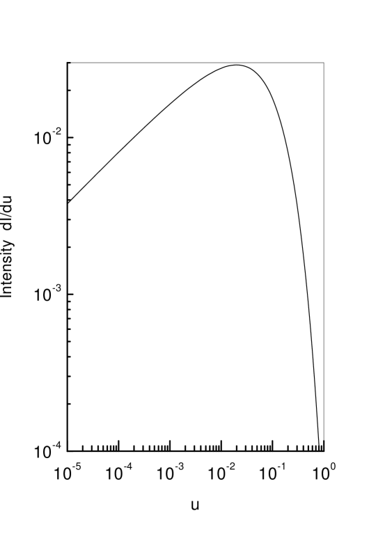
Figure 1: Spectral intensity of radiation of round beams in units $\alpha m^{2}\sigma_{z}$ for $\chi_{rd}$=0.13 calculated according to Eqs.(10),(13).

The Laplace integration of Eq.(11) gives for radiation intensity $dI/du=\varepsilon u/(1+u)dW/du$

$$\frac{dI_{as}}{du}\simeq\alpha m^{2}\sigma_{z}\frac{3}{4}\sqrt{\frac{\pi}{|f^{\prime\prime}_{0}|}}\frac{1+u+u^{2}}{\sqrt{u}(1+u)^{4}}f_{0}^{3/2}\chi_{rd}^{3/2}\exp\left(-\frac{2u}{3\chi_{rd}}\right),$$ (14)

where $f^{\prime\prime}_{0}=f^{\prime\prime}(x_{0})=-0.271678$.

Integration of (10) over transverse coordinates gives the final result for the radiation intensity. For the round beams it is shown in Fig.1 for $\chi_{rd}=0.13$, the curve attains the maximum at $u\simeq 0.02$. The right slope of the curve agrees with the asymptotic intensity (14) and the left slope of the curve agrees with the standard classical intensity.

$$\frac{dI_{cl}}{du}=\frac{e^{2}m^{2}}{\pi}3^{1/6}\Gamma(2/3)\chi^{2/3}u^{1/3}$$ (15)

It will be instructive to compare the spectrum in Fig.1, found by means of integration over the transverse coordinates with intensity spectrum which follows from Eq.(10) (multiplied by $\omega$) with averaged over the density Eq.(12) value $\chi_{0}$ Eq.(13): $\overline{\chi_{0}}=\chi_{rd}\cdot 0.8135$. The last spectrum reproduces the spectrum given in Fig.1, in the interval $10^{-3}\leq u/\overline{\chi_{0}}\leq 1$ with an accuracy better than 2% (near maximum better than 1%) while for $u/\overline{\chi_{0}}\leq 10^{-3}$ one can use the classic intensity (15) and for $u/\overline{\chi_{0}}\geq 1$ the asymptotics (14) is applicable.

For the flat beams ($\sigma_{x}\gg\sigma_{y}$) the parameter $\mbox{\boldmath$\chi$}_{0}(\mbox{\boldmath$\varrho$})$ takes the form

$$\mbox{\boldmath$\chi$}_{0}=\frac{2\gamma{\bf E}_{\perp}}{H_{0}}=\chi_{m}e^{-v^{2}}\left[\textbf{e}_{y}{\rm erf}\left(w\right)-i\textbf{e}_{x}{\rm erf}\left(iv\right)\right],\quad\chi_{m}=\frac{2N\alpha\gamma\lambda_{c}^{2}}{\sigma_{z}\sigma_{x}},$$ (16)

here $v=x/\sqrt{2}\sigma_{x},~{}w=y/\sqrt{2}\sigma_{y}$, ${\rm erf}(z)=2/\sqrt{\pi}\int_{0}^{z}\exp(-t^{2})dt$, $\textbf{e}_{x}$ and $\textbf{e}_{y}$ are the unit vectors along the corresponding axes. The formula (16) is consistent with given in [6]. In [1],[2] the term with $\textbf{e}_{x}$ was missed. Because of this the numerical coefficients in results for the flat beams are erroneous.

To calculate the asymptotics of radiation intensity for the case $u\gg\chi_{m}$ one has to substitute

$$\chi_{0}=|\mbox{\boldmath$\chi$}_{0}|=\chi_{m}e^{-v^{2}}\left[{\rm erf}^{2}\left(w\right)-{\rm erf}^{2}\left(iv\right)\right]^{1/2}$$ (17)

into Eq.(11) and take integrals over transverse coordinates $x,y$ with the weight

$$n_{\perp}(x,y)=\frac{1}{2\pi\sigma_{x}\sigma_{y}}\exp\left(-\frac{x^{2}}{2\sigma_{x}^{2}}-\frac{y^{2}}{2\sigma_{y}^{2}}\right).$$ (18)

Integral over $x$ can be taken using the Laplace method, while for integration over $y$ it is convenient to introduce the variable

$$\eta=\frac{2}{\sqrt{\pi}}\int_{w}^{\infty}\exp(-t^{2})dt,\quad w=\frac{y}{\sqrt{2}\sigma_{y}}.$$ (19)

As a result we obtain for the radiation intensity in the case of flat beams

$$\frac{dI_{fl}}{du}=\frac{9}{8\sqrt{2\left(1-2/\pi\right)}}\alpha m^{2}\sigma_{z}\chi_{m}^{5/2}\frac{1+u+u^{2}}{u^{3/2}(1+u)^{4}}\exp\left(-\frac{2u}{3\chi_{m}}\right).$$ (20)

It is interesting to compare the high-energy end of intensity spectrum at collision of flat beams (20) with intensity spectrum of incoherent radiation with regard for smallness of the transverse beam sizes [11]. For calculation we use the project TESLA parameters [8]:  $\varepsilon=250$ GeV, $\sigma_{x}=553$ nm, $\sigma_{y}=5$ nm, $\sigma_{z}=0.3$ mm, $N=2\cdot 10^{10}$, $\chi_{m}$=0.13. The result is shown in Fig.2, where the curves calculated according to Eq.(20), and Eq.(5.7) in [11]. It is seen that for $x=\omega/\varepsilon>0.7$ the incoherent radiation dominates. For $x>0.7$ the incoherent radiation may be used for a tuning of beams [11].

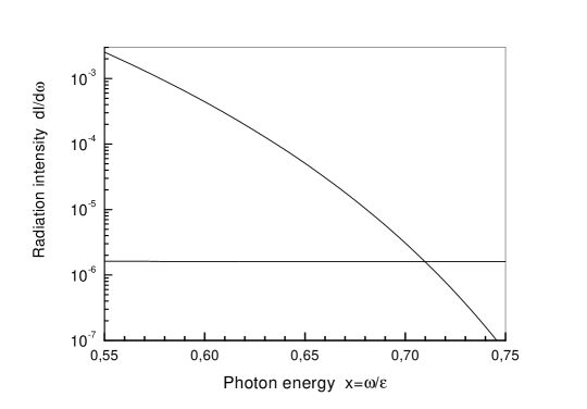
Figure 2: The spectral radiation intensity $dI/d\omega$ of coherent radiation (fast falling with $x=\omega/\varepsilon$ increase curve) and of incoherent radiation (the curve which is almost constant) in units $N\alpha^{2}\lambda_{c}/\sigma_{x}$ for beams with dimensions $\sigma_{x}=553$ nm, $\sigma_{y}=5$ nm, for $\chi_{m}$=0.13.

Along with the spectral characteristics of radiation the total number of emitted by an electron photons is of evident interest as well as the relative energy losses. We discuss an actual case of flat beams and the parameter $\chi_{m}\ll 1$. In this case one can use the classic expression for intensity (bearing in mind that at $\chi_{m}\geq 1/10$ the quantum effects become substantial). In classical limit the relative energy losses are

$$\frac{\Delta\varepsilon}{\varepsilon}=\frac{2\alpha m^{2}}{3\varepsilon}\int\chi^{2}(t,x,y)n_{\perp}(x,y)dtdxdy.$$ (21)

Using Eqs.(9), (17), and (18) we get

$$\frac{\Delta\varepsilon}{\varepsilon}=\frac{2}{9}\sqrt{\frac{\pi}{3}}r\chi_{m}^{2},\quad r=\frac{\alpha\sigma_{z}}{\gamma\lambda_{c}}.$$ (22)

For mean number of emitted by an electron photons we find

$$n_{\gamma}=\frac{5\alpha m^{2}}{2\sqrt{3}\varepsilon}\int\chi(t,x,y)n_{\perp}(x,y)dtdxdy=0.59275\frac{5}{2}\sqrt{\frac{\pi}{6}}r\chi_{m}=1.072r\chi_{m}.$$ (23)

If $\chi_{m}>1/10$ one have to use the quantum formulas. For the energy losses one can use the approximate expression (the accuracy is better than 2% for any $\chi$) [9]

$$d\varepsilon/dt=2/3\alpha m^{2}\chi^{2}\left[1+4.8(1+\chi)\ln(1+1.7\chi+2.44\chi^{2})\right]^{-2/3}.$$ (24)

Here $\chi$ is the local value, so this expression for $d\varepsilon/dt$ should be integrated over time and averaged over the transverse coordinates. For mean number of photons emitted by an electron there is the approximate expression (the accuracy is better than 1% for any $\chi_{0}$)[2]

$$n_{\gamma}(\mbox{\boldmath$\varrho$})=\frac{1.81\chi_{0}r}{[1+1.5(1+\chi_{0})\ln(1+3\chi_{0})+0.3\chi_{0}^{2}]^{1/6}},$$ (25)

where the expression should be averaged over the transverse coordinates. For the project TESLA one gets for $(\Delta\varepsilon/\varepsilon)_{cl}=4.3\%$ according to (22), while the correct result from (24) is $(\Delta\varepsilon/\varepsilon)_{cl}=3.2\%$. For mean number of emitted by an electron photons we have correspondingly $n_{\gamma}^{cl}\simeq 1.6$ while the correct result is $n_{\gamma}\simeq 1.5$.

3 Pair Creation

There are different mechanisms of electron-positron pair creation

1. Real photon radiation in the field and pair creation by this photon in the same field of the opposite beam. This mechanism dominates in the case $\chi\geq 1$.

2. Direct electroproduction of electro-positron pair in the field through virtual photon. This mechanism is also essential in the case $\chi\geq 1$.

3. Mixed mechanism(1):photon is radiated in the bremsstrahlung process, i.e. incoherently and the pair is produced in external field.

4. Mixed mechanism(2): photon is radiated in a magnetic bremsstrahlung way, and pair is produced in the interaction of this photon with individual particles of oncoming beam, i.e. in interaction with potential fluctuations.

5. Incoherent electroproduction of pair.

All these types of pair production processes were considered in detail in [2]. In the actual case $\chi\ll 1$ mixed and incoherent mechanisms mostly contribute. We start with the mixed mechanism (2). In the case $\chi_{m}\ll 1$ the parameter $\kappa$ Eq.(6) containing the energy of emitted photon is also small and the incoherent cross section of pair creation by a photon is weakly dependent on the photon energy

$$\sigma_{p}=28/9\alpha^{3}\lambda_{c}^{2}\ln(\sigma_{y}/\lambda_{c})\left(1+396\kappa^{2}/1225\right).$$ (26)

If the term $\propto\kappa^{2}$ being neglected, the pair creation probability is factorized (we discuss coaxial beams of identical configuration). The number of pairs created by this mechanism (per one initial electron) is

$$n_{p}^{(2)}=\int_{-\infty}^{\infty}W_{\gamma}(\mbox{\boldmath$\varrho$},t)dt\int_{t}^{\infty}2\sigma_{p}n_{\perp}(\mbox{\boldmath$\varrho$},t^{\prime})dt^{\prime}d^{2}\varrho$$

$$=\frac{35}{9}\sqrt{\frac{\pi}{6}}Nr\alpha^{3}\lambda_{c}^{2}\ln\frac{\sigma_{y}}{\lambda_{c}}\int\chi_{0}(\mbox{\boldmath$\varrho$})n_{\perp}^{2}(\mbox{\boldmath$\varrho$}d^{2}\varrho)=\frac{35}{9}\sqrt{\frac{\pi}{6}}Nr\chi_{m}\alpha^{3}\frac{\lambda_{c}^{2}}{2\pi\sigma_{x}\sigma_{y}}\frac{4}{\pi}$$

$$\times\int_{0}^{\infty}\exp(-3v^{2}-2w^{2})\big{[}{\rm erf}^{2}\left(w\right)-{\rm erf}^{2}\left(iv\right)\big{]}^{1/2}dwdv$$

$$=0.1167\alpha^{3}Nr\chi_{m}\frac{\lambda_{c}^{2}}{\sigma_{x}\sigma_{y}}\ln\frac{\sigma_{y}}{\lambda_{c}}.$$ (27)

So for the project TESLA parameters the total number of produced pairs by this mechanism per bunch in one collision is $Nn_{p}^{(2)}\sim 1.4\cdot 10^{4}$.

Now we turn over to discussion of incoherent electroproduction of pairs when both intermediate photons are virtual. To within the logarithmic accuracy for any $\chi$ and $\kappa$ one can use the method of equivalent photons

$$\frac{d\sigma_{v}}{d\omega}=n(\omega)\sigma_{p}(\omega),$$ (28)

where for soft photons $(\omega\ll\varepsilon)$

$$n(\omega)=\frac{2\alpha}{\pi}\ln\frac{\Delta}{q_{m}},~{}\Delta=m(1+\kappa)^{1/3},$$

$$q_{m}=m\frac{\omega}{\varepsilon}\left(1+\frac{\varepsilon\chi}{\omega}\right)^{1/3}+\frac{1}{\sigma_{y}}\equiv q_{F}+q_{\sigma}.$$ (29)

Taking into account that the cross section of pair photoproduction is

$$\sigma_{p}(\omega)=\frac{28\alpha^{3}}{9m^{2}}\ln\frac{m}{q_{m}(\omega^{\prime})},~{}\omega^{\prime}=\frac{m^{2}}{\omega}~{}(\kappa\ll 1);~{}\sigma_{p}\propto\kappa^{-2/3}~{}(\kappa\gg 1),$$ (30)

we obtain in the main logarithmic approximation for the cross section of the pair electroproduction

$$\sigma(2e\rightarrow 4e)=\frac{56\alpha^{4}}{9m^{2}}\int_{\omega_{min}}^{\omega_{max}}\ln\frac{m}{q_{m}(\omega)}\ln\frac{m}{q_{m}(\omega^{\prime})}\frac{d\omega}{\omega},$$ (31)

where $\omega_{max}=\varepsilon/(1+\chi),~{}\omega_{min}=m^{2}/\omega_{max}$. If we put $\chi=0,~{}\sigma_{y}=\infty$ we obtain the standard Landau-Lifshitz cross section $\sigma_{LL}$ (see e.g. [3])

$$\sigma_{LL}=\frac{28\alpha^{4}}{27m^{2}}\ln^{3}\gamma^{2}.$$ (32)

With regard for the bounded transverse dimensions of beam and influence of an external field the equivalent photon spectrum changes substantially. For $\chi\sim 1$ we have $q(\omega)=m(\omega/\varepsilon)^{2/3}+1/\sigma_{y}$ and under condition $\gamma^{2/3}\lambda_{c}/\sigma_{y}\geq 1$ we find

$$\sigma_{v}=\frac{28\alpha^{4}}{3m^{2}}\ln\left(\gamma^{4/3}\frac{\lambda_{c}}{\sigma_{y}}\right)\ln^{2}\frac{\sigma_{y}}{\lambda_{c}}.$$ (33)

For TESLA parameters $\gamma^{2/3}\lambda_{c}/\sigma_{y}\simeq 1$ then

$$\sigma_{v}=\frac{28\alpha^{4}}{81m^{2}}\ln^{3}\gamma^{2}.$$ (34)

This cross section is three times smaller than standard $\sigma_{LL}$. For the project TESLA parameters the number of pairs produced by this mechanism per bunch in one collision $n_{v}=L\sigma_{v}\simeq 1.5\cdot 10^{4},~{}L=1/(4\pi\sigma_{x}\sigma_{y})$ is the geometrical luminosity per bunch[11]. So the both discussed mechanisms give nearly the same contribution for this project.

It should be noted that the above analysis was performed under assumption that the configuration of beams doesn’t changed during collision, although in the TESLA project the disruption parameter $D_{y}>1$.

References

• [1] V.N.Baier, V.M.Katkov,and V.M.Strakhovenko, Particle Accelerators, 30, 43 (1990).
• [2] V.N.Baier, V.M.Katkov, and V.M.Strakhovenko, Preprint INP 89-180, Novosibirsk 1989 (unpublished).
• [3] V.N.Baier, V.M.Katkov,and V.S.Fadin, Radiation from Relativistic Electrons, Atomizdat, Moscow, 1973 (in Russian).
• [4] V.N.Baier, V.M.Katkov, and V.M.Strakhovenko, Phys. Lett. B229, 135 (1989).
• [5] V.N.Baier, V.M.Katkov, and V.M.Strakhovenko, Electromagnetic Processes at High Energies in Oriented Single Crystals, World Scientific, Singapore, 1998.
• [6] R.J.Noble, Nucl.Instr.Meth., A256, 427 (1987).
• [7] V.N.Baier, V.M.Katkov, and V.M.Strakhovenko, Sov.Phys.JETP, 67, 70 (1988).
• [8] O.Napoly, Proceedings of the 2001 Particle Accelerator Conference, Chicago, p.402, 2001.
• [9] V.N.Baier, V.M.Katkov, and V.M.Strakhovenko, Phys. Lett. A229, 429 (1992).
• [10] V.N.Baier, V.M.Katkov,and V.M.Strakhovenko, Sov.J.Nucl.Phys. 36, 95 (1982).
• [11] V.N.Baier, V.M.Katkov Phys. Rev, D66, 053009 (2002).